DualHSIC: HSIC-Bottleneck and Alignment for Continual Learning

Abstract

Rehearsal-based approaches are a mainstay of continual learning (CL). They mitigate the catastrophic forgetting problem by maintaining a small fixed-size buffer with a subset of data from past tasks. While most rehearsal-based approaches study how to effectively exploit the knowledge from the buffered past data, little attention is paid to the inter-task relationships with the critical task-specific and task-invariant knowledge. By appropriately leveraging inter-task relationships, we propose a novel CL method named DualHSIC to boost the performance of existing rehearsal-based methods in a simple yet effective way. DualHSIC consists of two complementary components that stem from the so-called Hilbert Schmidt independence criterion (HSIC): HSIC-Bottleneck for Rehearsal (HBR) lessens the inter-task interference and HSIC Alignment (HA) promotes task-invariant knowledge sharing. Extensive experiments show that DualHSIC can be seamlessly plugged into existing rehearsal-based methods for consistent performance improvements, and also outperforms recent state-of-the-art regularization-enhanced rehearsal methods. Source code will be released.

1 Introduction

Continual learning (CL) aims at enabling a single model to learn a sequence of tasks without catastrophic forgetting (McCloskey & Cohen, 1989) - the central problem of CL that models are prone to performance deterioration on previously seen tasks. A large body of work attempts to address CL from different perspectives (Kirkpatrick et al., 2017; Mallya & Lazebnik, 2018; Aljundi et al., 2018). Rehearsal-based methods (Aljundi et al., 2018; Chaudhry et al., 2019; Buzzega et al., 2020) have gained popularity due to their simplicity, effectiveness, and generality.

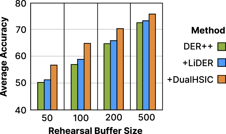
Figure 1: Comparison between DualHSIC, and two representative SOTA CL methods, LiDER and DER++. Both DualHSIC and LiDER are built upon DER++. DualHSIC achieves especially better performance with smaller buffer sizes.

The core idea of rehearsal is to maintain a small fix-sized memory buffer to save a subset of data from past tasks. When training on the current task, the model also revisits the buffered data to consolidate learned knowledge. Given the limited buffer size, it is challenging to keep generally discriminative representations for old tasks, because of overfitting (Verwimp et al., 2021). Existing methods mainly focus on data augmentation (Buzzega et al., 2020; Cha et al., 2021) and importance-based buffer example selection (Aljundi et al., 2019; Yoon et al., 2021).

Despite state-of-the-art (SOTA) performance, these approaches mostly consider how to better exploit knowledge from the buffered past data. It is notable that the inter-task relationship is also important yet under-investigated in rehearsal-based work: How does learning the current task affect the consolidation of past knowledge? To answer this question, we are inspired by the Complementary Learning Systems (CLS) (Kumaran et al., 2016; McClelland et al., 1995) theory and CLS-based CL methods (Pham et al., 2021; Wang et al., 2022b), which suggest that task-specific and task-invariant knowledge are critical for CL. Therefore, when learning the current task, we have to prevent the current task-specific knowledge from interfering with past knowledge, and leverage task-invariant knowledge to better consolidate the past.

A straightforward approach is to directly combine CLS-based methods with a rehearsal buffer. Although such an approach has proved effective, major components such as an additional backbone (Pham et al., 2021), prompting mechanisms (Wang et al., 2022b), or re-design of the rehearsal buffer system (Arani et al., 2022) are required. Ideally, one would prefer a more general method that can be seamlessly incorporated into most existing rehearsal-based methods with minimal tweaks.

To this end, we propose a novel CL method, DualHSIC, that improves existing rehearsal-based methods from a unique perspective: leveraging the so-called Hilbert-Schmidt independence criterion (HSIC) (Gretton et al., 2005) to learn better feature representations for rehearsal. HSIC is much more tractable and efficient than mutual information to measure statistical independence, and has been widely adopted for various sub-fields in machine learning (Wang et al., 2020b; Ma et al., 2020). DualHSIC consists of two complementary components: 1) HSIC-Bottleneck for Rehearsal (HBR) that mitigates inter-task interference by removing uninformative task-specific knowledge introduced by learning on the current task from the buffered data, such that inter-task interference and catastrophic forgetting are mitigated; 2) HSIC Alignment (HA) that encourages task-invariant knowledge sharing between current and past tasks for positive knowledge transfer (Hadsell et al., 2020). These components can be easily plugged into existing rehearsal-based methods with consistent performance improvement. In Figure 1, we demonstrate that DualHSIC outperforms advanced SOTA methods under different buffer sizes, with especially larger margins at small buffer sizes.

To further demonstrate the generality and effectiveness of DualHSIC, we also conduct comprehensive experiments on multiple CL benchmarks. We show that DualHSIC works collaboratively with various existing rehearsal-based CL methods, leading to consistent improvement upon SOTA results. We also conduct in-depth exploratory experiments to analyze the effectiveness of core designs of DualHSIC.

Overall, our work makes the following contributions:

• We propose DualHSIC, a general CL method that improves a wide spectrum of rehearsal-based methods. DualHSIC mitigates inter-task interference and encourages task-invariant knowledge sharing between tasks via the novel HBR and HA losses.

• Comprehensive experiments demonstrate that DualHSIC consistently improves SOTA rehearsal-based methods by at most $7.6\%$, and also outperforms stronger regularization-enhanced methods by at most $6.5\%$.

• To the best of our knowledge, our work is the first to bring HSIC to CL to learn better representations in a systematic way.

2 Related Work

Continual Learning. Existing CL works can be mainly categorized into regularization-based, architecture-based, and rehearsal-based approaches. Regularization-based approaches (Kirkpatrick et al., 2017; Zenke et al., 2017; Li & Hoiem, 2017; Aljundi et al., 2018) introduce additional terms in the loss function to penalize the model change on important weights for the purpose of protecting earlier tasks. Architecture-based approaches (Rusu et al., 2016; Mallya & Lazebnik, 2018; Wang et al., 2020a, 2022c; Yan et al., 2021) dynamically expand the model capacity or isolate existing model weights to reduce the interference between the new tasks and the old ones. Rehearsal-based approaches allow access to a memory buffer with examples from prior tasks and train the model jointly with the current task. With its simplicity and efficacy, the idea of rehearsal enjoys great popularity and has been adopted by many state-of-the-art methods (Buzzega et al., 2020; Cha et al., 2021; Pham et al., 2021; Wang et al., 2022a). In this work, we present DualHSIC as a general surrogate loss that improves rehearsal-based methods.

Hilbert Schmidt Independence Criterion (HSIC). As a statistical dependency measure, HSIC (Gretton et al., 2005) has been widely applied in various machine learning applications, such as dimensionality reduction (Niu et al., 2011), clustering (Wu et al., 2020), feature selection (Song et al., 2012), and class discovery (Wang et al., 2020b). HSIC captures non-linear dependencies between random variables and has the advantage of easy empirical estimation over mutual information (MI). Recently, Ma et al. (2020) propose the HSIC-bottleneck as an alternative for cross-entropy loss. Wang et al. (2021) and Jian et al. (2022) further demonstrate how HSIC-bottleneck strengthens a model’s adversarial robustness. However, no prior work has studied the application of HSIC under the context of CL. As a very first attempt, we propose two novel complementary HSIC-related losses that address catastrophic forgetting from a unique perspective.

Among the latest CL works, OCM (Guo et al., 2022) and LiDER (Bonicelli et al., 2022) are the closest to our work, in terms of the common target to improve rehearsal-based methods via surrogate loss terms. However, we would still like to emphasize that our work is different and novel. OCM proposes an MI-based loss through a complicated contrastive learning proxy (Oord et al., 2018), while our work introduces two different HSIC losses with a simple empirical evaluation strategy. LiDER constrains the Lipschitz constant of a model to strengthen the robustness of the decision boundary, while DualHSIC has a totally different motivation and methodology. Moreover, different from both works, we explicitly consider the inter-task relationship in CL. We also show that DualHSIC outperforms OCM and LiDER consistently in practice (Table 2).

3 Preliminaries

3.1 Continual Learning Problem Setting

In supervised continual learning, a sequence of tasks $\mathcal{D}=\{\mathcal{D}_{1},\ldots,\mathcal{D}_{T}\}$ arrive in a streaming fashion, where each task $\mathcal{D}_{t}=\{({\bm{x}}^{t}_{i},y^{t}_{i})\}_{i=1}^{n_{t}}$ contains a separate target dataset, i.e., $\mathcal{D}_{i}\cap\mathcal{D}_{j}=\emptyset$. A single model needs to adapt to them sequentially, with only access to $\mathcal{D}_{t}$ at the $t$-th task. In practice, we allow a small fix-sized rehearsal buffer $\mathcal{M}$ to save data from past tasks. At test time, we mainly focus on one of the most challenging class-incremental (Class-IL) setting, where no task identity is available for the coming test examples.

In general, given a prediction model $h_{\theta}$ parameterized by $\theta$, a large body of continual learning work seeks to optimize for the following loss at the $t$-th task:

$$\small\begin{split}\mathcal{L}_{\text{CL}}(\theta)=\sum_{{\bm{x}},y\in\mathcal{D}_{t}}\ell(h_{\theta}({\bm{x}}),y)+\sum_{{\bm{x}}^{M},y^{M}\in\mathcal{M}}\ell_{\mathcal{M}}(h_{\theta}({\bm{x}}^{M}),y^{M}),\end{split}$$ (1)

where $\ell$ and $\ell_{\mathcal{M}}$ are losses for the current data and buffered data, respectively. For example, Chaudhry et al. (2019) applies cross-entropy as both losses, while many recent works present different losses or add additional auxiliary loss terms (Buzzega et al., 2020; Cha et al., 2021). Although $\mathcal{L}_{\text{CL}}$ can take many forms depending on the actual method, our method DualHSIC presents a model-agnostic loss that can be plugged into most rehearsal-based CL methods to improve the overall performance.

3.2 Hilbert-Schmidt Independence Criterion

The Hilbert-Schmidt independence criterion (HSIC) is a statistical measure for identifying dependencies between two random variables, which was first introduced by Gretton et al. (2005). HSIC calculates the Hilbert-Schmidt norm of the cross-covariance operator of the distributions in the Reproducing Kernel Hilbert Space (RKHS). Similar to the widely used Mutual Information (Shannon, 1948), HSIC is able to detect non-linear dependencies with the advantage of easy empirical estimation over MI.

Given two random variables $X$ and $Y$, the HSIC between them is formally defined as:

$$\begin{split}\operatorname{HSIC}&(X,Y)=\mathbb{E}_{XYX^{\prime}Y^{\prime}}\left[k_{X}\left(X,X^{\prime}\right)k_{Y^{\prime}}\left(Y,Y^{\prime}\right)\right]\\ &+\mathbb{E}_{XX^{\prime}}\left[k_{X}\left(X,X^{\prime}\right)\right]\mathbb{E}_{YY^{\prime}}\left[k_{Y}\left(Y,Y^{\prime}\right)\right]\\ &-2\mathbb{E}_{XY}\left[\mathbb{E}_{X^{\prime}}\left[k_{X}\left(X,X^{\prime}\right)\right]\mathbb{E}_{Y^{\prime}}\left[k_{Y}\left(Y,Y^{\prime}\right)\right]\right],\end{split}$$ (2)

where $X^{\prime}$, $Y^{\prime}$ are independent copies of $X$, $Y$, respectively, and $k_{X}$, $k_{Y}$ are corresponding kernel functions.

HSIC can be easily approximated empirically without knowing the analytical form of distribution $P_{XY}$. Given $n$ i.i.d. examples $\{({\bm{x}}_{i},y_{i})\}_{i=1}^{n}$ sampled from $P_{XY}$, the empirical estimation of HSIC is:

$${\operatorname{HSIC}}_{e}(X,Y)={(n-1)^{-2}}\operatorname{tr}\left(K_{X}HK_{Y}H\right),$$ (3)

where $K_{X}$ and $K_{Y}$ are kernel matrices with $K_{X_{ij}}=k_{X}({\bm{x}}_{i},{\bm{x}}_{j})$ and $K_{Y_{ij}}=k_{Y}(y_{i},y_{j})$, respectively, $\operatorname{tr}(\cdot)$ is the trace operator, and $H=\mathbf{I}-\frac{1}{n}\mathbf{1}\mathbf{1}^{\top}$ is a centering matrix. In our experiments, we evaluate HSIC terms via this empirical estimation.

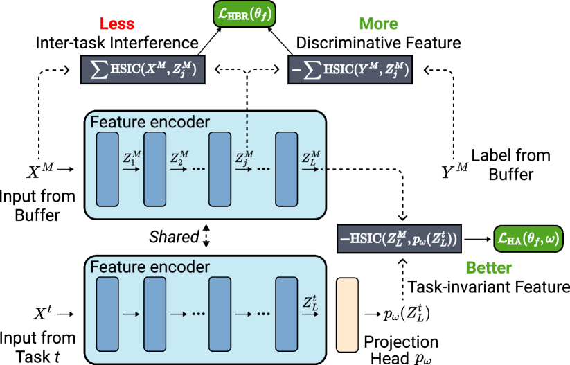
Figure 2: Overview of DualHSIC. HBR is calculated on the buffered data in a multi-layer fashion. However, only a sub-component of HBR at the $j$-th intermediate layer is illustrated in the figure for visual clarity. HA is calculated between the latent representations of buffered and current data. Both inputs share the same feature encoder and an MLP projection head is used to create an alternative view. Note that the actual HA is symmetric, exchanging two input branches in the figure provides the second half of the loss.

4 DualHSIC

In this section, we will present DualHSIC, a general continual learning objective that is orthogonal to the existing rehearsal-based framework. As shown in Figure 2, DualHSIC consists of two complementary losses: HSIC-Bottleneck for Rehearsal, which mitigates inter-task interference, and HSIC Alignment which encourages the sharing of task-invariant knowledge between tasks.

4.1 HSIC Bottleneck for Rehearsal

During the continual learning process, compared with abundant data from the current task, we only have very limited buffered data from past tasks. This data-imbalance (Hadsell et al., 2020; Mai et al., 2021) issue makes the model over-focus on task-specific knowledge of the current task, leading to performance deterioration on the past tasks. To address the problem, we propose HSIC-Bottleneck for Rehearsal (HBR), a general loss to mitigate inter-task interference and retrain good feature representations for data saved in the rehearsal buffer.

We denote the model, a multi-layer feedforward neural network with $L$ intermediate layers, used in the CL process by $h_{\theta}:\mathbb{R}^{d_{x}}\to\mathbb{R}^{C}$, where $d_{x}$ is the input dimension and $C$ is the total number of classes of interest during CL. We also decompose $h_{\theta}=g_{\theta_{g}}\circ f_{\theta_{f}}$ into the final classification layer $g_{\theta_{g}}$ and the feature encoder $f_{\theta_{f}}$ for notation convenience. We use $X^{M}$ to denote the random variable that represents data saved in the rehearsal buffer $\mathcal{M}$, we further denote by $Z^{M}_{j}\in\mathbb{R}^{d_{z_{j}}}$ its corresponding output of the $j$-th intermediate layer. HSIC-Bottleneck for Rehearsal (HBR) is defined as a penalty loss on the buffered data:

where $\lambda_{x}$ and $\lambda_{y}$ are balancing coefficients.

Mitigating Inter-Task Interference. Intuitively, minimizing the HSIC between $X^{M}$ and $Z^{M}_{j}$ aims at reducing the noisy information contained within the latent representation $Z^{M}_{j}$ w.r.t. the input $X^{M}$. When learning the current task $t$, the model undoubtedly extracts useful knowledge from the current data. However, such task-specific knowledge may be uninformative or noisy for past tasks (Ebrahimi et al., 2020; Pham et al., 2021; Wang et al., 2022b). Therefore, by only applying the bottleneck loss to the buffered data, we implicitly mitigate the interference from learning task-specific knowledge for the current task to past tasks.

Maintaining Discriminative Knowledge. HBR also tries to maximize the HSIC between $Y^{M}$ and $Z^{M}_{j}$, which naturally retains the discriminative information useful for classification. Although it serves a similar purpose as the cross-entropy loss for classification, Wang et al. (2021) demonstrate the necessity of this term in the bottleneck loss empirically; we also verify this observation in our ablation study (Section 5.4).

Asynchronous Consolidation. Note that we only apply HBR to the buffered data, instead of both buffered and current data. Empirically, we observe that adding the term to both data does not lead to performance improvement (Appendix C.5); similar results have also been observed by Bonicelli et al. (2022). Intuitively, we already have abundant data for the current task compared to the buffered data, so the learning of the current task is much less prone to inter-task interference. On the other hand, our proposed scheme naturally consolidates knowledge in an asynchronous way to address the stability-plasticity dilemma for continual learners (Abraham & Robins, 2005; Mermillod et al., 2013): the model first learns the current task without HBR for maximum plasticity, then rehearse the learned task in future tasks with HBR to maintain stability.

Alternative Perspective via Robustness. Although not used in the context of CL, HSIC-bottleneck has been proved by Wang et al. (2021) both empirically and theoretically to improve the adversarial robustness of the model. Interestingly,  Bonicelli et al. (2022) also demonstrate that a more adversarially robust model on the buffered data prevents the decision boundary from eroding, thus mitigating catastrophic forgetting. In this respect, HBR provides another bridge that links adversarial robustness with catastrophic forgetting.

Input: Model $h_{\theta}$ with $L$-layer feature encoder $f_{\theta_{f}}$ and classifier $g_{\theta_{g}}$, projection head $p_{\omega}$, number of tasks $T$, training epochs of the $t$-th task $K_{t}$, mini-batch size $B$.

Initialize: $\theta$ ($\theta_{f}$ and $\theta_{g}$), $p_{\omega}$

for $t=1,\ldots,T$ do

       for $e=1,\ldots,K_{t}$ do

             Draw a mini-batch $\{({\bm{x}}^{t}_{i},y^{t}_{i})\}_{i=1}^{B}$ from current task

             Draw a mini-batch $\{({\bm{x}}^{M}_{i},y^{M}_{i})\}_{i=1}^{B}$ from buffer

             Generate latent representations for buffered data at every intermediate layer $\{\{z^{M}_{i,j}\}_{i=1}^{B}\}_{j=1}^{L}$

             Generate latent representation for current data at the last intermediate layer $\{z^{t}_{i,L}\}_{i=1}^{B}$

            /* HSIC Bottleneck for Rehearsal */

             Compute $\mathcal{L}_{\text{HBR}}(\theta_{f})$ in Eq. (4) via mini-batched empirical estimation (Eq. (3), same below)

            /* HSIC Alignment */

             Generate projected views of the last layer representations $\{p_{\omega}(z^{t}_{i,L})\}_{i=1}^{L}$ and $\{p_{\omega}(z^{M}_{i,L})\}_{i=1}^{L}$

            Compute $\mathcal{L}_{\text{HA}}(\theta_{f},\omega)$ in Eq. (5)

            /* Original Rehearsal Loss */

             Compute $\mathcal{L}_{\text{CL}}(\theta)$ from the base rehearsal method

            Compute $\mathcal{L}_{\text{total}}$ in Eq. (6).

            Update $\theta=\{\theta_{f},\theta_{g}\}$ and $\omega$ via back-propagation

       end for

      

end for

Algorithm 1 DualHSIC for Continual Learning

4.2 HSIC Alignment Loss

According to the complementary learning systems (CLS) theory (McClelland et al., 1995; Kumaran et al., 2016), learning task-invariant knowledge that can be shared between tasks is also critical in CL. To this end, we propose a novel HSIC Alignment (HA) loss to better capture task-invariant knowledge.

Recall that we denote by $X^{M}$ the random variable for the buffered data, and $Z^{M}_{L}$ the latent representation from the last intermediate layer. We further denote by $X^{t}$ the random variable for the data from the current task $t$, as well as the corresponding latent representation $Z^{t}_{L}$. We define the HSIC Alignment (HA) loss as:

where $p_{\omega}$ is an multi-layer perceptron (MLP) projection head (Grill et al., 2020; Chen & He, 2021) for producing multiple views of the latent representation.

Strengthening Task-Invariant Knowledge. HA aims at maximizing the HSIC between the latent representations of examples from different tasks such that task-invariant knowledge can be better shared. Note that HA actually acts as a complementary learning objective to HBR, as it encourages knowledge transfer between tasks in addition to less forgetting (Hadsell et al., 2020).

Design Choices. The design of the HA loss is inspired by the Siamese representation learning paradigm (Chen & He, 2021). In practice, we have empirically verified the effectiveness of the symmetrized loss and the necessity of adding the projection head. Interestingly, HA works quite well without the stop-gradient (Chen & He, 2021) operation. We suspect that this phenomenon may due to the fact that the intrinsic difference between examples from different tasks ensures latent representations do not collapse. We leave further theoretical explorations in our future work.

Table 1: Performance (in average accuracy) comparison between DualHSIC with state-of-the-art rehearsal-based methods on benchmark datasets with different buffer sizes and optional pre-training. All results are averaged through three independent runs.

Method	Split CIFAR-10			Split CIFAR-100						Split miniImageNet
Pre-training	✗			✗			Tiny ImageNet			✗
Upper bound	92.38			73.29			75.20			53.55
Sequential	19.67			9.29			9.52			4.51
Buffer size	$100$	$200$	$500$	$200$	$500$	$2000$	$200$	$500$	$2000$	$1000$	$2000$	$5000$
ER	36.39	44.79	57.74	14.35	19.66	36.76	18.09	28.25	43.18	8.37	16.49	24.17
+ DualHSIC	43.70	49.37	61.65	21.57	26.65	40.26	25.35	33.82	46.57	12.71	19.57	26.89
X-DER-RPC	59.29	65.19	68.10	35.34	44.62	54.44	51.40	57.45	62.46	25.24	26.38	29.91
+ DualHSIC	66.76	71.05	73.53	40.04	46.83	54.71	52.67	57.88	62.70	27.21	28.15	31.09
ER-ACE	53.90	63.41	70.53	26.28	36.48	48.41	41.85	48.19	57.34	17.95	22.60	27.92
+ DualHSIC	60.52	68.08	73.78	29.08	38.94	50.55	45.19	50.36	57.50	22.33	25.41	30.12
DER++	57.65	64.88	72.70	25.11	37.13	52.08	26.50	43.65	58.05	18.02	23.44	30.43
+ DualHSIC	64.98	70.28	75.94	31.46	41.86	53.53	34.10	50.64	59.02	24.78	29.37	34.98

4.3 Overall Objective

At every task, we incorporate both the HBR and HA losses into the existing rehearsal-based learning framework. Therefore, the overall objective is:

$$\begin{split}\mathcal{L}_{\text{total}}&=\mathcal{L}_{\text{CL}}(\theta)+\mathcal{L}_{\text{HBR}}(\theta_{f})+\lambda_{\text{HA}}\mathcal{L}_{\text{HA}}(\theta_{f},\omega),\\ &=\sum_{{\bm{x}},y\in\mathcal{D}_{t}}\ell(h_{\theta}({\bm{x}}),y)+\sum_{{\bm{x}}^{M},y^{M}\in\mathcal{M}}\ell_{\mathcal{M}}(h_{\theta}({\bm{x}}^{M}),y^{M})+\\ &\quad\underbrace{\lambda_{x}\sum_{j=1}^{L}\operatorname{HSIC}(X^{M},Z^{M}_{j})-\lambda_{y}\sum_{j=1}^{L}\operatorname{HSIC}(Y^{M},Z^{M}_{j})}_{\textrm{HSIC-Bottleneck for Rehearsal}}-\\ &\quad\lambda_{\text{HA}}\underbrace{\frac{1}{2}\left(\operatorname{HSIC}(Z^{M}_{L},p_{\omega}(Z^{t}_{L}))+\operatorname{HSIC}(p_{\omega}(Z^{M}_{L}),Z^{t}_{L})\right)}_{\textrm{HSIC Alignment}},\end{split}$$ (6)

where $\lambda_{\text{HA}}$ is a balancing coefficient. Note that our surrogate loss terms are general enough to be combined with and further improve almost any existing rehearsal methods. The overall algorithm is described in Alg. 1. In practice, we evaluate HSIC empirically via (3) in mini-batches, following (Wang et al., 2021). Given mini-batch size $B$, the maximum intermediate dimension $d_{Z}=\max_{j}d_{Z_{j}}$, the computation complexity of evaluating the emiprical HSIC is $\mathcal{O}(B^{2}d_{Z})$ (Song et al., 2012). Thus, the computational complexity overhead introduced by DualHSIC is $\mathcal{O}(LB^{2}d_{Z})$.

5 Experiments

To evaluate the efficacy of the proposed DualHSIC, we conduct comprehensive experiments on representative CL benchmarks, closely following the challenging class-incremental learning setting in prior works (Lopez-Paz & Ranzato, 2017; Van de Ven & Tolias, 2019; Wang et al., 2022c). We incorporate DualHSIC with multiple SOTA rehearsal-based CL methods to demonstrate performance improvement, while also comparing DualHSIC against other SOTA CL methods. We also performed an ablation study and exploratory experiments to further showcase the effectiveness of individual components.

Table 2: Performance (in average accuracy) comparison between DualHSIC and regularization-enhanced rehearsal methods on various benchmark datasets. ER-ACE and DER++ are representative rehearsal-based methods that all comparing methods build upon. All results are averaged through three independent runs.

Method	Split CIFAR-10			Split CIFAR-100			Split miniImageNet
Buffer size	$100$	$200$	$500$	$200$	$500$	$2000$	$1000$	$2000$	$5000$
ER-ACE	53.90	63.41	70.53	26.28	36.48	48.41	17.95	22.60	27.92
+ sSGD	56.26	64.73	71.45	28.07	39.59	49.70	18.11	22.43	24.12
+ oEwC	52.36	61.09	68.70	24.93	35.06	45.59	19.04	24.32	29.46
+ oLAP	52.76	63.19	70.32	26.42	36.58	47.66	18.34	23.19	28.77
+ OCM	57.18	64.65	70.86	28.18	37.74	49.03	20.32	24.32	28.57
+ LiDER	56.08	65.32	71.75	27.94	38.43	50.32	19.69	24.13	30.00
+ DualHSIC	60.52	68.08	73.78	29.08	38.94	50.55	22.33	25.41	30.12
DER++	57.65	64.88	72.70	25.11	37.13	52.08	18.02	23.44	30.43
+ sSGD	55.81	64.44	72.05	24.76	38.48	50.74	16.31	19.29	24.24
+ oEwC	55.78	63.02	71.64	24.51	35.22	51.53	18.87	24.53	31.91
+ oLAP	54.86	62.54	71.38	23.26	34.48	50.80	18.91	25.02	32.78
+ OCM	59.25	65.81	73.53	27.46	38.94	52.25	20.93	24.75	31.16
+ LiDER	58.43	66.02	73.39	27.32	39.25	53.27	21.58	28.33	35.04
+ DualHSIC	64.98	70.28	75.94	31.46	41.86	53.53	24.78	29.37	34.98

5.1 Experiment Setting

Evaluation Benchmarks. We evaluate our DualHSIC on three representative CL benchmarks, following mainstream evaluation paradigms (Zenke et al., 2017; Buzzega et al., 2020; Bonicelli et al., 2022).
- Split CIFAR-10 originates from the well-known CIFAR-10 (Krizhevsky et al., 2009) dataset. It is split into 5 disjoint tasks with 2 classes per task.
- Split CIFAR-100 is also a split version of CIFAR-100 (Krizhevsky et al., 2009), which contains 10 disjoint tasks with 10 classes per task.
- Split miniImageNet is subsampled from ImageNet (Deng et al., 2009) with $100$ classes. It is split into 20 disjoint tasks with 5 classes per task. Dataset licensing information can be found in Appendix A.

Comparing Methods. We compare DualHSIC of multiple SOTA CL methods of different kinds.
- Rehearsal-Based. DualHSIC is a general framework that can be combined with almost any mainstream rehearsal-based methods. Therefore, we incorporate DualHSIC into multiple SOTA rehearsal-based methods, including ER (Chaudhry et al., 2019), DER++ (Buzzega et al., 2020), X-DER-RPC (Boschini et al., 2022), and ER-ACE (Caccia et al., 2021), to demonstrate its general effectiveness.
- Regularization-Based. Note that DualHSIC can also be regarded as a novel regularizer in addition to the original rehearsal-based loss. Therefore, We also compare our method with existing regularization-based techniques based on ER-ACE and DER++, including sSGD (Mirzadeh et al., 2020), oEWC (Schwarz et al., 2018), oLAP (Ritter et al., 2018), and more recent SOTA methods, OCM (Guo et al., 2022) and LiDER (Bonicelli et al., 2022).
- Reference Baselines. For completeness, we also include the naive baseline, Sequential, that trains a model sequentially on tasks without any buffer, and the possible Upper bound, that trains the model on the union of all tasks in an i.i.d. fashion, for reference.

Evaluation Metrics. We report two major metrics that are widely used in previous works (Chaudhry et al., 2018; Lopez-Paz & Ranzato, 2017; Mai et al., 2021): Average accuracy (higher is better) and Forgetting (lower is better) is used to evaluate the performance of the final model trained sequentially on all tasks. The formal definition of both metrics are shown in Appendix B. Note that we include average accuracy as our main result, while keep the forgetting results and error bars in Appendix C.3 and C.2 due to space limit.

Experimental Details. We follow the standard settings in prior CL work (Buzzega et al., 2020; Bonicelli et al., 2022) for a fair comparison. For hyperparameters of the base rehearsal methods, we refer (Buzzega et al., 2020) for the best configurations. All methods use the same backbone model, training epochs and batch sizes for fair comparison. The per-task training epochs are set as 50 for Split CIFAR-10/100, and 80 for Split miniImageNet. The batch sizes are set as 32, 64, and 128 for Split CIFAR-10, Split CIFAR-100, and Split miniImageNet, respectively. We adopt ResNet-18 (He et al., 2016) without any pre-training for Split CIFAR-10 and Split CIFAR-100. Additionally, we experiment on Split CIFAR-100 using ResNet-18 pre-trained on Tiny ImageNet as reported in (Bonicelli et al., 2022). For Split miniImageNet, EfficientNet-B2 (Tan & Le, 2019) without pre-training is used. For the projection head, we use a $128$-$512$-$128$ MLP and a $352$-$1408$-$352$ MLP for ResNet-18 and EfficientNet-B2, respectively. To implement the empirical HSIC, we adopt the commonly used Gaussian kernel with $\sigma=5$, following the recommendations by Wang et al. (2021). Additional details about the selection of balancing coefficients are reported in Appendix C.1.

For the comparing methods, we either directly take existing results reported in Bonicelli et al. (2022), or reproduce the experiment results using the suggested hyperparameters from their original papers.

Computing Resources. All experiments are conducted on a single Tesla V100 GPU with 32GB memory.

5.2 Comparison with Rehearsal Methods

Table 1 presents our evaluation results comparing DualHSIC with multiple SOTA rehearsal-based models. We can see that DualHSIC can consistently improve the performance of all base methods in almost all evaluated scenarios, in terms of both average accuracy and forgetting (Appendix C.3). In particular, the maximum performance gain of DualHISC is $7.6\%$ across all datasets and buffer sizes. Interestingly, we observe the largest performance gap when buffer size is small in Table 1, while similar trend is revealed in Figure 1 as well. This observation actually confirms the effectiveness of DualHSIC under more challenging scenarios. As suggested by Prabhu et al. (2020), when buffer size is large, the data imbalance issue between buffered and current data is naturally mitigated. Moreover, we observe that the effectiveness of DualHSIC is orthogonal to pre-trainig, showing the potential that DualHSIC can be useful in real-world scenarios that often involves learning from a pre-trained model (Wang et al., 2022c).

5.3 Comparison with Regularization-Enhanced Rehearsal Methods

To further demonstrate the effectiveness of DualHSIC, we compare DualHSIC against regularization-enhanced rehearsal methods by combining existing regularization techniques and replay strategies including ER-ACE and DER++. We show the experiment results in Table 2. DualHSIC outperforms almost all regularization techniques on all benchmarks with various buffer sizes, by at most $6.5\%$ margin. Even when DualHSIC is outperformed, its gap with the top performer is minimal ($<0.6\%$). Similarly, we observe the clear advantage of DualHSIC at the small buffer regime. Note that sSGD, oEwC and oLAP do not specifically consider buffered data, while OCM and LiDER do not explicitly consider the inter-task relationship as DualHSIC does, which may account for the larger performance gap when buffer size is small.

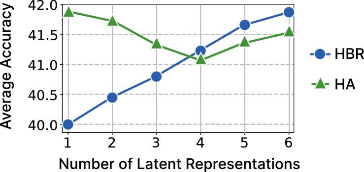
Figure 3: Effectiveness of HBR and HA w.r.t. number of latent representations included. HBR gets increasingly better performance with more latent representations, while HA gets the best performance with a single latent representation.

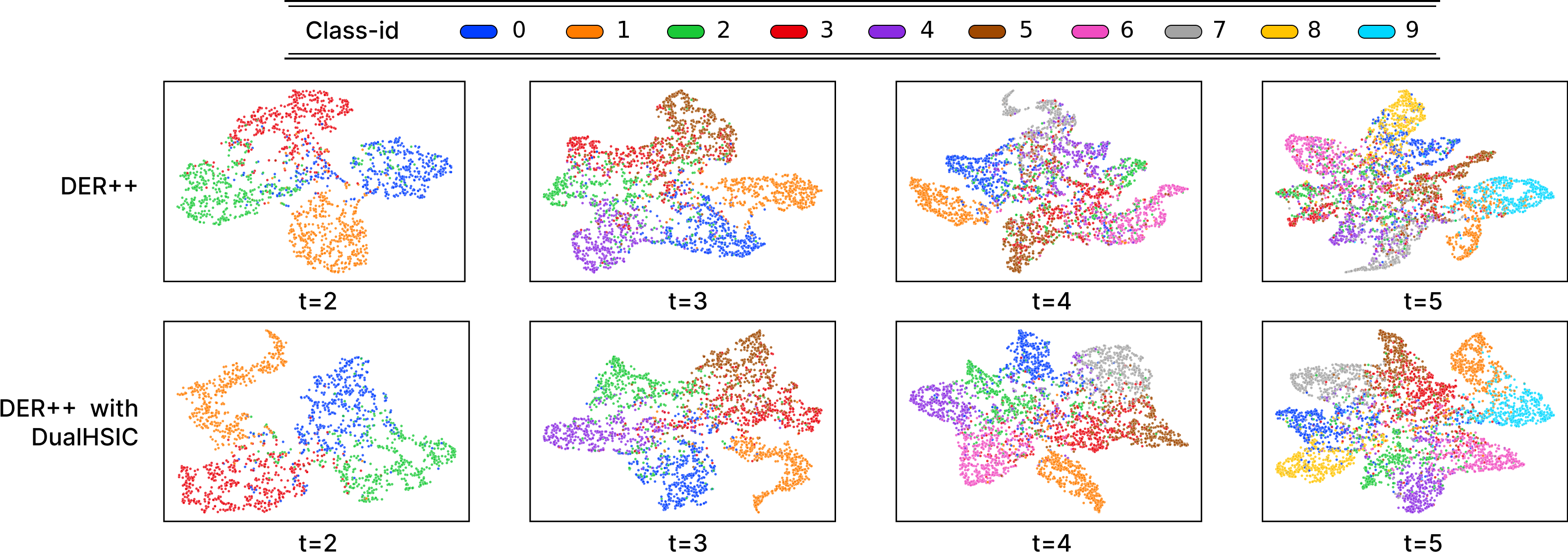
Figure 4: Comparison of tSNE visualization of the last latent representation between DER++ vs. DER++ with DualHSIC. We show the progress of tSNE embeddings starting from task $2$, since task $1$ can be regarded as trivial supervised learning with no catastrophic forgetting issue. Classes are split into 5 tasks based on their label ID, i.e., 2 consecutive classes are assigned to the same task. DualHSIC improves DER++ with more separable embeddings and less inter-class confusion at later tasks.

Table 3: Ablation study on Split CIFAR-100 with 500 buffer size, $\mathcal{L}_{\text{CL}}$ is based on DER++. $\operatorname{H}(\cdot;\cdot)$ represents $\operatorname{HSIC}(\cdot;\cdot)$. “Proj.” and “Sym.” are abbreviations for using projection head $p_{\omega}$ and using symmetric loss, respectively.

$\mathcal{L}_{\text{CL}}$	$\mathcal{L}_{\text{HBR}}$		$\mathcal{L}_{\text{HA}}$		Class-IL Acc ($\uparrow$)
	$\operatorname{H}(X;Z)$	$\operatorname{H}(Y;Z)$	Proj.	Sym.
✓	✗	✗	✗	✗	37.13
✓	✓	✗	✗	✗	39.60
✓	✓	✓	✗	✗	40.79
✓	✓	✓	✓	✗	41.68
✓	✓	✓	✓	✓	41.86

5.4 Effectiveness of Core Designs

Ablation Study. We perform a comprehensive ablation study by evaluating the contribution of each component in DualHSIC on Split CIFAR-100, with buffer size equal to 500, and the results are shown in Table 3. In summary, all components of DualHSIC contributes to the final performance improvement. Firstly, introducing the term $\operatorname{H}(X;Z)$ alone can improve the the accuracy by 2.5%. The rationale behind this is that minimizing the HSIC between $X$ and $Z$ can help reduce the noisy information contained within the latent representation w.r.t. the input, thus mitigating the catastrophic forgetting problem. From the third row we can see that we further improve the accuracy by 1.2% by incorporating $\operatorname{H}(Y;Z)$ into the loss, which helps preserve the discriminative information useful for classification. We can see the collaborative performance of HBR as a whole, similar to the observation made by Wang et al. (2021). The forth and fifth row in Table 3 show the necessity of the projection head $p_{\omega}$ and the symmetric loss term. We have empirically found that each of them can further improve the final performance which can support DualHSIC to learn task-invariant knowledge better.

Multi-Layered vs. Single-Layered Loss. In our final formulation of DualHSIC, we use multi-layered loss for HBR and single-layered loss for HA. To validate this specific design choice, we present how an increasing number of latent representations obtained from multiple layers affects the final performance, on both HBR and HA in Figure 3. Experiment details are included in Appendix C.4. Interestingly, HBR performs better with more latent representations from multiple layers, while HA does not gain benefits from adding more representations. One possible reason may be that mitigating task-interference is essentially a harder task than encouraging sharing of task-invariant features, considering the data imbalance issue between buffered and current data. Therefore adding multiple levels of intermediate supervision strengthens the performance of HBR. On the other hand, note that the multi-layered version of HA requires independent projection heads at each intermediate layer, due to the dimension difference. When the performances are close, we choose the single-layered with minimal overhead for HA.

Visualization of Latent Representation. We compare t-SNE (Van der Maaten & Hinton, 2008) visualization of the last latent representation between DER++ with and without DualHSIC during CL on Split CIFAR-10 with 200 buffer size. The t-SNE visualization at the end of task $2$ to $5$ is shown in Figure 4, where different colors represent different class labels. We observe that the latent representations from earlier tasks are better separated in the embedding space when trained with DualHSIC additionally. For example, in the upper row (DER++), class 2 and 3 from the second task are getting scattered and largely overlapped with classes from other tasks at the $4$-th and $5$-th tasks. While in the lower row (DER++ with DualHSIC), the class separation are better maintained throughout the CL learning process, thanks to the synergy between HBR and HA.

6 Conclusion

In this paper, we propose DualHSIC, a general method for continual learning that can mitigate inter-task interference and extract task-invariant knowledge at the same time. It has two key components based on the so-called Hilbert-Schmidt independence criterion (HSIC): HSIC-Bottleneck for Rehearsal (HBR) and HSIC Alignment (HA). We conduct comprehensive experiments and an ablation study to show that DualHSIC can be seamlessly plugged into a wide range of SOTA rehearsal-based methods and consistently improve the performance under different settings. Moreover, We recommend DualHSIC as a starting point for future research on the effectiveness of HSIC in CL.

Potential Negative Societal Impacts

DualHSIC is a novel and effective CL method to enhance various rehearsal-based methods and has great practical potential. However, we should be cautious of the potential negative societal impacts it might lead to. For example, as DualHSIC can be integrated into almost any rehearsal-based frameworks, we should always double check and mitigate the fairness and bias (Mehrabi et al., 2021) issues that existed in the base model before we further deploy DualHSIC, in case such issues propagate. Moreover, when applying DualHSIC to privacy-sensitive (Al-Rubaie & Chang, 2019) applications, we need to ensure the buffered data are well-anonymized to prevent privacy breach. In summary, we would recommend to analyze and prepare possible solutions to potential negative societal impacts in detail, before deploying DualHSIC in real-world applications.

Limitations

Although DualHSIC is a pioneering work that first introduces HSIC into CL for reducing inter-task interference and learning better task-invariant knowledge, we would still like to discuss the current limitations of DualHSIC. First, DualHSIC aims at improving widely-adopted rehearsal-based methods. When rehearsal buffer is not allowed, the formulation of DualHSIC potentially needs to be revised to work. Second, we motivate DualHSIC intuitively and demonstrate the effectiveness of DualHSIC empirically by comprehensive experiments. However, theoretical foundation is still under exploration to strictly link HSIC with catastrophic forgetting. We would like to treat current limitations of our work as interesting research directions and topics for our future work.

Checklist

1. Have you read the publication ethics guidelines and ensured that your paper conforms to them? Yes.

2. Did you discuss any potential negative societal impacts (for example, disinformation, privacy, fairness) of your work? Yes, please see the Potential Negative Societal Impacts section.

3. If you are using existing assets (e.g., code, data, models) or curating/releasing new assets…

   • If your work uses existing assets, did you cite the creators and the version? Yes.

   • Did you mention the license of the assets? Yes, please see Apendix A.

   • Did you include any new assets either in the supplemental material or as a URL? No.

4. Do the main claims made in the abstract and introduction accurately reflect the paper’s contributions and scope? Yes.

5. Did you describe the limitations of your work? Yes, please see the Limitations section.

6. If you ran experiments…

   • Did you include the code, data, and instructions needed to reproduce the main experimental results (either in the supplemental material or as a URL, in an anonymized way at the review time)? Yes, please see the supplementary materials.

   • Did you specify all the training details (e.g., data splits, hyperparameters, how they were chosen)? Yes, please see Section 5.1 and Appendix C.1.

   • Did you report error bars (e.g., with respect to the random seed after running experiments multiple times)? Yes, please see Appendix C.2.

   • Did you include the amount of compute and the type of resources used (e.g., type of GPUs, internal cluster, or cloud provider)? Yes, please see Section 5.1.

Appendix A Dataset Licensing Information

• CIFAR-10 and CIFAR-100 are licensed under the MIT license.

• miniImageNet is licensed under the CC0: Public Domain license.

Appendix B Evaluation Metrics

We define the average accuracy and forgetting following (Lopez-Paz & Ranzato, 2017). Let $S_{t,\tau}$ be the classification accuracy on the $\tau$-th task after training on the $t$-th task. When the model has been trained sequentially on the first $t$ tasks, the average accuracy ($A_{t}$) and forgetting ($F_{t}$) can be computed as follows:

$$A_{t}=\frac{1}{t}\sum_{\tau=1}^{t}S_{t,\tau}$$

$$F_{t}=\frac{1}{t-1}\sum_{\tau=1}^{t-1}\max_{\tau^{\prime}\in\{1,\cdots,t-1\}}\left(S_{\tau^{\prime},\tau}-S_{t,\tau}\right)$$

Appendix C Additional Experiment Details and Results

C.1 Balancing Coefficients

As suggested by (Wang et al., 2021), the balancing coefficients of HSIC-related terms should roughly follow the rule-of-thumb that the balanced losses should be the same scale as the original loss. We follow the recommendation as starting points for searching the optimal $\lambda_{x}$, $\lambda_{y}$ and $\lambda_{\text{HA}}$ on the validation set, which contains $20\%$ random sampled from the training set. The final sets of balancing coefficients for different datasets are as follows:

Table 4: Optimal balancing coefficients.

Dataset	$\lambda_{x}$	$\lambda_{y}$	$\lambda_{\text{HA}}$
Split CIFAR-10	0.001	0.05	-0.75
Split CIFAR-100	0.001	0.05	-0.75
Split miniImageNet	0.001	0.1	-0.75

C.2 Error Bars

We report the corresponding error bars of Table 1 in the main text in Table 5.

Table 5: Error bars of Table 1. ‘-’ means the result is taken from existing work.

Method	Split CIFAR-10			Split CIFAR-100						Split miniImageNet
Pre-training	✗			✗			Tiny ImageNet			✗
Upper bound	92.38			73.29			75.20			53.55
Sequential	19.67			9.29			9.52			4.51
Buffer size	$100$	$200$	$500$	$200$	$500$	$2000$	$200$	$500$	$2000$	$1000$	$2000$	$5000$
ER	1.23	1.64	0.97	0.64	1.56	0.94	1.33	0.69	2.00	1.11	0.93	1.46
+ DualHSIC	0.69	1.51	0.33	1.02	0.63	0.78	0.55	0.87	1.44	0.05	0.58	0.83
X-DER-RPC	1.86	0.32	1.39	2.26	-	-	2.17	-	-	1.96	-	-
+ DualHSIC	1.07	0.67	0.89	0.46	1.06	0.41	1.81	1.04	0.57	0.42	1.30	1.58
ER-ACE	0.88	0.79	0.99	1.12	-	-	0.83	-	-	0.43	-	-
+ DualHSIC	1.04	1.22	1.17	1.08	0.35	1.57	0.21	0.43	1.00	1.49	0.64	0.72
DER++	1.90	0.91	0.53	1.32	-	-	0.96	-	-	1.42	-	-
+ DualHSIC	0.46	1.64	0.06	0.53	0.66	1.42	0.85	0.81	1.40	1.33	0.87	1.29

C.3 Forgetting

We report the corresponding forgetting metric of Table 1 in the main text in Table 6.

Table 6: Performance (in forgetting, lower is better) comparison between DualHSIC with state-of-the-art rehearsal-based methods on benchmark datasets with different buffer sizes and optional pre-training. All results are averaged through three independent runs.

Method	Split CIFAR-10			Split CIFAR-100						Split miniImageNet
Pre-training	✗			✗			Tiny ImageNet			✗
Upper bound	92.38			73.29			75.20			53.55
Sequential	19.67			9.29			9.52			4.51
Buffer size	$100$	$200$	$500$	$200$	$500$	$2000$	$200$	$500$	$2000$	$1000$	$2000$	$5000$
ER	55.90	44.46	38.15	70.17	63.92	46.56	70.33	58.50	30.02	63.55	54.14	41.32
+ DualHSIC	47.18	39.53	33.91	64.61	56.23	39.05	63.53	54.20	28.83	51.03	44.58	37.97
X-DER-RPC	30.16	23.16	17.48	41.58	31.84	17.01	22.68	16.86	12.07	49.93	38.33	28.29
+ DualHSIC	26.38	21.56	17.08	35.82	27.59	12.02	15.33	11.93	11.10	33.51	25.94	21.60
ER-ACE	22.76	18.30	14.96	50.63	38.21	27.90	39.42	31.84	25.48	29.82	23.74	19.72
+ DualHSIC	18.53	16.30	12.05	43.91	34.52	28.02	32.70	27.36	26.08	27.87	24.37	19.56
DER++	40.25	30.06	21.85	62.92	49.80	31.10	71.26	48.72	29.65	63.40	46.69	37.11
+ DualHSIC	32.52	24.57	17.73	54.96	45.81	27.52	65.94	46.73	26.40	48.16	34.44	25.56

C.4 Details of Multi-Layer vs. Single-Layered Loss

We design the experiment based on our final model, i.e., HBR is calculated using every latent representation, and HA only uses the final latent representation. To verify the design choice, we conduct experiments using DER++ with DualHSIC and vary the number of latent representations added to both terms. We use ResNet18 as the backbone on Split CIFAR-100 with 500 buffer size. Following (Wang et al., 2021), we treat a ResNet basic block as a whole for generating latent representations. Therefore, we can get $6$latent representations in total. Specifically, for HBR, we increase the number of latent representations in a forward fashion, i.e., starting from only adding the very first representation to adding all representations. For HA, we increase the number of latent representations in a backward fashion, i.e., starting from only adding the very last representation to adding all representations.

C.5 Add HBR to Current Data

We conduct an exploratory study to validate our asynchronous consolidation strategy of HBR discussed in Section 4.1. Specifically, we compare (1) adding HBR only to the buffer, (2) adding HBR to only current data, (3) adding HBR to both buffer and current data, using DER++ with DualHSIC on Split CIFAR-100 with 500 bufer size. We clearly observe from Table 7 that only adding HBR to the buffered data yields the best performance. On the contrary, adding HBR to current data hinders the learning of the current task, possibly due to the fact that HBR not only removes noisy information, but also mistakenly removes useful task-specific information for the current task.

Table 7: Exploration of adding HBR to current or buffered data.

Buffer	Current	Average Acc.	Forgetting
✗	✗	37.13	48.72
✓	✗	41.86	36.96
✗	✓	36.64	45.55
✓	✓	38.78	43.68

References

- Abraham & Robins (2005) Abraham, W. C. and Robins, A. Memory retention–the synaptic stability versus plasticity dilemma. Trends in neurosciences, 28(2):73–78, 2005.
- Al-Rubaie & Chang (2019) Al-Rubaie, M. and Chang, J. M. Privacy-preserving machine learning: Threats and solutions. IEEE Security & Privacy, 17(2):49–58, 2019.
- Aljundi et al. (2018) Aljundi, R., Babiloni, F., Elhoseiny, M., Rohrbach, M., and Tuytelaars, T. Memory aware synapses: Learning what (not) to forget. In ECCV, 2018.
- Aljundi et al. (2019) Aljundi, R., Lin, M., Goujaud, B., and Bengio, Y. Gradient based sample selection for online continual learning. In NeurIPS, 2019.
- Arani et al. (2022) Arani, E., Sarfraz, F., and Zonooz, B. Learning fast, learning slow: A general continual learning method based on complementary learning system. arXiv preprint arXiv:2201.12604, 2022.
- Bonicelli et al. (2022) Bonicelli, L., Boschini, M., Porrello, A., Spampinato, C., and Calderara, S. On the effectiveness of lipschitz-driven rehearsal in continual learning. In NeurIPS, 2022.
- Boschini et al. (2022) Boschini, M., Bonicelli, L., Buzzega, P., Porrello, A., and Calderara, S. Class-incremental continual learning into the extended der-verse. arXiv preprint arXiv:2201.00766, 2022.
- Buzzega et al. (2020) Buzzega, P., Boschini, M., Porrello, A., Abati, D., and Calderara, S. Dark experience for general continual learning: a strong, simple baseline. In NeurIPS, 2020.
- Caccia et al. (2021) Caccia, L., Aljundi, R., Asadi, N., Tuytelaars, T., Pineau, J., and Belilovsky, E. New insights on reducing abrupt representation change in online continual learning. arXiv preprint arXiv:2104.05025, 2021.
- Cha et al. (2021) Cha, H., Lee, J., and Shin, J. Co2l: Contrastive continual learning. In ICCV, 2021.
- Chaudhry et al. (2018) Chaudhry, A., Ranzato, M., Rohrbach, M., and Elhoseiny, M. Efficient lifelong learning with a-gem. arXiv preprint arXiv:1812.00420, 2018.
- Chaudhry et al. (2019) Chaudhry, A., Rohrbach, M., Elhoseiny, M., Ajanthan, T., Dokania, P. K., Torr, P. H., and Ranzato, M. On tiny episodic memories in continual learning. arXiv preprint arXiv:1902.10486, 2019.
- Chen & He (2021) Chen, X. and He, K. Exploring simple siamese representation learning. In CVPR, pp. 15750–15758, 2021.
- Deng et al. (2009) Deng, J., Dong, W., Socher, R., Li, L.-J., Li, K., and Fei-Fei, L. Imagenet: A large-scale hierarchical image database. In CVPR. Ieee, 2009.
- Ebrahimi et al. (2020) Ebrahimi, S., Meier, F., Calandra, R., Darrell, T., and Rohrbach, M. Adversarial continual learning. In ECCV. Springer, 2020.
- Gretton et al. (2005) Gretton, A., Bousquet, O., Smola, A., and Schölkopf, B. Measuring statistical dependence with hilbert-schmidt norms. In International conference on algorithmic learning theory, pp. 63–77. Springer, 2005.
- Grill et al. (2020) Grill, J.-B., Strub, F., et al. Bootstrap your own latent-a new approach to self-supervised learning. In NeurIPS, volume 33, pp. 21271–21284, 2020.
- Guo et al. (2022) Guo, Y., Liu, B., and Zhao, D. Online continual learning through mutual information maximization. In ICML, pp. 8109–8126. PMLR, 2022.
- Hadsell et al. (2020) Hadsell, R., Rao, D., Rusu, A. A., and Pascanu, R. Embracing change: Continual learning in deep neural networks. Trends in cognitive sciences, 2020.
- He et al. (2016) He, K., Zhang, X., Ren, S., and Sun, J. Deep residual learning for image recognition. In CVPR, 2016.
- Jian et al. (2022) Jian, T., Wang, Z., Wang, Y., Dy, J., and Ioannidis, S. Pruning adversarially robust neural networks without adversarial examples. In ICDM, 2022.
- Kirkpatrick et al. (2017) Kirkpatrick, J., Pascanu, R., Rabinowitz, N., Veness, J., Desjardins, G., Rusu, A. A., Milan, K., Quan, J., Ramalho, T., Grabska-Barwinska, A., et al. Overcoming catastrophic forgetting in neural networks. PNAS, 114(13):3521–3526, 2017.
- Krizhevsky et al. (2009) Krizhevsky, A., Hinton, G., et al. Learning multiple layers of features from tiny images. https://www.cs.toronto.edu/ kriz/learning-features-2009-TR.pdf, 2009.
- Kumaran et al. (2016) Kumaran, D., Hassabis, D., and McClelland, J. L. What learning systems do intelligent agents need? complementary learning systems theory updated. Trends in cognitive sciences, 20(7):512–534, 2016.
- Li & Hoiem (2017) Li, Z. and Hoiem, D. Learning without forgetting. TPAMI, 40(12):2935–2947, 2017.
- Lopez-Paz & Ranzato (2017) Lopez-Paz, D. and Ranzato, M. Gradient episodic memory for continual learning. In NeurIPS, 2017.
- Ma et al. (2020) Ma, W.-D. K., Lewis, J., and Kleijn, W. B. The hsic bottleneck: Deep learning without back-propagation. In AAAI, volume 34, pp. 5085–5092, 2020.
- Mai et al. (2021) Mai, Z., Li, R., Jeong, J., Quispe, D., Kim, H., and Sanner, S. Online continual learning in image classification: An empirical survey. arXiv preprint arXiv:2101.10423, 2021.
- Mallya & Lazebnik (2018) Mallya, A. and Lazebnik, S. Packnet: Adding multiple tasks to a single network by iterative pruning. In CVPR, 2018.
- McClelland et al. (1995) McClelland, J. L., McNaughton, B. L., and O’Reilly, R. C. Why there are complementary learning systems in the hippocampus and neocortex: insights from the successes and failures of connectionist models of learning and memory. Psychological review, 102(3):419, 1995.
- McCloskey & Cohen (1989) McCloskey, M. and Cohen, N. J. Catastrophic interference in connectionist networks: The sequential learning problem. In Psychology of learning and motivation, volume 24, pp. 109–165. Elsevier, 1989.
- Mehrabi et al. (2021) Mehrabi, N., Morstatter, F., Saxena, N., Lerman, K., and Galstyan, A. A survey on bias and fairness in machine learning. ACM Computing Surveys (CSUR), 54(6):1–35, 2021.
- Mermillod et al. (2013) Mermillod, M., Bugaiska, A., and Bonin, P. The stability-plasticity dilemma: Investigating the continuum from catastrophic forgetting to age-limited learning effects, 2013.
- Mirzadeh et al. (2020) Mirzadeh, S. I., Farajtabar, M., Pascanu, R., and Ghasemzadeh, H. Understanding the role of training regimes in continual learning. In NeurIPS, volume 33, pp. 7308–7320, 2020.
- Niu et al. (2011) Niu, D., Dy, J., and Jordan, M. I. Dimensionality reduction for spectral clustering. In AISTATS, pp. 552–560. JMLR Workshop and Conference Proceedings, 2011.
- Oord et al. (2018) Oord, A. v. d., Li, Y., and Vinyals, O. Representation learning with contrastive predictive coding. arXiv preprint arXiv:1807.03748, 2018.
- Pham et al. (2021) Pham, Q., Liu, C., and Hoi, S. Dualnet: Continual learning, fast and slow. In NeurIPS, 2021.
- Prabhu et al. (2020) Prabhu, A., Torr, P. H., and Dokania, P. K. Gdumb: A simple approach that questions our progress in continual learning. In ECCV, 2020.
- Ritter et al. (2018) Ritter, H., Botev, A., and Barber, D. Online structured laplace approximations for overcoming catastrophic forgetting. In NeurIPS, volume 31, 2018.
- Rusu et al. (2016) Rusu, A. A., Rabinowitz, N. C., Desjardins, G., Soyer, H., Kirkpatrick, J., Kavukcuoglu, K., Pascanu, R., and Hadsell, R. Progressive neural networks. arXiv preprint arXiv:1606.04671, 2016.
- Schwarz et al. (2018) Schwarz, J., Czarnecki, W., et al. Progress & compress: A scalable framework for continual learning. In ICML, pp. 4528–4537. PMLR, 2018.
- Shannon (1948) Shannon, C. E. A mathematical theory of communication. The Bell system technical journal, 27(3):379–423, 1948.
- Song et al. (2012) Song, L., Smola, A., Gretton, A., Bedo, J., and Borgwardt, K. Feature selection via dependence maximization. JMLR, 13(5), 2012.
- Tan & Le (2019) Tan, M. and Le, Q. Efficientnet: Rethinking model scaling for convolutional neural networks. In ICML, pp. 6105–6114. PMLR, 2019.
- Van de Ven & Tolias (2019) Van de Ven, G. M. and Tolias, A. S. Three scenarios for continual learning. arXiv preprint arXiv:1904.07734, 2019.
- Van der Maaten & Hinton (2008) Van der Maaten, L. and Hinton, G. Visualizing data using t-sne. JMLR, 9(11), 2008.
- Verwimp et al. (2021) Verwimp, E., De Lange, M., and Tuytelaars, T. Rehearsal revealed: The limits and merits of revisiting samples in continual learning. In ICCV, pp. 9385–9394, 2021.
- Wang et al. (2020a) Wang, Z., Jian, T., Chowdhury, K., Wang, Y., Dy, J., and Ioannidis, S. Learn-prune-share for lifelong learning. In ICDM, pp. 641–650. IEEE, 2020a.
- Wang et al. (2020b) Wang, Z., Salehi, B., Gritsenko, A., Chowdhury, K., Ioannidis, S., and Dy, J. Open-world class discovery with kernel networks. In ICDM, pp. 631–640. IEEE, 2020b.
- Wang et al. (2021) Wang, Z., Jian, T., Masoomi, A., Ioannidis, S., and Dy, J. Revisiting hilbert-schmidt information bottleneck for adversarial robustness. In NeurIPS, volume 34, pp. 586–597, 2021.
- Wang et al. (2022a) Wang, Z., Zhan, Z., Gong, Y., Yuan, G., Niu, W., Jian, T., Ren, B., Ioannidis, S., Wang, Y., and Dy, J. Sparcl: Sparse continual learning on the edge. In NeurIPS, 2022a.
- Wang et al. (2022b) Wang, Z., Zhang, Z., Ebrahimi, S., Sun, R., Zhang, H., Lee, C.-Y., Ren, X., Su, G., Perot, V., Dy, J., et al. Dualprompt: Complementary prompting for rehearsal-free continual learning. In ECCV, 2022b.
- Wang et al. (2022c) Wang, Z., Zhang, Z., Lee, C.-Y., Zhang, H., Sun, R., Ren, X., Su, G., Perot, V., Dy, J., and Pfister, T. Learning to prompt for continual learning. In CVPR, 2022c.
- Wu et al. (2020) Wu, C., Khan, Z., Ioannidis, S., and Dy, J. G. Deep kernel learning for clustering. In SDM, pp. 640–648. SIAM, 2020.
- Yan et al. (2021) Yan, S., Xie, J., and He, X. Der: Dynamically expandable representation for class incremental learning. In CVPR, pp. 3014–3023, 2021.
- Yoon et al. (2021) Yoon, J., Madaan, D., Yang, E., and Hwang, S. J. Online coreset selection for rehearsal-based continual learning. arXiv preprint arXiv:2106.01085, 2021.
- Zenke et al. (2017) Zenke, F., Poole, B., and Ganguli, S. Continual learning through synaptic intelligence. In ICML, 2017.