Maximum Likelihood based Phase-Retrieval using Fresnel Propagation Forward Models with Optional Constraints
Abstract
X-ray phase-contrast tomography (XPCT) is widely used for high contrast 3D imaging using either synchrotron or laboratory microfocus X-ray sources. XPCT enables an order of magnitude improvement in image contrast of the reconstructed material interfaces with low X-ray absorption contrast. The dominant approaches to 3D reconstruction using XPCT relies on the use of phase-retrieval algorithms that make one or more limiting approximations for the experimental configuration and material properties. Since many experimental scenarios violate such approximations, the resulting reconstructions contain blur, artifacts, or other quantitative inaccuracies. Our solution to this problem is to formulate new iterative non-linear phase-retrieval (NLPR) algorithms that avoid such limiting approximations. Compared to the widely used state-of-the-art approaches, we show that our proposed algorithms result in sharp and quantitatively accurate reconstruction with reduced artifacts. Unlike existing NLPR algorithms, our approaches avoid the laborious manual tuning of regularization hyper-parameters while still achieving the stated goals. As an alternative to regularization, we propose explicit constraints on the material properties to constrain the solution space and solve the phase-retrieval problem. These constraints are easily user-configurable since they follow directly from the imaged object’s dimensions and material properties.
Index Terms:
Phase-retrieval, phase-contrast, X-ray, CT, reconstruction, tomography, synchrotron.I Introduction
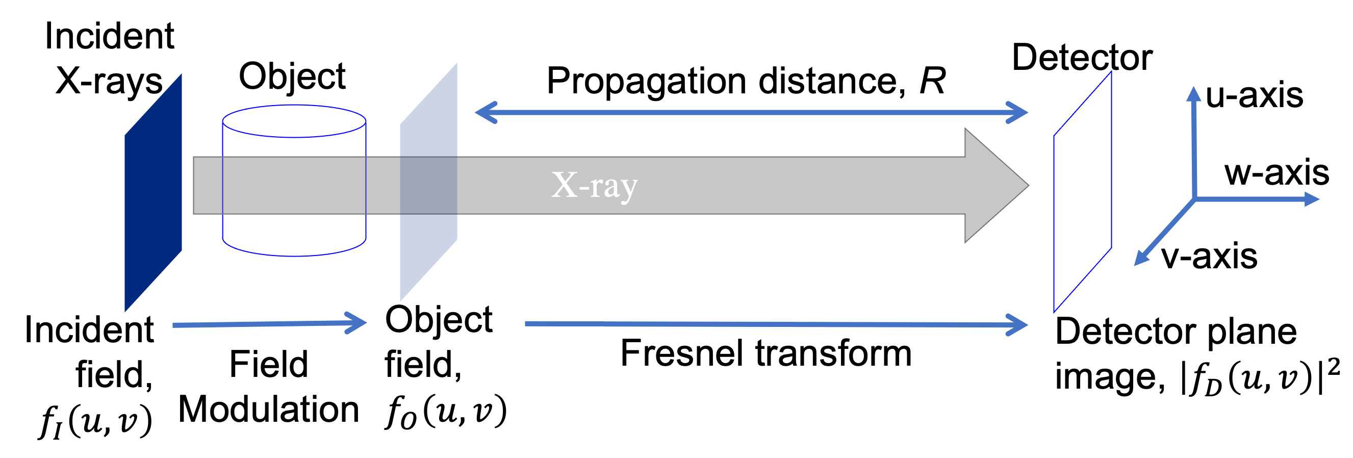
Propagation-based X-ray phase-contrast tomography (XPCT) at synchrotron beamlines is widely used for 3D imaging due to the high-intensity, monochromatic, spatially coherent, and parallel-beam properties of synchrotron X-rays. XPCT is also a popular tool for obtaining higher edge contrast in laboratory micro-focus X-ray CT systems. XPCT is used for 3D reconstruction of a wide variety of objects in biology [1, 2, 3], material science [4, 5, 6, 7, 8], medical imaging [9, 10], and paleontology [11, 12]. In synchrotron XPCT111Henceforth, XPCT refers to XPCT using the monochromatic, parallel, and coherent X-rays at a synchrotron., the object is exposed to a parallel beam of X-rays and the X-ray intensity is recorded by a 2D detector at several rotation angles of the object (Fig. 1). Phase-contrast is a function of the Fresnel number and the phase shift induced by the object on the X-ray field. A detailed discussion of the parameters governing phase-contrast is provided in [13]. In our application (Fig. 1), we adjust the Fresnel number by modifying the propagation distance to achieve adequate phase-contrast in the X-ray images. XPCT can either be performed at a single object-to-detector distance or be repeated at several object-to-detector distances.
The solution to the inverse problem of object reconstruction is a combination of two sequential steps. First, we perform 2D phase-retrieval at each tomographic view to reconstruct the complex-valued images of the transmission X-ray field, in Fig. 1, or its phase shift from the detector images [14, 15]. Henceforth, we shall refer to the phase component of the recovered field as the phase image. Next, we use a tomographic reconstruction algorithm to reconstruct the 3D refractive index decrement of the object from the phase images [16]. In our phase-retrieval algorithms, we reconstruct the 2D phase image at each tomographic view angle from X-ray images at one or more propagation distances. Phase-retrieval is a non-linear inverse problem since it relies on the inversion of a non-linear analytical forward model that relates the phase to the X-ray images. The tomographic reconstruction step is used to reconstruct the 3D refractive index decrement from the retrieved phase images at all the views. Reconstruction of the refractive index decrement from the phase images is a linear inverse problem that is solved using any analytical or iterative CT reconstruction method, including the widely used filtered back projection (FBP) algorithm [16].
The popular choice for phase-retrieval algorithms in XPCT relies on the inversion of forward models that express the measured X-ray images222Or, simple functional forms such as affine and/or logarithm transforms of the X-ray images are expressed as a linear transform of the phase. as a linear transformation of the phase image. For XPCT using X-ray images at a single propagation distance, phase-retrieval reduces to the application of a digital linear filter on the individual X-ray images [14, 17, 18, 19, 20, 21, 22, 23, 24]. These methods also constrain the material composition by approximating the absorption index to be zero or enforcing a proportionality relation between the refractive index decrement and the absorption index. In the case of multi-distance XPCT, phase-retrieval is performed by the inversion of approximate linear relations between the multi-distance X-ray images and the phase [15, 25, 26, 27, 28, 29]. Some of these methods avoid the approximations of zero-absorption and phase-absorption proportionality [28, 29, 15]. Gureyev et al. [30, 31] derives linear analytic formulas for phase-retrieval in the Fresnel region for coherent and partially-coherent radiation. While such linear phase-retrieval (LPR) algorithms are computationally fast, the forward modeling approximations severely restrict the material composition and experimental design. If LPR algorithms are used outside their range of validity, they produce reconstructions with quantitative inaccuracies, false (unwanted) artifacts, and/or image blur.
To address the limitations of linear phase-retrieval (LPR), several non-linear phase-retrieval (NLPR) algorithms have been proposed [32, 33, 34, 35, 36, 37, 38, 39, 40]. The algorithms in [33, 34, 35, 36, 40, 39, 38] reconstruct the phase images with regularization to promote sparsity in projection space. Alternatively, the algorithms in [32, 37] directly reconstruct the 3D object using tomography consistency conditions to improve phase-retrieval by leveraging information from across view angles. While the latter approach is arguably better to constrain the solution space, it is also highly compute intensive while also being difficult to parallel compute. Hence, we pursue the former disjoint approach of phase-retrieval followed by tomographic reconstruction of the object.
NLPR algorithms [32, 33, 34, 35, 36, 37, 38, 39, 40] are generally more accurate than LPR algorithms since they avoid the linear approximations made in the forward measurement model. NLPR estimates the phase images by minimizing a distance measure between the X-ray images and the output of a non-linear forward measurement model. They also use certain sparsity constraints in the form of prior models or regularization functions to limit the solution space for the phase-retrieval problem. The use of such explicit regularization functions requires the user to manually tune one or more parameters to achieve the claimed performance improvements of artifact reduction, improved sharpness, and quantitative accuracy. In contrast, our approach achieves these benefits while avoiding parameter tuning due to the absence of regularization functions. Optionally, our approach also supports implicit constraints in our non-linear forward model that follow directly from the material properties.
In recent years, several deep learning (DL) approaches [41, 42, 43, 44, 45, 46, 47] have also been proposed for phase-retrieval in XPCT. Using DL, the authors demonstrated improved performance without the excessive computational cost of NLPR approaches. However, the limitation of DL approaches is the need for representative training data to train the neural network models. In contrast, both LPR and NLPR algorithms do not require any training data and are broadly applicable to a wide range of objects.
In this paper, we present new non-linear phase-retrieval (NLPR) algorithms for both single-distance and multi-distance XPCT. A limited version of this manuscript with preliminary results was published in the form of a conference proceedings paper [48]. Our NLPR algorithms also support constraints on the material composition. In particular, we demonstrate the use of the phase-absorption proportionality constraint (mathematically equivalent to the single material constraint) for single-distance XPCT. First, we formulate discrete non-linear forward models using the Fresnel transform in Fourier frequency space. This model expresses the measured data as an analytical non-linear function of the phase images. Next, we formulate an objective function that is a measure of the distance between the measured data and the forward model output. Unlike existing non-linear approaches, we do not use prior-models or regularization functions in the objective function to achieve the desired goals of artifact-free, sharp, and accurate reconstructions. Finally, we iteratively solve for the phase images that minimize the objective function while also satisfying any constraint on the material composition.
We initialize our NLPR algorithms with the phase and absorption images that are estimated using LPR algorithms. We perform a comprehensive investigation of initialization strategies by varying the LPR method used for initialization and its regularization parameter. The characteristics and contributions of our proposed NLPR algorithms are -
-
•
Maximum likelihood formulation of phase-retrieval by inversion of non-linear forward measurement models.
-
•
Fresnel propagation based non-linear forward models with optional constraints.
-
•
Phase-retrieval by minimization of non-convex objective functions using the LBFGS algorithm.
-
•
Quantitatively accurate and sharp reconstructions with reduced artifacts compared to LPR approaches.
-
•
Avoids manual tuning of regularization hyper-parameters due to the absence of regularizing prior models.
-
•
Our recommended initialization strategy also avoids hyper-parameter tuning.
-
•
Optional constraints such as single material (homogeneous) object, phase-absorption proportionality, or zero-absorption.
-
•
Open-source software with documentation.
We implemented our algorithms using the PyTorch framework and python programming language. For faster computation, our algorithms can also be run on multiple GPUs. We have released our phase-retrieval software under an open-source license along with documentation at the link https://github.com/phasetorch/phasetorch.
II X-ray Measurement Physics
In this section, we present a mathematical formulation for the physics of measurement in XPCT.
II-A Modulation of the X-ray Field
In XPCT, the measured data is sensitive to the 3D variations in the absorption index, , and refractive index decrement, , of the imaged object. Here, represents the 3D Cartesian coordinate system such that the X-ray propagation is along the axis and perpendicular to the plane. The absorption index and refractive index decrement are expressed compactly as the complex refractive index , where is the imaginary unit.
As X-rays propagate through an object, the X-ray field undergoes a change in both amplitude and phase. The reduction in X-ray intensity after propagation through an object is a direct measure of the object’s absorption index, . The phase shift of the X-ray field that is induced by the object is a direct measure of its refractive index decrement, . Ignoring constant phase terms, the modulated X-ray field, , is expressed as,
| (1) |
where is the complex-valued incident X-ray field, is the transmission function such that , where
| (2) |
Here, is the wavelength of the monochromatic and coherent X-ray field.
II-B Measurement of Fresnel Propagated Field
As the X-ray field propagates from the object to the detector, the phase shifts induced by the object manifest as Fresnel diffraction fringes in the X-ray intensity images that are measured at the detector. The X-ray field at the detector plane, , is expressed as a 2D convolution of the X-ray field at the exit plane, , downstream of the sample and the Fresnel impulse response function, , where is the object to detector distance and is the wavenumber [15, 48, 32]. The X-ray field propagation is depicted in Fig. 1.
The Fresnel transform is more efficiently computed in Fourier frequency space. Let and denote the 2D Fourier transform of the X-ray fields and respectively, where are the 2D Fourier frequency coordinates. Then,
| (3) |
Information on the phase of the X-ray field is lost since detector measurements are only sensitive to the intensity of the X-ray field. Thus, the detector measurements are modeled as, , where is the width of each detector pixel, denotes the magnitude of a complex number, and denote the row and column indices of the detector pixel. The square-root of the normalized detector measurement is then modeled as,
| (4) |
where is the incident X-ray field from equation (1).
III Forward Model
The forward models formulated in this section will be used in the phase-retrieval algorithms that estimate the transmission function from the measurements . To formulate a forward model, we first translate the continuous space expressions in section II to discrete space. Let denote a sampling of the transmission function in equation (1). Let , , and denote the sampled discrete representation of the continuous space X-ray fields , , and respectively333 , , and are a sampling of the X-ray fields , , and in discrete space such that and .. Let , , and represent the discrete Fourier transform (DFT) coefficients of , , and respectively.
III-A Discretization of Measurement Model
We derive the discretized relation between the incident X-ray field and the X-ray field at the exit plane of the object. Given that represents the transmission function in discrete space, we have,
| (5) |
Next, we discretize the relation between the square-root normalized detector measurements in equation (4) and the X-ray field at the exit plane of the object. To sample the Fresnel transform in equation (3), we substitute and , where are the discrete frequency coordinates, is the sampling width along the -axis, and is the sampling width along the -axis. Note that and are the number of discrete coordinates along the -axis and -axis respectively. Thus, a discrete sampling of Fourier space Fresnel transform is given by,
| (6) |
Given equation (6), we can now express the relation between the DFT of and DFT of as,
| (7) |
We use edge padding in the space domain for to avoid circular convolution artifacts. In edge padding, the pixel values along an edge are copied to the neighboring padded regions. Since the detector only measures the intensity of the X-ray field, the square root of the normalized measurement in the absence of noise is expressed as,
| (8) |
where is the discrete X-ray field in the detector plane given by the inverse discrete Fourier transform (IDFT) of and denotes the magnitude of a complex number.
In practice, the noise in detector measurements is modeled using Poisson statistics. Due to the variance stabilizing property of the square root transformation of Poisson random variables [49], we can model the noise statistics of the square root normalized measurement (experimentally determined using equation (25) in the supplementary document) as a Gaussian distribution with constant variance. Thus, the forward model for the square root normalized measurement is given by,
| (9) |
where is additive Gaussian noise with a constant variance for all and .
III-B Non-Linear Forward Models for XPCT
The forward model that relates to is obtained by combining equations (5), (7), and (9). For convenience of notation, we will use matrix-vector notation for mathematical formulation of the forward model in discrete space. In section III-B1, we present a forward model where is unconstrained, which does not impose restrictions on the material composition of the imaged object. In this case, the is a complex valued number that uniquely encodes the X-ray phase shift and total X-ray absorption by the object. In section III-B2, we present a forward model where is constrained, which restricts the material composition of the imaged object. In this case, the feasible solution space of the complex valued is restricted such that it can only be expressed as the function of a real valued . This constraint is useful to restrict the feasible solution space for the phase shift and X-ray absorption.
III-B1 Unconstrained x
Let y, x, and n be column vectors whose elements include a raster ordering of the discrete samples , , and respectively. The matrix H is an operator that when left-multiplied to x returns the Fresnel transform of x. The forward model term computes the magnitude of the IDFT of the Fresnel transform (equation (7)) of the DFT of 444 Note that the matrix H includes the forward and inverse Fourier transform operations in discrete space unlike the continuous space transform in equation (7). . The vector form of the unconstrained forward model is,
| (10) |
where denotes element-wise magnitude. The DFT and IDFT operations are implemented using fast Fourier transform algorithms. Equation (10) expresses the dependence of the real valued measurement vector y on the complex valued transmission vector x.
III-B2 Constrained x
In the absence of data y at multiple propagation distances, unique reconstruction of x is achieved by imposing constraints on the imaged sample. For single-distance XPCT, it is typical to use constraints such as single material [17], phase-absorption proportionality [21], or zero absorption [20]. However, such constraints may introduce inaccuracies and artifacts for objects that do not satisfy these constraints.
The single-material and phase-absorption proportionality constraints are mathematically expressed as,
| (11) |
Alternatively, under the zero-absorption constraint, we have,
| (12) |
The two constraints in equations (11) and (12) are equivalent to expressing the complex valued x in terms of a real valued z such that,
| (13) |
where and are real valued constants that are dependent on the material composition. For the phase-absorption proportionality constraint (equation (11)), we set the ratio of over equal to the ratio of the refractive index decrement to the absorption index . For the zero-absorption constraint in equation (12), we set . We discuss the possible choices for and and the associated trade-offs in section IV-B.
IV Non-Linear Phase-Retrieval (NLPR)
In this section, we will formulate phase-retrieval algorithms using the maximum likelihood (ML) estimation framework. The reconstruction x is such that it minimizes the negative log-likelihood function , which is a measure of the statistical likelihood of the measurement data y given the transmission function x. Under the ML framework, we perform phase-retrieval by solving the optimization problem of . First, we formulate an approach to estimate the unconstrained transmission function x. Next, we present an approach to estimate x such that it also satisfies the constraint in equation (13). Finally, we solve for the X-ray absorption and phase shift at the exit plane of the object from the estimated x. We do not use a prior likelihood model to enforce sparsity in reconstruction of x. Instead, we initialize x using conventional linear phase-retrieval algorithms, which mimics the role of regularization and leads to improved solutions [50].
IV-A Unconstrained NLPR (U-NLPR)
To reconstruct x without any constraints, we utilize X-ray images at several propagation distances. Let denote the square root normalized measurements at a propagation distance of . Then, the negative log-likelihood function is , where is the total number of distances. Here, the noise in each element of is approximated to be additive Gaussian with variance and denotes the squared norm of a vector. Thus, the unconstrained x is estimated by solving the following optimization problem,
| (15) |
We call this approach as unconstrained NLPR (U-NLPR).
IV-B Constrained NLPR (C-NLPR)
Using measurements at a single propagation distance and in the absence of sparsity constraints, it is difficult to independently reconstruct both the phase and absorption of the X-ray field after propagation through the imaged objects. Information on the phase and absorption are entangled in the X-ray intensity measurements. Hence, we impose restrictions on the composition of the object to halve the number of unknowns during phase-retrieval using equation (13).
Let denote the square root normalized measurements at a propagation distance of . Then, the negative log-likelihood function is . We estimate z by solving the following optimization problem,
| (16) |
The complex valued transmission function is then estimated as . This method is called constrained NLPR (C-NLPR).
The scalar constraint parameters of and are dependent on the material composition. They also influence the speed of convergence of C-NLPR. Hence, it is important to intelligently set the parameters of and . For a pure-phase object with zero absorption, we can choose and . However, reconstruction of pure-phase objects will not be investigated in this paper. If a sample is homogeneous, i.e., consists of a single material [17] or satisfies the phase-absorption proportionality constraint [21], then we have several choices for setting and . Let and denote the scalar values of the refractive index decrement and absorption index under these constraints, i.e., we assume .
IV-B1
For this constraint, we set such that from equation (13). From equations (2) and (13), we see that is a discretization of the absolute value for the transmission function . The dynamic range of z is determined by the corresponding dynamic ranges for that is in-turn determined by . For low X-ray absorption materials, if denotes the element of z, then since . The precision of 32-bit floating point numbers becomes progressively inadequate to accurately represent the dynamic range of as it approaches . Hence, may lead to very slow convergence or numerical instabilities at very low values of . Since z is the discretized representation of , is a discretization of only when . Hence, and leads to the parameterization of , which only requires knowledge of the ratio of . This method will be referred to as .
IV-B2
For this constraint, we set such that from equation (13). From equations (2) and (13), we see that is a discretization of the phase component of the transmission function . The dynamic range of z is determined by the corresponding dynamic range of or . For objects with a high refractive index decrement, if denotes the element of z, then if is very large. Hence, may lead to very slow convergence or numerical instabilities for highly refractive materials. Since z is a discretization of , will represent only when . Hence, and leads to the parameterization of , which only requires knowledge of the ratio of . This method will be referred to as .
IV-B3
For this constraint, we control the dynamic range of z depending on the individual known values of and . We set and such that approximately varies between a preset low value of and a high value of . For , we simply choose a value that is greater than but also an order of magnitude less than . In this paper, we choose . Then, the values for and are such that,
-
•
in the absence of any material along the ray path for the pixel.
-
•
when a material with refractive index decrement and absorption index lies along the entirety of the ray.
Ideally, should only vary between and in the absence of measurement non-idealities and a perfect choice for and . In practice, varies approximately within this chosen transmission range, which reduces the risk of numerical instabilities. Thus, our choice for and are,
| (17) | ||||
| (18) |
where is the pixel width. The number of pixels in the X-ray images along the axis and axis are and respectively. However, this particular choice of and requires approximate knowledge of both and . In contrast, the previous two choices that are described in sections IV-B1 and IV-B2 only require knowledge of the ratio . The constraint obtained using equations (17) and (18) will be referred to as (TrOpt indicates optimized transmission).
In section VI, we demonstrate that provides the best trade-off between stable optimization and good performance while only requiring knowledge of the ratio .
IV-C Optimization Algorithm
We implemented our NLPR algorithms using python programming language and PyTorch framework [51]. PyTorch uses algorithmic differentiation (or automatic differentiation) to compute gradients of the objective functions that are used for minimization. In equation (15), algorithmic differentiation is used to compute the gradient of with respect to x. Similarly, algorithmic differentiation is used to compute the gradient of with respect to z in equation (16).
We use the LBFGS algorithm [52, 53] to solve the optimization problems in equations (15) and (16). The gradients computed using algorithmic differentiation are used by the LBFGS optimization algorithm to reconstruct x in (15) and z in (16). In this paper, we use the LBFGS implementation in [54] with a history size of . The maximum number of iterations is capped at and we use Wolfe line search for optimal selection of step-size. We use a convergence criteria that automatically stops the LBFGS iterations based on the convergence of reconstruction and objective function values. We stop LBFGS when the following conditions are met for consecutive iterations,
-
•
Average of the absolute differences in the reconstruction (z in C-NLPR or x in U-NLPR), expressed as a percentage, is less than . The difference is computed between the reconstructions at consecutive two iterations.
-
•
The absolute difference in the objective function ( in C-NLPR or in U-NLPR), expressed as a percentage, is less than .
In this paper, we choose , , and for all the simulated and experimental results in section VI. We recognize that this particular setting for the convergence criteria may appear overly stringent. Our particular choice was designed to ensure sufficient convergence for all data presented in this paper. However, for any given data set, the convergence criteria may be relaxed for reduced run-time.
IV-D Initialization
IV-D1 Multi-distance linear phase-retrieval
The performance of U-NLPR is dependent on the initial estimate for x that is used to initialize the optimization in equation (15). If the phase and absorption in equation (2) are set to zero, then each element of the vector x is .
For multi-distance phase-retrieval using U-NLPR, we show in section VI that zero-initialization for the phase/absorption leads to improved results compared to the state-of-the-art conventional approaches to multi-distance phase-retrieval. However, we also demonstrate that initialization using conventional phase-retrieval methods can further improve the performance of U-NLPR. In this paper, we explore the use of the following phase-retrieval (PR) methods for initialization of U-NLPR.
- 1.
- 2.
- 3.
Unlike U-NLPR, these conventional phase-retrieval methods use a regularization parameter that must be fine-tuned for acceptable performance [15]. The value of this regularization parameter will impact both the performance of the conventional phase-retrieval method used for initialization of U-NLPR and the U-NLPR algorithm. To achieve the best performance for U-NLPR without the need for parameter tuning, we use the Contrast Transfer Function (CTF) phase-retrieval [15] with a sufficiently low value for the regularization given by,
| (19) |
where is a very small value and the term is defined555The terms , , and are defined in [15] and are not related to any terms that are defined in this paper. The regularization parameter in our paper is equivalent to the in equation (14) of the paper [15]. in the reference [15]. In this paper, we set .
As a pre-processing step before running multi-distance phase-retrieval algorithms including U-NLPR, the X-ray images must be registered such that the object appears at the same location in the X-ray images at all the propagation distances.
IV-D2 Single-distance linear phase-retrieval
For single-distance phase-retrieval using C-NLPR, we investigate the use of zero initialization and Paganin PR [17] for the phase images. Paganin PR solves the transport of intensity equation while assuming a single-material object (phase-absorption proportionality).
IV-E Estimation of Phase and Absorption
To perform tomographic reconstruction, we need to estimate discrete sampled representations of and (from equation (2)). Let the vectors A and be the discrete representations of and in raster order.
IV-E1 U-NLPR
The X-ray absorption, , and phase shift, , that is induced by the object on the incident X-ray field is,
| (20) |
where and are the imaginary and real parts of respectively. Here, and 666We use function of numpy [56]. It is the signed angle between the ray from the origin to and the ray from the origin to the point-of-interest. are element-wise vector operators. The phase estimated using U-NLPR is wrapped if the dynamic range for the phase exceeds . Hence, we use phase unwrapping [57, 58] to unwrap the phase images prior to tomographic reconstruction.
IV-E2 C-NLPR
The X-ray absorption and phase images for C-NLPR are computed as,
| (21) |
Since the phase obtained using equation (21) is already unwrapped, we do not need to apply an explicit phase unwrapping procedure.
V Tomographic Reconstruction
In XPCT, measurement data is acquired at several rotation angles of the object. Let and denote the phase and absorption images at view index . The and from equations (20) and (21) are proportional to the projections of the refractive index decrement and absorption index at view . From equation (2), we see that the phase shift and absorption terms divided by the wavenumber are linear projections of the refractive index decrement and absorption index respectively. Filtered back projection (FBP) [16] is a popular algorithm that is widely used for reconstruction of X-ray absorption index from its linear projections. Thus, we use FBP to also reconstruct the refractive index decrement from its linear projections, divided by the wavenumber, at all the views. In this paper, we do not investigate reconstruction of the absorption index.
V-A Low Frequency Information Loss
The reconstruction of refractive index decrement produced by U-NLPR and FBP may contain low frequency artifacts. These artifacts have been well-documented in the research literature [15, 59, 60, 31] on multi-distance phase-retrieval algorithms. Low frequency artifacts refer to slowly varying spurious artifacts in the reconstructions due to the loss of low frequency information in the measurements. Multi-distance phase-retrieval does not use material constraints such as the phase-absorption proportionality. Instead, they rely on measurements at a wide range of propagation distances for inversion.
We will investigate the loss of low frequency information using the transfer function in equation (3). Equation (3) expresses the X-ray field at the detector as a function of the X-ray field at the exit-plane of the object in Fourier space. In the limit as the frequency components and approach zero, we have,
| (22) |
Thus, the value for , in the limit of zero frequencies, does not change with the propagation distance since is a parameter of only the Fresnel transfer function in equation (3). The detector only measures X-ray intensities (equation (4)). To compensate for this loss in phase information, we acquire measurements at varying propagation distances such that the phase-contrast fringes vary in magnitude and thickness. The phase information that is encoded in the phase-contrast fringes can be retrieved by acquiring data at multiple distances. However, since does not vary sufficiently with distance at the low frequencies, we obtain low frequency artifacts in the reconstruction due to insufficient information.
During phase-retrieval, we cannot reconstruct the average value of the phase irrespective of the number of multi-distance measurements. Let us represent the phase as the sum of a constant and a zero-mean phase term , i.e.,
| (23) |
The constant phase term factors out as the scalar multiple in equations (1) and (3). Since the square root normalized measurements in equation (4) measure only the X-ray intensity, information on is lost since is a multiplying factor for .
|
|
|
|
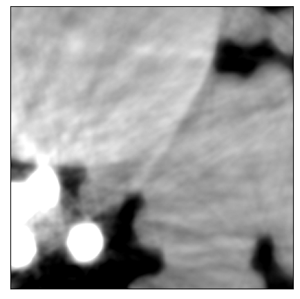
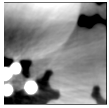
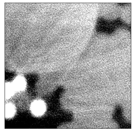
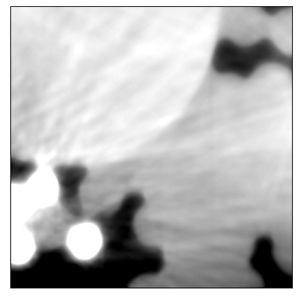
| (a) Single-Material | (b) Single-Material | (c) Multi-Material | (d) Multi-Material |
| axial slice | axial slice | axial slice | axial slice |
|
|
|
|
| (e) Single-Material | (f) Multi-Material | (g) Multi-Material | (h) Multi-Material |
| X-ray image | X-ray image | X-ray image | X-ray image |
 |
 |
| (a) NRMSE vs. Regularization of Conventional PR | (b) SSIM vs. Regularization of Conventional PR |
| Multi-distance Phase-Retrieval (PR) followed by FBP Reconstruction of the Multi-Material Object | ||||
 |
 |
 |
 |
 |
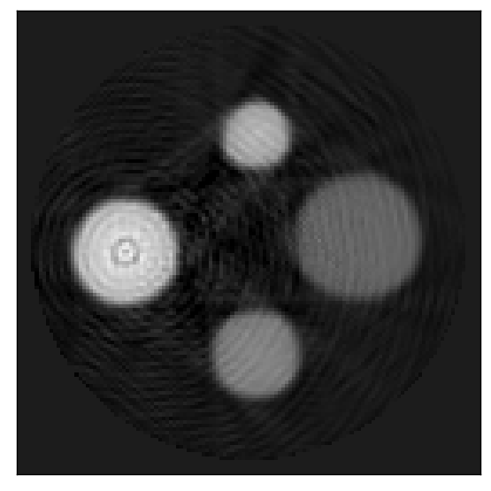
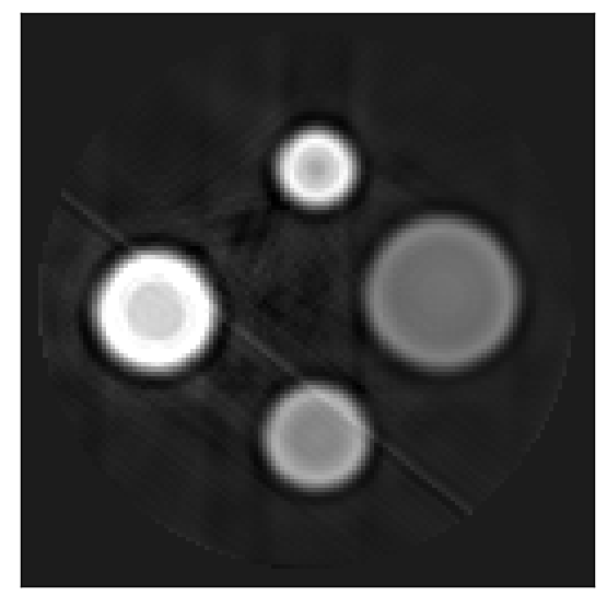
| (a) TIE | (b) CTF | (c) Mixed | (d) U-NLPR/Zero-Initial | (e) U-NLPR/CTF-Initial |
|
|
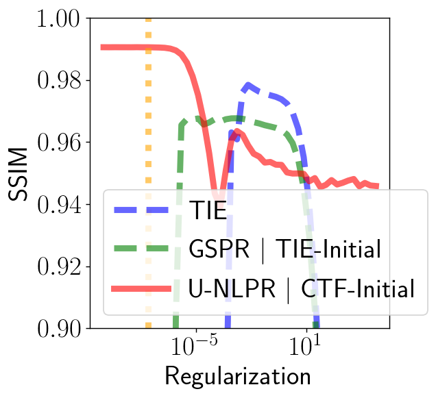
| (a) GSPR TIE-Initial | (b) SSIM vs. Regularization |
| Single Distance PR + FBP of Single-Material Object | Single Distance PR + FBP of Multi-Materials | |||
 |
 |
 |
 |
 |
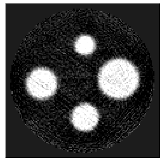
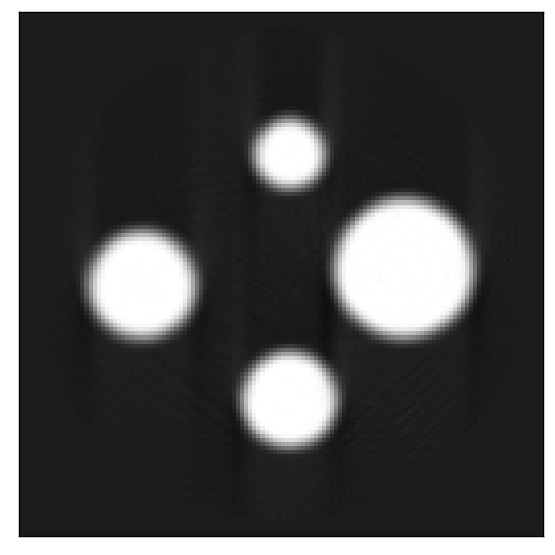
| (a) Paganin | (b) C-NLPR/0-Initial | (c) C-NLPR/Pag-Initial | (d) Paganin | (e) C-NLPR/Pag-Initial |
|
|
|---|---|
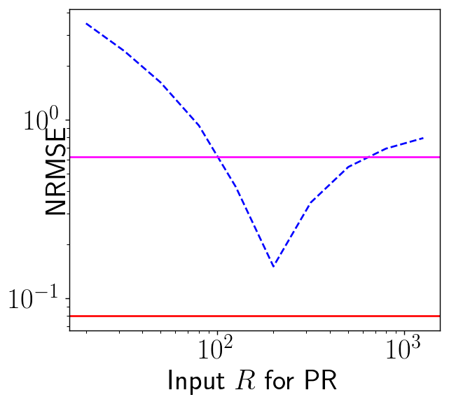
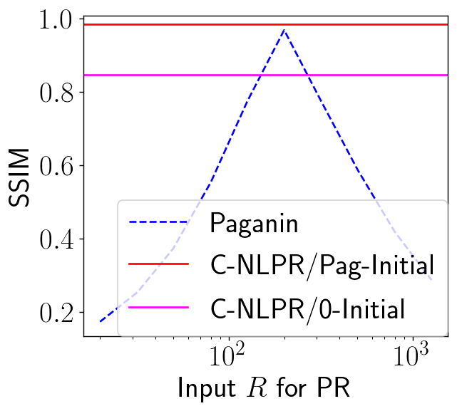
| (a) NRMSE | (b) SSIM |
 |
 |
 |
 |
| (a) RMSE/SSIM | (b) True- | (c) High- | (d) Low- |
 |
 |
 |
 |
 |
| (a) CTF | (b) TIE | (c) Mixed | (d) U-NLPR/0-Initial | (e) U-NLPR/CTF-Initial |
 |
 |
 |
 |
 |
| (f) CTF | (g) TIE | (h) Mixed | (i) U-NLPR/0-Initial | (j) U-NLPR/CTF-Initial |
 |
 |
 |
 |
 |
| (k) CTF | (l) TIE | (m) Mixed | (n) U-NLPR/0-Initial | (o) U-NLPR/CTF-Initial |
 |
 |
 |
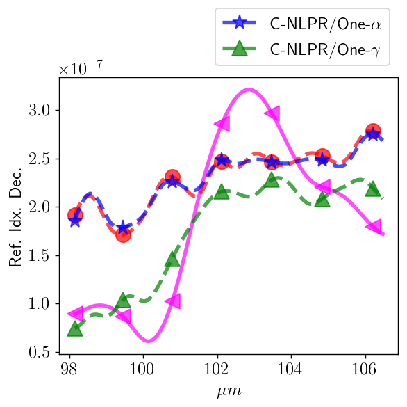 |
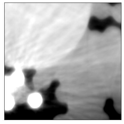
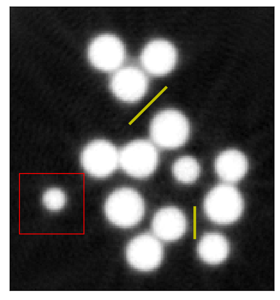
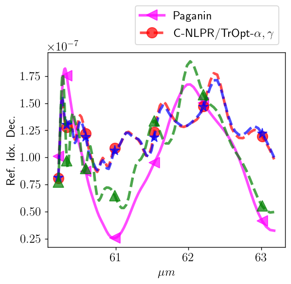
| (a) Paganin PR | (b) C-NLPR/One- | (c) Top Line Profile | (d) Bottom Line Profile |
 |
 |
 |
|
| (e) Paganin PR Zoomed | (f) C-NLPR/One- Zoomed | (g) Modulation Transfer Function (MTF) | |
|
| (a) Objective and run time |
|
| (b) % change in and z |
V-B Quantitative Evaluation
Our approach to extracting quantitative information from the refractive index decrement reconstructions is to compare the reconstructed values for the material-of-interest with the reconstructed values of the background air. We assume that the theoretical refractive index decrement of the background air is . Unfortunately, this process of quantitative evaluation cannot be automated since determination of the background air region is non-trivial and application dependent. First, we compute the average value of the reconstruction in the background, denoted as . Next, we compute the average value of the reconstruction inside the material-of-interest, denoted as . Finally, we compute the background subtracted refractive index decrement of the material-of-interest as,
| (24) |
Background subtraction is necessary due to the loss of the average value for the refractive index in the reconstruction. After background subtraction, is the quantitatively accurate refractive index decrement that is comparable to the theoretical values.
VI Results
VI-A Simulated Data
In this section, we compare the performance of our new NLPR algorithms against existing approaches using simulated phase-contrast CT data of a 3D object at a monochromatic X-ray energy of . To avoid using the same forward model for both simulation and inversion, we simulate X-ray images from finely sampled objects at very high resolutions using equation (8). The simulated phase-contrast CT data, the stack of X-ray images over all views, is then sub-sampled to a size of by block-averaging the simulated images over non-overlapping square-shaped windows of pixels. Finally, we simulate Poisson-like noise in the measurements by adding zero-mean Gaussian noise with a standard deviation that is of the simulated data (equation (9)).
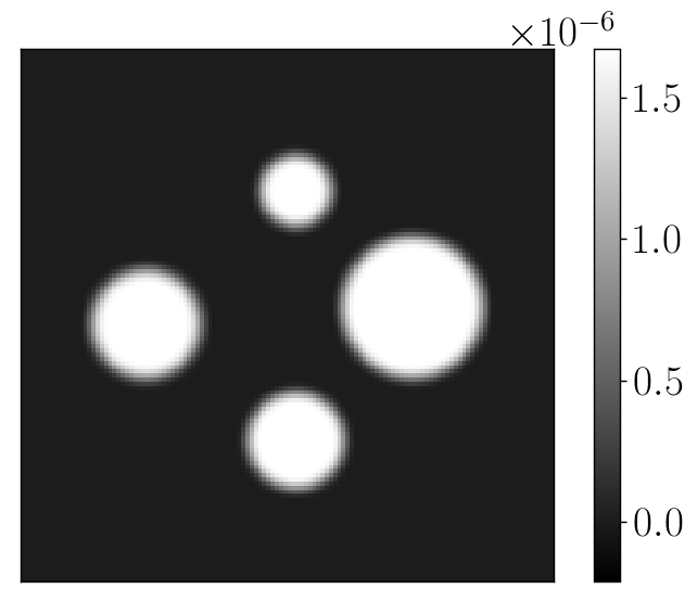
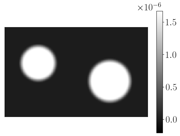
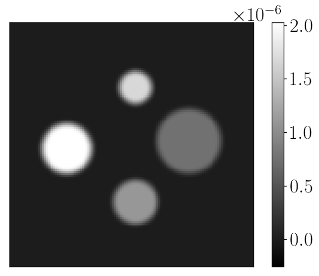
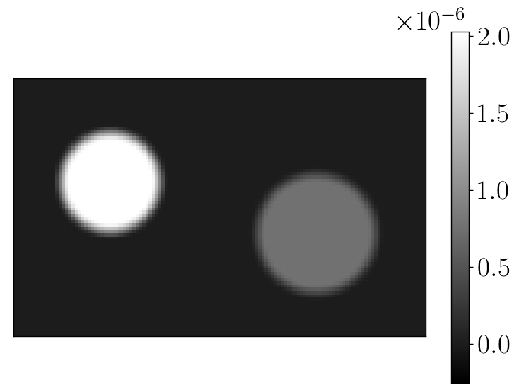
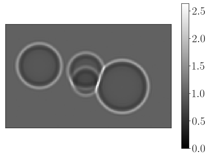
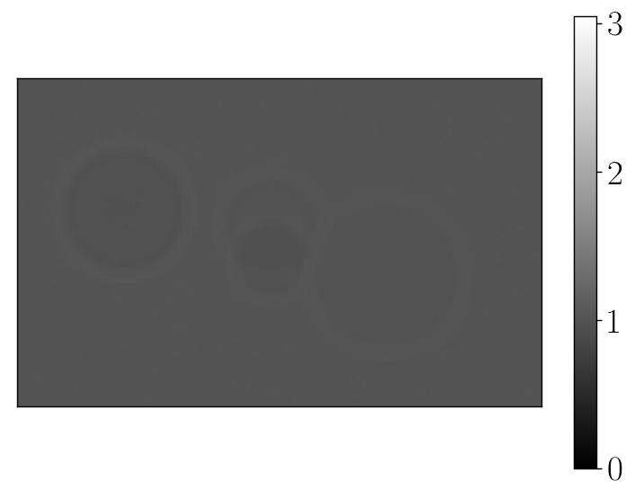
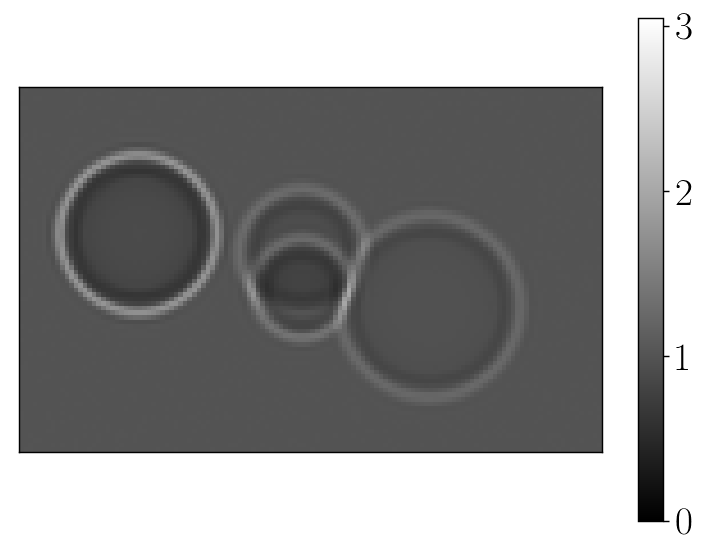
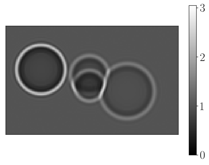
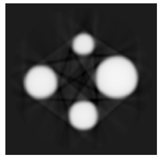
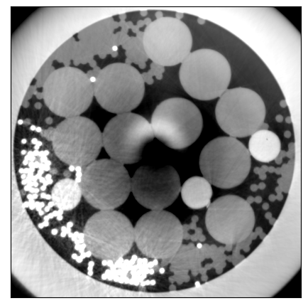
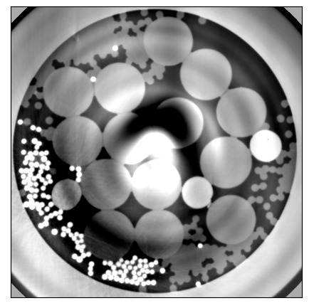
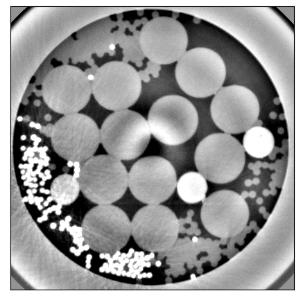
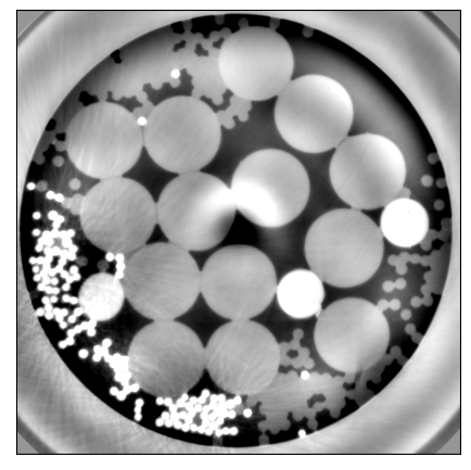
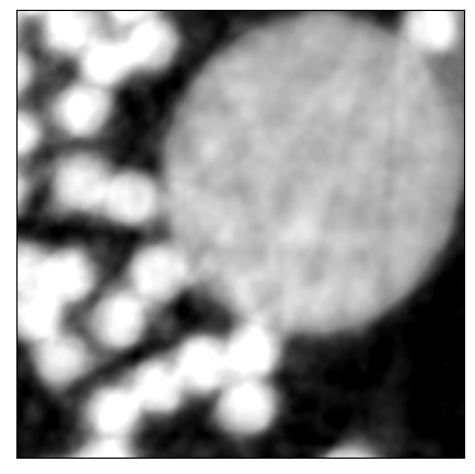
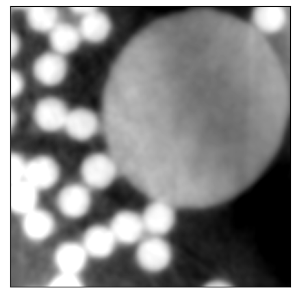
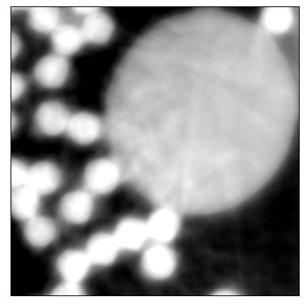
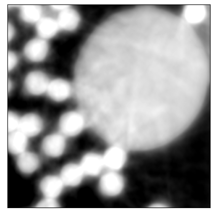
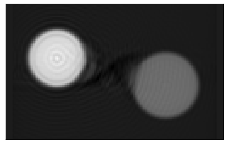
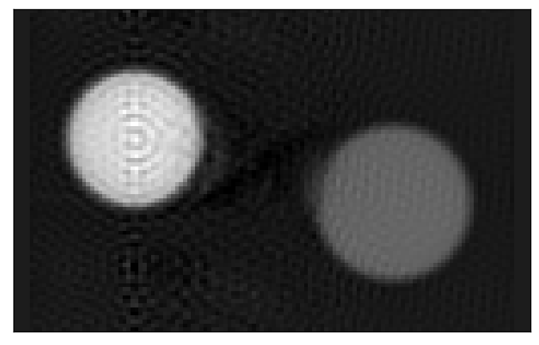
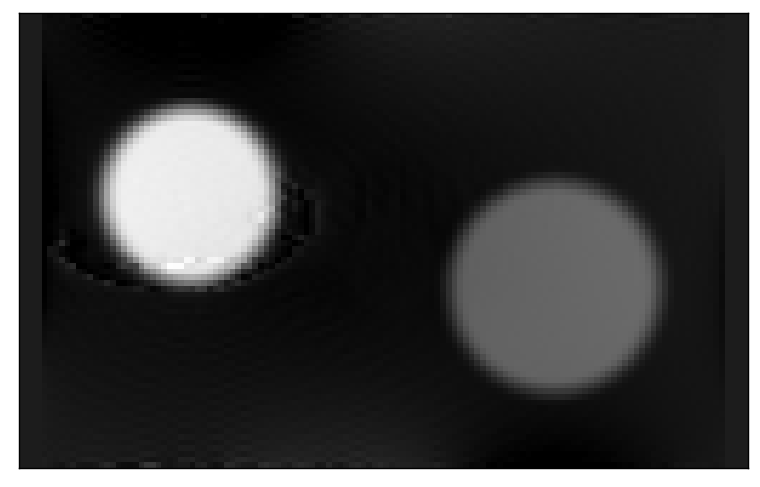
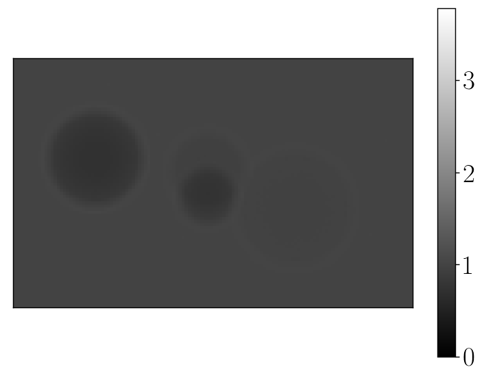
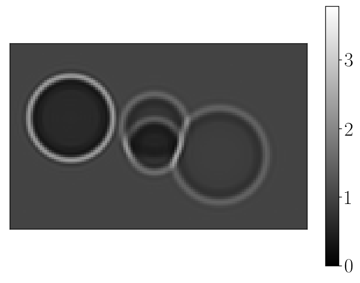
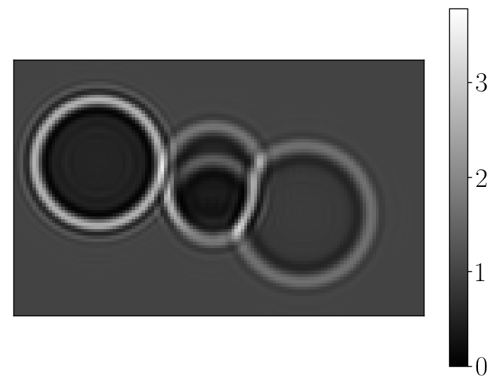
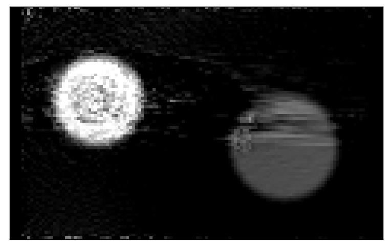
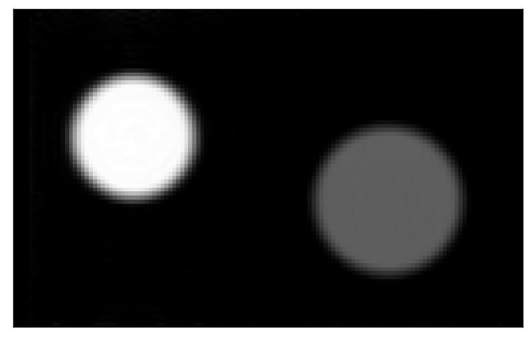
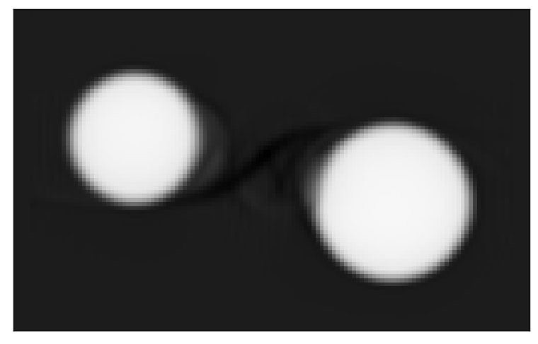
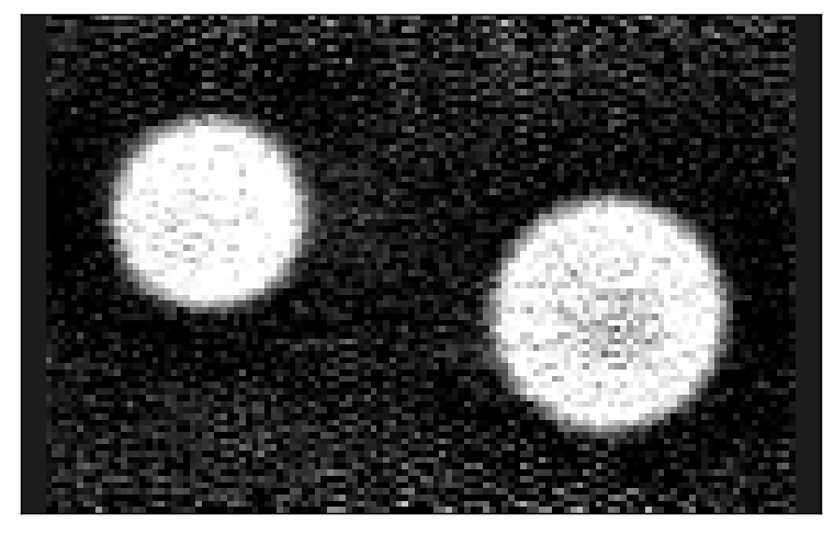
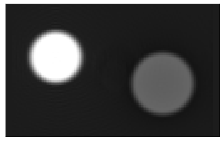
Cross-sectional slices through the simulated object along with the corresponding simulated X-ray images with phase-contrast are shown in Fig. 2. First, we simulate a single-material object (Fig. 2 (a, b)) that consists of several spheres with differing diameters but made using the same material. The material used for the spheres is SiC with a refractive index decrement () of and absorption index () of at an X-ray energy of . For this object, the normalized X-ray image with phase-contrast at a propagation distance of is shown in Fig. 2 (e). Next, we simulate a multi-material object (Fig. 2 (c, d)) that consists of four spheres with varying diameters and differing atomic composition. For the spheres, we chose SiC (), Teflon (), Alumina (), and Polyimide () as the materials. The X-ray images with phase-contrast for this heterogeneous object are shown in Fig. 2 (f-h) at propagation distances, , of , , and . For both the single and multi-material objects, the radii of the spheres were chosen to be , , , and respectively. We simulate X-ray images of size with pixel width of at tomographic views equally spaced over an angular range of . For phase-retrieval (PR), we use the square root of the normalized X-ray images (equation (25) in supplementary document).
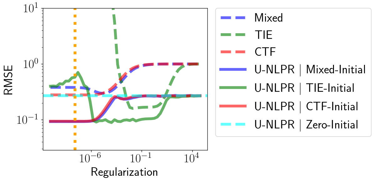
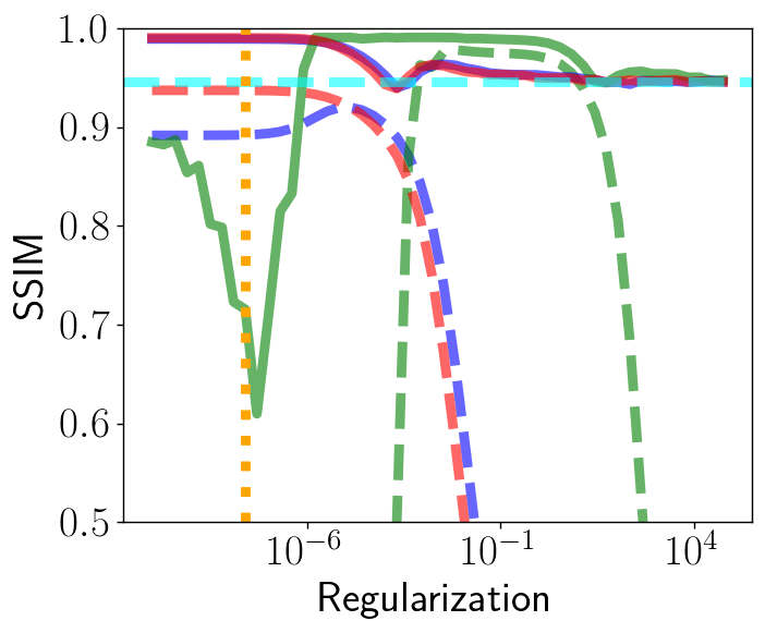
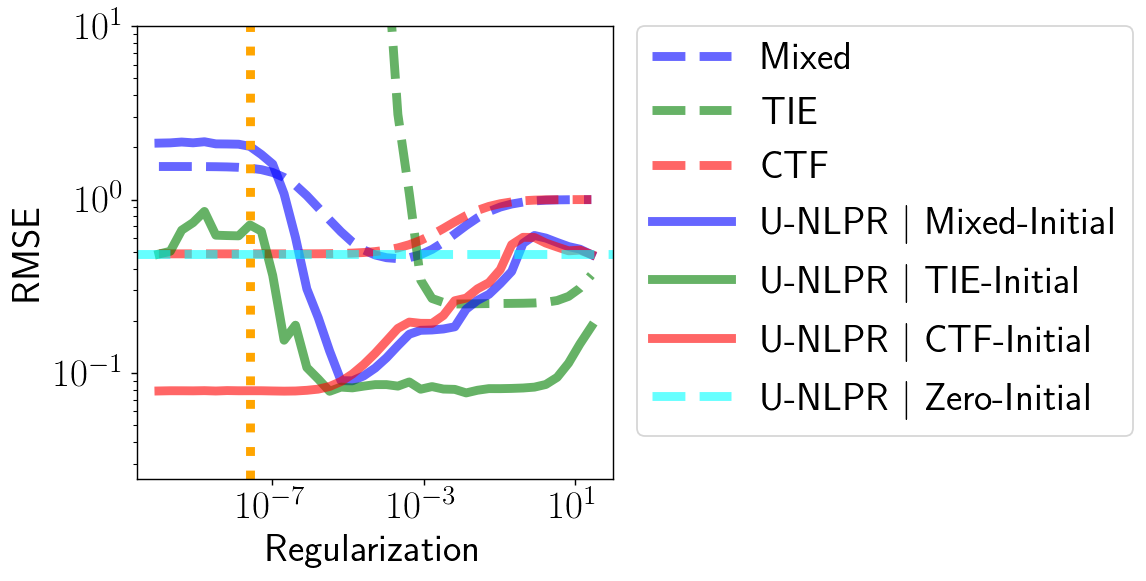
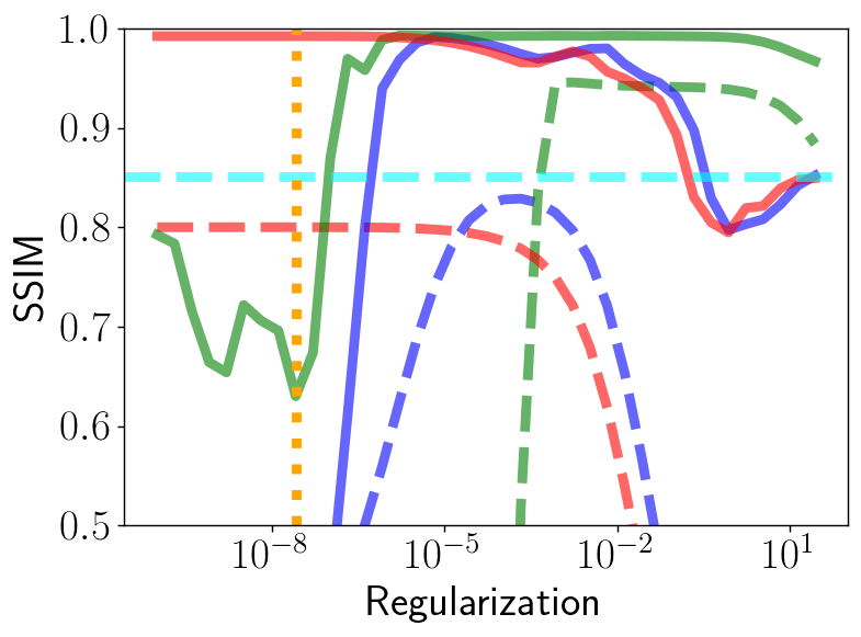
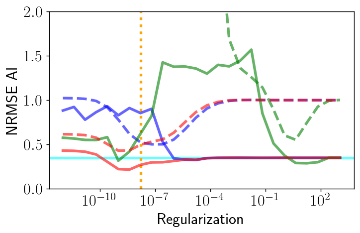
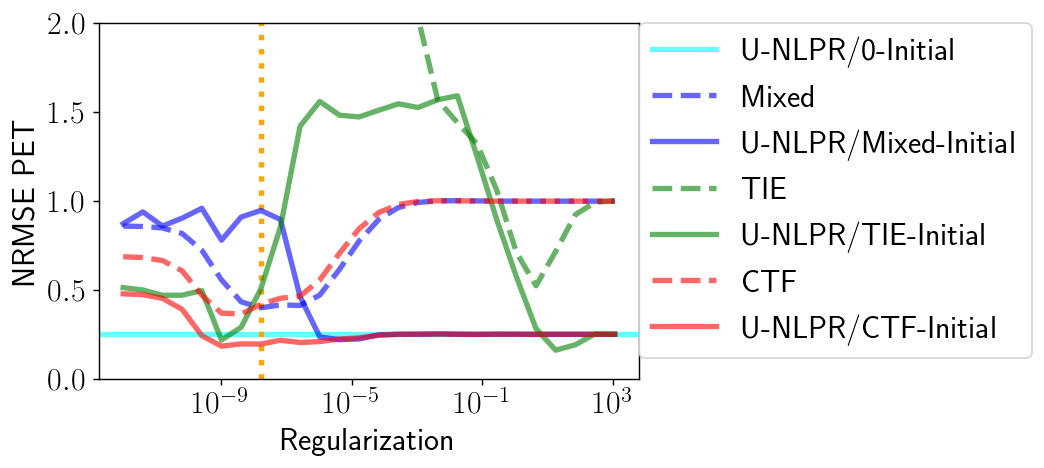
A quantitative comparison of the refractive index decrement reconstructions using various multi-distance phase-retrieval algorithms is presented in Fig. 3. At each tomographic view, we use phase-retrieval to estimate the phase images that are a measure of the phase shift induced by the object on the X-ray field. Then, we use filtered back projection (FBP) to perform a tomographic reconstruction of the refractive index decrement from the phase images. Fig. 3 (a) is the normalized root mean squared error (NRMSE)777NRMSE is normalized using the averaged norm of the ground-truth. between the reconstructions and the ground-truth. Fig. 3 (b) is the structural similarity index measure (SSIM)888For SSIM, the inputs are linearly scaled such that the minimum and maximum values of ground-truth are mapped to and respectively. We use Gaussian weights with standard deviation of pixels.. We use the NRMSE and SSIM implementations from scikit-image [58]. We compute NRMSE and SSIM for the entire volume of the spheres after background subtraction as described in the section V-B. For the conventional phase-retrieval methods [15, 28, 29] of CTF, TIE, and Mixed, we plot (dashed lines) the NRMSE and SSIM measures as a function of its regularization parameter. To adequately reduce NRMSE and increase SSIM using TIE phase-retrieval, we must carefully tune its regularization hyper-parameter to lie within a narrow range of parameter values. An arbitrary choice of either a very low or high parameter value for regularization will lead to sub-optimal results with TIE. For CTF and Mixed phase-retrieval, it is possible to achieve low NRMSE and high SSIM by choosing a sufficiently small value for the regularization. As the regularization parameter is reduced, the performance of CTF does not degrade while Mixed leads to a marginal reduction in performance. For CTF, we can minimize the NRMSE and maximize SSIM by choosing a sufficiently small fixed value for the regularization parameter. In particular, we fix the regularization parameter value using equation (19) to avoid the need for parameter tuning.
We use U-NLPR from section IV-A for multi-distance phase-retrieval without any material constraints. The performance of U-NLPR is influenced by the estimates of the phase and absorption that is used for initialization of the optimization in equation (15). In Fig. 3, we investigate the use of phase images from CTF, TIE, or Mixed phase-retrieval as initial estimates for initialization of U-NLPR. The performance of these conventional methods is dependent on the chosen value of the regularization parameter. In Fig. 3, we plot (solid lines) the NRMSE and SSIM for U-NLPR as a function of the regularization parameter of the conventional method (i.e., CTF, TIE, and Mixed) used for initialization. We observe that U-NLPR always produces lower NRMSE and higher SSIM when compared to the estimates from the method used for initialization. Importantly, we observe that the best performance of U-NLPR is achieved by initialization using the CTF algorithm with a sufficiently low value for the regularization as specified in equation (19). While the Mixed approach may also be suitable for initialization, we prefer the CTF approach due to the ease of choosing the regularization using equation (19). Note that the SSIM with Mixed PR decreases slightly at very low regularization values.
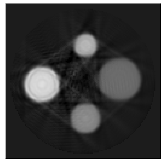
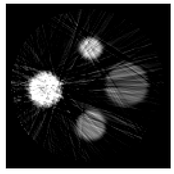
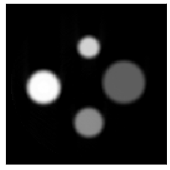
The reconstructions at the optimal regularization with the highest SSIM using the conventional phase-retrieval algorithms of TIE, CTF, and Mixed approaches are shown in Fig. 4 (a-c). While such an optimal selection is perhaps an unfair advantage to the conventional algorithms, we did this to compare against the best possible reconstructions. In Fig. 4 (d), we show the reconstruction using U-NLPR that is initialized with zero values for the phase and absorption. In Fig. 4 (e), we show the U-NLPR reconstruction that is initialized using CTF phase-retrieval that used the regularization of equation (19). Since U-NLPR does not use any regularization, we avoid the need for the tedious manual tuning of regularization hyper-parameters. From Fig. 4 (a-c) and Fig. 2 (c), we observe that conventional phase-retrieval methods produce spurious streak artifacts. While the artifacts are faint in the case of TIE, both CTF and Mixed produce strong streak artifacts. When initialized with zeros for the phase and absorption, U-NLPR in Fig. 4 (d) produce a better reconstruction with significantly fewer streak artifacts than the conventional methods. When initialized using CTF with the fixed regularization of equation (19), U-NLPR produces the best reconstruction with reduced artifacts as shown in Fig. 4 (e).
We also compared our U-NLPR algorithm with a composite approach that uses TIE phase-retrieval followed by a Gerchberg-Saxton phase-retrieval (GSPR) algorithm in Fig. 5. While GSPR [50, 61] is primarily used for far-field diffraction imaging, it has also been successfully applied for imaging in the Fresnel region. Fig. 5 (a) is the refractive index reconstruction using GSPR and TIE initialization. We observe artifacts that are similar to Fresnel diffraction fringes in Fig. 5 (a). U-NLPR with CTF initialization at the regularization from equation (19) has higher SSIM than GSPR at any regularization.
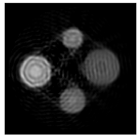
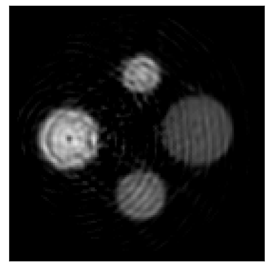
We visually compare the tomographic reconstruction performance of single-distance phase-retrieval algorithms in Fig. 6. Qualitative comparisons of phase-retrieval methods for single-material object and multi-material objects are shown in Fig. 6 (a-c) and Fig. 6 (d, e) respectively. Paganin phase-retrieval [17] produces streak artifacts as shown in Fig. 6 (a, d). We investigate the performance of C-NLPR from section IV-B for non-linear phase-retrieval using the single-material constraint. If C-NLPR is initialized with zeros for the phase images, C-NLPR reduces artifacts but significantly enhances the noise in Fig. 6 (b). C-NLPR using Paganin phase-retrieval for initialization provides the best quality reconstruction as shown in Fig. 6 (c, e). We use the C-NLPR/One- method from section IV-B1 in Fig. 6. Surprisingly, we also observe that the qualitative performance does not degrade for the multi-material object.
Fig. 7 shows a quantitative analysis of the reconstruction performance for various single-distance phase-retrieval algorithms. With Paganin phase-retrieval, it is common to achieve sharper reconstructions by artificially lowering the propagation distance, , that is input to the algorithm. However, from Fig. 7, we see that an inaccurate setting for compared to its true value leads to sub-optimal NRMSE and SSIM values. The best performance for Paganin is achieved when is set equal to the true propagation distance of . Initializing C-NLPR with Paganin phase-retrieved images results in the lowest NRMSE and highest SSIM among all approaches. However, initializing C-NLPR with zero phase images produces sub-optimal reconstructions with large amounts of noise as shown in Fig. 6 (b). In Fig. 6 and Fig. 7, we used the C-NLPR/One- method described in section IV-B1.
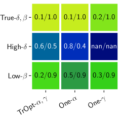
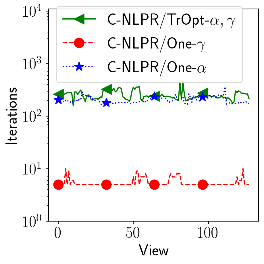
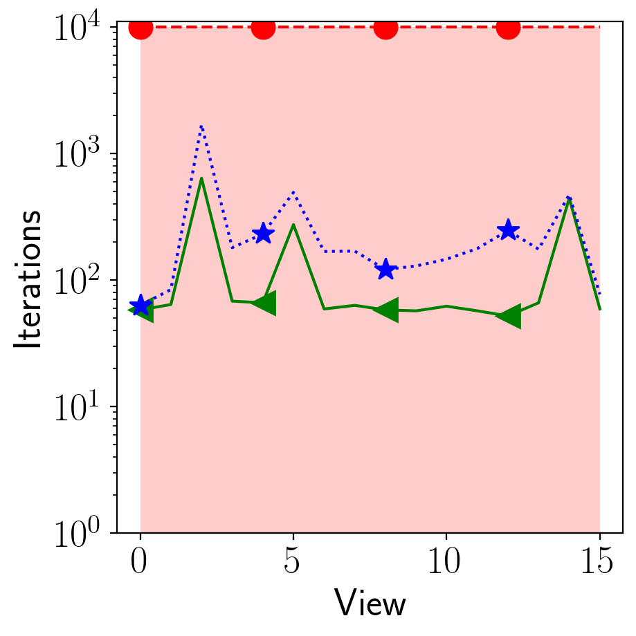
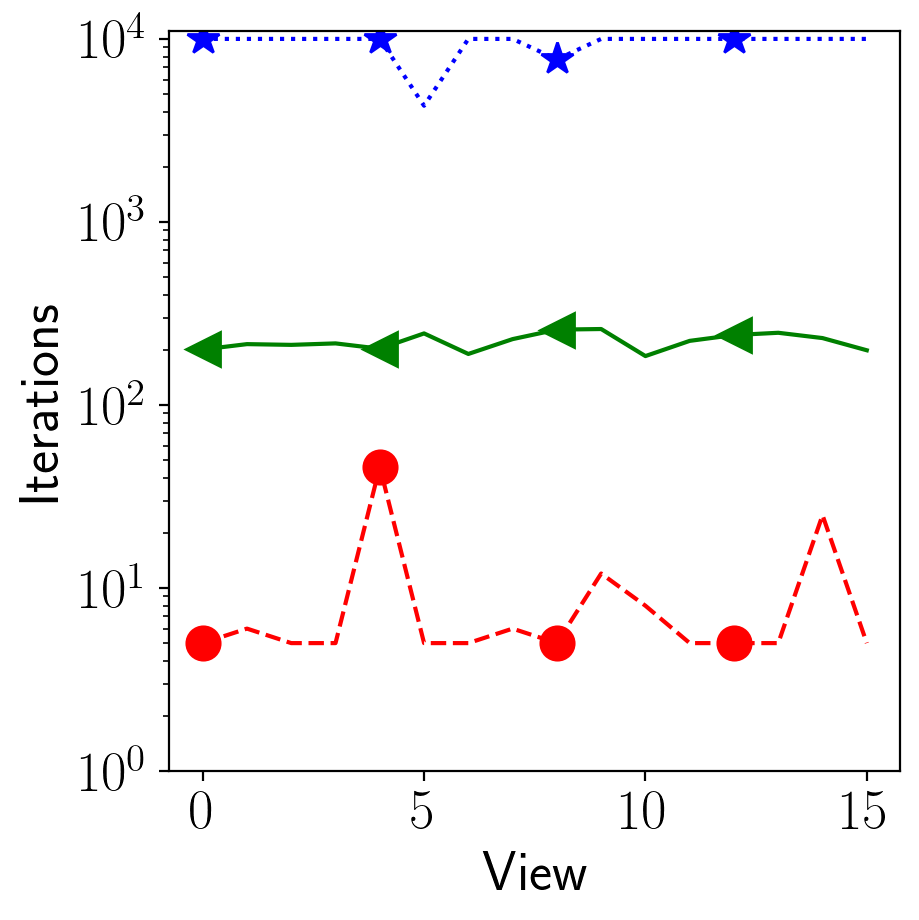
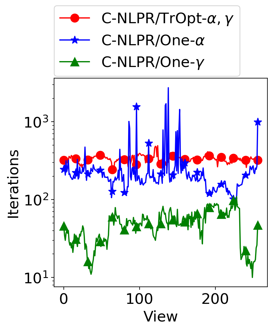
The convergence speed and reconstruction quality of C-NLPR are strongly influenced by the choice of and as evidenced in Fig. 8. Fig. 8 (a) compares the NRMSE and SSIM for different constraint choices of C-NLPR/TrOpt- (section IV-B3), C-NLPR/One- (section IV-B1), and C-NLPR/One- (section IV-B2). The rows of Fig. 8 (a) correspond to different choices for the material properties of while the columns cycle through the various settings used for imposing the single-material constraint. The row label “True-” indicates that the simulated object used the true values for SiC at . The label “High-” indicates a very large value for that is higher than the of SiC. The label “Low-” indicates a very low value for that is the of SiC. For the various materials characterized by its values, we see that C-NLPR/TrOpt- consistently produces the lowest NRMSE. Using the SSIM measure, the results are a tie between C-NLPR/TrOpt- and C-NLPR/One-. However, the latter only uses knowledge of the ratio .
In Fig. 8 (b-d), we plot the number of iterations for the LBFGS optimization algorithm as a function of the tomographic view index. Fig. 8 (b), Fig. 8 (c), and Fig. 8 (d) are plots of the number of iterations (to meet our convergence criteria) for “True-”, “High-”, and “Low-” respectively. For the true values of of SiC, C-NLPR/One- has the fastest convergence in Fig. 8 (b) but increased NRMSE in the first row of Fig. 8 (a). In contrast, both C-NLPR/TrOpt- and C-NLPR/One- converge slower but achieve lower NRMSE. From Fig. 8 (c) and second row of Fig. 8 (a), we see that numerical instabilities associated with C-NLPR/One- result in slow convergence and corrupted reconstructions due to the high value (see section IV-B2). From Fig. 8 (c), C-NLPR/One- is slow to converge and has a high NRMSE as indicated in the third row of Fig. 8 (a) (see section IV-B1). The maximum number of iterations was fixed at for the LBFGS optimization. While C-NLPR/TrOpt- has the best convergence for all cases, it requires knowledge of both and . Alternatively, C-NLPR/One- only uses knowledge of the ratio while also matching C-NLPR/TrOpt- in convergence speed for “True-” and “High-”. Our recommendation is to use C-NLPR/One- since it achieves the best overall performance while only requiring knowledge of the ratio . Here, our objective is primarily to select feasible and values that impact the convergence speed of the algorithm. Thus, small errors in the ratio of or the individual values of are inconsequential. Only an order-of-magnitude change in will have a noticeable impact on convergence.
VI-B Experimental Data
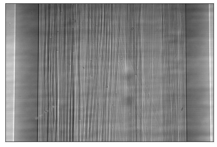
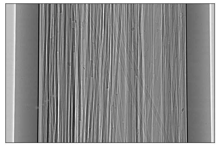
For comparison of phase-retrieval methods using experimental data, a bundle of fibers comprising PolyEthylene Terephthalate (PET), PolyPropylene (PP), Aluminum (), and Aluminum Oxide () with respective diameters of , , , and were enclosed in a borosilicate capillary glass and scanned for tomography at the X-ray imaging beamline 8.3.2 of the Advanced Light Source, Berkeley, California. Monochromator was set to deliver X-ray beam with energy of . A PCO edge camera combined with lens was used to collect X-ray images, resulting in an effective pixel size of approximately . A total number of X-ray images were recorded over range and using a exposure time. The object was placed at approximately from the X-ray source and the detector was placed at object-to-detector propagation distances of , , and for each scan. The size of each X-ray image was . The normalized X-ray images are shown in Fig. S6 of the supplementary document.
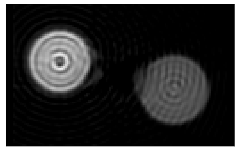
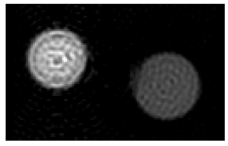
Tomographic reconstructions of the refractive index decrement from phase images reconstructed using various multi-distance phase-retrieval algorithms are shown in Fig. 9. The regularization parameters for the conventional phase-retrieval methods of CTF, TIE, and Mixed are manually tuned to obtain the best visual quality of reconstructions. Substantial low frequency reconstruction artifacts are observed in Fig. 9 (a, b, g, l) for CTF and TIE phase-retrieval. Mixed phase-retrieval produces large amounts of reconstruction noise as shown in the zoomed images of Fig. 9 (h, m). We note that the noise with Mixed can be reduced by adjusting the regularization but it also severely reduces the quality of reconstruction. U-NLPR produces the best reconstructions in Fig. 9 (d, e, i, j, n, o) that substantially reduces both low frequency artifacts and noise when compared to the conventional methods. Surprisingly, U-NLPR with zero-initialization results in a similar level of reconstruction quality as U-NLPR that is initialized using CTF with regularization from equation (19). Note that some of the artifacts in the centers of Fig. 9 (a-e) are ring artifacts [62] and we do not explore the correction of ring artifacts in this paper. The complicated interaction between ring-artifact removal and phase-retrieval algorithms necessitate further investigation. Fig. S7 in the supplementary document presents a quantitative comparison of the phase-retrieval performance.
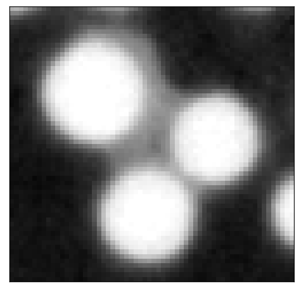
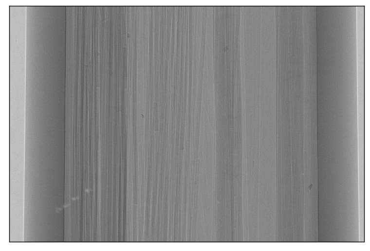
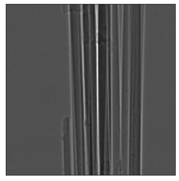
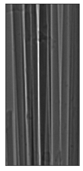
For comparison of single-distance phase-retrieval algorithms, we obtained experimental X-ray CT data with phase-contrast from the Advanced Light Source (ALS) Beamline 8.3.2. CT data of SiC fibers was acquired at an object-to-detector distance of and X-ray energy of . The size of each X-ray image was and the pixel width was . X-ray images were acquired at different views equally spaced over an angular range of degrees. A normalized X-ray image is shown in Fig. S8 of the supplementary document.
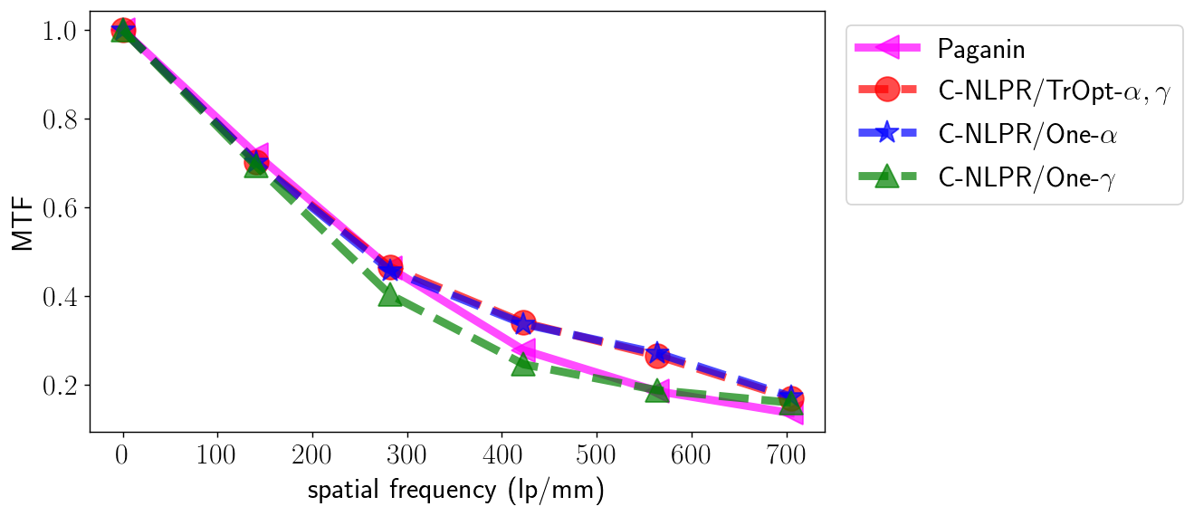
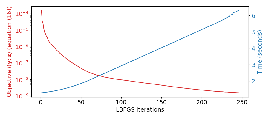
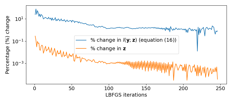
Tomographic reconstructions of the refractive index decrement from phase images reconstructed using various single-distance phase-retrieval algorithms are shown in Fig. 10. Fig. 10 (a, e) and (b, f) show the reconstructions using Paganin and C-NLPR/One- respectively. The line profiles in Fig. 10 (c, d) are along the yellow lines in Fig. 10 (a, b). They highlight the reduction in streak artifacts using C-NLPR/One- when compared to Paganin phase-retrieval. The zoomed images in Fig. 10 (e, f) also demonstrate the significant enhancement in sharpness using C-NLPR/One- even in the presence of a second material that is not modeled by the constraints of C-NLPR. Fig. 10 (g) is a plot of the modulation transfer function (MTF) [63] that indicates sharper reconstructions from C-NLPR/One- and C-NLPR/TrOpt-. A convergence analysis for the reconstructions in Fig. 10 is shown in Fig. 11. Fig. 11 (a) is a plot of the time elapsed and the objective function as a function of the LBFGS iterations. Fig. 11 (b) is a plot of the percentage change in the objective function and the estimated values as a function of the iteration number. The total time for phase-retrieval at one view was seconds on a NVIDIA Tesla V100 GPU.
VII Conclusion
For propagation-based X-ray phase-contrast tomography (XPCT), we presented new non-linear phase-retrieval algorithms (NLPR) to reconstruct the phase shift induced by the object on the X-ray field. Then, we demonstrated reconstruction of the refractive index decrement in 3D from the phase shift images using tomographic reconstruction algorithms. Our approaches do not require any manual tuning of image quality related hyper-parameters such as regularization. Our NLPR algorithms are suitable for both single-distance and multi-distance XPCT while also supporting constraints on the material composition. For single-distance XPCT, we demonstrated phase-retrieval (PR) under the constraint of single-material or phase-absorption proportionality. Our NLPR algorithms produced the best reconstructions based on both quantitative metrics of accuracy as well as qualitative evaluation of artifact and noise reduction. The superior performance of NLPR is a result of employing non-linear measurement models that are more accurate than the linear approximate models used by existing linear PR approaches. For multi-distance XPCT, we show that zero-initialization of the phase for NLPR may be sufficient, but the best performance is achieved by initializing with the Contrast Transfer Function (CTF) PR. For single-distance XPCT, we show that NLPR produces the best reconstruction when initialized with Paganin PR.
Acknowledgments
LLNL-JRNL-847272. This work was performed under the auspices of the U.S. Department of Energy by Lawrence Livermore National Laboratory under Contract DE-AC52-07NA27344. LDRD 22-ERD-011 was used to fund the research in this paper. This research used resources of the Advanced Light Source, which is a DOE Office of Science User Facility under contract no. DE-AC02-05CH11231.
References
- [1] C. Karunakaran, R. Lahlali, N. Zhu, A. M. Webb, M. Schmidt, K. Fransishyn, G. Belev, T. Wysokinski, J. Olson, D. M. L. Cooper, and E. Hallin, “Factors influencing real time internal structural visualization and dynamic process monitoring in plants using synchrotron-based phase contrast X-ray imaging,” Scientific Reports, vol. 5, no. 1, Jul. 2015.
- [2] L. C. P. Croton, K. S. Morgan, D. M. Paganin, L. T. Kerr, M. J. Wallace, K. J. Crossley, S. L. Miller, N. Yagi, K. Uesugi, S. B. Hooper, and M. J. Kitchen, “In situ phase contrast X-ray brain CT,” Scientific Reports, vol. 8, no. 1, Jul. 2018.
- [3] S. Wilkins, T. E. Gureyev, D. Gao, A. Pogany, and A. Stevenson, “Phase-contrast imaging using polychromatic hard x-rays,” Nature, vol. 384, no. 6607, pp. 335–338, 1996.
- [4] L. Zielke, C. Barchasz, S. Waluś, F. Alloin, J.-C. Leprêtre, A. Spettl, V. Schmidt, A. Hilger, I. Manke, J. Banhart, R. Zengerle, and S. Thiele, “Degradation of Li/S Battery Electrodes On 3D Current Collectors Studied Using X-ray Phase Contrast Tomography,” Scientific Reports, vol. 5, no. 1, p. 10921, Jun. 2015.
- [5] N. D. Parab, Z. A. Roberts, M. H. Harr, J. O. Mares, A. D. Casey, I. E. Gunduz, M. Hudspeth, B. Claus, T. Sun, K. Fezzaa, S. F. Son, and W. W. Chen, “High speed X-ray phase contrast imaging of energetic composites under dynamic compression,” Applied Physics Letters, vol. 109, no. 13, p. 131903, Sep. 2016.
- [6] F. Sun, L. Zielke, H. Markötter, A. Hilger, D. Zhou, R. Moroni, R. Zengerle, S. Thiele, J. Banhart, and I. Manke, “Morphological Evolution of Electrochemically Plated/Stripped Lithium Microstructures Investigated by Synchrotron X-ray Phase Contrast Tomography,” ACS Nano, vol. 10, no. 8, pp. 7990–7997, Aug. 2016.
- [7] D. S. Eastwood, P. M. Bayley, H. Jung Chang, O. O. Taiwo, J. Vila-Comamala, D. J. L. Brett, C. Rau, P. J. Withers, P. R. Shearing, C. P. Grey, and P. D. Lee, “Three-dimensional characterization of electrodeposited lithium microstructures using synchrotron X-ray phase contrast imaging,” Chemical Communications, vol. 51, no. 2, pp. 266–268, 2015.
- [8] S. C. Mayo, T. J. Davis, T. E. Gureyev, P. R. Miller, D. Paganin, A. Pogany, A. W. Stevenson, and S. Wilkins, “X-ray phase-contrast microscopy and microtomography,” Optics express, vol. 11, no. 19, pp. 2289–2302, 2003.
- [9] S. Pacilè, P. Baran, C. Dullin, M. Dimmock, D. Lockie, J. Missbach-Guntner, H. Quiney, M. McCormack, S. Mayo, D. Thompson, Y. Nesterets, C. Hall, K. Pavlov, Z. Prodanovic, M. Tonutti, A. Accardo, J. Fox, S. Tavakoli Taba, S. Lewis, P. Brennan, D. Hausermann, G. Tromba, and T. Gureyev, “Advantages of breast cancer visualization and characterization using synchrotron radiation phase-contrast tomography,” Journal of Synchrotron Radiation, vol. 25, no. 5, pp. 1460–1466, Sep. 2018.
- [10] A. Bravin, P. Coan, and P. Suortti, “X-ray phase-contrast imaging: from pre-clinical applications towards clinics,” Physics in Medicine and Biology, vol. 58, no. 1, pp. R1–R35, Dec. 2012.
- [11] V. Fernandez, E. Buffetaut, E. Maire, J. Adrien, V. Suteethorn, and P. Tafforeau, “Phase Contrast Synchrotron Microtomography: Improving Noninvasive Investigations of Fossil Embryos In Ovo,” Microscopy and Microanalysis, vol. 18, no. 1, pp. 179–185, Feb. 2012.
- [12] E. M. Friis, P. R. Crane, K. R. Pedersen, S. Bengtson, P. C. J. Donoghue, G. W. Grimm, and M. Stampanoni, “Phase-contrast X-ray microtomography links Cretaceous seeds with Gnetales and Bennettitales,” Nature, vol. 450, no. 7169, Nov. 2007.
- [13] T. E. Gureyev, Y. I. Nesterets, A. W. Stevenson, P. R. Miller, A. Pogany, and S. W. Wilkins, “Some simple rules for contrast, signal-to-noise and resolution in in-line x-ray phase-contrast imaging,” Optics express, vol. 16, no. 5, pp. 3223–3241, 2008.
- [14] A. Burvall, U. Lundström, P. A. C. Takman, D. H. Larsson, and H. M. Hertz, “Phase retrieval in X-ray phase-contrast imaging suitable for tomography,” Optics Express, vol. 19, no. 11, pp. 10 359–10 376, May 2011.
- [15] M. Langer, P. Cloetens, J.-P. Guigay, and F. Peyrin, “Quantitative comparison of direct phase retrieval algorithms in in-line phase tomography,” Medical Physics, vol. 35, no. 10, pp. 4556–4566, 2008.
- [16] A. C. Kak and M. Slaney, Principles of Computerized Tomographic Imaging. Society of Industrial and Applied Mathematics, 2001.
- [17] D. Paganin, S. C. Mayo, T. E. Gureyev, P. R. Miller, and S. W. Wilkins, “Simultaneous phase and amplitude extraction from a single defocused image of a homogeneous object,” Journal of Microscopy, vol. 206, no. 1, 2002.
- [18] M. A. Beltran, D. M. Paganin, K. Uesugi, and M. J. Kitchen, “2D and 3D X-ray phase retrieval of multi-material objects using a single defocus distance,” Optics Express, vol. 18, no. 7, pp. 6423–6436, Mar. 2010.
- [19] T. E. Gureyev, T. J. Davis, A. Pogany, S. C. Mayo, and S. W. Wilkins, “Optical phase retrieval by use of first Born- and Rytov-type approximations,” Applied Optics, vol. 43, no. 12, p. 2418, Apr. 2004.
- [20] A. V. Bronnikov, “Reconstruction formulas in phase-contrast tomography,” Optics Communications, vol. 171, no. 4, pp. 239–244, Dec. 1999.
- [21] X. Wu, H. Liu, and A. Yan, “X-ray phase-attenuation duality and phase retrieval,” Opt. Lett., vol. 30, no. 4, pp. 379–381, Feb 2005.
- [22] R. C. Chen, L. Rigon, and R. Longo, “Comparison of single distance phase retrieval algorithms by considering different object composition and the effect of statistical and structural noise,” Opt. Express, vol. 21, no. 6, pp. 7384–7399, Mar 2013. [Online]. Available: https://opg.optica.org/oe/abstract.cfm?URI=oe-21-6-7384
- [23] R. Chen, H. Xie, L. Rigon, R. Longo, E. Castelli, and T. Xiao, “Phase retrieval in quantitative x-ray microtomography with a single sample-to-detector distance,” Optics Letters, vol. 36, no. 9, pp. 1719–1721, 2011.
- [24] D. M. Paganin, V. Favre-Nicolin, A. Mirone, A. Rack, J. Villanova, M. P. Olbinado, V. Fernandez, J. C. da Silva, and D. Pelliccia, “Boosting spatial resolution by incorporating periodic boundary conditions into single-distance hard-x-ray phase retrieval,” Journal of Optics, vol. 22, no. 11, p. 115607, 2020.
- [25] B. Yu, L. Weber, A. Pacureanu, M. Langer, C. Olivier, P. Cloetens, and F. Peyrin, “Evaluation of phase retrieval approaches in magnified X-ray phase nano computerized tomography applied to bone tissue,” Optics Express, vol. 26, no. 9, pp. 11 110–11 124, Apr. 2018.
- [26] S. Zabler, P. Cloetens, J.-P. Guigay, J. Baruchel, and M. Schlenker, “Optimization of phase contrast imaging using hard x rays,” Review of Scientific Instruments, vol. 76, no. 7, p. 073705, Jul. 2005.
- [27] M. Langer, P. Cloetens, and F. Peyrin, “Regularization of Phase Retrieval With Phase-Attenuation Duality Prior for 3-D Holotomography,” IEEE Transactions on Image Processing, vol. 19, no. 9, pp. 2428–2436, Sep. 2010.
- [28] P. Cloetens, W. Ludwig, E. Boller, L. Helfen, L. Salvo, R. Mache, and M. Schlenker, “Quantitative phase contrast tomography using coherent synchrotron radiation,” in Developments in X-Ray Tomography III, vol. 4503. SPIE, Jan. 2002, pp. 82–91.
- [29] J. P. Guigay, M. Langer, R. Boistel, and P. Cloetens, “Mixed transfer function and transport of intensity approach for phase retrieval in the Fresnel region,” Optics Letters, vol. 32, no. 12, p. 1617, Jun. 2007.
- [30] T. Gureyev, Y. Nesterets, D. Paganin, A. Pogany, and S. Wilkins, “Linear algorithms for phase retrieval in the fresnel region. 2. partially coherent illumination,” Optics Communications, vol. 259, no. 2, pp. 569–580, 2006. [Online]. Available: https://www.sciencedirect.com/science/article/pii/S0030401805010357
- [31] T. Gureyev, A. Pogany, D. Paganin, and S. Wilkins, “Linear algorithms for phase retrieval in the fresnel region,” Optics Communications, vol. 231, no. 1, pp. 53–70, 2004. [Online]. Available: https://www.sciencedirect.com/science/article/pii/S0030401803023320
- [32] K. A. Mohan, X. Xiao, and C. A. Bouman, “Direct model-based tomographic reconstruction of the complex refractive index,” in 2016 IEEE International Conference on Image Processing (ICIP), Sep. 2016, pp. 1754–1758.
- [33] V. Davidoiu, B. Sixou, M. Langer, and F. Peyrin, “Non-linear iterative phase retrieval based on Frechet derivative,” Optics Express, vol. 19, no. 23, p. 22809, Nov. 2011.
- [34] ——, “Non-linear iterative phase retrieval based on Frechet derivative and projection operators,” in 2012 9th IEEE International Symposium on Biomedical Imaging (ISBI), May 2012, pp. 106–109.
- [35] ——, “Nonlinear Phase Retrieval Using Projection Operator and Iterative Wavelet Thresholding,” IEEE Signal Processing Letters, vol. 19, no. 9, pp. 579–582, Sep. 2012.
- [36] ——, “Nonlinear approaches for the single-distance phase retrieval problem involving regularizations with sparsity constraints,” Applied Optics, vol. 52, no. 17, p. 3977, Jun. 2013.
- [37] A. Ruhlandt, M. Krenkel, M. Bartels, and T. Salditt, “Three-dimensional phase retrieval in propagation-based phase-contrast imaging,” Phys. Rev. A, vol. 89, p. 033847, Mar 2014. [Online]. Available: https://link.aps.org/doi/10.1103/PhysRevA.89.033847
- [38] J. Moosmann, R. Hofmann, A. V. Bronnikov, and T. Baumbach, “Nonlinear phase retrieval from single-distance radiograph,” Opt. Express, vol. 18, no. 25, pp. 25 771–25 785, Dec 2010. [Online]. Available: https://opg.optica.org/oe/abstract.cfm?URI=oe-18-25-25771
- [39] K. Mom, M. Langer, and B. Sixou, “Nonlinear primal–dual algorithm for the phase and absorption retrieval from a single phase contrast image,” Opt. Lett., vol. 47, no. 20, pp. 5389–5392, Oct 2022. [Online]. Available: https://opg.optica.org/ol/abstract.cfm?URI=ol-47-20-5389
- [40] S. Maretzke, M. Bartels, M. Krenkel, T. Salditt, and T. Hohage, “Regularized newton methods for x-ray phase contrast and general imaging problems,” Opt. Express, vol. 24, no. 6, pp. 6490–6506, Mar 2016. [Online]. Available: https://opg.optica.org/oe/abstract.cfm?URI=oe-24-6-6490
- [41] K. Mom, M. Langer, and B. Sixou, “Deep gauss-newton for phase retrieval,” Opt. Lett., vol. 48, no. 5, pp. 1136–1139, Mar 2023.
- [42] Y. Wu, L. Zhang, S. Guo, L. Zhang, F. Gao, M. Jia, and Z. Zhou, “Enhanced phase retrieval via deep concatenation networks for in-line x-ray phase contrast imaging,” Physica Medica, vol. 95, pp. 41–49, 2022.
- [43] R. Deshpande, A. Avachat, F. J. Brooks, and M. A. Anastasio, “Investigating the robustness of a deep learning-based method for quantitative phase retrieval from propagation-based x-ray phase contrast measurements under laboratory conditions,” Physics in Medicine & Biology, 2023.
- [44] F. Li, Y. Zhao, S. Han, D. Ji, Y. Li, M. Zheng, W. Lv, J. Jian, X. Zhao, and C. Hu, “Physics-informed deep neural network reconstruction framework for propagation-based x ray phase-contrast computed tomography with sparse-view projections,” Opt. Lett., vol. 47, no. 16, pp. 4259–4262, Aug 2022.
- [45] X. Wu, Z. Wu, S. C. Shanmugavel, H. Z. Yu, and Y. Zhu, “Physics-informed neural network for phase imaging based on transport of intensity equation,” Opt. Express, vol. 30, no. 24, pp. 43 398–43 416, Nov 2022.
- [46] S. Z. Li, M. G. French, K. M. Pavlov, and H. T. Li, “Shallow U-Net deep learning approach for phase retrieval in propagation-based phase-contrast Imaging,” in Developments in X-Ray Tomography XIV, B. Müller and G. Wang, Eds., vol. 12242, International Society for Optics and Photonics. SPIE, 2022, p. 122421Q.
- [47] Y. Zhang, M. A. Noack, P. Vagovic, K. Fezzaa, F. Garcia-Moreno, T. Ritschel, and P. Villanueva-Perez, “Phasegan: a deep-learning phase-retrieval approach for unpaired datasets,” Opt. Express, vol. 29, no. 13, pp. 19 593–19 604, Jun 2021. [Online]. Available: https://opg.optica.org/oe/abstract.cfm?URI=oe-29-13-19593
- [48] K. A. Mohan, D. Y. Parkinson, and J. A. Cuadra, “Constrained Non-Linear Phase Retrieval for Single Distance Xray Phase Contrast Tomography,” Electronic Imaging, vol. 2020, no. 14, pp. 146–1–146–8, Jan. 2020.
- [49] N. L. Johnson, A. W. Kemp, and S. Kotz, Univariate discrete distributions. John Wiley & Sons, 2005, vol. 444.
- [50] T. Gureyev, “Composite techniques for phase retrieval in the fresnel region,” Optics Communications, vol. 220, no. 1, pp. 49–58, 2003. [Online]. Available: https://www.sciencedirect.com/science/article/pii/S0030401803013531
- [51] A. Paszke, S. Gross, F. Massa, A. Lerer, J. Bradbury, G. Chanan, T. Killeen, Z. Lin, N. Gimelshein, L. Antiga, A. Desmaison, A. Kopf, E. Yang, Z. DeVito, M. Raison, A. Tejani, S. Chilamkurthy, B. Steiner, L. Fang, J. Bai, and S. Chintala, “Pytorch: An imperative style, high-performance deep learning library,” in Advances in Neural Information Processing Systems 32. Curran Associates, Inc., 2019, pp. 8024–8035.
- [52] D. C. Liu and J. Nocedal, “On the limited memory bfgs method for large scale optimization,” Mathematical programming, vol. 45, no. 1-3, pp. 503–528, 1989.
- [53] J. Nocedal, “Updating quasi-newton matrices with limited storage,” Mathematics of computation, vol. 35, no. 151, pp. 773–782, 1980.
- [54] H.-J. M. Shi and D. Mudigere, “PyTorch-LBFGS: A PyTorch implementation of L-BFGS,” https://github.com/hjmshi/PyTorch-LBFGS, 2018.
- [55] D. Paganin and K. A. Nugent, “Noninterferometric phase imaging with partially coherent light,” Physical review letters, vol. 80, no. 12, p. 2586, 1998.
- [56] C. R. Harris, K. J. Millman, S. J. van der Walt, R. Gommers, P. Virtanen, D. Cournapeau, E. Wieser, J. Taylor, S. Berg, N. J. Smith, R. Kern, M. Picus, S. Hoyer, M. H. van Kerkwijk, M. Brett, A. Haldane, J. F. del Río, M. Wiebe, P. Peterson, P. Gérard-Marchant, K. Sheppard, T. Reddy, W. Weckesser, H. Abbasi, C. Gohlke, and T. E. Oliphant, “Array programming with NumPy,” Nature, vol. 585, no. 7825, pp. 357–362, Sep. 2020.
- [57] M. A. Herráez, D. R. Burton, M. J. Lalor, and M. A. Gdeisat, “Fast two-dimensional phase-unwrapping algorithm based on sorting by reliability following a noncontinuous path,” Applied Optics, vol. 41, no. 35, p. 7437, Dec. 2002.
- [58] S. van der Walt, J. L. Schönberger, J. Nunez-Iglesias, F. Boulogne, J. D. Warner, N. Yager, E. Gouillart, T. Yu, and the scikit-image contributors, “scikit-image: image processing in Python,” PeerJ, vol. 2, p. e453, 6 2014.
- [59] M. Langer, P. Cloetens, B. Hesse, H. Suhonen, A. Pacureanu, K. Raum, and F. Peyrin, “Priors for X-ray in-line phase tomography of heterogeneous objects,” Philosophical Transactions of the Royal Society A: Mathematical, Physical and Engineering Sciences, vol. 372, no. 2010, p. 20130129, Mar. 2014. [Online]. Available: https://royalsocietypublishing.org/doi/10.1098/rsta.2013.0129
- [60] J. C. Petruccelli, L. Tian, and G. Barbastathis, “The transport of intensity equation for optical path length recovery using partially coherent illumination,” Optics Express, vol. 21, no. 12, pp. 14 430–14 441, Jun. 2013. [Online]. Available: https://www.osapublishing.org/oe/abstract.cfm?uri=oe-21-12-14430
- [61] J. R. Fienup, “Phase retrieval algorithms: a comparison,” Applied optics, vol. 21, no. 15, pp. 2758–2769, 1982.
- [62] K. A. Mohan, S. V. Venkatakrishnan, J. W. Gibbs, E. B. Gulsoy, X. Xiao, M. De Graef, P. W. Voorhees, and C. A. Bouman, “TIMBIR: A Method for Time-Space Reconstruction From Interlaced Views,” IEEE Transactions on Computational Imaging, vol. 1, no. 2, pp. 96–111, Jun. 2015.
- [63] E. Committee, ASTM E1695-95 Standard Test Method for Measurement of Computed Tomography (CT) System Performance. ASTM International, 1995.
VIII Supplementary Material
VIII-A Data Normalization
Bright-field (a.k.a. flat-field) and dark-field measurements are acquired to appropriately normalize the CT scans. Bright-field refers to measurements made with the X-ray beam but without the object and dark-field refers to measurements made in the absence of the X-ray beam. Typically, bright-field measurements are made at the same propagation distances as used for the phase-contrast CT scans.
For normalization, we make certain simplifying approximations on that also serve to simplify the subsequent problem of phase-retrieval. First, we approximate the incident field as a plane wave with constant phase. Without loss of generality, we assume that this constant phase is zero since any information on constant phase terms is lost (equation (4)). Next, we normalize the detector measurements using the bright- and dark-fields. Lastly, we compute the square root of the normalized detector image before running the algorithms presented in section IV. Let and denote the bright-field and dark-field measurements respectively. If denotes the detector image with the object, the square root of the normalized detector image is given by,
| (25) |
Here, is a measure of and is a measure of .
VIII-B Simulated Data
VIII-B1 Multi-distance phase-retrieval
Fig. S1 is a continuation of the results from Fig. 4. The simulation scenario for Fig. S1 and Fig. 4 are described in section VI-A. It demonstrates the superior reconstruction performance of U-NLPR compared to the conventional PR approaches along the slice of the refractive index decrement reconstructions.
For an analysis of the reconstruction performance using simulated data with a higher degree of non-linearity, we simulate phase-contrast images at propagation distances of , , and as shown in Fig. S2. This simulation is for a multi-material object with the same refractive indices as SiC, Teflon, Alumina, and Polymide, but with higher absorption indices for the corresponding materials. From Fig. S3 and Fig. S4, we conclude that U-NLPR with CTF initialization is the best performing reconstruction without any artifacts (for reference, ground-truth images are shown in Fig. 2). It also avoids tuning of the regularization parameter by using the pre-determined regularization from equation (19).
VIII-B2 Single-distance phase-retrieval
Fig. S5 is a continuation of the results in Fig. 6. It demonstrates the superior reconstruction performance of C-NLPR with Paganin initialization along the slice of the refractive index reconstructions.
| Multi-distance Phase-Retrieval (PR) followed by FBP Reconstruction (continued from Fig. 4) | ||||
 |
 |
 |
 |

|
| (a) TIE | (b) CTF | (c) Mixed | (d) U-NLPR/Zero-Initial | (e) U-NLPR/CTF-Initial |
|
|
|
|---|---|---|
| (a) | (b) | (c) |
| axial slice of the second multi-material object using multi-distance phase-retrieval | ||||
 |
 |
 |
 |
|
| (a) TIE | (b) CTF | (c) Mixed | (d) U-NLPR/Zero-Initial | (e) U-NLPR/CTF-Initial |
| axial slice of the second multi-material object using multi-distance phase-retrieval | ||||
 |
 |
 |
 |
|
| (f) TIE | (g) CTF | (h) Mixed | (i) U-NLPR/Zero-Initial | (j) U-NLPR/CTF-Initial |
 |
 |
| (a) NRMSE vs. Regularization of Conventional PR | (b) SSIM vs. Regularization of Conventional PR |
| Single Distance PR + FBP of Single-Material Object | Single Distance PR + FBP of Multi-Materials | |||
 |
 |
 |
 |
 |
| (a) Paganin | (b) C-NLPR/0-Initial | (c) C-NLPR/Pag-Initial | (d) Paganin | (e) C-NLPR/Pag-Initial |
|
|
|
|---|---|---|
| (a) | (b) | (c) |
 |
 |
|
|
|---|---|
| (a) | (b) /Zoomed |
|
|
|
|---|---|
| (a) | (b) |
VIII-C Experimental Data
VIII-C1 Multi-Distance Phase-Retrieval
The discussion in this section is continued from section VI-B. Fig. S6 shows the X-ray images for the multi-material experimental sample. For quantitative analysis of the reconstructions, we compare the normalized root mean squared error (NRMSE) for Al and PET fibers in Fig. S7. The NRMSE is computed only using the reconstructed values in the regions within the Al and PET fibers shown in Fig. S7 that also exclude the edges of each fiber. Importantly, to facilitate comparison with the theoretical values, we use background subtraction for the reconstructed values as explained in section V-B. From the dashed plots in Fig. S7, we can see that choosing a suitable regularization for the conventional phase-retrieval methods is challenging due to the narrow range of parameters with best performance. As the regularization for CTF phase-retrieval is reduced, the NRMSE also reduces. For very low regularization values, all the conventional phase-retrieval methods see a moderate to large increase in NRMSE. Compared to other conventional methods, CTF results in the lowest NRMSE at the lowest regularization parameters. Hence, we still use equation (19) to secure the best performance from CTF without any manual regularization parameter tuning. U-NLPR with zero initialization for the phase results in an NRMSE that is lower than all conventional methods. However, U-NLPR with CTF initialization provides even lower NRMSE than U-NLPR with zero-initialization.
VIII-C2 Single-Distance Phase-Retrieval
The discussion in this section is continued from section VI-B. The sharpness improvement using C-NLPR/One- is also reflected in the modulation transfer function (MTF) plot shown in Fig. S9 (a). From the MTF plot, we do not see a sharpness benefit to using C-NLPR/TrOpt- when compared to C-NLPR/One-. The convergence speed of C-NLPR/One- is similar to C-NLPR/TrOpt- from Fig. S9 (b). While C-NLPR/One- converges faster, it does not improve the sharpness as evidenced in Fig. S9 (a). Hence, C-NLPR/One- is our best choice for the C-NLPR reconstructions in Fig. 10 since it only uses knowledge of the ratio .