Optimal graphons in the edge-2star model

Abstract.

In the edge-2star model with hard constraints we prove the existence of an open set of constraint parameters, bisected by a line segment on which there are nonunique entropy-optimal graphons related by a symmetry. At each point in the open set but off the line segment there is a unique entropy-optimizer, bipodal and varying analytically with the constraints. We also show that throughout another open set, containing a different portion of the same line of symmetry, there is instead a unique optimal graphon, varying analytically with the parameters. We explore the extent of these open sets, determining the point at which a symmetric graphon ceases to be a local maximizer of the entropy. Finally, we prove some foundational theorems in a general setting, relating optimal graphons to the Boltzmann entropy and the generic structure of large constrained random graphs.

1. Introduction

This paper serves two purposes, the primary one being to derive results about the edge-2star graphon model in which we consider large dense random graphs with hard constraints on the density $e$ of edges and $t$ of 2stars. (A 2star, sometimes called a “cherry”, is a simple graph with three vertices and two edges.) This is the simplest model in which we employ hard competing constraints, allowing for strong rigorous results about non-constant graphons, or equivalently about large graphs that are not Erdős-Rényi.

The second purpose of the paper is to provide proofs of two theorems relating Boltzmann entropy and “typical” large graphs to solutions of an optimization problem on graphons. These are described in more detail below, but the gist of the first, originally proven in less generality in [20, 21], is that the Boltzmann entropy associated with some constrained subgraph densities, which is the rate at which the number of graphs with those densities grows with the number of vertices, is the same as the maximal Shannon entropy of a graphon meeting certain integral constraints. The second theorem says that, if the graphon optimization problem has a unique solution, then all but exponentially few large graphs with the specified subgraph densities have a structure very close to that described by the optimal graphon. Taken together, they imply that solving problems involving hard constraints on graphons is tantamount to understanding the ensemble of large constrained random graphs.

1.1. Results about the edge-2star model

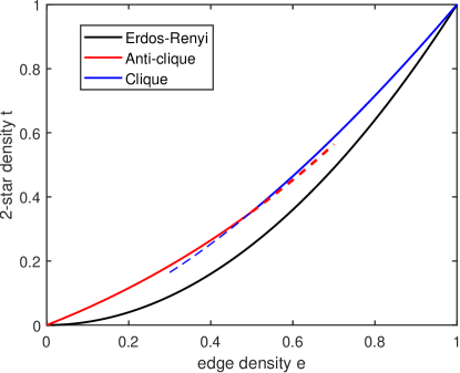
Figure 1. Possible values of $(e,t)$ in the edge-2star model.

Our first result on the edge-2star model concerns the region with edge density close to $1/2$ and 2star density close to the maximum. (See Figure 1.) We show that the open set of graphons with reduced 2star density $\tilde{t}=t-e^{2}$ close to the maximum has two open subsets, one of which we call “clique-like” and the other of which we call “anti-clique-like”, separated by a segment of the line $e=\frac{1}{2}$. (See Figure 2.)

Theorem 1 (Theorems 7,8).

There is an open set in $(e,\tilde{t})$-space containing a segment of the line $e=\frac{1}{2}$ with $\tilde{t}$ just below its maximum of $\frac{\sqrt{2}-1}{4}$, such that

• When $e>\frac{1}{2}$, the entropy-optimizing graphon is unique and clique-like,

• When $e<\frac{1}{2}$, the entropy-optimizing graphon is unique and anti-clique-like, and

• When $e=\frac{1}{2}$ there are two entropy-optimizing graphons, one clique-like and one anti-clique-like.

We thus show that, on each side of a segment of the line $e=1/2$, the optimal graphon is bipodal and unique, with parameters that vary smoothly with $e$ and $\tilde{t}$. This implies that there is a discontinuous phase transition across the line $e=\frac{1}{2}$, with typical graphs being anti-clique-like on one side of the line and clique-like on the other.

The situation is very different when $\tilde{t}$ is small. Let $\zeta=\sqrt{\left(e-\frac{1}{2}\right)^{2}+\tilde{t}}$.

Theorem 2 (Theorem 9).

For sufficiently small $\zeta$, the entropy-maximizing graphon is unique and bipodal, with parameters

(1) $$a = 1-e-2\zeta+O(\zeta^{2}),$$

(2) $$b = 1-e+2\zeta+O(\zeta^{2}),$$

(3) $$d = 1-e+O(\zeta^{2}),$$

(4) $$c = \frac{1}{2}\left(1-\frac{e-\frac{1}{2}}{\zeta}\right)+O(\zeta)$$

that are analytic functions of $(e,\tilde{t})$ everywhere except at the singular point $e=\frac{1}{2}$, $\tilde{t}=0$.

In previous work [7] we had proven that, for $e\neq 1/2$ and $\tilde{t}$ sufficiently small, there is a unique optimal graphon that is bipodal. Theorem 2 bridges the gap between the regions $e<1/2$ and $e>1/2$ and shows that there is a single phase just above the entire Erdős-Rényi curve $\tilde{t}=0$.

Now consider what happens along the line $e=1/2$. When $\tilde{t}$ is small, Theorem 2 implies that there is a unique optimal graphon that is bipodal. Uniqueness implies that the four parameters satisfy $a+b=1$ and $c=d=1/2$. At some point on the line a graphon of this form ceases to be optimal, since Theorem 1 says that, for $e=1/2$ and $\tilde{t}$ sufficiently large, there are two optimal graphons, one clique-like and the other anti-clique-like. At some point in between there must be a point of non-analyticity, where symmetry is broken and the structure of the optimal graphon changes.

Determining the exact nature of this bifurcation point is beyond our current methods, as it is conceivable that the optimal graphon might change discontinuously. Instead, we determine where the symmetric graphon becomes stable against small changes.

Theorem 3 (Theorem 11).

There is a number $\tilde{t}^{*}\approx 0.03727637$ such that

1. For all $\tilde{t}<\tilde{t}^{*}$, there is a bipodal graphon with $b=1-a$, $c=d=1/2$, that is a local maximizer of the entropy among all bipodal graphons with edge density $1/2$ and 2star density $\tilde{t}+\frac{1}{4}$.

2. If $\tilde{t}^{*}<\tilde{t}\leq 0.0625$, then there exist bipodal graphons with $b=1-a$ and $c=d=1/2$, but these graphons are not local maximizers.

3. If $\tilde{t}>0.0625$, then there do not exist bipodal graphons with $b=1-a$ and $c=d=1/2$.

1.2. Background and formalism

To put these results about the edge-2star model in context, and to explain our foundational results, we review some relevant history of research into ensembles of large dense random graphs.

Following the publication by Chatterjee/Varadhan [5] of the LDP of the Erdős-Rényi random graph $G(n,p)$, Chatterjee/Diaconis popularized [3] the use of graphons, with ‘soft’ constraints on the densities of several subgraphs $P_{j}$, to analyze exponential random graph models (ERGMs). The graphon formalism of Lovász and coauthors [1, 2, 9, 10, 11] allows graphs $G$ on any finite number of nodes to be incorporated, as ‘checkerboard graphons’ $g^{G}$, in the space ${\mathcal{W}}$ of their ‘infinite node limits’, graphons; for an in-depth presentation we recommend [12].

The LDP is expressed in terms of probability distributions $\mathcal{P}_{n}$ on ${\mathcal{W}}$ (and the closely connected $\widetilde{\mathcal{P}_{n}}$ on reduced graphons $\widetilde{\mathcal{W}}$), associated with a sequence $p_{n}$ of discrete distributions on the sets $\mathcal{G}_{n}$ of graphs on $n$ nodes. Given their focus on ERGMs, in [3] the constraints on the subgraphs $P_{j}$ were naturally implemented by the choice of exponential distributions for $p_{n}$:

(5) $$p_{n}(G)=e^{n^{2}T({g^{G}})-\psi_{n}},$$

where $\psi_{n}$ is a normalizing constant,

(6) $$T(g)=\sum_{j=1}^{k}\beta_{j}\tau_{j}(g)$$

is a function on graphons, and $\tau_{j}(g)$ is the density of $P_{j}$ in the graphon $g$. The parameters of the model are the $\beta^{\prime}s$, and the constrained graphons for given parameter values are the graphons $g$ that optimize the functional $T(g)+S(g)$, where

(7) $$S(g):=\int_{0}^{1}\!\!\int_{0}^{1}H(g(x,y))dx\,dy\qquad\hbox{ and }H(u):=-\frac{1}{2}(u\ln(u)+(1-u)\ln(1-u)).$$

The quantity $S(g)$, which we call the Shannon entropy of the graphon $g$, is closely related to the LDP rate function $\tilde{I}_{p}(g)$ of [3]. Specifically, $S(g)=\frac{1}{2}\ln(2)-\tilde{I}_{1/2}(g)$.

Both [5] and [3] emphasize the difficulty of accessing/determining nonconstant optimal graphons; the formalism easily leads to Erdős-Rényi optima. (See for instance the open questions section 4.8, in [5].) It was to overcome this tendency that a variant graphon model was introduced in [20, 21] using hard rather than soft constraints on the subgraphs $P_{j}$; the parameters were chosen to be the densities of the $P_{j}$ and the role of the discrete distribution $p_{n}$ on $\mathcal{G}_{n}$ was replaced by a two-step process. Then the appropriately constrained graphons for given values of the parameters are characterized as those $g$, with the given parameter densities, which optimize $I(g)$. (See [6] for a connection to large deviations for $G(n,m)$.)

This modified approach to parametric graphon models achieved the initial goal of [20, 21], the determination of a fully explicit nonconstant and unique optimizer for each constraint on a line in the edge-triangle model. The goal then expanded. In [3] (indeed already in [5]) attention was drawn to singular behavior (‘phase transitions’) that appeared as the model parameters were varied. Our extended goal was to determine a ‘phase’, an open set of parameters, with a unique, optimizing graphon associated to each point, which moreover responds smoothly with variation of the parameters. (Note that Erdős-Rényi graphs are automatically represented by constraint parameters on a curve in parameter space, and from smoothness cannot be contained in a phase.) This took a few years to accomplish but was obtained [8] in a broad class of models: constraints on edges and any one other graph, $P$. Finally, after another few years, we determined [15] a ‘transition’, a pair of phases separated by a transition curve. We emphasize that in these models with hard constraints such transitions represent sharp structural changes in the ‘typical’ large graph as the parameters vary, where typical means all but exponentially few as the node number diverges.

An important lesson learned was that, as in the more general subject of deviations in $G(n,p)$ from which this all stems [5], in analyzing our deviations it is significant whether we are dealing with an upper tail or lower tail; for a model with fixed constraints on the density of edges and one other graph $P$, it is significant whether the density for $P$ is larger or smaller than it is for Erdős-Rényi graphs with the same edge density. (This is a very large subject; for a good overview we recommend [4]. For a particularly relevant connection to this paper see [14], and references therein.) To prove the more detailed results such as phase transitions required focusing on a narrower range of models, edge-triangle for lower tail features and edge-2star for upper tail. In the edge-triangle model we recently determined [16] a ‘symmetric’ phase which could be distinguished by an order parameter, and, in the present paper, in the edge-2star model we determine a discontinuous transition.

1.3. Foundational results

Our goal is to analyze large graphs with hard constraints on the densities of a number of subgraphs, typically the density $e$ of edges and $t_{P}$ of another subgraph $P$. If $P$ has $m$ vertices and $\ell$ edges, with edge $e_{k}$ connecting vertices $s_{k}$ and $f_{k}$, then the density of $P$ associated with a graphon $g$ is given by the functional

(8) $$\tau(g):=\int\prod_{k=1}^{\ell}g(x_{s_{k}},x_{f_{k}})d^{m}x.$$

If we are considering multiple subgraphs $P_{i}$, then we will refer to the density function for $P_{i}$ as $\tau_{i}(g)$ and a typical value of this functional as $t_{i}$.

The key tool for counting finite graphs with subgraph densities in a given range is the LDP of Chatterjee and Varadhan [5]:

Theorem 4.

For any closed set $\tilde{F}\subseteq\widetilde{{\mathcal{W}}}$, and using the notation $|A^{n}|$ for the number of graphs on $n$ nodes whose checkerboard graphons $g^{G}$ lie in $A$, we have

(9) $${\lim\sup}_{n\to\infty}\frac{1}{n^{2}}\ln(|\tilde{F}|)\leq{\sup}_{\tilde{g}\in\tilde{F}}\ S(\tilde{g})$$

and for any open set $\tilde{U}\subseteq\widetilde{{\mathcal{W}}}$,

(10) $${\lim\inf}_{n\to\infty}\frac{1}{n^{2}}\ln(|\tilde{U}|)\geq{\sup}_{\tilde{g}\in\tilde{U}}\ S(\tilde{g}).$$

To apply this theorem to graphs with constraints on subgraphs $P_{1},\ldots,P_{k}$, we merely take $\tilde{F}$ and $\tilde{U}$ to be sets of graphons whose densities $(\tau_{1}(g),\ldots,\tau_{k}(g))$ lie in open and closed subsets of $\mathbb{R}^{k}$. We say that a collection $(t_{1},\ldots,t_{k})$ is achievable if there exists at least one graphon $g$ with $(\tau_{1}(g),\ldots,\tau_{k}(g))=(t_{1},\ldots,t_{k})$.

Next we define the Boltzmann entropy. If we are constraining the densities of $k$ subgraphs $P_{1},\ldots P_{k}$, let $\displaystyle Z^{n,\delta}_{t_{1},\ldots,t_{k}}$ be the number of simple graphs $G$ such that the density of each $P_{i}$ is in the interval $(t_{i}-\delta,t_{i}+\delta)$. Let $\displaystyle B^{n,\delta}_{t_{1},\ldots,t_{k}}={\ln(Z^{n,\delta}_{t_{1},\ldots,t_{k}})}/{n^{2}}$ and consider

(11) $$\lim_{\delta\to 0^{+}}\lim_{n\to\infty}B^{n,\delta}_{t_{1},\ldots,t_{k}}.$$

The double limit exists, defining $B_{t_{1},\ldots,t_{k}}$, and there is a variational characterization of it, proven using the LDP. The following is a generalization of results proven in [20, 21] (first for edges and triangles, then for edges and one other subgraph).

Theorem 5.

For any achievable $k$-tuple $(t_{1},\ldots,t_{k})$, the limit (11) defining $B_{t_{1},\ldots,t_{k}}$ exists and equals $\max S(g)$, where the maximum is over all graphons $g$ with $(\tau_{1}(g),\ldots,\tau_{k}(g))=(t_{1},\ldots,t_{k})$.

The (constrained) graphon $g$ that maximizes $S(g)$ doesn’t just determine the number of large graphs with subgraph densities close to $t_{1},\ldots,t_{k}$. When the optimal graphon is unique, it also determines the form of all but an exponentially small fraction of those graphs. The following theorem states precisely what we mean when we say that a typical large graph with densities $(t_{1},\ldots,t_{k})$ looks like $g_{0}$.

Theorem 6.

Let $(t_{1},\ldots,t_{k})$ be a point in the space of achievable parameter values in a model with $k$ constrained subgraphs, and suppose that there is a unique (reduced) graphon $g_{0}$ that maximizes $S(g)$ subject to the constraint $(\tau_{1}(g),\ldots,\tau_{k}(g))=(t_{1},\ldots,t_{k})$. For any positive constants $\delta$ and $n$, let $\mathcal{G}_{\delta,n}$ be the set of labeled graphs on $n$ vertices with densities $\tau_{i}(g)$ in $(t_{i}-\delta,t_{i}+\delta)$ for each $i$. Then, for any $\epsilon>0$, there exist positive constants $\delta$, $N$ and $K$ such that, for all $n>N$, the fraction of graphs in $\mathcal{G}_{\delta,n}$ that are within $\epsilon$ of $g_{0}$ in the cut metric exceeds $1-e^{-Kn^{2}}$.

Note that if $S(g_{0})=0$, then the number of graphs in $\mathcal{G}_{\delta,n}$ for small $\delta$ grows slower than $e^{Kn^{2}}$. Theorem 6 then implies that, for $\delta$ sufficiently small, all graphs in $\mathcal{G}_{\delta,n}$ are within $\epsilon$ of $g_{0}$.

The organization of this paper is as follows. In Section 2 we review what has been previously proven about the edge-2star model. In Section 3 we consider the situation where the edge density $e$ is close to $1/2$ and the 2star density $t$ is close to its maximum and prove Theorem 1. In Section 4 we study a neighborhood of $(e,\tilde{t})=(1/2,0)$ and prove Theorem 2. In Section 5 we study the stability of the graphons found in Section 4 and prove Theorem 3. Finally, in the Appendix we prove the foundational Theorems 5 and 6.

2. Old results about the edge-2star model

In this section we review some facts about optimal graphons in the edge-2star model. For detailed proofs, see [7].

Let

$$d(x)=\int_{0}^{1}g(x,y)dy$$

be the degree function of the graphon $g$. The 2star density is then

$$t=\int_{0}^{1}d(x)^{2}\,dx.$$

We also define the reduced 2star density

$$\tilde{t}=t-e^{2}=\int_{0}^{1}(d(x)-e)^{2}\,dx.$$

The minimum value of $\tilde{t}$ is obviously zero, and is achieved when $d(x)$ is constant. Among constant-degree graphons with edge density $e$, the entropy maximizer is the (constant) Erdős-Rényi graphon $g(x,y)=e$.

The maximum value of $t$ depends on $e$. When $e>1/2$, the maximum value of $t$ is $e^{3/2}$ and is achieved by a clique. This is a graphon that is 1 on a square $I\times I$, where $I$ is an interval of width $\sqrt{e}$, and is zero everywhere else. When $e<1/2$, however, the maximum value of $t$ is $(1-e)^{3/2}+2e-1$ and is achieved by an anti-clique. This is a graphon that is equal to 0 on a square of side $\sqrt{1-e}$ and is 1 everywhere else. When $e=1/2$, the maximum value of $t$ is $\sqrt{2}/4\approx 0.3535$ and is achieved by either a clique or an anti-clique, in either case with the interval having width $\sqrt{2}/2$.

If we replace a graphon $g$ with $1-g$, then this changes $e$ to $1-e$, but does not change $\tilde{t}$ or the entropy $S$. Applying the symmetry to an optimal graphon for given values $(e,\tilde{t})$ gives an optimal graphon with values $(1-e,\tilde{t})$. The possible values of the edge and 2star densities are more cleanly expressed in terms of $\tilde{t}$ rather than $t$, as in Figure 2.

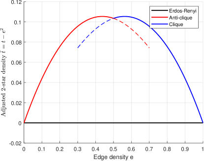
Figure 2. Possible values of $(e,\tilde{t})$ in the edge-2star model.

At a stationary point of the entropy, the degree function $d(x)$ determines the graphon via the equation

(12) $$g(x,y)=\frac{1}{1+\exp(-(\alpha+\beta(d(x)+d(y))))},$$

where $\alpha$ and $\beta$ are Lagrange multipliers, with $dS=\alpha de+\beta dt$ as we vary the graphon in arbitrary ways. By integrating over $y$ we get the self-consistency equation

(13) $$d(x)=\int_{0}^{1}\frac{dy}{1+\exp(-(\alpha+\beta(d(x)+d(y))))}.$$

That is, the only possible values of $d(x)$ are solutions to the equation

(14) $$z=k(z):=\int_{0}^{1}\frac{dy}{1+\exp(-(\alpha+\beta(z+d(y))))}.$$

Both sides of equation (14) are analytic functions of $z$, so there can only be a finite number of solutions. This implies that all graphons that are stationary points of the constrained entropy functional are multipodal.

3. Optimal graphons when $\tilde{t}$ is large

We say that a graphon is clique-like if its degree function is $L^{1}$-close to a step function with values $\sqrt{e}$ and 0, and is anti-clique-like if its degree function is $L^{1}$-close to a step function with values $1-\sqrt{1-e}$ and 1. As we approach the upper boundary, all graphons must be clique-like or anti-clique-like, since otherwise we could take a limit as $t$ approaches the maximum and get a $t$-maximizing graphon that isn’t a clique or an anti-clique. In particular, all of the entropy-maximizing graphons in a neighborhood of $(e,\tilde{t})=\left(\frac{1}{2},\frac{1}{4}(\sqrt{2}-1)\right)$ must be clique-like or anti-clique-like. The two sets are related by the $g\leftrightarrow 1-g$ symmetry, so it is sufficient to study clique-like graphons.

Let $g$ be a clique-like graphon that is a stationary point of the entropy. If we increase the size $c\approx\sqrt{e}$ of the pode(s) with degree function close to $\sqrt{e}$ at the expense of those with degree function close to $0$, then we do not change the set of values achieved by $H(g(x,y))$. We only change the area of the regions where each value is achieved. This means that the change in the entropy (per change in $e$ or $t$) is bounded by a multiple of the existing entropy, which goes to zero as we approach the upper boundary. That is, with this move we must have

(15) $$\alpha\frac{de}{dc}+\beta\frac{dt}{dc}=\frac{dS}{dc}=o(1).$$

It is easy to check that $\frac{dt}{dc}\approx\frac{3}{2}\sqrt{e}\frac{de}{dc}$, so

(16) $$\frac{\alpha}{\beta}=-\frac{3}{2}\sqrt{e}+o(1)$$

Note that $\beta$ is negative, as the entropy decreases as we approach the upper boundary, so $\alpha$ is positive. Both parameters diverge as we approach the upper boundary.

Theorem 7.

There is an open set $U$ in $(e,\tilde{t})$-space containing a segment of the line $e=\frac{1}{2}$ with $\tilde{t}$ just below its maximum of $\frac{\sqrt{2}-1}{4}$, such that

• When $e>\frac{1}{2}$, the entropy-optimizing graphon is clique-like, and

• When $e<\frac{1}{2}$, the entropy-optimizing graphon is anti-clique-like.

Proof.

Thanks to the $g\leftrightarrow 1-g$ symmetry that changes $e$ to $1-e$ and swaps clique-like and anti-clique-like graphons, the second statement is equivalent to the first, so it is sufficient to prove the first. We henceforth assume that $e>1/2$ and that both clique-like and anti-clique-like graphons exist with densities $(e,\tilde{t})$.

Let $S_{c}(e,\tilde{t})$ be the maximum entropy achievable by a clique-like graphon and let $S_{a}(e,\tilde{t})$ be the maximum achievable by an anti-clique-like graphon. Thanks to our $g\leftrightarrow 1-g$ symmetry,

(17) $$S_{c}(e,\tilde{t})=S_{a}(1-e,\tilde{t}),$$

and in particular $S_{c}(\frac{1}{2},\tilde{t})=S_{a}(\frac{1}{2},\tilde{t})$. If we have the optimal clique-like graphon and move along a line of constant $\tilde{t}$, then $dt=2ede$, so the change in entropy is proportional to $(\alpha+2e\beta)de$. By equation (16),

(18) $$\alpha+2e\beta\approx\left(2e-\frac{3}{2}\sqrt{e}\right)\beta\approx\left(1-\frac{3\sqrt{2}}{4}\right)\beta.$$

Since $\beta$ is negative and $3\sqrt{2}/4>1$, this quantity is positive, making $S_{c}(e,\tilde{t})$ an increasing function of $e$. In particular,

(19) $$S_{c}(e,\tilde{t})>S_{c}(1-e,\tilde{t})=S_{a}(e,\tilde{t}).$$

That is, the best clique-like graphon has a higher value of $S$ than the best anti-clique-like graphon, so the best overall graphon is clique-like. ∎

Theorem 8.

On the subset of $U$ where $e\geq 1/2$, the optimal clique-like graphon is unique and bipodal.

Combined with Theorem 7, this says that there is a unique entropy-maximizing graphon when $e>1/2$, and that this optimizing graphon is clique-like and bipodal. By the $g\to 1-g$ symmetry, there is a unique entropy-maximizing graphon when $e<1/2$, and that graphon is anti-clique-like and bipodal. When $e=1/2$, there are exactly two optimizing graphons, both bipodal, one clique-like and one anti-clique-like.

Proof.

First note that optimal graphons must exist for each $(e,\tilde{t})$, thanks to the compactness of the space of reduced graphons and the semi-continuity of the Shannon entropy functional $S(g)$. With that in mind, suppose that $g$ is an optimal clique-like graphon. We will prove properties of $g$ in stages:

1. The degree function $d(x)$ only takes values close to 0, $\frac{1}{2}\sqrt{e}$, or $\sqrt{e}$.

2. The degree function $d(x)$ only takes values close to 0 or $\sqrt{e}$.

3. The degree function $d(x)$ only takes two values, one close to 0 and one close to $\sqrt{e}$. That is, $g$ is bipodal.

4. The parameters that define this bipodal graphon are uniquely determined.

Plugging equation (16) into equations (12 –14) gives

(20) $$g(x,y) = \frac{1}{1+\exp(-\beta(d(x)+d(y)-\frac{3}{2}\sqrt{e}+o(1)))}$$

(21) $$d(x) = \int_{0}^{1}\frac{dy}{1+\exp(-\beta(d(x)+d(y)-\frac{3}{2}\sqrt{e}+o(1)))}$$

(22) $$k(z) = \int_{0}^{1}\frac{dy}{1+\exp(-\beta(z+d(y)-\frac{3}{2}\sqrt{e}+o(1)))}.$$

Since $\beta$ is large, the function $\frac{1}{1+\exp(-\beta(d(x)+d(y)-\frac{3}{2}\sqrt{e}+o(1)))}$ is close to 1 whenever $d(x)+d(y)$ is bigger than $\frac{3}{2}\sqrt{e}$, is close to 0 whenever $d(x)+d(y)$ is smaller than $\frac{3}{2}\sqrt{e}$, and only takes values substantially different from 0 or 1 when $d(x)+d(y)$ is very close to a fixed threshold value that is $\frac{3}{2}\sqrt{e}+o(1)$. Note that $\sqrt{e}\approx\sqrt{2}/2>2/3$, so the threshold is greater than 1. Since the function $d(y)$ is close to 0 on a set of measure approximately $1-\sqrt{e}$ and close to $\sqrt{e}$ on a set of measure approximately $\sqrt{e}$, and only takes on other values on sets of small measure, the function $k(z)$ is approximately a step function, as shown in Figure 3.

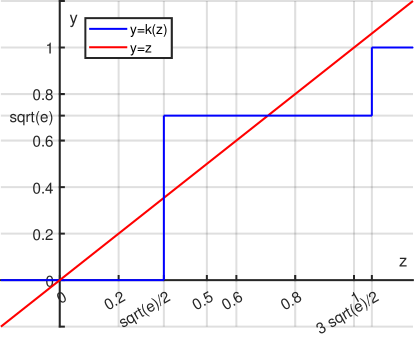
Figure 3. There are only 3 solutions of $k(z)=z$.

Of course the function $k(z)$ isn’t exactly a step function. However, changing the graph of $k(z)$ slightly by having $\beta$ finite and making $L^{1}$-small changes to $d(y)$ can’t create intersection points far from where they already are. The only possible values of $z$ are close to 0, close to $\sqrt{e}/2$ or close to $\sqrt{e}$, as claimed. This completes the first step.

Let $I_{1}$ be the union of all the podes where $d(x)$ is close to $\sqrt{e}$, let $I_{2}$ be the union of all the podes where $d(x)$ is close to $\frac{1}{2}\sqrt{e}$, and let $I_{3}$ be the union of all the podes where $d(x)$ is close to 0. By the definition of clique-like, the measure of $I_{1}$ must be close to $\sqrt{e}$, the measure of $I_{3}$ must be close to $1-\sqrt{e}$ and the measure of $I_{2}$ must be close to 0.

Note that $d(x)+d(y)$ is above the threshold of $\frac{3}{2}\sqrt{e}$ on $I_{1}\times I_{1}$, is close to the threshold on $I_{1}\times I_{2}\cup I_{2}\times I_{1}$, and is below the threshold everywhere else. This implies that $g(x,y)$ is pointwise close to 1 on $I_{1}\times I_{1}$, takes on the average value $1/2$ on $I_{1}\times I_{2}$ (in order for the degree function to be $\frac{1}{2}\sqrt{e}$) and is close to zero everywhere else.

Now consider what happens as we vary the size of $I_{2}$ while keeping $e$ fixed. The entropy associated with the region $I_{1}\times I_{2}\cup I_{2}\times I_{1}$ is linear in the size of $I_{2}$, as is the extent to which $\tilde{t}$ (which is the variance of the degree function) is reduced from the maximum. That is, $\beta$ must be $O(1)$. However, $\beta$ must diverge as $t$ approaches the maximum value, as otherwise the graphon would not approach 0 on $I_{1}\times I_{1}$ and 1 on $I_{3}\times I_{3}$. This contradiction implies that the size of $I_{2}$ is in fact zero, completing the second step.

Next we consider the solutions of $k(z)=z$ near $z=0$ and $z=\sqrt{e}$. Having multiple podes with $d(x)$ close to 0, or multiple podes with $d(x)$ close to $\sqrt{e}$, could smear the vertical part of the step function somewhat, but the portions of the graph near 0 and $\sqrt{e}$ are nearly flat. (If there were any podes with $d(x)$ close to $\sqrt{e}/2$, that would introduce small steps near $z=\sqrt{e}$, insofar as the threshold is $\frac{3}{2}\sqrt{e}$, but we just ruled out the existence of such podes.) Since $k^{\prime}(z)$ is never greater than 1 near $z=0$ or $z=\frac{1}{2}\sqrt{e}$, there can only be one point near 0 and only one point near $\sqrt{e}$ where $k(z)=z$. That is, the graphon must be bipodal, completing the third step.

A bipodal graphon is described by four parameters $(a,b,c,d)$, all between 0 and 1, with

(23) $$g(x,y)=\begin{cases}a&x,y<c\cr b&x,y>c\cr d&x<c<y\hbox{ or }y<c<x\end{cases}$$

Since we are looking for clique-like graphons, we want $a\approx 1$, $b\approx 0$, $c\approx\sqrt{e}$, $d\approx 0$. We compute the gradient of the edge density, 2star density and entropy with respect to $(a,b,c,d)$ and set

(24) $$\nabla S=\alpha\nabla e+\beta\nabla t.$$

Those four equations, plus the constraints on $e$ and $t$, give six equations in six unknowns. The system of equations is non-degenerate and yields a single family of solutions with $a\approx 1$, $b\approx 0$, $c\approx\sqrt{e}$, and $d\approx 0$, namely

(25) $$a = 1-\delta+O(\delta^{2})$$

(26) $$b = O(\delta^{3})$$

(27) $$c = \sqrt{e}+(\frac{3}{2}\sqrt{e}-1)\delta+O(\delta^{2})$$

(28) $$d = \delta+O(\delta^{2}),$$

where $\delta$ is a small parameter. ∎

4. Above Erdős-Rényi

We now turn to the bottom of our parameter space, a neighborhood of the Erdős-Rényi curve $t=e^{2}$, or equivalently $\tilde{t}=0$. In previous work, we identified what happened for $e\neq 1/2$ and $\tilde{t}$ sufficiently small (where “sufficiently small” is $o((e-1/2)^{2})$ as $e\to 1/2$). We showed that, when $e\neq 1/2$, the optimal graphon is bipodal with $c=\frac{\tilde{t}}{4(e-\frac{1}{2})^{2}}+O(\tilde{t}^{2})$ and $d=1-e+O(\tilde{t})$. In particular, the degree function is close to $e$ on the large pode and $1-e$ on the small pode.

In this section we bridge the gap between these two regions, proving that the optimal graphon is unique and bipodal, with parameters that vary smoothly with $e$ and $\tilde{t}$, whenever $\tilde{t}+(e-\frac{1}{2})^{2}$ is small.

The strategy of proof is a variation of a method we used in [16] to determine the optimal graphon in the edge-triangle model below the Erdős-Rényi curve and when $e\approx 1/2$. We begin with an explicit bipodal graphon. Using a power-series expansion of the entropy function $H(u)$, we express the entropy of a graphon in terms of the even moments of $(g(x,y)-\frac{1}{2})$. By examining the first few moments, we show that an optimal graphon has to be close, first in an integral sense and then pointwise, to our model graphon. Finally, we use the consistency equation (14) to show that the optimal graphon is exactly bipodal and unique.

4.1. The ansatz

Let

(29) $$\zeta=\sqrt{\tilde{t}+(e-\frac{1}{2})^{2}},$$

and consider the bipodal graphon $g_{0}$ with

(30) $$a = 1-e-2\zeta,$$

(31) $$b = 1-e+2\zeta,$$

(32) $$d = 1-e,$$

(33) $$c = \frac{1}{2}\left(1-\frac{e-\frac{1}{2}}{\zeta}\right).$$

The degree function is exactly $\frac{1}{2}-\zeta$ on the pode of size $c$ and $\frac{1}{2}+\zeta$ on the pode of size $1-c$.

For fixed $e\neq\frac{1}{2}$, this is the same, to leading order in $\tilde{t}\ll(e-\frac{1}{2})^{2}$, as what was previously proven. When $e=\frac{1}{2}$, this is a symmetric graphon with $c=\frac{1}{2}$ and $b=1-a$. Except at $e-\frac{1}{2}=\tilde{t}=0$, the parameters $(a,b,c,d)$ are analytic functions of $e$ and $\tilde{t}$.

Theorem 9.

For sufficiently small $\zeta$, the entropy-maximizing graphon is unique and is well-approximated by the ansatz graphon $g_{0}$. Specifically, the entropy-maximing graphon has

(34) $$a = 1-e-2\zeta+O(\zeta^{2}),$$

(35) $$b = 1-e+2\zeta+O(\zeta^{2}),$$

(36) $$d = 1-e+O(\zeta^{2}),$$

(37) $$c = \frac{1}{2}\left(1-\frac{e-\frac{1}{2}}{\zeta}\right)+O(\zeta).$$

Furthermore, the exact values of the parameters $a$, $b$, $c$, and $d$ are analytic functions of $(e,\tilde{t})$ everywhere except at the singular point $(\frac{1}{2},0)$.

Corollary 10.

There is an open set in the $(e,\tilde{t})$ plane, whose lower boundary is the entire open line segment $\tilde{t}=0$, $0<e<1$, on which the optimizing graphon is bipodal and unique. On this open set, the parameters $(a,b,c,d)$ are analytic functions of $(e,\tilde{t})$.

That is, there is a single bipodal phase just above $\tilde{t}=0$. This has implications for the edge-triangle model and for all models where we constrain the density of edges and another connected graph $H$ whose vertices all have valence 1 or 2. In [8], we proved results about such models for $e\neq 1/2$ by relating the change in the number of $H$’s to changes in the number of 2stars. A similar approach is promising for $e\approx 1/2$. However, the estimates become delicate as $e\to\frac{1}{2}$, so we postpone that analysis to a future work.

Proof of Theorem 9.

Any graphon $g$ with degree function

(38) $$d(x)=\int_{0}^{1}g(x,y)dy$$

can be uniquely written as

(39) $$g(x,y) = d(x)+d(y)-e+\delta g(x,y)$$

(40) $$= (d(x)-\frac{1}{2})+(d(y)-\frac{1}{2})+(1-e)+\delta g(x,y)$$

(41) $$g(x,y)-\frac{1}{2} = (d(x)-\frac{1}{2})+(d(y)-\frac{1}{2})-(e-\frac{1}{2})+\delta g(x,y),$$

where $\delta g(x,y)$ is a function with zero marginals:

(42) $$\int_{0}^{1}g(x,y)\,dx=\int_{0}^{1}g(x,y)\,dy=0.$$

We will show that $\delta g(x,y)$ is pointwise $O(\zeta^{2})$ and that $d(x)-\frac{1}{2}$ only takes on two values, within $O(\zeta^{2})$ of $\pm\zeta$. This implies that $g$ is bipodal and follows the estimates (34). The analyticity of $(a,b,c,d)$ then follows from the implicit function theorem. The proof follows several steps:

1. Using known properties of the entropy function near Erdős-Rényi to estimate the Lagrange multipliers $\alpha$ and $\beta$ that appear in equations (12–14).

2. Showing that $g$ is at most tripodal and that the degree function is everywhere $\frac{1}{2}+o(1)$. This implies that $g$ is pointwise close to $\frac{1}{2}$.

3. Comparing the entropy of the general graphon $g(x,y)$ of equation (39) to the entropy of the ansatz graphon $g_{0}$. This will show that $\iint\delta g(x,y)^{2}dx\,dy=O(\zeta^{6})$, that $g_{0}$ comes within $O(\zeta^{6})$ of achieving the maximum possible entropy, and that the variance of $(d(x)-\frac{1}{2})^{2}$ is $O(\zeta^{6})$.

4. Since $(d(x)-\frac{1}{2})^{2}$ is almost constant (in an $L^{2}$ sense), and since $\int_{0}^{1}(d(x)-\frac{1}{2})^{2}\,dx=\zeta^{2}$ (exactly), our graphon must either be bipodal with degrees very close to $\frac{1}{2}\pm\zeta$, or must be tripodal with a very small third pode. We rule out the latter possibility.

5. We examine the variational equations on the space of bipodal graphons in a neighborhood of $g_{0}$ and show that there is a unique solution that depends analytically on $(e,\tilde{t})$.

Step 1: The function $H(u)$ admits a convergent power series expansion around $u=\frac{1}{2}$:

(43) $$H(u)=H\left(\frac{1}{2}\right)+\frac{1}{2}\,H^{\prime\prime}\left(\frac{1}{2}\right)\left(u-\frac{1}{2}\right)^{2}+\frac{1}{24}\,H^{\prime\prime\prime\prime}\left(\frac{1}{2}\right)\left(u-\frac{1}{2}\right)^{4}+\cdots.$$

This gives rise to a convergent power series expansion for the entropy of a graphon $g$:

(44) $$S(g)=\sum_{k=0}^{\infty}\frac{\mu_{2k}}{(2k)!}H^{(2k)}\left(\frac{1}{2}\right),$$

where

(45) $$\mu_{2k}=\iint\left(g(x,y)-\frac{1}{2}\right)^{2k}\,dx\,dy.$$

When $\tilde{t}=0$, the maximal entropy is exactly $H(e)$. As we vary $e$, the infinitesimal change in $t$ is $2ede$, so

(46) $$\alpha+2e\beta=H^{\prime}(e)\approx H^{\prime\prime}\left(\frac{1}{2}\right)\left(e-\frac{1}{2}\right).$$

The existence of the ansatz graphon $g_{0}$, with entropy $H(e)+H^{\prime\prime}(\frac{1}{2})\tilde{t}+O(\zeta^{4})$, shows that $\beta$ is no less than $H^{\prime\prime}(\frac{1}{2})+O(\zeta)=-4+O(\zeta)$. However, if $\beta$ were greater than $H^{\prime\prime}(\frac{1}{2})+O(\zeta)$, then there would only be one solution to equation (14), namely $z=k(z)=e$. But that gives $\tilde{t}=0$. When $\tilde{t}>0$, we must have

(47) $$\alpha=-H^{\prime\prime}(e)+O(\zeta),\qquad\beta=H^{\prime\prime}(e)+O(\zeta).$$

Step 2: With these values of $\alpha$ and $\beta$, the line $y=z$ is nearly tangent to $y=k(z)$ at $y=e$. This implies that all solutions to $z=k(z)$ are close to $e$, or equivalently close to $1/2$.

The function $k(z)$ is the convolution of a fixed (scaled) logistic curve. The logistic function $1/(1+\exp(-(\alpha+\beta(z+e))))$ has a negative third derivative near $z=e$. Any small convolution of this function must likewise have a negative third derivative, meaning that its second derivative is decreasing and only passes through zero once near $z=e$. By Rolle’s theorem, this implies that a line can only intersect the graph $y=k(z)$ at most three times near $z=e$. Thus our optimal graphon must be at most tripodal, with degrees close to 1/2. By equation (12), this means that the graphon is pointwise close to 1/2, meaning that $g(x,y)-\frac{1}{2}$ is $o(1)$ as $\zeta\to 0$.

Step 3: We now compute the leading terms in the expansions of $S(g_{0})$ and $S(g)$. For any graphon, let

(48) $$\nu_{k}=\int_{0}^{1}\left(d(x)-\frac{1}{2}\right)^{k}\,dx.$$

Note that the first two moments are determined by $e$ and $\tilde{t}$:

(49) $$\nu_{1}=e-\frac{1}{2}\hbox{ and }\nu_{2}=\zeta^{2}=\tilde{t}+\left(e-\frac{1}{2}\right)^{2}.$$

Higher even moments are bounded from below:

(50) $$\nu_{2k}\geq\nu_{2}^{k},$$

with equality if and only if $\left(d(x)-\frac{1}{2}\right)^{2}$ is constant. In particular, $\nu_{4}-\nu_{2}^{2}$ is the variance of $\left(d(x)-\frac{1}{2}\right)^{2}$.

Let

$$\eta=\left(\iint\delta g(x,y)^{2}\,dx],dy\right)^{1/2}$$

be the $L^{2}$ norm of $\delta g$. For an arbitrary graphon, the first two non-trivial moments are:

(51) $$\mu_{2} = 2\nu_{2}-\left(e-\frac{1}{2}\right)^{2}+\eta^{2}$$

(56) $$\mu_{4} = 2\nu_{4}+6\nu_{2}^{2}-12\left(e-\frac{1}{2}\right)^{2}\nu_{2}+5\left(e-\frac{1}{2}\right)^{4}$$

$$+24\iint\delta g(x,y)\left[(d(x)-\frac{1}{2})^{2}(d(y-\frac{1}{2})-(e-\frac{1}{2})(d(x)-\frac{1}{2})(d(y-\frac{1}{2})\right]dx\,dy$$

$$+12\iint\delta g(x,y)^{2}\left[(d(x)-\frac{1}{2})^{2}-(d(x)-\frac{1}{2})(d(y)-\frac{1}{2})\right]dx\,dy$$

$$+4\iint\delta g(x,y)^{3}\left[2(d(x)-\frac{1}{2})-(e-\frac{1}{2})\right]dx\,dy$$

$$+\iint\delta g(x,y)^{4}dx\,dy+6(e-\frac{1}{2})^{2}\|\delta g\|_{2}^{2}.$$

For the graphon $g_{0}$, this simplifies to

(57) $$\mu_{2} = 2\nu_{2}-\left(e-\frac{1}{2}\right)^{2}$$

(58) $$\mu_{4} = 2\nu_{2}^{2}-12\nu_{2}(e-\frac{1}{2})^{2}+5(e-\frac{1}{2})^{4}$$

(59) $$= 2\zeta^{4}+6(\zeta^{2}-(e-\frac{1}{2})^{2})^{2}-(e-\frac{1}{2})^{4}.$$

Comparing these, we see that there is an $H^{\prime\prime}(1/2)\eta^{2}$ cost in having $\delta g$ nonzero and a $H^{\prime\prime\prime\prime}(1/2)(\nu_{4}-\nu_{2}^{2})/12$ cost in having $(d(x)-\frac{1}{2})^{2}$ not be constant. There are also costs in $\mu_{4}$ from terms proportional to $\delta g^{2}$ or $\delta g^{4}$.

The lowest-order benefits from having $\delta g$ nonzero are terms proportional to

(60) $$\iint\delta g(x,y)\left(d(x)-\frac{1}{2}\right)^{2}\left(d(y)-\frac{1}{2}\right)dx\,dy$$ and

(61) $$\iint\delta g(x,y)(e-\frac{1}{2})\left(d(x)-\frac{1}{2}\right)\left(d(y)-\frac{1}{2}\right)dx\,dy$$

By Cauchy-Schwarz, the first term is $O(\zeta\eta\sqrt{\nu_{4}})$, while the second is $O(\zeta^{3}\eta)$. Since $\nu_{4}$ cannot be much greater than $\nu_{2}^{2}$, the maximum possible benefit is $O(\zeta^{3}\eta)$.

Any benefits from the expansion of $\mu_{6}$ and higher are higher order in $\zeta$, $\eta$, or both, so the total benefit of having $\delta g$ nonzero is $O(\zeta^{3}\eta)$ With a cost proportional to $\eta^{2}$ and benefits that are $O(\zeta^{3}\eta)$, $\eta$ must itself be $O(\zeta^{3})$ and the net benefit of having $\delta g$ nonzero is $O(\zeta^{6})$.

This means that the net cost associated with having $(d(x)-\frac{1}{2})^{2}$ differ from a constant must itself be $O(\zeta^{6})$. There are indeed benefits at higher order, for instance terms proportional to $(e-\frac{1}{2})\nu_{2}\nu_{3}$ that appear in the expansion of $\mu_{6}$, but they are all $O(\zeta^{6})$, so the cost in $\mu_{4}$, proportional to the variance of $(d(x)-\frac{1}{2})^{2}$, must be $O(\zeta^{6})$.

Step 4: We recall some facts about cubic polynomials. Suppose that

(62) $$f(x)=x^{3}+a_{2}x^{2}+a_{1}x+a_{0}$$

has three real roots. The sum of the roots is $-a_{2}$ and the average of the roots is $-a_{2}/3$, which is also the unique point where $f^{\prime\prime}(x)=0$. Now consider the convolution of $f$ with a distribution of degree functions $d(y)$:

(63) $$\tilde{f}(x)=\int_{0}^{1}f(x+d(y))dy.$$

If $\tilde{f}$ has three roots, then the sum of the roots is $-3e-a_{2}$, where $e=\int_{0}^{1}d(y)dy$ ,and the average of the roots is $-e-\frac{a_{2}}{3}$. Furthermore, a simple algebraic calculations shows that

(64) $$\tilde{f}(-e-\frac{a_{2}}{3})=f(-\frac{a_{2}}{3})+\int_{0}^{1}(d(y)-e)^{3}\,dy.$$

Now consider the function

$$\frac{1}{1+\exp(-(\alpha+\beta z)}$$

Near the point of inflection $z=-\alpha/\beta$, this function is approximately cubic, with corrections of order $(z+\frac{\alpha}{\beta})^{5}$. The value of this function at the point of inflection is exactly 1/2. Convolving this function by the degree function $d(y)$ we obtain the function $k(z)$. The solutions to $k(z)$ have average value $\bar{d}=-e-\frac{\alpha}{\beta}$. The value of $k(\bar{d})$ is $\frac{1}{2}+\int_{0}^{1}(d(x)-e)^{3}\,dx$, plus $O((\bar{d}-e)^{5})$ corrections due to $k(z)$ not being exactly cubic.

We have already shown that two of the three roots of $k(z)-z$ are $\frac{1}{2}\pm\zeta+O(\zeta^{2})$. Since $\int_{0}^{1}d(x)^{3}\,dx$ is then $O(\zeta^{3})$, this implies that the average of the three roots is $\frac{1}{2}+O(\zeta^{3})$, which implies that the third root must be $\frac{1}{2}+O(\zeta^{2})$. Let $c_{3}$ be the size of this pode.

We now compute the cost

(65) $$\nu_{4}-\nu_{2}^{2}=\int_{0}^{1}((d(x)-\frac{1}{2})^{2}-\zeta^{2})^{2}\,dx\approx c_{3}\zeta^{4}.$$

The derivative of the entropy with respect to $c_{3}$ has a positive term of order $\zeta^{4}$. Since $d(x)-\frac{1}{2}$ is pointwise $O(\zeta)$, all of the contributions to $\mu_{6}$ and higher have order $\zeta^{6}$ and higher, and cannot overcome this quartic cost. Nor can the cross-terms with $\delta g$, which we have shown to be $O(\zeta^{6})$. Since the derivative of the entropy with respect to $c_{3}$ is positive, the entropy is maximized when $c_{3}=0$. That is, the optimal graphon is bipodal, not tripodal, with the degree functions on the two podes being $\frac{1}{2}\pm\zeta+O(\zeta^{2})$.

Step 5: Bipodal graphons are described by four parameters $(a,b,c,d)$. The edge density, 2star density, and entropy are all analytic functions of $(a,b,c,d)$. Introducing Lagrange multipliers, we obtain four analytic equations in six unknowns:

(66) $$\nabla S=\alpha\nabla e+\beta\nabla t$$

This gives a 2-dimensional analytic variety of solutions. To see that $(a,b,c,d)$ are analytic functions of $e$ and $t$, we need only check that the tangent space does not degenerate. That is, we must check that on this family of solutions, the edge and triangle densities can be varied independently to first order.

However, that is easy. This property obviously holds for the ansatz graphon (30), except at the singularity $\zeta=0$ (where the derivative of $\zeta$ with respect to $\tilde{t}$ diverges). $\partial d/\partial e=-1$, while $\partial d/\partial\tilde{t}=0$. However, the partial derivatives of $a$, $b$ and $c$ with respect to $\tilde{t}$ are nonzero, showing that $\partial_{e}(a,b,c,d)$ and $\partial_{\tilde{t}}(a,b,c,d)$ are linearly independent vectors. In particular,

(67) $$\frac{\partial a}{\partial e}\frac{\partial d}{\partial\tilde{t}}-\frac{\partial d}{\partial e}\frac{\partial a}{\partial\tilde{t}}=\frac{1}{\zeta}.$$

The difference between the true graphon and the ansatz is small, in particular being $O(\zeta^{2})$ for $a$ and $d$, with the derivatives of these terms with respect to $\zeta$ being $O(\zeta)$. Since

(68) $$\frac{\partial\zeta}{\partial e}=\frac{e-\frac{1}{2}}{\zeta}=O(1)\hbox{ and }\frac{\partial\zeta}{\partial\tilde{t}}=\frac{1}{2\zeta},$$

these terms can only change $\partial_{e}(a)$ and $\partial_{e}(d)$ by $O(\zeta)$ and $\partial_{\tilde{t}}(a)$ and $\partial_{\tilde{t}}d$ by $O(1)$, resulting in an $O(1)$ change in $\partial_{e}a\partial_{\tilde{t}}d-\partial_{e}d\partial_{\tilde{t}}a$, which remains nonzero for small $\zeta$.

∎

5. Bifurcation point(s)

We now turn our attention to the line $e=\frac{1}{2}$. When $\tilde{t}$ is close to $\left(\frac{\sqrt{2}-1}{4}\right)$, there are two optimal graphons, one clique-like and the other anti-clique-like. When $\tilde{t}$ is close to 0, there is a unique optimal graphon, which must be symmetric under $g\leftrightarrow 1-g$. That is, it must be bipodal with $c=d=1/2$ and $b=1-a$. Somewhere between these regions, there must be a bifurcation point $(\frac{1}{2},\tilde{t}^{*})$, where the system transitions from having a unique optimal maximizer to having multiple inequivalent maximizers. In principle there might be multiple critical points; we are guaranteed to have at least one.

We are not prepared to investigate a hypothetical point where a graphon that is far from symmetric has a Shannon entropy that matches and then exceeds the entropy of a symmetric graphon. However, we can answer a simpler question: At what value of $\tilde{t}$ does the bipodal graphon with $a=1-b$ and $c=d=1/2$ stop being a local maximizer of the entropy within the 4-dimensional space of bipodal graphons?

Theorem 11.

There is a critical value $\tilde{t}^{*}\approx 0.03727637$ such that

1. For all $\tilde{t}<\tilde{t}^{*}$, there is a bipodal graphon with $b=1-a$, $c=d=1/2$, that is a local maximizer of the entropy among all bipodal graphons with edge density $1/2$ and 2star density $\tilde{t}+\frac{1}{4}$.

2. If $\tilde{t}^{*}<\tilde{t}\leq 0.0625$, then there exist bipodal graphons with $b=1-a$ and $c=d=1/2$, but these graphons are not local maximizers.

3. If $\tilde{t}>0.0625$, then there do not exist bipodal graphons with $b=1-a$ and $c=d=1/2$.

Proof.

Every bipodal graphon can be expressed as a linear combination of a constant graphon, the function $v(x)+v(y)$, and the function $v(x)v(y)$, where

(69) $$v(x)=\begin{cases}\sqrt{\frac{1-c}{c}}&x<c,\cr-\sqrt{\frac{c}{1-c}}&x>c,\end{cases}$$

for some constant $c$. For any fixed value of $c$, we can adjust the coefficient of $v(x)v(y)$ to maximize the Shannon entropy. This gives us entropy as a function of $c$. By doing a power series expansion around $c=1/2$, we determine whether the symmetric graphon is a local maximum or a local minimum of the entropy.

We therefore consider graphons with $c=\frac{1}{2}+\delta$ and

(70) $$g(x,y)=\frac{1}{2}+\mu[v(x)+v(y)]+\nu\delta v(x)v(y),$$

We put an explicit factor of $\delta$ in the coefficient of $v(x)v(y)$ in order to make $\nu$ an even function of $\delta$. Since we only care about the entropy to order $\delta^{2}$, the dependence of $\nu$ on $\delta$ will not matter. The degree function is then $d(x)=\frac{1}{2}+\mu v(x)$, whose variance is $\mu^{2}$, so $\mu=\sqrt{\tilde{t}}$.

Our symmetric graphons have $a=\frac{1}{2}+2\mu$, $b=\frac{1}{2}-2\mu$, and $c=d=\frac{1}{2}$. Since $a$ and $b$ must be between 0 and 1, $|\mu|$ cannot be greater than $\frac{1}{2}$. These symmetric graphons are only defined when $\tilde{t}\leq\frac{1}{16}=0.0625$.

For general (not necessarily symmetric) bipodal graphons, the four parameters $(a,b,c,d)$ are

(71) $$a = \frac{1}{2}+2\mu\sqrt{\frac{1-c}{c}}+\nu\delta\frac{1-c}{c}$$

(72) $$= \frac{1}{2}+2\mu+(\nu-4\mu)\delta+4(\mu-\nu)\delta^{2}+O(\delta^{3})$$

(73) $$b = \frac{1}{2}-2\mu\sqrt{\frac{c}{1-c}}+\nu\delta\frac{c}{1-c}$$

(74) $$= \frac{1}{2}-2\mu+\delta(\nu-4\mu)+4\delta^{2}(\nu-\mu)+O(\delta^{3})$$

(75) $$c = \frac{1}{2}+\delta$$

(76) $$d = \frac{1}{2}+\mu\left(\sqrt{\frac{1-c}{c}}-\sqrt{\frac{c}{1-c}}\right)-\nu\delta$$

(77) $$= \frac{1}{2}-(4\mu+\nu)\delta+O(\delta^{3}).$$

We expand the values of $H(a)$, $H(b)$ and $H(d)$ in power series, using the facts that
$H^{\prime}(\frac{1}{2}-2\mu)=-H^{\prime}(\frac{1}{2}+2\mu)$ and $H^{\prime\prime}(\frac{1}{2}-2\mu)=H^{\prime\prime}(\frac{1}{2}+2\mu)$.

(79) $$H(a) = H\left(\frac{1}{2}+2\mu\right)+H^{\prime}\left(\frac{1}{2}+2\mu\right)\left[(\nu-4\mu)\delta+4(\mu-\nu)\delta^{2}\right]$$

$$+\frac{1}{2}H^{\prime\prime}\left(\frac{1}{2}+2\mu\right)(\nu-4\mu)^{2}\delta^{2}+O(\delta^{3}),$$

(81) $$H(b) = H\left(\frac{1}{2}+2\mu\right)+H^{\prime}\left(\frac{1}{2}+2\mu\right)\left[(4\mu-\nu)\delta+4(\mu-\nu)\delta^{2}\right]$$

$$+\frac{1}{2}H^{\prime\prime}\left(\frac{1}{2}+2\mu\right)(\nu-4\mu)^{2}\delta^{2}+O(\delta^{3}),$$

(82) $$H(d) = H\left(\frac{1}{2}\right)+\frac{1}{2}H^{\prime\prime}\left(\frac{1}{2}\right)(\nu+4\mu)^{2}\delta^{2}+O(\delta^{3}).$$

The Shannon entropy of a bipodal graphon is

(84) $$S(g) = c^{2}H(a)+(1-c)^{2}H(b)+2c(1-c)H(d)$$

(85) $$= \frac{1}{4}[H(a)+H(b)+2H(d)]+\delta[H(a)-H(b)]+\delta^{2}[H(a)+H(b)-2H(d)].$$

Plugging in our previously computed values of $H(a)$, $H(b)$ and $H(d)$ gives

(88) $$S(g) = \frac{1}{2}\left(H(\frac{1}{2}+2\mu)+H(\frac{1}{2})\right)-6\delta^{2}\mu H^{\prime}(\frac{1}{2}+2\mu)$$

$$+\frac{1}{4}\delta^{2}\left[(\nu-4\mu)^{2}H^{\prime\prime}(\frac{1}{2}+2\mu)+(\nu+4\mu)^{2}H^{\prime\prime}(\frac{1}{2})\right]$$

$$+2\delta^{2}\left(H(\frac{1}{2}+2\mu)-H(\frac{1}{2})\right)+O(\delta^{3}).$$

That is, the change in the entropy from the symmetric graphon with $\delta=0$ is proportional to $\delta^{2}$ (plus higher-order terms). To leading order, the change in entropy is quadratic in $\nu$. This quadratic function is maximized when

(89) $$\nu=4\mu\frac{H^{\prime\prime}(\frac{1}{2}+2\mu)-H^{\prime\prime}(\frac{1}{2})}{H^{\prime\prime}(\frac{1}{2}+2\mu)+H^{\prime\prime}(\frac{1}{2})}.$$

Next we compute $H$, $H^{\prime}$ and $H^{\prime\prime}$ at $\frac{1}{2}$ and $\frac{1}{2}+2\mu$:

(90) $$H(\frac{1}{2})=\frac{1}{2}\ln(2) H(\frac{1}{2}+2\mu)=-\frac{1}{2}\left((\frac{1}{2}+2\mu)\ln(\frac{1}{2}+2\mu)+(\frac{1}{2}-2\mu)\ln(\frac{1}{2}-2\mu)\right)$$

(91) $$H^{\prime}(\frac{1}{2})=0 H^{\prime}(\frac{1}{2}+2\mu)=\frac{1}{2}(\ln(\frac{1}{2}-2\mu)-\ln(\frac{1}{2}+2\mu))$$

(92) $$H^{\prime\prime}(\frac{1}{2})=-2 H^{\prime\prime}(\frac{1}{2}+2\mu)=\frac{-2}{1-16\mu^{2}}$$

The combinations that appear in equation (88) are:

(93) $$H^{\prime\prime}(\frac{1}{2}+2\mu)-H^{\prime\prime}(\frac{1}{2}) =\displaystyle{-2\left(\frac{1}{1-16\mu^{2}}-1\right)} =-2\left(\frac{16\mu^{2}}{1-16\mu^{2}}\right)$$

(94) $$H^{\prime\prime}(\frac{1}{2}+2\mu)+H^{\prime\prime}(\frac{1}{2}) =\displaystyle{-2\left(\frac{1}{1-16\mu^{2}}+1\right)} =-2\left(\frac{2-16\mu^{2}}{1-16\mu^{2}}\right)$$

(95) $$\nu =\displaystyle{4\mu\left(\frac{16\mu^{2}}{2-16\mu^{2}}\right)} =4\mu\left(\frac{8\mu^{2}}{1-8\mu^{2}}\right)$$

(96) $$\nu+4\mu =\displaystyle{4\mu\left(\frac{8\mu^{2}}{1-8\mu^{2}}+1\right)} =\frac{4\mu}{1-8\mu^{2}}$$

(97) $$\nu-4\mu =\displaystyle{4\mu\left(\frac{8\mu^{2}}{1-8\mu^{2}}-1\right)} =4\mu\left(\frac{16\mu^{2}-1}{1-8\mu^{2}}\right).$$

Combining, we have that

(99) $$\frac{\Delta S}{\delta^{2}} = 3\mu\ln\left(\frac{\frac{1}{2}+2\mu}{\frac{1}{2}-2\mu}\right)-\frac{2}{1-16\mu^{2}}\frac{16\mu^{2}(16\mu^{2}-1)^{2}}{4(1-8\mu^{2})^{2}}$$

$$-\frac{2}{4}\frac{16\mu^{2}}{(1-8\mu^{2})^{2}}-\left((\frac{1}{2}+2\mu)\ln(\frac{1}{2}+2\mu)+(\frac{1}{2}-2\mu)\ln(\frac{1}{2}2\mu)+\ln(2)\right)+O(\delta),$$

where the first term is $-6\mu H^{\prime}(\frac{1}{2}+2\mu)$, the second is $\frac{1}{4}(\nu-4\mu)^{2}H^{\prime\prime}(\frac{1}{2}+2\mu)$, the third is $\frac{1}{4}(\nu+4\mu)^{2}H^{\prime\prime}(\frac{1}{2})$, and the last is $2(H(\frac{1}{2}+2\mu)-H(\frac{1}{2}))$. The logarithmic terms simplify to

$$\mu\ln(1+4\mu)-\mu\ln(1-4\mu)-\frac{1}{2}\ln(1-16\mu^{2}),$$

while the algebraic terms simplify to

$$\frac{-16\mu^{2}}{1-8\mu^{2}}.$$

The total is negative when $\mu$ is small, going as $-64\mu^{4}/3$, but turns positive for larger values of $\mu$, diverging logarithmically as $\mu$ approaches 1/4. The crossover point is at

(100) $$\mu^{*}\approx 0.1930708944,\qquad\tilde{t}^{*}\approx 0.0372763703.$$

∎

Appendix

We include here proofs of two key steps in the project which began with [20]; the existence of the Boltzmann entropy, Theorem 5 (proven is less generality in [20, 21]), and the connection with large finite graphs, Theorem 6.

Proof of Theorem 5.

We first prove that $B_{t_{1},\ldots,t_{k}}$ is well-defined. A priori we only know that $\liminf\ln(Z_{t_{1},\ldots,t_{k}}^{n,\delta})/n^{2}$ and $\limsup\ln(Z_{t_{1},\ldots,t_{k}}^{n,\delta})/n^{2}$ exist as ${n\to\infty}$. However, we will show that they both approach $\max S(g)$ as $\delta\to 0^{+}$.

We need to define a few sets. Let $U_{\delta}$ be the set of graphons $g$ with each $\tau_{i}(g)$ strictly within $\delta$ of $t_{i}$, i.e. the preimage of an open $k$-cube of side $2\delta$ in $t$-space, let $F_{\delta}$ be the preimage of the closed $k$-cube. and let $\tilde{U}_{\delta}^{n}$ and $\tilde{F}_{\delta}^{n}$ be the corresponding sets in $\widetilde{\mathcal{W}}$. Let $|U_{\delta}^{n}|$ and $|F_{\delta}^{n}|$ denote the number of graphs with $n$ vertices whose checkerboard graphons lie in $U_{\delta}$ or $F_{\delta}$. By the large deviations principle, Theorem 4,

(101) $$\limsup_{n\to\infty}\frac{\ln|F_{\delta}^{n}|}{n^{2}}\leq\sup_{\tilde{g}\in\tilde{F}_{\delta}}S(\tilde{g}),$$

which also equals $\sup_{g\in F_{\delta}}S(g)$, and

(102) $$\liminf_{n\to\infty}\frac{\ln|U_{\delta}^{n}|}{n^{2}}\geq\sup_{\tilde{g}\in\tilde{U}_{\delta}}S(\tilde{g}),$$

which also equals $\sup_{g\in U_{\delta}}S(g)$. This yields a chain of inequalities

(103) $$\sup_{U_{\delta}}S(g)\leq\liminf\frac{\ln|U^{n}_{\delta}|}{n^{2}}\leq\limsup\frac{\ln|U^{n}_{\delta}|}{n^{2}}\leq\limsup\frac{\ln|F_{\delta}^{n}|}{n^{2}}\leq\sup_{F_{\delta}}S(g)\leq\sup_{U_{\delta+\delta^{2}}}S(g).$$

As $\delta\to 0^{+}$, the limits of $\sup_{U_{\delta}}S(g)$ and $\sup_{U_{\delta+\delta^{2}}}S(g)$ are the same, and everything in between is trapped.

So far we have proven that $\displaystyle B_{t_{1},\ldots,t_{k}}$ exists and equals

(104) $$\lim_{\delta\to 0^{+}}\sup_{g\in U_{\delta}}S(g).$$

This limit is manifestly at least as big as $\max S(g)$, the maximum value of $S(g)$ among graphons with each $\tau_{i}$ exactly equal to $t_{i}$. To see that is cannot be greater, imagine a sequence of graphons $g_{j}$ with each $\tau_{i}(g_{k})$ converging to $t_{i}$, and with $S(g)$ greater than $\max S(g)+\epsilon$. By the compactness of $\widetilde{\mathcal{W}}$, there is a subsequence whose classes in $\widetilde{\mathcal{W}}$ converge to that of a graphon $g_{\infty}$. The densities $\tau_{i}$ are continuous in the cut metric, so $\tau_{i}(g_{\infty})=t_{i}$. The entropy functional is upper-semicontinuous [5], so $S(g_{\infty})\geq\max S(g)+\epsilon$, which contradicts the definition of $\max S(g)$.

∎

Proof of Theorem 6.

Let $U_{\epsilon}$ denote the open set in $\widetilde{\mathcal{W}}$ of graphons whose cut distance from $g_{0}$ is strictly less than $\epsilon$, and let $\bar{U}_{\epsilon}$ be those graphons of distance $\epsilon$ or less. The complements $U_{\epsilon}^{c}$ (resp. $\bar{U}_{\epsilon}^{c}$) are then closed (resp. open) sets of graphons whose distance from $g_{0}$ is greater than or equal to $\epsilon$ (resp. strictly greater than $\epsilon$). Let $V_{\delta}$ (resp. $\bar{V}_{\delta}$) denote the set of all graphons $g$ with densities $\tau_{i}(g)$ in $(t_{i}-\delta,i_{i}+\delta)$ (resp. $[t_{i}-\delta,t_{i}+\delta]$) for each $i$.

If $V_{\delta}\cap\bar{U}_{\epsilon}^{c}$ is empty for any $\delta$, then all checkerboard graphons in $V_{\delta}$ are close to $g_{0}$ and there is nothing left to prove. Otherwise, let $S_{0}=S(g_{0})$. Let $S_{3,\delta,\epsilon}$ be the supremum of $S(g)$ on $V_{\delta}\cap\bar{U}_{\epsilon}^{c}$. For fixed $\epsilon$, let $S_{3}=\lim_{\delta\to 0}S_{3,\delta,\epsilon}$.

The proof proceeds in five steps:

1. For any fixed $\epsilon$, showing that $S_{3}<S_{0}$.

2. Picking $K<S_{0}-S_{3}$ and numbers $S_{1}$ and $S_{2}$, such that $S_{0}>S_{1}>S_{2}>S_{3}$ and $S_{1}=S_{2}+K$.

3. Showing that, for any $\delta$, the number of graphs in $\mathcal{G}_{\delta,n}$ is eventually greater than $\exp(S_{1}n^{2})$.

4. Showing that, for $\delta$ sufficiently small, the number of graphs in $\mathcal{G}_{\delta,n}\cap U_{\epsilon}^{c}$ is eventually smaller than $\exp(S_{2}n^{2})$.

5. Concluding that, for $\delta$ sufficiently small and $n$ larger than a number that depends only on $\delta$ and $\epsilon$, the number of graphs in $\mathcal{G}_{\delta,n}\cap U_{\epsilon}^{c}$ divided by the number of graphs in $\mathcal{G}_{\delta,n}$ is less than $\exp(-Kn^{2})$.

Step 1: Suppose that $S_{3}\geq S_{0}$. Then there would exist a sequence of graphons $g_{1},g_{2},\ldots$ in $U_{\epsilon}^{c}$, with densities approaching $(t_{1},\ldots,t_{k})$, with $\limsup S(g_{j})\geq S_{0}$. As in the proof of Theorem 5, we use the compactness of $\widetilde{\mathcal{W}}$, the continuity of $\tau_{i}$, and the semi-continuity of $S$ to construct a subsequential limit $g_{\infty}\in\bar{U}_{\epsilon}^{c}$ with densities equal to $(t_{1},\ldots,t_{k})$ and with $S(g_{\infty})\geq S_{0}$. That contradicts the uniqueness of $g_{0}$, so we conclude that $S_{3}<S_{0}$.

Note that $S_{3}$ cannot be negative, as the functional $S(g)$ is positive semi-definite. So what happens when $S_{0}=0$? In that case, $V_{\delta}\cap\bar{U}_{\epsilon}^{c}$ must be empty when $\delta$ is small.

Step 2: Take $K=(S_{0}-S_{3})/3$, $S_{1}=S_{0}-K$ and $S_{2}=S_{0}-2K$.

Step 3: For any $\delta>0$, the supremum of $S(g)$ over $V_{\delta}$ is at least $S_{0}$, and so is strictly greater than $S_{1}$. Since $V_{\delta}$ is an open set,

(105) $$\liminf_{n\to\infty}\frac{1}{n^{2}}\ln(\#{\mathcal{G}}_{n,\delta})\geq S_{0}>S_{1},$$

so for all sufficiently large values of $n$, $\#\mathcal{G}_{n,\delta}>\exp(S_{1}n^{2})$.

Step 4: Since $\lim_{\delta\to 0}S_{3,\delta,\epsilon}=S_{3}<S_{2}$, there exists a nonzero value of $\delta$ for which $S_{3,\delta+\delta^{2},\epsilon}<S_{2}$. The number of graphs in $V_{\delta}\cap U_{\epsilon}^{c}$ is bounded by the number of graphs in the closed set $\bar{V}_{\delta}\cap U_{\epsilon}^{c}$ and the entropy $S(g)$ on $\bar{V}_{\delta}\cap U_{\epsilon}^{c}$ is bounded by $S_{3,\delta+\delta^{2},\epsilon}<S_{2}$. By the first half of Theorem 4,

(106) $$\limsup_{n\to\infty}\frac{1}{n^{2}}\ln(\#(\bar{V}_{\delta}\cap U_{\epsilon}^{c}))<S_{2},$$

so the smaller quantity $\#(V_{\delta}\cap U_{\epsilon}^{c})$ grows strictly slower than $\exp(n^{2}S_{2})$, and in particular is eventually bounded by $\exp(n^{2}S_{2})$.

Step 5: Now we consider the order of operations. Given $\epsilon$, we first compute $S_{3}$ and define $k$, $S_{1}$ and $S_{2}$. We then pick a $\delta$ such that the size of $V_{\delta}\cap U_{\epsilon}^{c}$ is bounded by $\exp(n^{2}S_{2})$ for all sufficiently large $n$. The phrase “sufficiently large” means that there is a number $N_{1}$, depending on $\delta$ and $\epsilon$, such that the bound applies for all $n>N_{1}$. Meanwhile, the number of graphs in $\mathcal{G}_{n,\delta}$ is at least $\exp(n^{2}S_{1})$ for all $n$ greater than another constant $N_{2}$. Pick $N=\max(N_{1},N_{2})$.

The upshot is that for this value of $\delta$, and for all $n>N$,

$$\frac{\#(\mathcal{G}_{n,\delta}\cap U_{\epsilon}^{c})}{\#(\mathcal{G}_{n,\delta})}\leq\frac{\exp(n^{2}S_{2})}{\exp(n^{2}S_{1})}=\exp(-Kn^{2}).$$

∎

References

- [1] C. Borgs, J. Chayes and L. Lovász, Moments of two-variable functions and the uniqueness of graph limits, Geom. Funct. Anal. 19 (2010) 1597-1619.
- [2] C. Borgs, J. Chayes, L. Lovász, V.T. Sós and K. Vesztergombi, Convergent graph sequences I: subgraph frequencies, metric properties, and testing, Adv. Math. 219 (2008) 1801-1851.
- [3] S. Chatterjee and P. Diaconis, Estimating and understanding exponential random graph models, Ann. Statist. 41 (2013) 2428-2461.
- [4] S. Chatterjee, Large Deviations for Random Graphs. (Lecture notes for the 2015 Saint-Flour Summer School.) Springer Lecture Notes in Mathematics. Springer, Berlin-Heidelberg, 2017.
- [5] S. Chatterjee and S. R. S. Varadhan, The large deviation principle for the Erdős-Rényi random graph, Eur. J. Comb., 32 (2011) 1000-1017.
- [6] A. Dembo and E. Lubetzky, A large deviation principle for the Erdős-Rényi uniform random graph, Electron. Commun. Probab. 23 (2018) 1-13.
- [7] R. Kenyon, C. Radin, K. Ren, and L. Sadun, Multipodal structures and phase transitions in large constrained graphs, J. Stat. Phys. 168(2017) 233-258.
- [8] R. Kenyon, C. Radin, K. Ren and L. Sadun, Bipodal structure in oversaturated random graphs, Int. Math. Res. Notices 2018(2016) 1009-1044.
- [9] L. Lovász and B. Szegedy, Limits of dense graph sequences, J. Combin. Theory Ser. B 98 (2006) 933-957.
- [10] L. Lovász and B. Szegedy, Szemerédi’s lemma for the analyst, GAFA 17 (2007) 252-270.
- [11] L. Lovász and B. Szegedy, Finitely forcible graphons, J. Combin. Theory Ser. B 101 (2011) 269-301.
- [12] L. Lovász, Large Networks and Graph Limits, American Mathematical Society, Providence, 2012.
- [13] J. Neeman, C. Radin and L. Sadun, Phase transitions in finite random networks, J Stat Phys 181 (2020) 305-328.
- [14] J. Neeman, C. Radin and L. Sadun, Moderate deviations in cycle count, Random Struct. Algorithms (2023), 1-42, https://doi.org/10.1002/rsa.21147.
- [15] J. Neeman, C. Radin and L. Sadun, Typical large graphs with given edge and triangle densities, Probab. Theory Relat. Fields (2023), https://doi.org/10.1007/s00440-023-01187-8.
- [16] J. Neeman, C. Radin and L. Sadun, Existence of a symmetric bipodal phase in the edge-triangle model, arxiv:2211.10498 (2022).
- [17] C. Radin, K. Ren and L. Sadun, The asymptotics of large constrained graphs, J. Phys. A: Math. Theor. 47 (2014) 175001.
- [18] C. Radin, K. Ren and L. Sadun, A symmetry breaking transition in the edge/triangle network model, Ann. Inst. H. Poincaré D 5 (2018) 251-286.
- [19] C. Radin, K. Ren and L. Sadun, Surface effects in dense random graphs with sharp edge constraint, arXiv:1709.01036v2 (2017)
- [20] C. Radin and L. Sadun, Phase transitions in a complex network, J. Phys. A: Math. Theor. 46 (2013) 305002.
- [21] C. Radin and L. Sadun, Singularities in the entropy of asymptotically large simple graphs, J. Stat. Phys. 158 (2015) 853-865.