Mixture Quantiles Estimated by Constrained Linear Regression

Abstract

The paper considers the problem of modeling a univariate random variable. Main contributions: (i) Suggested a new family of distributions with quantile defined by a linear combination of some basis quantiles. This family of distributions has a high shape flexibility and covers commonly used distributions. (ii) Proposed an efficient estimation method by constrained linear regression (linearity with respect to the parameters). Various types of constraints and regularizations are readily available to reduce model flexibility and improve out-of-sample performance for small datasets . (iii) Proved that the estimator is asymptotically a minimum Wasserstein distance estimator and is asymptotically normal. The estimation method can also be viewed as the best fit in quantile-quantile plot. (iv) Case study demonstrated numerical efficiency of the approach (estimated distribution of historical drawdowns of SP500 Index).

1 Introduction

Building a model for univariate distribution involves a trade-off between interpretability, flexibility and tractability. This paper studies a family of distributions that is sufficiently flexible to accommodate most distributions considered in practice, while being straightforward to interpret and estimate.

The suggested family of distributions is similar to the mixture of probability densities constructed by a weighted sum of basis density functions (i.e., cumulative probability function (CDF) is a weighted sum of the basis CDFs). We consider a new family of distributions with quantile (inverse CDF) defined by a weighted sum of some basis quantiles. The idea of quantile aggregation dates back to Vincent (1912). The reader is referred to Ratcliff (1979) for a detailed review and further development. Their motivation is to estimate the population distribution by averaging some known distributions obtained from individuals with equal weights, while we aim to approximate quantiles with a linear combination of basis quantiles. Various types of basis quantile functions have been earlier considered: orthogonal polynomials (Sillitto, 1969), quantiles of normal and Cauchy distribution mixed with linear and quadratic terms (Karvanen, 2006), and quantile of modified logistic distribution (Keelin and Powley, 2011).

Earlier considered approaches are limited in the choice of basis functions and do not guarantee nondecreasingness of the resultant quantile function. Our approach addresses these two issues. The type and number of basis functions in the weighed sum are arbitrary, as long as they are valid quantile functions. We propose to use quantiles of common distributions such as normal and exponential, especially when prior knowledge on the shape of the distribution is available. For more complicated cases, such as multimodal distributions, we can use, for example, the monotone I-spline basis (Ramsay, 1988). Moreover, Papp (2011), Papp and Alizadeh (2014) show that piecewise I-spline with non-negative coefficients can approximate any bounded continuous nondecreasing function. Quantiles of known distributions and the I-spline basis are both continuous and nondecreasing. Therefore, the nondecreasingness of the estimated function is guaranteed by nonnegativity of the weights (sum of nondecreasing functions with non-negative weights is nondecreasing). While Gaussian mixture densities is considered a parametric model, the mixture splines (estimating quantile) is considered a nonparametric model. However, the mixture of splines still has a simple closed-form expression and great flexibility. Monte Carlo simulation can be easily conducted by inverse transform sampling.

To fit the model, we propose to minimize the distance between the sample quantile function and the model at sample probabilities (confidence levels). The distance is determined by the type of error function we choose. We formulate the estimation problem as a constrained linear regression. This approach differs from existing ones. The minimum quantile distance estimation (LaRiccia, 1982; Millar, 1984; Gilchrist, 2007) minimizes the difference between the sample quantile function and the model. Such approach is also widely studied in the literature of minimum Wasserstein distance (Kantorovich–Rubinstein distance) estimator (Bassetti and Regazzini, 2006; Bassetti et al., 2006; Bernton et al., 2019). However, the difference is an integral in the unit interval rather than at sample probabilities. Maximum likelihood estimation (MLE) is inconvenient to use for our model since it requires the derivative of the inverse of sum of quantile functions. Moreover, the optimization problems of mentioned approaches are nonconvex. In contrast, our formulation of linear regression with linear constraints is a convex optimization problem allowing for efficient computation with powerful convex programming solvers. One more method having efficient optimization, Lariccia and Wehrly (1985), uses only a fixed number of quantiles. Moment fitting and the analogous L-moment fitting (Hosking, 1990; Karvanen, 2006) requires calculating unstable high-order moments of the data. We show that L-moment fitting can be incorporated into our framework as a linear constraint. The quantile regression approach in Peng and Uryasev (2023) considers a different objective function which is equivalent to the sum of continuous ranked probability score (Matheson and Winkler, 1976). If there is only one basis function in the model, our proposed estimation method reduces to estimating the location and scale parameters of a distribution by weighted least squares regression (Ogawa, 1951; Lloyd, 1952). Using a similar method, Kratz and Resnick (1996) estimates the tail index of Pareto distribution with logarithm-transformed data.

We studied asymptotic properties of the estimator and demonstrated that the estimator is asymptotically minimum $q$-Wasserstein (Kantorovich–Rubinstein) distance estimator, when the error function is $L_{q}$ norm. This is proved by viewing the objective function of the optimization as a Monte Carlo integration of the difference between two quantile functions. Different from Bassetti and Regazzini (2006); Bassetti et al. (2006); Bernton et al. (2019), the objective function in our approach is not the $q$-Wasserstein distance between the empirical quantile function and the model in the nonasymptotic case. The convergence of the objective value to the Wasserstein distance allows for the parameter estimation and the goodness-of-fit test in one shot, since the Wasserstein distance can be used for goodness-of-fit test (Barrio et al., 2005; Panaretos and Zemel, 2019). We also prove the consistency of the estimator using theorems developed for minimum distance estimator in Newey and McFadden (1994). We proved the asymptotic normality of the estimator with a fixed number of quantiles using order statistics (Balakrishnan and Rao, 2000). This is a special case of the result in Lariccia and Wehrly (1985).

Alternatively, the distance between the model and the empirical quantile function at sample probabilities can be viewed as the sum of horizontal distances of sample points to the straight line $y=x$ in a quantile-quantile plot (Q-Q plot). Thus the fitted model makes the sample points as close to $y=x$ as possible. Loy et al. (2016) uses Q-Q plots for hypothesis testing.

We use constraints and regularization in regression to improve out-of-sample performance for small datasets. Cardinality constraint limits the maximum number of basis functions selected from a large number of candidates. Mixed integer linear programming (MILP) solvers are very effective for such problems. We compare numerical performance of the suggested algorithm with LASSO regression (Santosa and Symes, 1986; Tibshirani, 1996).

The paper is organized as follows. Section 2 describes the mixture quantiles model and section 3 defines the regression optimization problem. Section 4 proves the relation to minimum Wasserstein estimator. Section 5 proves the asymptotic normality of the estimator. Section 6 discusses some properties of the estimator obtained by weighted least squares regression. Section 7 discusses various constraints, penalties and error functions in the optimization problem. Section 8 contains two numerical experiments. Section 9 concludes the paper.

2 Mixture Quantiles Model

Notations:

• $I=$ number of basis quantile functions in the mixture quantiles model;

• $p=$ confidence level;

• $\bm{\theta}=(\theta_{0},\cdots,\theta_{I})$ = vector of (unknown) non-negative coefficients;

• $\{Q_{i}(p)\}_{i=0}^{I}$ = basis quantile functions, where $Q_{0}(p)=1$;

• $G(p,\bm{\theta})=$ quantile model with confidence level $p$ and parameter $\bm{\theta}$;

• $G_{\bm{\theta}}^{-1}(x)=\inf\{p\in(0,1)|G(p,\bm{\theta})\geq x\}=$ inverse function of $G(p,\bm{\theta})$ with respect to $p\,$.

This section introduces the mixture quantiles model (linear combination of quantiles) and formulates a linear regression problem for parameter estimation. We consider real-valued continuous random variables $X:\Omega\rightarrow\mathbb{R}$ defined on a probability space $(\Omega,\mathcal{F},P)$ with a distribution function $F_{X}(x)=P(X\leq x)$. The $p$-quantile is defined by $Q(p)=\inf\{x\in\mathbb{R}|p\leq F_{X}(x)\}$. If $\Omega$ consists of random samples from $X$, $Q(p)$ is called the sample $p$-quantile.

A location-scale family of distributions is obtained by scaling and translation a random variable with a fixed distribution. Consider an arbitrary quantile function $Q(p)$. The quantile function of the location-scale family generated by quantile function $Q(p)$ is defined by

$$\mu+\sigma Q(p)\;,$$ (1)

where $\mu$ is the location parameter and $\sigma$ is the non-negative scale parameter. We construct a new family of quantile functions obtained by linearly combining quantile functions from different location-scale families. This new family differs from the mixture densities constructed with these selected distributions.

Model formulation

The mixture quantiles model is defined by

$$G(p,\bm{\theta}) =\sum_{i=0}^{I}\theta_{i}Q_{i}(p)\;,$$ (2)

where $Q_{0}(p)=1$. The functions $\{Q_{i}(p)\}_{i=1}^{I}$ can be any monotone non-decreasing function defined on the unit interval. $\{Q_{i}(p)\}_{i=1}^{I}$ are linearly independent functions, i.e., any function $Q_{i}(p)$ cannot be represented by a linear combination of $\{Q_{j}(p)\}_{j\neq i}$. We propose two types of basis functions: quantile functions of common distributions and monotone I-spline basis (Ramsay, 1988). When prior knowledge on the shape of the distribution is available, the common quantile functions such as those of normal and exponential distributions are preferred, while the splines are needed for more complicated case such as multimodal distribution. Papp (2011); Papp and Alizadeh (2014) show that piecewise I-spline with non-negative coefficients can approximate any bounded continuous nondecreasing function. We focus on common quantile functions in this study.

The density corresponding to $G(p,\bm{\theta})$ is given by $f_{\bm{\theta}}(x)=\frac{\partial}{\partial x}G_{\bm{\theta}}^{-1}(x)=\left(\frac{\partial}{\partial p}G(G_{\bm{\theta}}^{-1}(x),\bm{\theta})\right)^{-1}$. While all distributions in one location-scale family have equal skewness, the sknewness of the distribution with quantile function $G(p,\bm{\bm{\theta}})$ is dependent on $\bm{\theta}$ nonlinearly if there are more than one quantile function in the mixture.

The quantile functions $\{Q_{i}(p)\}_{i=1}^{I}$, considered in this paper, are standardized in the following way. For two-tailed distribution, $Q_{i}(p)$ is standardized to have zero 0.5-quantile and unit interquartile range, i.e., $Q_{i}(0.5)=0$, $Q_{i}(3/4)-Q_{i}(1/4)=1$. For one-tailed distribution, $Q_{i}(p)$ is standardized to have zero zero-quantile and unit interquartile range, i.e., $Q_{i}(0)=0$, $Q_{i}(3/4)-Q_{i}(1/4)=1$. We do not standardize by mean and variance since they may not exist for some fat-tailed distributions.

3 Parameter Estimation by Constrained Linear Regression

Notations:

• $N=$ sample size;

• $J=$ number of selected confidence levels;

• $\{p_{j}\}_{j=1}^{J}$ = selected confidence levels in ascending order;

• $\{y_{j}\}_{j=1}^{J}=$ sample $p_{j}$-quantiles of $N$ observations;

• $\bm{Y}_{N}=(y_{1},\cdots,y_{J})^{\prime}=$ vector of $J$ sample quantiles of $N$ observations in ascending order;

• $x_{ji}=Q_{i}(p_{j})$;

• $\bm{X}=[x_{ji}]_{J\times(I+1)}=$ matrix of regression factors.

We want to find a quantile function $G(p,\bm{\theta})$ parametrized by $\bm{\theta}$, which is closest to the sample data. The distance is measured between the sample quantile function and $G(p,\bm{\theta})$ at some selected confidence levels $\{p_{j}\}_{j=1}^{J}$. The estimation problem is formulated as a linear regression problem. We can describe the setting in a matrix form

$$\begin{pmatrix}y_{1}\\ y_{2}\\ \vdots\\ y_{J}\end{pmatrix}=\begin{pmatrix}1&Q_{1}(p_{1})&Q_{2}(p_{1})&\ldots&Q_{I}(p_{1})\\ 1&Q_{1}(p_{2})&Q_{2}(p_{2})&&\\ \vdots&\vdots&&\ddots&\\ 1&Q_{1}(p_{J})&&&Q_{I}(p_{J})\\ \end{pmatrix}_{J\times(I+1)}\begin{pmatrix}\theta_{0}\\ \theta_{1}\\ \vdots\\ \\ \theta_{I}\end{pmatrix}+\begin{pmatrix}\epsilon_{1}\\ \epsilon_{2}\\ \vdots\\ \epsilon_{J}\end{pmatrix}\;.$$ (3)

$\{\epsilon_{j}\}_{j=1}^{J}$ are the differences between the sample $y_{j}$ and the $p_{j}$-quantile of the model. $\{\epsilon_{j}\}_{j=1}^{J}$ are not independent or identical. Note that $J$ is not necessarily the total number of observations. When $J=N$, $\bm{Y}$ is the vector of all samples in ascending order. Sections 4 and 5 discuss two cases. The first case uses all available observations as $\bm{Y}$, i.e., $J=N$. The second case uses a fixed number $J$ of the observations as $N\rightarrow\infty$.

Optimization Problem Statement

Distance minimization problem is

$$\min_{\bm{\theta}\in{\bm{\Theta}}}\bm{\mathcal{E}}(\bm{Y}_{N}-\bm{X}\bm{\theta})\;,$$ (4)

where $\bm{\Theta}$ is a feasible set, $\bm{\mathcal{E}}$ is an error measure. Various errors, $\bm{\mathcal{E}}$, can be considered, but this paper focuses on weighted $L_{q}$ norm. In particular, we consider the weighted least absolute deviation regression and weighted least squares regression corresponding to the weighted $L_{1}$ and $L_{2}$ norms. Other possible choices are the regular measures of error axiomatically defined in Rockafellar and Uryasev (2013). It is possible to add penalty terms to the objective function. Section 7 discusses constraints, penalties and error measures in the optimization problem.

Estimation of Probabilities

Consider the case where $J=N$. Observe that if $\{p_{n}\}_{n=1}^{N}$ are exactly the true probabilities $\{G_{\bm{\theta}^{*}}^{-1}(y_{n})\}_{n=1}^{N}$ where $\bm{\theta}^{*}$ is the true parameter, then $\bm{\theta}^{*}$ is an optimal solution, regardless of the choice of the error $\bm{\mathcal{E}}$, since the error equals its minimum zero value. In such case, we have $\epsilon_{n}=0$, $n=1,\cdots,N$. Since the true probabilities $\{p_{n}\}_{n=1}^{N}$ are not known, we select a reasonable estimator

$$p_{n}=\frac{n}{1+N}\,,\quad n=1,\cdots,N\;.$$ (5)

Note that the $i$-th sample $y_{i}$ in ascending order is an asymptotically unbiased estimator of the $p_{i}$-quantile of the random variable with quantile function $G(p,\bm{\theta})$. There is no consensus on how to best define the sample quantiles (Hosseini and Takemura, 2016). With a finite sample size, we need to analyze bias introduced in the procedure. The sample set $\{y_{n}\}_{n=1}^{N}$ can be regarded as being generated by $G(\widehat{p}_{n},\bm{\theta})$ where $\{\widehat{p}_{n}\}_{n=1}^{N}$ are i.i.d. samples from uniform distribution on $[0,1]$ in ascending order. Taylor’s Theorem implies

$$E[G(\widehat{p}_{n},\bm{\theta})]= E\Big{[}G(E[\widehat{p}_{n}],\bm{\theta})+(\widehat{p}_{n}-E[\widehat{p}_{n}])\frac{\partial}{\partial p}G(E[\widehat{p}_{n}],\bm{\theta})$$ (6)

$$+(\widehat{p}_{n}-E[\widehat{p}_{n}])^{2}\frac{1}{2}\frac{\partial^{2}}{\partial p^{2}}G(E[x_{n}],\bm{\theta})+o((\widehat{p}_{n}-E[\widehat{p}_{n}])^{2})\Big{]}$$

$$= G(E[\widehat{p}_{n}],\bm{\theta})+\text{var}(\widehat{p}_{n})\frac{1}{2}\frac{\partial^{2}}{\partial p^{2}}G(E[\widehat{p}_{n}],\bm{\theta})+E[o((\widehat{p}_{n}-E[\widehat{p}_{n}])^{2})]\;.$$

Since $\widehat{p}_{n}$ follows a Beta distribution $\text{Beta}(n,N+1-n)$, see (Balakrishnan and Rao, 2000), we have $E[\widehat{p}_{n}]=\frac{n}{N+1}$. When the small term can be ignored, the sign of the bias $E[G(\widehat{p}_{n},\bm{\theta})]-G(E[\widehat{p}_{n}],\bm{\theta})$ is determined by the sign of the second derivative $\frac{\partial^{2}}{\partial p^{2}}G(E[\widehat{p}_{n}],\bm{\theta})$, while the scale is determine the variance $\text{var}(\widehat{p}_{n})$. For quantile functions that are concave on the left end and convex on the right end, using $\widehat{p}_{n}=\frac{n}{1+N}$ has a positive bias for $\widehat{p}_{n}$ close to $0$ and a negative bias for $\widehat{p}_{n}$ close to $1$. Hence, the heaviness of the tail tends to be underestimated.

Since $\epsilon_{n}=0$ if $p_{n}$ is the true probability $G_{\bm{\theta}^{*}}^{-1}(y_{n})$, the residual $\epsilon_{n}$ can be viewed as the consequence of an estimation error of $p_{n}$. Alternatively, we can view $\epsilon_{n}$ as a random residual of sampling the $p_{n}$-quantile. In the asymptotic theory of order statistics applied in Section 5, $y_{n}$ is proved to asymptotically follows a normal distribution with mean equal to the $p_{n}$-quantile. That is, $\epsilon_{n}$ asymptotically follows a normal distribution with mean zero.

The two interpretations lead to different approach to dealing with outliers in the estimation. If we view the residual $\epsilon_{n}$ as the consequence of an estimation error of $p_{n}$, we should find better estimate on $p_{n}$ for the outliers. It could be beneficial to partly correct the bias by shrinking the probabilities toward $0.5$, e.g., using $p_{n}=\frac{n-0.5}{1+N}$ for $p_{n}$ close to $0$ and $p_{n}=\frac{n+0.5}{1+N}$ for $p_{n}$ close to $1$. Since the true distribution is not known in practice, it is difficult to find an optimal modification method. Ogawa (1951) treats $p_{n}$ as free variables and minimizes the variance of the estimator. The procedure, called optimal spacing in related literature (Pyke, 1965, 1972; From, 1989) involves non-linear non-convex optimization problems that are difficult to solve. On the other hand, if $\epsilon_{n}$ are regarded as noise from sampling, we can assign small weights to the outliers as is commonly done in linear regression to mitigate the impact.

Q-Q Plot

In a Q-Q plot, the horizontal distance between a data point $(G(p_{n},\bm{\theta}),y_{n})$ and the straight line $y=x$ is $|Q(p_{i})-G(p,\bm{\theta})|^{q}$. Thus the estimation problem 4 can be viewed as obtaining the best Q-Q plot by minimizing the average distance between the data points $\{(G(p_{n},\bm{\theta}),y_{n})\}_{n=1}^{N}$ and the straight line. It is known from empirical evidence that the Q-Q plot of samples against true quantiles often exhibits a noticeable deviation from the straight line at both ends, where extreme $y_{n}$ values reside. This finding provides additional support for the proposed downweighting approach suggested in eariler discussion of the sample probabilities.

4 Minimum Wasserstein Distance Estimator

Notations:

• $\{w_{j}\}_{j=1}^{J}=$ non-negative weights;

• $w(p)=$ non-negative integrable weight function;

• $\mathcal{E}_{q}(x)=|x|^{q}$ ;

• $\bm{\Theta}=$ feasible set;

• $\bm{x}_{j}=$ $j$-th row of matrix $\bm{X}$ with dimension ${J\times(I+1)}$

• $f_{N}(\bm{\theta})=\left(\frac{1}{J}\sum_{j=1}^{J}w_{j}\mathcal{E}_{q}(y_{j}-\bm{x}_{j}\bm{\theta})\right)^{\frac{1}{q}}=$ weighted variant of objective function in (4);

• $f(\bm{\theta})=\lim_{J\rightarrow\infty}\left(\frac{1}{J}\sum_{j=1}^{J}w_{j}\mathcal{E}_{q}(y_{j}-\bm{x}_{j}\bm{\theta})\right)^{\frac{1}{q}}$;

• $\widehat{\bm{\theta}}_{N}=(\widehat{\theta}_{N0},\widehat{\theta}_{N1},\cdots,\widehat{\theta}_{NI})^{\prime}\in\mathop{{\rm argmin}}_{\bm{\theta}\in\bm{\Theta}}f_{N}(\bm{\theta})=$ estimator with sample size $N$;

• $\widehat{\bm{\theta}}_{0}=\mathop{{\rm argmin}}_{\bm{\theta}\in\bm{\Theta}}f(\bm{\theta})$;

• $\bm{\theta}^{*}=(\theta_{0}^{*},\theta_{1}^{*},\cdots,\theta_{I}^{*})^{\prime}=$ true parameter vector;

• The weighted Wasserstein distance between two distributions with quantile functions $Q_{1}(p)$ and $Q_{2}(p)$ is defined by

  $$\mathcal{W}_{q}(Q_{1}(p),Q_{2}(p))=\left(\int_{0}^{1}\mathcal{E}_{q}(Q_{1}(p)-Q_{2}(p))w(p)\mathrm{d}p\right)^{\frac{1}{q}}.$$ (7)

This section considers the case where the number of selected confidence levels $J$ is equal to the sample size $N$. We have $p_{n}=\frac{n}{N+1}$, $n=1,\cdots,N$. We prove that the estimator is asymptotically the minimum Wasserstein distance estimator. The model is said to be correctly specified if the true quantile function is in the form of (2) and the true parameter $\bm{\theta}^{*}$ is in the interior of the feasible set $\bm{\Theta}$.

Proposition 1

If (i) $\widehat{\bm{\theta}}_{0}$ is a unique minimizer of $f(\bm{\theta})$ ; (ii) $\widehat{\bm{\theta}}_{0}$ is an element in the interior of a convex set $\bm{\Theta}$, then $\widehat{\bm{\theta}}_{N}\overset{p}{\rightarrow}\widehat{\bm{\theta}}_{0}$. If the model is correctly specified, then $\widehat{\bm{\theta}}_{N}$ is a consistent estimator.

Proof.  $\mathcal{E}$ is a convex function with respect to $\bm{\theta}$. $\forall\bm{\theta}\in\bm{\Theta}$, $f_{N}(\bm{\theta})\overset{p}{\rightarrow}f(\bm{\theta})$ due to (8). The rest is proved by applying Theorem 2.7 of Newey and McFadden (1994). If the model is correctly specified, we have $\widehat{\bm{\theta}}_{N}\overset{p}{\rightarrow}\widehat{\bm{\theta}}^{*}$. a $\Box$

Since $\{Q_{i}(p)\}_{i=0}^{I}$ are linearly independent, $G(p,\bm{\theta}_{1})=G(p,\bm{\theta}_{2})$ if and only if $\bm{\theta}_{1}=\bm{\theta}_{2}$ for $\bm{\theta}_{1},\bm{\theta}_{2}\in\bm{\Theta}$. Thus if the model is correctly specified, there exists a unique minimizer $\bm{\theta}^{*}\in\bm{\Theta}$, i.e., the assumption (i) is automatically satisfied. Proposition 1 is a general result that holds for convex error functions ${\mathcal{E}}$.

Proposition 2

For $\bm{\theta}\in\bm{\Theta}$, $f_{N}(\bm{\theta})$ converges in probability to the weighted $q$-Wasserstein distance between the model $G(p,\bm{\theta})$ and true quantile function $Q(p)$.

Proof.  We can view the function $f_{N}(\bm{\theta})$ in the limit as a Monte Carlo integration. The convergence is derived by standard argument (Robert et al., 1999)

$$\left(\frac{1}{N}\sum_{n=1}^{N}w_{n}\mathcal{E}_{q}(y_{n}-\bm{x}_{n}\bm{\theta})\right)^{\frac{1}{q}}\overset{p}{\rightarrow}\left(\int_{0}^{1}\mathcal{E}_{q}(Q(p)-G(p,\bm{\theta}))w(p)\mathrm{d}p\right)^{\frac{1}{q}}\;.$$ (8)

a $\Box$

Note that although the estimator converges to the one that minimizes the $q$-Wasserstein distance between the model and true quantile function, the objective function $f_{N}(\bm{\theta})$ is not the $q$-Wasserstein distance.

Furthermore, with the linear formulation with respect to $\bm{\theta}$, we can bound the $q$-Wasserstein distance $\mathcal{W}_{q}(Q_{1}(p),Q_{2}(p))$ by the scaled $L_{1}$ distance between the estimator and true parameters.

Proposition 3

Suppose (i) the conditions in Proposition 1 are satisfied; (ii) the model is correctly specified; (iii) $\forall i,(\int_{0}^{1}\mathcal{E}_{q}\left(Q_{i}(p)\right)w(p)\mathrm{d}p)^{1/q}\leq M$, where $M$ is a constant. Then the $q$-Wasserstein distance ${\mathcal{W}}$ between the model and true distribution is bounded by the scaled $L_{1}$ distance between the estimator and true parameters.

Proof.  Since the model is correctly specified, we have $Q(p)=\sum_{i=0}^{I}\theta_{i}^{*}Q_{i}(p)$. Thus $Q(p)-G(\widehat{\bm{\theta}},p)=\sum_{i=0}^{I}(\theta_{i}^{*}-\widehat{\theta}_{Ni})Q_{i}(p)$. We have

$$\mathcal{W}(Q(p),G(\widehat{\bm{\theta}},p)))= \left(\int_{0}^{1}\mathcal{E}_{q}(Q(p)-G(\widehat{\bm{\theta}},p))w(p)\mathrm{d}p\right)^{\frac{1}{q}}$$ (9)

$$= \left(\int_{0}^{1}\mathcal{E}_{q}\left(\sum_{i=0}^{I}(\theta_{i}^{*}-\widehat{\theta}_{Ni})Q_{i}(p)\right)w(p)\mathrm{d}p\right)^{\frac{1}{q}}$$

$$\leq \sum_{i=0}^{I}|\theta_{i}^{*}-\widehat{\theta}_{Ni}|\left(\int_{0}^{1}\mathcal{E}_{q}\left(Q_{i}(p)\right)w(p)\mathrm{d}p\right)^{\frac{1}{q}}$$

$$\leq M||\bm{\theta}^{*}-\widehat{\bm{\theta}}_{N}||_{1}\;.$$

The inequality is due to subadditivity of $\mathcal{E}$. By Proposition 1, we have that $\mathcal{W}(Q(p),G(\widehat{\bm{\theta}},p)))\overset{p}{\rightarrow}0$. a $\Box$

Proposition 3 holds for any convex and positively homogeneous error function. For a random variable with quantile function $Q(p)$, the lower and upper partial $q$-moments with a reference confidence level $p_{0}\in(0,1)$ are defined by $\int_{-\infty}^{p_{0}}Q(p)^{q}\mathrm{d}p$ and $\int_{p_{0}}^{\infty}Q(p)^{q}\mathrm{d}p$, respectively (for definition and application in finance, see Bawa and Lindenberg (1977)). When $w(p)=1$, the condition $(iii)$ is equivalent to that the random variables with quantile function $\{Q_{i}(p)\}_{i=1}^{I}$ have finite lower and upper partial moments.

5 Asymptotic Normality

Notations:

• $G_{\bm{\theta}}^{-1}(y)=$ inverse function of $G(p,\bm{\theta})$ with respect to $p$;

• $\bm{W}=$ weight matrix;

• $\bm{C}=[c_{ij}]_{J\times J}=$ asymptotic covariance matrix of difference between sample quantile and true quantile, $c_{ij}=\frac{p_{i}(1-p_{j})}{f(G_{\bm{\theta}}^{-1}(p_{i}))f(G_{\bm{\theta}}^{-1}(p_{j}))},\quad i\leq j\quad\text{and}\;\;c_{ij}=c_{ji},\quad i\leq j$ ;

• $\bm{H}=(\bm{X}^{\prime}\bm{W}\bm{X})^{-1}\bm{X}^{\prime}\bm{W}\bm{C}\bm{W}^{\prime}\bm{X}(\bm{X}^{\prime}\bm{W}^{\prime}\bm{X})^{-1}$ ;

• $\bm{H}_{0}=(\bm{X}^{\prime}\bm{C}^{-1}\bm{X})^{-1}$ ;

• $\bm{Y}^{*}=(G_{\bm{\theta}^{*}}^{-1}(p_{1}),G_{\bm{\theta}^{*}}^{-1}(p_{2}),\cdots,G_{\bm{\theta}^{*}}^{-1}(p_{J}))=$ vector of true quantiles of confidence levels $\{p_{j}\}_{j=1}^{J}$ .

We study an estimator that selects a fixed number $J$ of confidence levels in this section. This is in contrast to Section 4 where $J=N$. The estimator is more robust to outliers since only the sample $p_{i}$-quantiles are used in the regression. Here we consider the weighted $L_{2}$ norm as the error measure $\bm{\mathcal{E}}$ in (4). The proof of the following proposition is similar to Ogawa (1951) but presented in matrix form.

Proposition 4

If (i) $G_{\bm{\theta}}^{-1}(y)$ is differentiable w.r.t. $y$; (ii) the density function $\frac{\partial}{\partial y}G_{\bm{\theta}}^{-1}(y)$ is positive and bounded; (iii) $\bm{X}^{\prime}\bm{W}\bm{X}$ is invertible, then

• The estimator converges in distribution to the normal distribution

  $$\sqrt{N}(\widehat{\bm{\theta}}_{N}-\bm{\theta}^{*})\overset{d}{\rightarrow}\mathcal{N}(\bm{0},\bm{H})\;.$$ (10)

• The optimal weight for the best linear unbiased estimator (BLUE) that minimizes the variance is

  $$\bm{W}=\bm{C}^{-1}\;.$$ (11)

• The optimal estimator obtained with the optimal weight converges in distribution to a normal distribution

  $$\sqrt{N}(\widehat{\bm{\theta}}_{N}-\bm{\theta}^{*})\overset{d}{\rightarrow}\mathcal{N}(\bm{0},\bm{H}_{0})\;,$$ (12)

  where $\bm{H}_{0}=(\bm{X}^{\prime}\bm{C}^{-1}\bm{X})^{-1}$.

Proof.  The difference between the sample quantiles and true quantiles asymptotically follows the normal distribution (Arnold et al., 2008),

$$\sqrt{N}\left(\bm{Y}_{N}-\bm{Y}^{*}\right)\overset{d}{\rightarrow}\mathcal{N}(\bm{0},\bm{C})\;.$$ (13)

The solution to the estimation problem (4) has a closed-form expression

$$\widehat{\bm{\theta}}_{N}=(\bm{X}^{\prime}\bm{W}\bm{X})^{-1}\bm{X}^{\prime}\bm{W}\bm{Y}_{N}\;.$$ (14)

Let $\bm{\epsilon}_{N}=\bm{Y}_{N}-\widehat{\bm{Y}}$. Substituting $\bm{Y}$ with $\bm{X}\bm{\theta}^{*}+\bm{\epsilon}$ leads to

$$\widehat{\bm{\theta}}_{N}=(\bm{X}^{\prime}\bm{W}\bm{X})^{-1}\bm{X}^{\prime}\bm{W}\bm{X}\bm{\theta}^{*}+(\bm{X}^{\prime}\bm{W}\bm{X})^{-1}\bm{X}^{\prime}\bm{W}\bm{\epsilon}_{N}\;.$$ (15)

Thus

$$\sqrt{N}(\widehat{\bm{\theta}}_{N}-\bm{\theta}^{*})=(\bm{X}^{\prime}\bm{W}\bm{X})^{-1}\bm{X}^{\prime}\bm{W}\sqrt{N}\bm{\epsilon}_{N}\;.$$ (16)

With (13), we have

$$\sqrt{N}(\widehat{\bm{\theta}}_{N}-\bm{\theta}^{*})\overset{d}{\rightarrow}\mathcal{N}(\bm{0},\bm{H})\;,$$ (17)

where

$$\bm{H}=(\bm{X}^{\prime}\bm{W}\bm{X})^{-1}\bm{X}^{\prime}\bm{W}\bm{C}\bm{W}^{\prime}\bm{X}(\bm{X}^{\prime}\bm{W}^{\prime}\bm{X})^{-1}\;.$$ (18)

By the generalized Gauss-Markov Theorem (Aitken, 1936), the best linear unbiased estimator is obtained by the following weight matrix

$$\bm{W}=\bm{C}^{-1}\;.$$ (19)

Substituting $\bm{W}$ with $\bm{C}^{-1}$ in (18) gives the optimal estimator in (12). a $\Box$

Lariccia and Wehrly (1985) studies a general case where $G(p,\bm{\theta})$ is not linear with respect to $\bm{\theta}$. The asymptotic normality is proved directly with the inverse function theorem and Taylor series expansion. The resultant optimal weight matrix $\bm{W}$ is the same as what we obtain in (19).

The weight matrix obtained in (11) is not directly applicable, since it requires knowing the covariance matrix, which is a function of the unknown density. The feasible weighted least squares regression uses an estimated covariance matrix to replace matrix $\bm{H}$ in the regression. It can be obtained by calculating the covariance matrix of the residuals of ordinary least squares regression, or by plugging point density estimation in matrix $\bm{C}$. Though these estimators may result in suboptimal weight, empirical results in Ergashev (2008) show that the impact is insignificant as long as the extreme tail observations are assigned with small weights.

6 Discussion of Estimation with Weighted Least Squares Regression

This section discusses some properties of the estimator obtained by weighted least squares regression. Since the sample size $N$ does not play a role in the conclusion of this section, we omit the superscripts and subscripts $N$. The objective function equals

$$\bm{\mathcal{E}}(\bm{Y}-\bm{X}\bm{\theta})=(\bm{Y}-\bm{X}\bm{\theta})^{\prime}\bm{W}(\bm{Y}-\bm{X}\bm{\theta})\;,$$ (20)

where $\bm{W}=[w_{ij}]_{J\times J}$ is a symmetric positive-definite weight matrix. The estimator has a closed form solution

$$\widehat{\bm{\theta}}=(\bm{X}^{\prime}\bm{W}\bm{X})^{-1}\bm{X}^{\prime}\bm{W}\bm{Y}\;.$$ (21)

Notice that $\widehat{\theta}_{i}$ are linear combinations of the observations $y_{i}$. Thus, it can be regarded as an L-estimator (David and Nagaraja, 2004). The results in this section all hold for symmetric matrix $\bm{W}$.

6.1 Equivariance

We introduce the following notations:

• $\widehat{\bm{\theta}}=(\widehat{\theta}_{0},\widehat{\theta}_{1},\cdots,\widehat{\theta}_{I})$ $=$ the estimator;

• $\widetilde{\bm{\theta}}$ $=$ the estimator with scaled standard distributions $Q_{i}(p)$ and scaled and shifted $\bm{Y}$;

• $\bm{D}$ $=$ $\text{diag}(1,k_{1},k_{2},\cdots,k_{I})$ = diagonal matrix of scale parameters of $Q_{i}(p)$;

• $\bm{S}$ $=$ $(s,s,\cdots,s)^{\prime}$ = location shift vector of data $\bm{Y}$;

• $\bm{S}_{0}=(s,0,0,\cdots,0)^{\prime}$ ;

• $\sigma$ $=$ scale parameter of data $\bm{Y}$ .

The estimator obtained by weighted least squares regression possesses nice properties such as location-scale equivariance (Lehmann and Casella, 2006). In addition, we can study the impact of nonnormalized basis quantile function. If we replace a quantile function $Q_{i}(p)$ in the mixture with a scaled one $kQ_{i}(p)$, the scale estimator $\widetilde{\theta}_{i}$ becomes $\frac{1}{k}\widetilde{\theta}_{i}$ while the other scale parameters and the location parameter $\{\widetilde{\theta}_{j}\}_{j\neq i}$ do not vary. These properties can be obtained by the following direct matrix calculation using the closed form solution (21)

$$\widetilde{\bm{\theta}}=(\bm{D}\bm{X}^{\prime}\bm{W}\bm{X}\bm{D})^{-1}\bm{D}\bm{X}^{\prime}\bm{W}(\sigma\bm{Y}+\bm{S})=\sigma\bm{D}^{-1}\widehat{\bm{\theta}}+\bm{S}_{0}\;.$$ (22)

6.2 Model with Single Basis Function

We consider the simplest case where there is only one component $Q(p)$ in the mixture and the error function is $L_{2}$ norm. We estimate the location and scale parameters $\theta_{0}$, $\theta_{1}$ in a location-scale family with ordinary least squares regression. Using identity matrix as $\bm{W}$ in (21), we obtain

$$\widehat{\theta}_{0}=\sum_{n=1}^{N}\frac{(\sum_{n=1}^{N}q_{n}^{2})-(\sum_{n=1}^{N}q_{n})q_{n}}{N(\sum_{n=1}^{N}q_{n}^{2})-(\sum_{n=1}^{N}q_{n})^{2}}y_{n}\;,\quad\widehat{\theta}_{1}=\sum_{n=1}^{N}\frac{-(\sum_{n=1}^{N}q_{n})+Nq_{n}}{N(\sum_{n=1}^{N}q_{n}^{2})-(\sum_{n=1}^{N}q_{n})^{2}}y_{n}\;,$$ (23)

where $q_{n}=Q(p_{n})$, $n=1,\ldots,N$. Both the location and the scale estimator are a weighted sum of the observations $\{y_{n}\}_{n=1}^{N}$. If the true distribution is symmetric, we have $\sum_{n=1}^{N}q_{n}=0$. We have that $\widehat{\theta}_{0}$ is the sample mean $\sum_{n=1}^{N}y_{n}/N$. If the observations $y_{n}$ equal exactly the $\frac{n}{N+1}$-quantiles of the true distribution, i.e., $y_{n}=\theta_{0}+\theta_{1}q_{n}$, we recover the true parameters $\widehat{\theta}_{0}=\theta_{0}$, $\widehat{\theta}_{1}=\theta_{1}$.

7 Constraints, Penalties and Error Function in Optimization

Linear regression can be combined with various standard techniques. Imposing constraints and using robust error functions can improve the estimator especially when the sample size is small. When there is a large number of quantile functions in the mixture, we can select a few most important ones by imposing a cardinality constraint. Alternatively, a penalty on non-zero parameters can be added to the objective function.

7.1 Constraints

This subsection lists some important constraints to be used in the regression.

Non-negativity Constraint

The non-negativity constraint

$$\theta_{i}\geq 0,\quad i=1,\cdots I\;,$$ (24)

which we denote by $\bm{\theta}\geq 0$, ensures that the function $G$ is monotone increasing, and thus a valid quantile function. It is found in preliminary numerical experiments that $\bm{\theta}$ frequently contains negative elements without the non-negativity constraint when the sample size is small.

Cardinality Constraint

The cardinality constraint controls the maximum number $C$ of non-zero values in $\bm{\theta}$ to mitigate overfitting. The constraint is defined with the cardinality function,

$$Card(\bm{\theta})=\sum_{i=1}^{I}\mathbf{1}_{\{\theta_{i}\neq 0\}}\leq C\;,$$ (25)

where $\mathbf{1}_{\{\cdot\}}$ is the indicator function that equals 0 when the statement in the bracket is true and 0, if false. The cardinality constraint can be transformed to a mixed integer linear systemn of constraints one by introducing auxiliary integer variables $\bm{v}=(v_{1},\cdots,v_{I})$

$$\sum_{i=1}^{I}v_{i} \leq C\;,$$ (26)

$$l_{i}v_{i} \leq\theta_{i}\leq u_{i}v_{i}\;,$$

$$v_{i} \in\{0,1\}\;,$$

where $u_{i}$ and $l_{i}$ are upper and lower bounds for $\theta_{i}$. Mixed integer linear programming can be effectively solved using powerful solvers, such as GUROBI. The caridinality constraint allows for including a large number of quantile functions in the initial mixture.

VaR and CVaR Constraints

Since we assign tiny weights to tail observations, the fitted distribution could underestimate the heaviness of tail. By imposing constraints on the tail behavior, we can better encode the tail risk demonstrated by the data or obtained from expert knowledge.

The quantile is also called Value-at-Risk (VaR) in finance. CVaR is a popular risk measure in finance and engineering that accounts for the average of the tail of a distribution (Rockafellar and Uryasev, 2000, 2002). The $p$-CVaR of a random variable with quantile function $Q(p)$ is defined by $\bar{Q}(p)=\frac{1}{1-p}\int_{p}^{1}Q(p)\mathrm{d}p$. Equivalently, CVaR for a continuous distribution is the average outcome exceeding the $p$-quantile and thus contains more information on the tail than $p$-quantile. From the definition we observe that the $p$-CVaR of $G(p,\bm{\theta})$ is linear with respect to parameters $\bm{\theta}$.

The $p$-quantile constraint is defined by

$$\sum_{i=0}^{I}\theta_{i}Q_{i}(p)\leq E\;,$$ (27)

and the $p$-CVaR constraint is defined by

$$\sum_{i=0}^{I}\theta_{i}\bar{Q}_{i}(p)\leq F\;,$$ (28)

where $E,F$ are constants. The direction of the inequality sign indicates that we do not want to underestimate the upper tail risk, but similar we can control the lower tail as well.

L-moment Constraints

The L-moments are defined by a linear combination of order statistics. These moments can characterize a distribution (Hosking, 1990), similar to the moments of a distribution, but are more robust to outliers. With an abuse of notation, denote by $L_{m}(Q)$ the $m$-th L-moment of a sample set $Q$ of a random variable whose quantile function is $Q$, and by $\bm{L}_{m}$ the vector of L-moments $(L_{1},\cdots,L_{m})^{\prime}$.

Hosking (1990) gives the analytical expression of L-moment $L_{m}(Q)=\int_{0}^{1}Q(p)F_{m}(p)\mathrm{d}p$ where $F_{m}(p)$ is a polynomial. We observe that the L-moment of a sum of quantile function of $G(p,\bm{\theta})$ is linear with respect to $\bm{\theta}$

$$L_{m}(G(\bm{\theta}))=L_{m}(\sum_{i=0}^{I}\theta_{i}Q_{i})=\sum_{i=0}^{I}\theta_{i}L_{m}(Q_{i})$$ (29)

where $L_{m}(Q_{0})=1$.

L-moment fitting in Karvanen (2006), analogous to method of moments, matches the L-moments of data and the model. For our estimation problem, we propose a constraint that bounds the $L_{1}$ error of L-moments of fitted distribution from the empirical $L$-moments as follows

$$||(\bm{L}_{m}(G(\bm{\theta}))-\bm{L}_{m}(\bm{Y})||_{1}\leq\epsilon\;.$$ (30)

L-moment fitting is a special case of this procedure, since the feasible set shrinks to the optimal solution of L-moment fitting as $\epsilon\rightarrow 0$. The constraint (30) is equivalent to the following system of linear constraints with auxiliary variables $u_{1},\cdots,u_{m}$ ,

$$\sum_{k=1}^{m}u_{i} \leq\epsilon\;,$$ (31)

$$u_{k} \geq\sum_{i=0}^{I}\theta_{i}L_{k}(Q_{i})-{L}_{k}(\bm{Y}),\quad k=1,\cdots,m\;,$$

$$u_{k} \geq-\sum_{i=0}^{I}\theta_{i}L_{k}(Q_{i})+{L}_{k}(\bm{Y}),\quad k=1,\cdots,m\;.$$

7.2 Error Function and Penalty

While this paper mainly considers weighted mean squared error and mean absolute error, other error functions for $\bm{\mathcal{E}}$ can be chosen, as well. For example, the robust Huber error (Huber, 1964) combining mean squared and mean absolute errors can be useful for handling outliers.

There is numerous research on regularized optimization in statistics. For example, LASSO regression achieves sparsity in the parameters by adding an $L_{1}$ penalty to the objective function. The optimization problems can be reduced to linear or convex programming and serve as a good heuristic for optimization with a cardinality constraint. We compare the performance of LASSO regression with regression imposed with a cardinality constraint in the numerical study.

8 Case Study

This section includes two numerical experiments demonstrating effectiveness of our approach. Wee consider the case where the number of selected confidence levels $J$ is equal to the sample size $N$ in both experiments. The first experiment fits the model to the data sampled from a known distribution. By increasing the sample size, we observe that both the objective value and the distance between the fitted model and the true model converge to zero. This provides empirical support for Propositions 1 and 2 in the setting of correctly specified model. The second experiment applies our method to real-world data. We fit the mixture of generalized beta distributions of the second kind to historical drawdowns of SP500 stock market index. We compare performance of minimizing $L_{1}$ and $L_{2}$ norm with the cardinality constraint and $L_{1}$ penalty. Maximum likelihood estimator is also included as a benchmark. The non-negativity constraints for coefficients were imposed in all problems. We test with different cardinality constraint and $L_{1}$ penalty. The optimization was done with the optimization package Portfolio Safeguard (Zabarankin et al., 2016).

8.1 Simulation and Analysis of Convergence

We fit the model to the sample data-set generated by a mixture of skewed $t$ distributions. We calculated distance between the quantile functions of the underlying data-generating model and of the fitted model. Section 4 shows that the objective value of (4) converges to the $p$-Wasserstein distance. We show with graphs that as the sample size $N$ increases, the distance between the model quantile function and the true quantile function tends to zero, and that the objective value tends to zero.

Fernandez and Steel (1998) modifies skewed $t$ distribution by scaling the two sides of the density function differently. Similarly, we modify skewed $t$ distribution by scaling differently the positive and negative sides of the quantile function. The quantile function of the skewed $t$ distribution is defined by

$$Q_{\gamma,\nu}^{st}(p)=\begin{cases}\frac{1}{\gamma R}Q_{\nu}^{t}(p)\;,&p\leq 0.5\\ \frac{\gamma}{R}Q_{\nu}^{t}(p)\;,&p>0.5\\ \end{cases}\;,$$ (32)

where $p$, $\gamma$, $\nu$ are the probability, skewness parameter and degrees of freedom, $Q_{\nu}^{t}$ is the quantile function of standard $t$ distribution with degrees of freedom $\nu$, $R$ is an normalizer to obtain unit quartile range. The median of the skewed $t$ distribution is zero.

Consider the model

$$G(p,\bm{\theta})=\sum_{i=1}^{I}\theta_{i}Q_{i}(p)\;,$$ (33)

where $\{Q_{i}(p)\}_{i=1}^{I}=\{Q^{st}_{\gamma,\nu}(p)|\gamma\in\{\frac{1}{2},\frac{1}{1.8},\frac{1}{1.6},\frac{1}{1.4},\frac{1}{1.2},1,1.2,1.4,\cdots,2\}$, $\nu\in\{5,7,9,\cdots,25\}\}$. The true parameter $\bm{\theta}$ is set as $(1,1,1,\cdots,1,0.2,0.2,\cdots,0.2)$, i.e., besides intercept $1$, $Q_{i}(p)$ with $\gamma>1$ have coefficient $1$ while the rest have $0.2$. We fit the model to the $N$ samples generated from the true model with inverse transform sampling. We use the integer part of $(10^{2},10^{2.25},10^{2.5},10^{2.75},\cdots,10^{4})$ as the sample size $N$. For each sample size, the experiment is conducted for $100$ times to obtain the mean and confidence band.

In this case study, the weights of observations are the diagonal elements of the optimal weight matrix (11). Since the density function in (11) is not known apriori in practice, we plug in normal distribution to obtain the weights. The weights are $w_{n}=\frac{f(Q(p_{n}))^{2}}{p_{n}(1-p_{n})}$, where $p_{n}=\frac{n}{N+1}$, and $f,Q$ are the density and quantile of a standard normal distribution. Numerical experiments in Ergashev (2008) show that the impact of the weights is insignificant as long as the extreme tail observations are assigned with small weights.

Figures 1 and Figure 2 show that the Wasserstein distance between the estimated quantile function and the true quantile function converges to zero as the sample size $N$ increases.

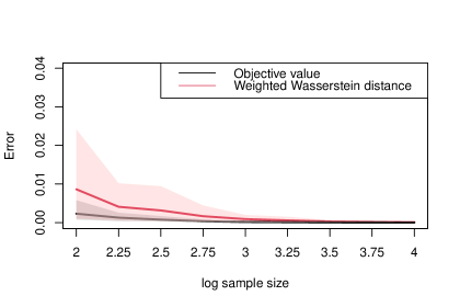
Figure 1: Convergence of error and weighted 2-Wasserstein distance obtained by weighted least squares regression. Black line = objective (error) of the optimization problem of weighted least squares regression. Red line = Wasserstein distance between the estimated quantile function and the true quantile function. Grey band = $90$% confidence band of the error obtained by $100$ repeated experiments. Red band = $90$% confidence band of the distance obtained by $100$ repeated experiments. The horizontal axis = sample size in log scale.

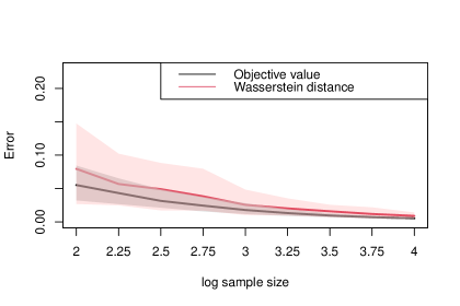
Figure 2: Convergence of error and 1-Wasserstein distance obtained by least absolute deviation regression. Black line = objective (error) of the optimization problem of weighted least squares regression. Red line = Wasserstein distance between the estimated quantile function and the true quantile function. Grey band = $90$% confidence band of the error obtained by $100$ repeated experiments. Red band = $90$% confidence band of the distance obtained by $100$ repeated experiments. The horizontal axis = sample size in log scale

8.2 Estimation of Mixture Quantiles of Generalized Beta Distributions with Financial Market Drawdowns

This section applies the model to a real-life data set. We fit the mixture quantiles of generalized beta distributions of the second kind to the log market drawdowns. This case study is inspired by Frey (2021) which finds that the lomax distribution has a good fit for market drawdowns. Drawdowns are calculated with 40-year historical adjusted close price of the SP500 Index from 01/01/1982 to 01/01/2022.

Financial Market Drawdowns

Drawdown financial characteristics is the the security price drop from the previous highest value in percentage. Suppose we have a time series of security price, $p_{t}$, $t=1,\cdots,T$. The drawdown at time $t$ is defined by $d_{t}=(\max_{i\in\{1,\cdots,t\}}p_{i}-p_{t})/\max_{i\in\{1,\cdots,t\}}p_{i}$. The security is in a drawdown at time $t$, if $p_{t}>0$. We call period $(t_{1},t_{2})$ a drawdown period if ${d}_{t}>0$ for $t_{1}<t<t_{2}$ and ${d}_{t_{1}}={d}_{t_{2}}=0$. We take the maximum drawdown in each drawdown period. SP500 Index has a total of $406$ drawdown periods from 01/01/1982 to 01/01/2022. Then, we fit a model to 406 maximum log-tranformed drawdowns.

Generalized Beta Distribution of the Second Kind

The generalized beta distribution of the second kind is defined by the following density function $f(x,\theta_{1},\theta_{2},\theta_{3},\theta_{4})=\frac{|\theta_{1}|y^{\theta_{1}\theta_{3}-1}}{b^{\theta_{1}\theta_{3}}B(\theta_{3},\theta_{4})(1+(x/\theta_{2})^{\theta_{1}})^{\theta_{3}+\theta_{4}}}$. It nests many common distributions such as the generalized gamma (GG), Burr type 3, lognormal, Weibull, Lomax, half-Student’s $t$, exponential, power function, etc. Our approach can be regarded as estimating mixture quantiles of these distributions. We first use the following grid to populate the design matrix. $\theta_{2}\in\{0.1,0.2,\cdots,1\}$, $\theta_{3}\in\{1,2,\cdots,10\}$, $\theta_{4}\in\{1,2,\cdots,10\}$. The scale parameter $\theta_{1}$ is fixed at $1$. The quantile functions are then standardized as described in Section 3. Then, to improve stability of optimization, we remove extreme values: quantile functions that either have $1/407$-quantile smaller than $10^{-4}$ or $406/407$-quantile larger than $10^{3}$. This is a reasonable choice since the scale of drawdowns varies from $10^{-2}$ to $10^{2}$. Those removed components is unlikely to be selected by the algorithm as a good fit, anyway. A total of $4792$ quantile functions are included in the initial mixture.

Optimization Setting

We minimize the error (see (4)), with non-negativity constants (see Section 7). Additionally, we impose the cardinality constraints ( see Section 7). The value of the cardinality constraint is $C=1,2$. As a comparison, we also use LASSO regression to select the quantile functions. The coefficient $\lambda$ in LASSO regression is determined as follows: $\lambda$ is increased with step $0.1$ until the cardinality (number of non-zero variables) equals $2$ and $1$. The smallest $\lambda$ that achieves the cardinality is reported. We do not use the optimal weights formula (11) in this case study, because it assigns too small weights to extreme observations. Equal weights are assigned to all observations, as we are concerned about the tail risk.

Goodness-of-fit

Table 1 presents the goodness-of-fit test statistics. We report the weighted mean squared error (WMSE), mean absolute error (MAE), Kolmogorov–Smirnov distance (KS) and log likelihood (LLK). Maximum likelihood estimate (MLE) of generalized beta distribution of the second kind is included for comparison.

	Least squares regression					Least absolute deviation regression					MLE
$\bm{C}$	N/A	2	1	N/A	N/A	N/A	2	1	N/A	N/A	N/A
$\bm{\lambda}$	N/A	N/A	N/A	0.6	1.2	N/A	N/A	N/A	1.1	1.9	N/A
WMSE	$0.21$	$0.21$	$1.04$	$0.25$	$1.88$	$0.31$	$0.31$	$0.28$	$0.70$	$3.07$	$0.40$
MAE	$0.14$	$0.16$	$0.34$	$0.24$	$0.78$	$0.10$	$0.10$	$0.26$	$0.38$	$0.74$	$0.15$
KS	$0.10$	$0.13$	$0.20$	$0.22$	$0.57$	$0.05$	$0.08$	$0.15$	$0.18$	$0.56$	$0.03$
LLK	-$381.0$	-$386.3$	-$439.4$	-$585.2$	-$737.4$	-$389.2$	-$400.6$	-$414.6$	-$518.5$	-$720.5$	-$345.4$

Table 1: The table presents the measures of goodness-of-fit for models with different errors, constraints and penalties. MLE is included for comparison. $C=$ value of cardinality constraint, $\lambda=$ coefficient of $L_{1}$ penalty in LASSO regression, WMSE = weighted mean squared error, MAE = mean absolute error, KS = Kolmogorov–Smirnov distance, LLK = log likelihood.

When the cardinality of the model is at least 2, regressions outperform MLE in terms of WMSE and MAE. The error of the optimization with cardinality constraint 2 is only slightly higher compared to the optimization without cardinality constraint. The test statistics are significantly worse with cardinality 1. MLE outperforms other models in terms of KS and LLK. In most cases, the model fitted with cardinality constraint outperforms the model fitted with $L_{1}$ penalty.

Figure 3 and 4 present the Q-Q plot of models fitted with different errors, constraints and penalties. MLE is included for comparison. The following three regressions provide close results and have good fit: 1) weighted least squares regression; 2) weighted least squares regression with cardinality constraint $C=2$; 3) weighted least squares regression with Lasso penalty coefficient $\lambda=0.6$. These models have a better fit to the tail observations than MLE. Figures 3b, 4b for MLE show that extreme tail observations are all below the straight line $y=x$, i.e., MLE underestimates the tail risk. When cardinality equals $1$, neither of the regression with cardinality constraint or with $L_{1}$ penalty has a good fit. For least absolute deviation regression, except for the regression with coefficient of $L_{1}$ penalty $\lambda=1.9$, all models are close and have good fit. They have better fit to the tail observations than MLE. Log probability plot in Appendix A directly compares the models in one graph.

(a) Weighted least squares

(b) MLE

(c) Cardinality constraint $C=2$

(d) Cardinality constraint $C=1$

(e) LASSO $\lambda=0.6$

(f) LASSO $\lambda=1.2$

Figure 3: Q-Q plots of models fitted by least squares regression with cardinality constraint $C=1,2$ and coefficient $\lambda=0.6,12$ of $L_{1}$ penalty. MLE is included as a benchmark. $\{(x_{n},y_{n})\}_{n=1}^{N}$ = black points, $x_{n}=$ $n$-th sample order statistics, $y_{n}=$ quantile with confidence level $\frac{n}{N+1}$ of the model.

(a) Least absolute deviation

(b) MLE

(c) Cardinality constraint $C=2$

(d) Cardinality constraint $C=1$

(e) LASSO $\lambda=1.1$

(f) LASSO $\lambda=1.9$

Figure 4: Q-Q plots of models fitted by least absolute deviation regression with cardinality constraint $C=1,2$ and coefficient $\lambda=1.1,1.9$ of $L_{1}$ penalty. MLE is included as a benchmark. $\{(x_{n},y_{n})\}_{n=1}^{N}$ = black points, $x_{n}=$ $n$-th sample order statistics, $y_{n}=$ quantile with confidence level $\frac{n}{N+1}$ of the model.

9 Conclusion

We proposed a flexible parametric model for the quantile function. The model can be efficiently fitted using constrained linear regression. We studied various properties of the estimator. We proved that the estimator is asymptotically the minimum Wasserstein estimator. Also, we proved the asymptotical normality of the estimator. We suggested constraints and penalties for the regression optimization problem to improve performance of the estimator. Numerical experiments demonstrated that the suggested models have a good fit to tail observations. Also, experiments demonstrated that test statistics of weighed mean squared error and mean absolute error outperformed maximum likelihood estimation. We observe, that the model with cardinality constraint outperforms the model with $L_{1}$ penalty. The proposed model can be generalized to other risk functions, such as Conditional Value-at-Risk (CVaR, Rockafellar and Uryasev (2000, 2002)) and expectile (Newey and Powell, 1987), which are popular in finance and engineering.

Appendix A Comparison of Scaled Quantile Functions of Fitted Models

The Appendix presents two log probability plots summarizing numerical case study in Section 8.2. The quantile functions of different models fitted by minimizing the same error are compared in one graph. The x-axis is log-transformed for better visualization of tail behavior.

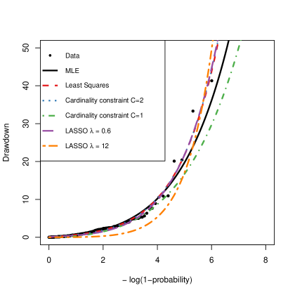
Figure 5: Scaled quantile functions of the fitted models and sample points $\{(-\log(1-p_{n}),y_{n})\}_{n=1}^{N}$, where $p_{n}=\frac{n}{N+1}$ and $y_{n}$ are the standardized drawdowns. The y-axis is the standardized drawdown. The x-axis is -log(1-probability). The models are fitted with least squares regression with cardinality constraint $C=1,2$ and coefficient $\lambda=1.1,1.9$ of $L_{1}$ penalty. The following three estimates almost overlap: least squares, least squares with cardinality constraint $C=2$, and least squares with penalty coefficient $\lambda=0.6$. Compared to MLE, all models have better fit to the tail observations, except for least squares regression with $C=1$.

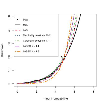
Figure 6: Scaled quantile functions of the fitted models and sample points $\{(-\log(1-p_{n}),y_{n})\}_{n=1}^{N}$, where $p_{n}=\frac{n}{N+1}$ and $y_{n}$ are the standardized drawdowns. The y-axis is the standardized drawdown. The x-axis is -log(1-probability). The models are fitted with least least absolute deviation (LAD) regression with cardinality constraint $C=1,2$ and coefficient $\lambda=1.1,1.9$ of $L_{1}$ penalty. The two scaled quantile functions obtained by the following estimators almost overlap: LAD regression and LAD regression with cardinality constraint $C=2$. Compared to MLE, all models have better fit to the tail observations.

References

- Vincent (1912) Stella Burnham Vincent. The Functions of the Vibrissae in the Behavior of the White Rat…, volume 1. University of Chicago, 1912.
- Ratcliff (1979) Roger Ratcliff. Group reaction time distributions and an analysis of distribution statistics. Psychological bulletin, 86(3):446, 1979.
- Sillitto (1969) G. P. Sillitto. Derivation of approximants to the inverse distribution function of a continuous univariate population from the order statistics of a sample. Biometrika, 56(3):641–650, 1969. ISSN 00063444. URL http://www.jstor.org/stable/2334672.
- Karvanen (2006) Juha Karvanen. Estimation of quantile mixtures via l-moments and trimmed l-moments. Computational Statistics & Data Analysis, 51(2):947–959, 2006. ISSN 0167-9473. doi: https://doi.org/10.1016/j.csda.2005.09.014. URL https://www.sciencedirect.com/science/article/pii/S0167947305002513.
- Keelin and Powley (2011) Thomas W. Keelin and Bradford W. Powley. Quantile-parameterized distributions. Decision Analysis, 8(3):206–219, 2011. doi: 10.1287/deca.1110.0213. URL https://doi.org/10.1287/deca.1110.0213.
- Ramsay (1988) J. O. Ramsay. Monotone regression splines in action. Statistical Science, 3(4):425–441, 1988. ISSN 08834237. URL http://www.jstor.org/stable/2245395.
- Papp (2011) Dávid Papp. Optimization models for shape-constrained function estimation problems involving nonnegative polynomials and their restrictions. 2011.
- Papp and Alizadeh (2014) Dávid Papp and Farid Alizadeh. Shape-constrained estimation using nonnegative splines. Journal of Computational and Graphical Statistics, 23(1):211–231, 2014. doi: 10.1080/10618600.2012.707343. URL https://doi.org/10.1080/10618600.2012.707343.
- LaRiccia (1982) Vincent N. LaRiccia. Asymptotic properties of weighted quantile distance estimators. The Annals of Statistics, 10(2):621 – 624, 1982. doi: 10.1214/aos/1176345803. URL https://doi.org/10.1214/aos/1176345803.
- Millar (1984) P. Warwick Millar. A general approach to the optimality of minimum distance estimators. Transactions of the American Mathematical Society, 286:377–418, 1984.
- Gilchrist (2007) Warren G. Gilchrist. Modeling and fitting quantile distributions and regressions. American Journal of Mathematical and Management Sciences, 27(3-4):401–439, 2007. doi: 10.1080/01966324.2007.10737707. URL https://doi.org/10.1080/01966324.2007.10737707.
- Bassetti and Regazzini (2006) Federico Bassetti and Eugenio Regazzini. Asymptotic properties and robustness of minimum dissimilarity estimators of location-scale parameters. Theory of Probability and Its Applications, 50:171–186, 2006.
- Bassetti et al. (2006) Federico Bassetti, Antonella Bodini, and Eugenio Regazzini. On minimum kantorovich distance estimators. Statistics & Probability Letters, 76(12):1298–1302, 2006. ISSN 0167-7152. doi: https://doi.org/10.1016/j.spl.2006.02.001. URL https://www.sciencedirect.com/science/article/pii/S0167715206000381.
- Bernton et al. (2019) Espen Bernton, Pierre E Jacob, Mathieu Gerber, and Christian P Robert. On parameter estimation with the Wasserstein distance. Information and Inference: A Journal of the IMA, 8(4):657–676, 10 2019. ISSN 2049-8772. doi: 10.1093/imaiai/iaz003. URL https://doi.org/10.1093/imaiai/iaz003.