Principle of Information Increase: An Operational Perspective of Information Gain in the Foundations of Quantum Theory

Abstract

A measurement performed on a quantum system is an act of gaining information about its state. This viewpoint is widely held both in practical applications and foundational research. In the former, the applications treat information theory as a pure mathematical tool; while in the latter, information plays a central role in many reconstructions of quantum theory. However, the concept of information in quantum theory reconstructions is usually remained obscure. We are investigating the information towards the reconstruction of quantum theory from an operational approach: what is the information gained from the data of measurements on quantum systems. It is found that there are situations that classical information measures are not applicable. We start from the discussion of the generalization of continuous entropy and find that there is more than one natural measure of the information gained as more data is received. One of these (differential information gain) can increase or decrease with more data, depending upon the prior; another measure (relative information gain) is an increasing function of the amount of data even when the amount of data is finite, and is asymptotically insensitive to the specific data or choice of prior. All these two measures can be regarded as extensions of relative entropy, the relation with expected information gain is also discussed.

We propose a foundational principle from an intuitive idea: “more data from measurements lead to more knowledge about a physical quantity”, which was first proposed by Summhammer [1, 2]. This idea is reformulated in terms of information theory as a Principle of Information Increase to investigate the information gain from data of quantum measurements. This principle is used as a criterion to filter the choices of prior for the prior-sensitive information measures. Both numerical and asymptotic analysis are conducted based on the family of beta distribution priors. It is showed that in two-outcome quantum systems differential information gain will be more physical meaningful under this principle and Jeffreys’ binomial prior exhibits a special behavior which is the strong robustness of information gain over all possible data sequences. In the case of expected information gain, the expected values of two measures are equal to each other, which suggests that the form is unique and the discrepancies are disappeared when taking the averages.

1 Introduction

A measurement performed on a quantum system is an act of gaining information about its state. This viewpoint is widely held both in practical situations and in foundational research. In the former, applications as diverse as quantum tomography [3, 4, 5, 6], Bayesian experimental design [7], and informational analysis of experimental data [8, 9], information is used to generate a utility function, which is extremized to find an optimal parameter. While in the latter, information plays a central role in many reconstructions of quantum theory, which seek to distill the mathematical content into a set of information-inspired postulates [10, 11, 12, 13, 14, 15, 16, 17, 18]. However, in research of the foundations of quantum theory, the concept of information is formalized in many different ways. This raises the question of whether there is a more principled basis for choosing how to formalize the information concept in such an arena. A clear definition of information is the cornerstone when reconstructing quantum theory from informational approaches. In this paper, we want to examine the concept of information from an operational viewpoint, a physically intuitive postulate is proposed to determine a proper information gain from measurements.

In both tomography applications and reconstructions of quantum theory, we may focus on the probability distributions of physical parameters. Once we take measurements about a physical quantity, our knowledge of this quantity will be updated from the measurement results. For example, the probability distribution $Pr(x|D)$ of a quantity $x$ updated via results $D$ of a collection of identical measurements. It is natural to think about using Shannon entropy of this updated distribution to measure the information obtained. Yet Shannon entropy is only defined over discrete distributions, while physical quantity or the probability distribution may be continuous.

It is a question that what is a proper measure to evaluate the amount of information gained from real data, especially for quantities which are associated with continuous probability distributions. And we still want to find some measures based on Shannon entropy, due to its well-established axiomatization. One possible solution is to use Kullback-Leibler (KL) divergence, which is also called relative entropy, $H(x|D)=\int Pr(x|D)\ln\frac{Pr(x|D)}{Pr(x|I)}dx$, where $Pr(x|I)$ is the prior distribution of $x$ and $Pr(x|D)$ is the posterior of $x$ updated via receiving the data $D$. This quantity is also called the information gain from prior to posterior.

The KL divergence solves the problem of differential entropy, it is non-negative and invariant under change of coordinates. However, there are situations that information gain has no unique forms. Consider the case that we have obtained a series of data $D$ and if we take subsequent measurements obtaining another data $D^{\prime}$, what’s the information gain about data $D^{\prime}$? Based on KL divergence, we have two ways to represent the information about this additional data. The first is differential information gain, which is the difference of information gain of whole data $\{D,D^{\prime}\}$ and the information gain from $D$; the second is relative information gain, which contains only one term, the KL divergence of posterior after receiving the whole data $\{D,D^{\prime}\}$ to posterior of receiving data $D$ only. These measures of information gain exhibit markedly different behaviors. For example, whether the differential information can increase or decrease depends on the choice of prior over the bias, whereas the relative information is positive irrespective of prior. The origin of two measures may date back to the generalization of Shannon entropy to continuous distributions. In Sec. 2 we will discuss the problem of continuous entropy, it turns out both of the two measures can be regarded as the consequences of the continuous entropy.

It is natural to think about which information gain should we use, and we want to introduce a physically intuitive informational postulate to select the choice between them. The first criterion comes from an intuitive idea that “more data from measurements lead to more knowledge about the system” [1, 2]. For example, if we perform more and more measurements about the value of a physical quantity, the measurement uncertainty would be decreased which means we may obtain more knowledge about this quantity. We want to use information theory to formalize this idea and information gain is used to quantify the knowledge about a quantity. As the idea suggested, information gain of the additional data should be positive. It seems that the relative information gain could be a better choice since it’s always non-negative while the positivity of differential information gain depends on the choice of prior.

However, it turns out the negative information gain is meaningful and even necessary. Consider the case of black swan event, the emergence of a black swan may significantly increase people’s uncertainty about the color of the swan. Our discussion of information begins from Shannon entropy and gaining information is regarded as a process of reducing degree of uncertainty, and the information gain from this black swan observation should be negative. These two intuitive scenarios lead to the Principle of Information Gain: information gain of the additional data should be positive asymptotically and negative under extreme cases.

The Principle of Information Gain suggests that differential information gain is more meaningful, it also provides a certain range of priors from beta distribution family. We notice that a special choice of the prior could be picked from this range, by introducing another criterion, robustness of information gain over the previous data. If the result of additional data $D^{\prime}$ is fixed, then for different $D$, the information gain due to $D^{\prime}$ will be different. The robustness is used to describe the difference of information gain over all possible data $D$. It is found that the Jeffreys’ prior shows the strongest robustness over all other beta distributions priors.

The situation of quantifying knowledge of the additional data is rarely investigated. In the research of foundations of quantum theory, this problem is noticed but addressed coarsely. Summhammer first proposes the idea that “more data from measurements lead to more knowledge about the system”. However, Summhammer doesn’t employ information theory to deal with this problem, instead he uses the change of measurement uncertainty to quantify the knowledge from measurements. This restricts the usage of this idea, which can only be applied asymptotically.

Wootters [19] shows the importance of Jeffreys’ prior for quantum system from another information-theoretical approach. In the problem of communication through quantum systems, the Jeffreys’ prior may lead to obtaining the maximal information from measurements. Wootters treat the information more systematically, and mutual information is used to measure the information from measurements. Yet mutual information is taking the average of the information gain of all possible data sequence. It is not helpful in the situation we discussed above, we are dealing with information gain from a fixed data sequence.

In both practical applications and in foundational research on quantum theory, the question of how much information is gained as additional data is obtained has received little attention. Commonly, the mutual information is used as a utility function. But the mutual information is effectively an expected information gain over all possible data sequences. So, the question of how much information is gained if a given additional datum is obtained does not arise. However, from our vantage point, this averaging process wipes out important edge effects, such as “Black Swan Events”, which (as we shall see) are important guides in the selection on appropriate information measures.

Although our investigation mainly focus on the information gain on quantum systems, this approach and conclusion can be extended to a general probabilistic system characterized by fixed continuous parameters. On the basis of our analysis, quantification via differential information gain, and use of the Jeffreys’ prior, is recommended. If one wishes to calculate the expected information gain on the next step, then one can take either the expected differential information gain or the expected relativity information, because (as we show) they are equal.

In the area of dealing with consecutive data sequences, we provide an approach of calculating the information gain on each step. In particular, we have shown that the expected value of differential information gain and relative information gain are equal. This suggests that if people are interesting on the expected information gain on the next step, there is no divergence on this expected quantity and the value should be unique.

This paper is structured as below. In Sec. 2 we will introduce the detailed definition of the two information gain, both of them are originated from the generalization of Shannon entropy to continuous distributions. The Jaynes’ approach to continuous entropy is discussed, the two information gain can be regarded as the consequences of this approach. In Sec. 3 and Sec. 4 we will discuss the numerical and asymptotic analysis of differential information gain and relative information gain respectively. We mainly focus on the behavior of the two information under different priors. The extreme case of “Black Swan Event” where the additional data $D^{\prime}$ is highly improbable given $D$ . Under this special situation we may be able to evaluate the physical meaningfulness of the two information gain. In Sec. 5 we will discuss the expected information gain under the situation that the data $D^{\prime}$ of the additional measurements haven’t been received. Though the two measures are generally different to each other, the two expected information gain are surprisingly mutually agreed. Sec. 6 provides a comparison of the two information gain and the expected information gain, the Principle of Information Gain is proposed under the results of the two information gain’s analysis. Sec. 7 shows the relation with other people’s work.

2 Continuous Entropy and Bayesian Information Gain

2.1 Entropy of Continuous Distribution

The Shannon entropy can be regarded as measure of uncertainty about a random variable before we know about its value. If treating information as the complementary component to uncertainty, the Shannon entropy can also be used as a measure of information gain after we learn its value. However, Shannon entropy only works for discrete random variables. Shannon proposes differential entropy as the extension of entropy for continuous variables. Unlike Shannon entropy, the differential entropy cannot be derived from axioms and there are some weaknesses. The differential entropy could be negative, for example the differential entropy of a uniform distribution on interval $[0,\frac{1}{2}]$ is $-\log 2$. The negative degree of uncertainty is not meaningful. Moreover, the differential entropy is coordinate dependent [20], the value is not conserved under change of variables. This means we may have different degree of uncertainty in different coordinate, which is also not meaningful.

Jaynes [21] proposes a solution to continuous entropy, in an approach called limiting density of discrete points (LDDP). Assume the probability density $p(x)$ of random variable $X$ is initially defined on a set of discrete points $x\in\{x_{1},x_{2},\cdots,x_{n}\}$. Jaynes proposes an invariant measure $m(x)$ such that when the collection of points $\{x_{i}\}$ becoming more and more numerous, in the limit $n\rightarrow\infty$,

$$\lim_{n\rightarrow\infty}\frac{1}{n}\text{~{}(number of points in~{}$a<x<b$)}=\int_{a}^{b}m(x)dx$$ (1)

With the help of $m(x)$, the entropy of $X$ can then be represented as

$$H(X)=\lim_{n\rightarrow\infty}\log{n}-\int p(x)\log\frac{p(x)}{m(x)}dx$$ (2)

In this way, the weaknesses of differential entropy seems to be solved, this quantity is invariant under the change of variables and it is non-negative. Similar procedure is also discussed in Ref.[20]. However, there are two new problems. $H(X)$ in equation 2 contains an infinity term and the measure function $m(x)$ is unknown.

For the infinity term, there could be two solutions. The first is that we can reserve this infinity term, and the entropy of continuous distribution is only meaningful when we consider the difference of two entropy. The second solution is more straightforward, just drop the $\log n$ term to avoid infinity.

1. Entropy of continuous distribution as a difference

   For example, when variable $X$ is updated to $X^{\prime}$ due to some actions, the decrease of entropy will be equal to

   $$X\rightarrow X^{\prime},\quad\Delta H(X\rightarrow X^{\prime})=H(X^{\prime})-H(X)=\int p^{\prime}(x)\log\frac{p^{\prime}(x)}{m(x)}dx-\int p(x)\log\frac{p(x)}{m(x)}dx$$ (3)

   where $p^{\prime}(x)$ is the probability distribution of $X^{\prime}$. Here we assume the two infinity terms are canceled out. The quantity $\Delta H$ quantifies the loss of uncertainty about variable $X$ in this action. The loss of uncertainty can also be regarded as the gain of information.

2. Straightforward

   Jaynes directly drops the infinity term in equation (2). For the sake of convenience, the minus sign is also dropped. Then we may have the Shannon-Jaynes information

   $$H_{Jaynes}(X)=\int p(x)\log\frac{p(x)}{m(x)}dx$$ (4)

   This term quantifies how much information we know about the outcome of $X$, rather than the degree of uncertainty of $X$. $H_{Jaynes}$ is just equal to the KL divergence of $p(x)$ to $m(x)$.

Now there are two ways to represent the entropy of continuous distribution. There is no preference of them. In the special case that if variable $X$ initially has distribution the same with measure function $p(x)=m(x)$ and $X$ is evolved into $X^{\prime}$ with distribution $p^{\prime}(x)$, then $\Delta H(X\rightarrow X^{\prime})=H_{Jaynes}(X^{\prime})$.

The remained problem is the choice of measure function $m(x)$. When applying this continuous entropy into the relation between information theory and statistical physics, Jaynes chooses measure function as a uniform function. Yet this choice may not be applied into other situations. Currently we don’t have any criterion of this choice of measure function. Noticing that this measure function acting like the prior distribution in Bayesian probability framework. In the following discussion we may focus on the application of Bayesian information gain, where the measure function $m(x)$ can be interpreted as the prior of the target variable.

2.2 Bayesian Information Gain

In a coin tossing model, let $p$ be the probability of head in a single toss and $N$ be the total number of tosses. After $N$ tosses, the results of $N$-tosses is represented by a $N$-tuple $T_{N}=(t_{1},t_{2},\cdots,t_{N})$ where $t_{i}$ is the result of $i$th toss and $t_{i}\in\{Head,Tail\}$. By Bayes’ rule, the posterior of the probability of head would be

$$Pr(p|N,T_{N},I)=\frac{Pr(T_{N}|N,p,I)Pr(p|I)}{\int Pr(T_{N}|N,p,I)Pr(p|I)dp}$$ (5)

where $Pr(p|I)$ is the prior probability. The information gain after $N$ tosses would be the KL divergence from prior to the posterior:

$$I(N)=D_{KL}(Pr(p|N,T_{N},I)||Pr(p|I))=\int^{1}_{0}Pr(p|N,T_{N},I)\ln{\frac{Pr(p|N,T_{N},I)}{Pr(p|I)}}dp$$ (6)

From the above discussion of continuous entropy, this quantity can be interpreted as obtained from two ways: 1) the difference of information gain after $N$ tosses and information gain without any tosses; 2) from straightforward method, just take the KL divergence of posterior to the prior.

It is more complex to consider the information gain of more tosses based on the results of previous $N$ tosses. We may find that there are two different ways of representing this quantity.

Let $t_{N+1}$ be the result of the $N+1$th toss and $T_{N+1}=(t_{1},t_{2},\cdots,t_{N},t_{N+1})$. The posterior after these $N+1$ tosses would be:

$$Pr(p|N+1,T_{N+1},I)=\frac{Pr(T_{N+1}|{N+1},p,I)Pr(p|I)}{\int Pr(T_{N+1}|{N+1},p,I)Pr(p|I)dp}$$ (7)

If taking the idea of information gain as a difference between two quantities. The first form of information gain of this single toss $t_{N+1}$ would be

$$I_{diff}=D_{KL}(Pr(p|N+1,T_{N+1},I)||Pr(p|I))-D_{KL}(Pr(p|N,T_{N},I)||Pr(p|I))$$ (8)

In this expression, the first term $H(Pr(p|N+1,t_{N+1},I)||Pr(p|I))$ is the information gain from $0$ tosses to $N+1$ tosses and the second term $H(Pr(p|N,T_{N},I)||Pr(p|I))$ is the information gain from the $0$ tosses to $N$ tosses, the difference between them is the information gain in the single $N+1$th toss. In this sense we would call $I_{diff}$ be the “differential information gain in a single toss”.

Figure 1: The first form of information gain in single toss. Assume we have the data of $N$ tosses, $T_{N}$. By using certain prior, we could calculate the information gain in the first $N$ tosses, $I(N)$. If we take $N+1$th toss and the result is $t_{N+1}$, we can repeat the same procedure to calculate the information gain in total $N+1$ tosses, $I(N+1)$. The information gain in the $N+1$th toss will be the difference of $I(N+1)$ and $I(N)$.

Or we could take the straightforward idea. The second form would be

$$I_{rel}=D_{KL}(Pr(p|N+1,T_{N+1},I)||Pr(p|N,T_{N},I))$$ (9)

We calculate the information gain from $N$th toss to $N+1$th toss (the KL divergence from posterior after $N$ tosses to posterior after $N+1$ tosses). We would call $I_{rel}$ be the “relative information gain in a single toss”.

Figure 2: The second form of information gain in single toss. The posterior calculated from the first $N$ tosses acting like the prior of the $N+1$th toss. The KL divergence between the posterior and post-posterior now represent the information gain in the $N+1$th toss.

In general these two quantities are not the same unless $N=0$, which means no measurements have already performed. $I_{diff}$ could be negative while $I_{rel}$ is always non-negative due to the property of KL divergence. KL divergence is not a proper distance between two probability distributions, since it doesn’t satisfy the triangle inequality, yet it’s very useful to take the analogy of the displacement and distance in random walk model to show the subtle difference between the two information gain. The differential information gain is acting like the displacement from $N$th step to $N+1$th step relative to the origin, so it could be positive or negative; while relative information gain resembles to the distance between $N$th step to $N+1$th step, which is always non-negative.

We are interested in which information gain is a better choice to be used, and we want to introduce an informational postulate to make a choice. This postulate comes from an intuitive idea, “more measurements lead to more knowledge about the physical system” [1, 2]. For example when measuring the value of a physical quantity, we tend to make more identical measurements to eliminate the statistical fluctuation of the values. We may wonder whether this idea can be reformulated in terms of information theory. If “knowledge” is quantified with information gain from data and this idea is valid, then it seems that the information gain of the additional data should be positive. This suggests that relative information gain could be a better choice, since it is always non-negative. However, the derivation of differential information gain is also meaningful. This raises a question whether this idea is physically meaningful, if not what’s the reasonable version of this idea? In the following sections we will first investigate the differential information gain on both finite $N$ case and asymptotic case. The meaning of negative value of information gain, especially for extreme cases, is discussed. The numerical and asymptotic analysis of relative information gain is also presented. After the analysis of the two information gain, we may be able to take the comparison and relations between them as well as the physical meaningfulness of the intuitive idea.

3 Differential Information Gain

3.1 Finite number of tosses

The prior we are using is the beta distribution, since the beta distribution is the conjugate prior of the binomial distribution.

$$Pr(p|I)=\frac{p^{\alpha}(1-p)^{\alpha}}{B(\alpha+1,\alpha+1)}$$ (10)

where $\alpha>-1,B(\cdot,\cdot)$ is the beta function.

In general, the beta distribution has two parameters. For the sake of convenience we only use one parameter. The family of single parameter beta distribution already covers a wide range of priors, for example uniform distribution ($\alpha=0$) and Jeffreys’ prior ($\alpha=-0.5$) are included in this range.

The differential information gain of the $N+1$th toss is (see appendix A)

$$I_{diff}={} \psi(h_{N}+\alpha+2)-\psi(N+2\alpha+3)+$$ (11)

$$\frac{h_{N}}{h_{N}+\alpha+1}-\frac{N}{N+2\alpha+2}+\ln{\frac{N+2\alpha+2}{h_{N}+\alpha+1}}$$

here we assume $t_{N+1}=``Head"$. In fact there will be $I_{diff}(t_{N+1}=``Head")$ and $I_{diff}(t_{N+1}=``Tail")$ but we only need to discuss one situation, since our calculation will consider all different $T_{N}$ and the expression of these two quantities are symmetric.

$I_{diff}$ is a function of $h_{N}$ and $\alpha$ and $h_{N}$ is ranging from 0 to $N$. We will fix a value of $\alpha$ and calculate all the $N+1$ values of $I_{diff}$ for each $N$.

3.1.1 Positivity of $I_{diff}$

Back to our original question: “will more data leads to more knowledge?” If we use the differential information gain to denote term “knowledge” and $I_{diff}$ quantify the information gained in every single measurement, then question becomes quite simple: “will $I_{diff}$ be always positive?”

In Fig. 3, we show the result of numerical calculations for different $N$. By inspection of the graph, one can see that the answer is generally no except under some conditions. In the following we will explore what condition lead to exceptions.

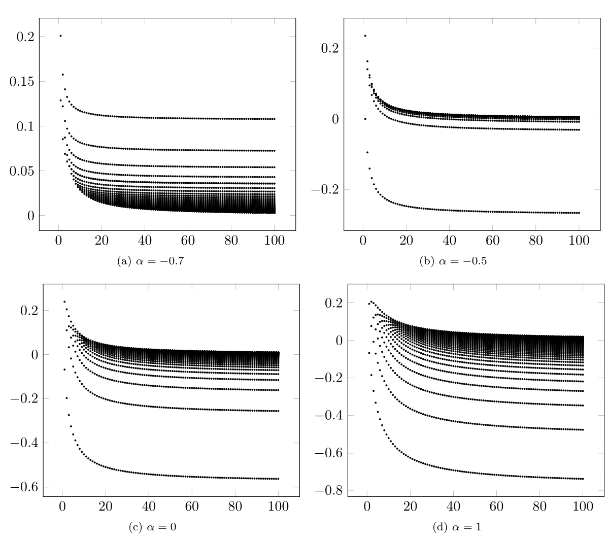
Figure 3: Differential information gain ($I_{diff}$) vs. $N$ for different priors. $I_{diff}$ is a function of $N$, $h_{N}$, and $\alpha$. In this set of graphs, Y-axis is the value of $I_{diff}$ and X-axis is the value of $N$. We fix $\alpha$ in each individual graph so that we can compare behavior of $I_{diff}$ under different priors. Given $N$, there are $N+1$ points since $h_{N}$ ranged from 0 to $N$. It is clear that for $\alpha=-0.7$ all points are above x-axis while for other priors negative points always exist. Moreover it seems that as $\alpha=-0.5$ the graph would be the most concentrating, while for $\alpha<-0.5$ and $\alpha>-0.5$ the graph becomes very dispersive. This dispersive/concentrating feature can be clearly seen in Fig. 6.

For certain priors, the differential information gain is always positive (Fig. 3(a)); while for some other priors, there are both positive and negative parts (Fig. 3(b)(c)(d)). Noticing that for priors that lead to negative parts, the bottom line is more dispersed than other data lines. This bottom line represents the case that first $N$ tosses are all tails and the $N+1$th toss is head. This situation is just the “Black Swan Event”, and negative information gain in this extreme case is in fact very meaningful. If we toss a coin $N$ times and obtains all tails, it is natural to think about that this coin is extremely biased, or even this coin has two tails with no head, and we may anticipate another tail in the next toss. The $N+1$th toss is head will raise our degree of uncertainty of the prediction in the next toss’ result, hence the information is reduced.

3.1.2 Fraction of Negatives

In order to illustrate the difference of positivity of information gain under different priors it is needed to introduce a quantity called fraction of negatives (FoN), which is the ratio of number of $h_{N}$ which lead to negative $I_{diff}$ and $N+1$. For example, for some $\alpha$, if $N=10$ and $I_{diff}<0$ when $h_{N}=0,1,2,3$, then the FoN under this $\alpha$ and $N$ is $\frac{4}{11}$.

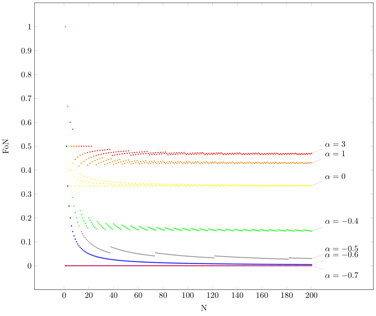
Figure 4: Fraction of Negatives (FoN) vs. $N$ under different $\alpha$. In Fig. 3 we can see that large $\alpha$ lead to more dispersive lines as well as more negative values for each $N$. We use FoN to quantify such a fraction of negative points. It seems that for $\alpha\leq-0.7$ FoN will always be zero which means $I_{diff}$ are all positive, for $\alpha\leq-0.5$ FoN is decreasing and tend to be zero in large $N$, for $\alpha>-0.5$ FoN tend to be a constant in large $N$ and this constant is increasing as $\alpha$ increasing.

From Fig. 4, we find that there exists a critical point $\alpha_{p}$ which is roughly $-0.7$ such that for any $\alpha\leq\alpha_{p}$, $I_{diff}$ will always be positive for all $N$ and $h_{N}$.

If $\alpha>\alpha_{p}$, negative terms always exist for some $h_{N}$. However, the patterns of these negative terms are not the same for different $\alpha$.

We also notice that there exists a turning point $\alpha_{0}=-0.5$ where for $\alpha\leq\alpha_{0}$, the FoN has a trend to be zero as $N$ increases, while for $\alpha>\alpha_{0}$, the FoN will tend to a constant as $N$ increases.

The critical point and turning point would be more clear in Fig. 5, the critical point $\alpha_{p}$ is very close to $-0.68$.

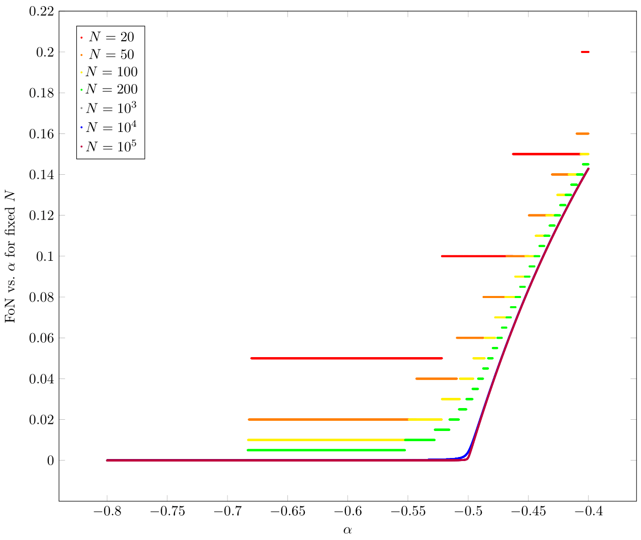
Figure 5: Fraction of Negatives (FoN) vs. $\alpha$ for different $N$. There exists a critical point $\alpha_{p}$ such that $\text{FoN}=0$ when $\alpha<\alpha_{p}$. The critical point slowly changes with respect to $N$: (i) for small $N$, $\alpha_{p}$ is close to $-0.68$; (ii) for large $N$ $\alpha_{p}$ tends to $-0.5$.

3.1.3 Robustness of $I_{diff}$

In Fig. 3, different priors not only show different patterns of positivity but also the “divergence.” More “divergent” means for different $h_{N}$, the $I_{diff}$ differs a lot. Such differences result a significant dependence of $I_{diff}$ on $h_{N}$. Since different priors show different dependence, we want to know how this dependence changes when prior changes.

The dependence of $I_{diff}$ on $h_{N}$ can be described by the standard deviation of $I_{diff}$ over different $h_{N}$. In Fig. 6, we show how standard deviation changes upon $\alpha$ under fixed $N$.

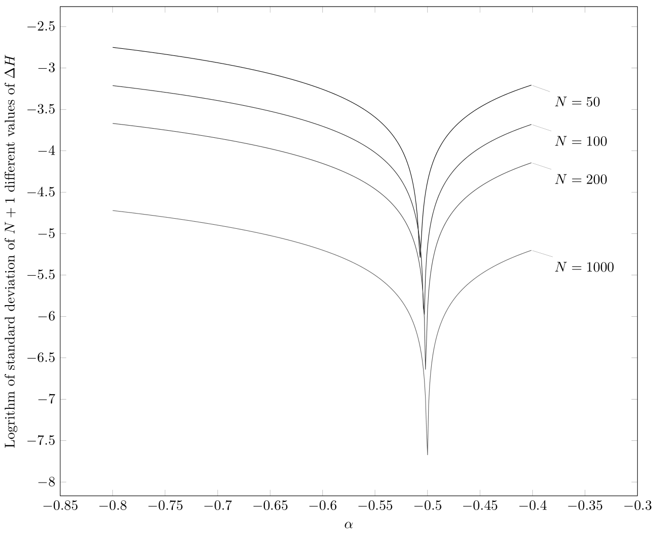
Figure 6: Robustness of differential information gain ($I_{diff}$). Y-axis denotes the logarithm of standard deviation of $I_{diff}$ over all possible $h_{N}$, X-axis denotes the different choices of $\alpha$. Smaller standard deviation would show that different $h_{N}$ lead to a same value which means $I_{diff}$ will be more independent $h_{N}$. Such independence imply that $I_{diff}$ is robust about nature since we regard $h_{N}$ is only determined by nature. Given $N$ the standard deviation is strongly influenced by $\alpha$ and there exists a point of $\alpha$ which has minimal dependence on $h_{N}$. Such a point is closing to $-0.5$ when $N$ increasing.

It is clear that when $\alpha$ near $-0.5$ the standard deviation will be the smallest. The less dependence of $I_{diff}$ on $h_{N}$, the more robust of $I_{diff}$ against nature. Since we regard $h_{N}$ is determined by nature while $N$ is determined by the man who take measurements. As $N$ increase, the closer of the minimum point to $-0.5$. In the large $N$ approximation, such a minimum point will eventually be $\alpha=-\frac{1}{2}$, which means under this choice of prior $I_{diff}$ depends least on $h_{N}$ but only on $N$.

3.2 Large $N$ approximation

By using recurrence relation and the large $x$ approximation, the digamma function can be approximated by

$$\psi(x)=\frac{1}{x-1}+\psi(x-1)\approx\frac{1}{x-1}+\ln(x-1)-\frac{1}{2(x-1)}=\frac{1}{2(x-1)}+\ln(x-1)$$ (12)

Hence the large $N$ approximation for differential information gain in (11) will be

$$I_{diff}=\frac{2h_{N}+1}{2(h_{N}+\alpha+1)}-\frac{2N+1}{2(N+2\alpha+2)}$$ (13)

It is clear that in the case $\alpha=-\frac{1}{2}$, $I_{diff}=\frac{1}{2(N+1)}$, which means $I_{diff}$ only depends on $N$. This result agrees with the Fig. 3 that $I_{diff}$ are most concentrating for $\alpha=-0.5$ and the result of [22].

In Fig. 4 we can see that the FoN tend to be constant for very large $N$. Those constants can also be estimated using the large $N$ approximations of $I_{diff}$ in (13).

Let $I_{diff}\leq 0$ we get

$$\text{if }h_{N}\leq\frac{2N\alpha+N+\alpha+1}{4\alpha+3}\quad\text{ then }I_{diff}\leq 0$$ (14)

The FoN would be

$$\text{FoN}=\frac{\frac{2N\alpha+N+\alpha+1}{4\alpha+3}}{N+1}\approx\frac{2\alpha+1}{4\alpha+3}$$ (15)

which agrees with the asymptotic lines in Fig. 4 and supports the assumption proposed in Fig. 3.

$\alpha$	FoN (numerical result with $N=1000$)	FoN (asymptotic result)	discrepancy between two results
-0.7	0	0	0
-0.6	0.001	0	$0.1\%$
-0.5	0.013	0	$1.3\%$
-0.4	0.144	0.143	$0.1\%$
0	0.334	0.333	$0.1\%$
1	0.429	0.429	0
3	0.467	0.467	0

Table 1: Fraction of negatives (FoN) under selected priors. Comparison between numerical results and asymptotic results show that they agree with each other

4 Relative Information Gain

The second form of information gain in a single toss is relative information gain, which is the KL divergence from the posterior after $N$ tosses to the posterior after $N+1$ tosses. We still use the one parameter beta distribution prior in the form of (10) and the relative information gain would be (see appendix B for the details of calculation)

$$I_{rel}(t_{N+1}=``Head")=\psi(h_{N}+\alpha+2)-\psi(N+2\alpha+3)+\ln{\frac{N+2\alpha+2}{h_{N}+\alpha+1}}$$ (16)

The relative information gain behaves totally different with differential information gain. Due to the property of KL divergence, the relative information gain is always non-negative, there’s no need to discuss the fraction of negatives. We want to see the dependence of relative information gain on priors, as well as the meaning of information gain in the extreme cases.

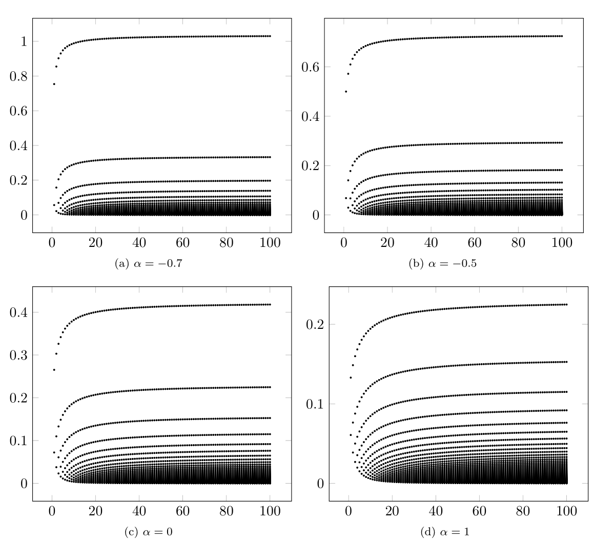
Figure 7: Relative information gain ($I_{rel}$) over different priors. Y-axis is the value of $I_{rel}$ and X-axis is $N$. For each $N$ there are $N+1$ different values of $I_{rel}$. Obviously $I_{rel}$ is positive under these choices of priors. Similar to differential information gain, every graph has many divergent lines. Yet the shape of these divergent lines are very similar over different $\alpha$, and majority of the lines are located in the range of $I_{rel}$ between $0$ and $0.2$.

From Fig. 7, we may find that under different priors, the data lines have similar shape, this may indicate that relative information gain is insensitive to the choice of priors. On each graph, the top line is the extreme case that first $N$ tosses are tails and $N+1$th toss is head. This line separates with other data lines more far away. This suggests that relative information gain acts more like the degree of surprise of this additional data. In this “Black Swan Event”, the posterior after $N+1$ tosses differs a lot to the posterior after $N$ tosses.

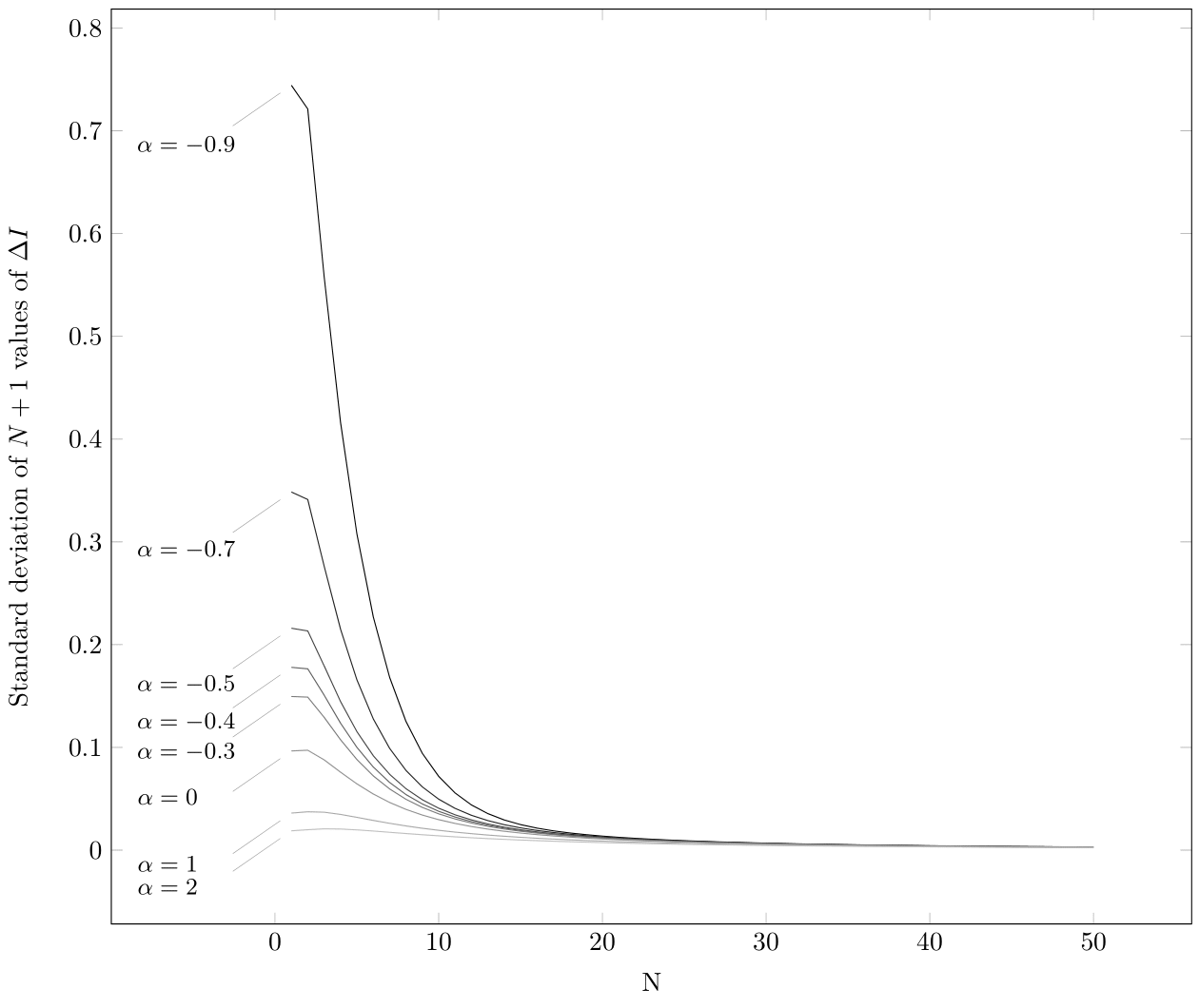
Figure 8: Robustness of relative information gain ($I_{rel}$). Y-axis is the standard deviation of $I_{rel}$ over all possible $h_{N}$. This shows the strong independence of $I_{rel}$ about $h_{N}$. As $N$ increases, the standard deviations tend to be zero under all priors.

In small $N$, both the average value and standard deviation of $I_{rel}$ shows monotonicity of $\alpha$, where larger $\alpha$ will lead to smaller average value and standard deviation. For large $N$, all priors are becoming indistinguishable. However, the relative information gain always heavily depends on data sequences ($h_{N}$). By using the approximation of digamma function we may obtain

$$I_{rel}(t_{N+1}=``Head") \approx\frac{1}{2(h_{N}+\alpha+1)}-\frac{1}{2(N+2\alpha+2)}=\frac{N-h_{N}+\alpha+1}{2(h_{N}+\alpha+1)(N+2\alpha+2)}$$ (17)

$$=\frac{\frac{\alpha}{N}+1-\frac{h_{N}}{N}}{2(\frac{h_{N}}{N}+\frac{\alpha+1}{N})(N+2\alpha+2)}$$

In the large $N$ limit $I_{rel}$ will become

$$I_{rel}(t_{N+1}=``Head")\approx\frac{N-h_{N}}{2h_{N}N}$$ (18)

It seems that the properties of relative information gain and differential information gain are complementary to each other.

	Asymptotic forms ($t_{N+1}=``Head"$)	Asymptotic sensitivity about prior
Diff Infor. Gain	$I_{diff}\approx\frac{2h_{N}+1}{2(h_{N}+\alpha+1)}-\frac{2N+1}{2(N+2\alpha+2)}$	Heavily dependent on prior and for some certain prior $I_{diff}$ will be independent of $h_{N}$
Rel Infor. Gain	$I_{rel}\approx\frac{N-h_{N}}{2h_{N}N}$	Insensitive to prior and for large $N$ only affected by $h_{N}$

5 Expected Information Gain

In this section we discuss a new situation: After $N$ tosses but $N+1$th toss hasn’t been taken. Can we “predict” how much information gain in the next toss? The answer is yes based on the above discussions.

After $N$ tosses, we get data sequences $T_{N}$ with $h_{N}$ heads. We can only estimate the probability $p$ based on the posterior $Pr(p|N,T_{N},I)$. The expected value of $p$ would be

$$\langle p\rangle=\int^{1}_{0}p~{}Pr(p|N,T_{N},I)~{}dp=\frac{h_{N}+\alpha+1}{N+2\alpha+2}$$ (19)

Based on this expected value of $p$, we could take the average of the information gain in the $N+1$th toss. First we could define the expected differential information gain in $N+1$th toss as

$$\overline{I_{diff}}= \langle p\rangle\times I_{diff}(t_{N+1}=``Head")+\langle 1-p\rangle\times I_{diff}(t_{N+1}=``Tail")$$ (20)

$$\frac{h_{N}+\alpha+1}{N+2\alpha+2}\psi(h_{N}+\alpha+2)+\frac{N-h_{N}+\alpha+1}{N+2\alpha+2}\psi(N-h_{N}+\alpha+2)-\psi(N+2\alpha+3)+$$

$$\frac{h_{N}+\alpha+1}{N+2\alpha+2}\ln{\frac{N+2\alpha+2}{h_{N}+\alpha+1}}+\frac{N-h_{N}+\alpha+1}{N+2\alpha+2}\ln{\frac{N+2\alpha+2}{N-h_{N}+\alpha+1}}$$

$\overline{I_{diff}}$ is the expected value of differential information gain in $N+1$th toss. Similarly we can define the expected relative information gain as

$$\overline{I_{rel}}= \langle p\rangle\times I_{rel}(t_{N+1}=``Head")+\langle 1-p\rangle\times I_{rel}(t_{N+1}=``Tail")$$ (21)

$$\frac{h_{N}+\alpha+1}{N+2\alpha+2}\psi(h_{N}+\alpha+2)+\frac{N-h_{N}+\alpha+1}{N+2\alpha+2}\psi(N-h_{N}+\alpha+2)-\psi(N+2\alpha+3)+$$

$$\frac{h_{N}+\alpha+1}{N+2\alpha+2}\ln{\frac{N+2\alpha+2}{h_{N}+\alpha+1}}+\frac{N-h_{N}+\alpha+1}{N+2\alpha+2}\ln{\frac{N+2\alpha+2}{N-h_{N}+\alpha+1}}$$

Surprisingly $\overline{I_{diff}}=\overline{I_{rel}}$ (this relation holds for any prior, not only beta distribution type prior. See appendix C for detailed proof), this suggests that there is only one choice of expected information gain.

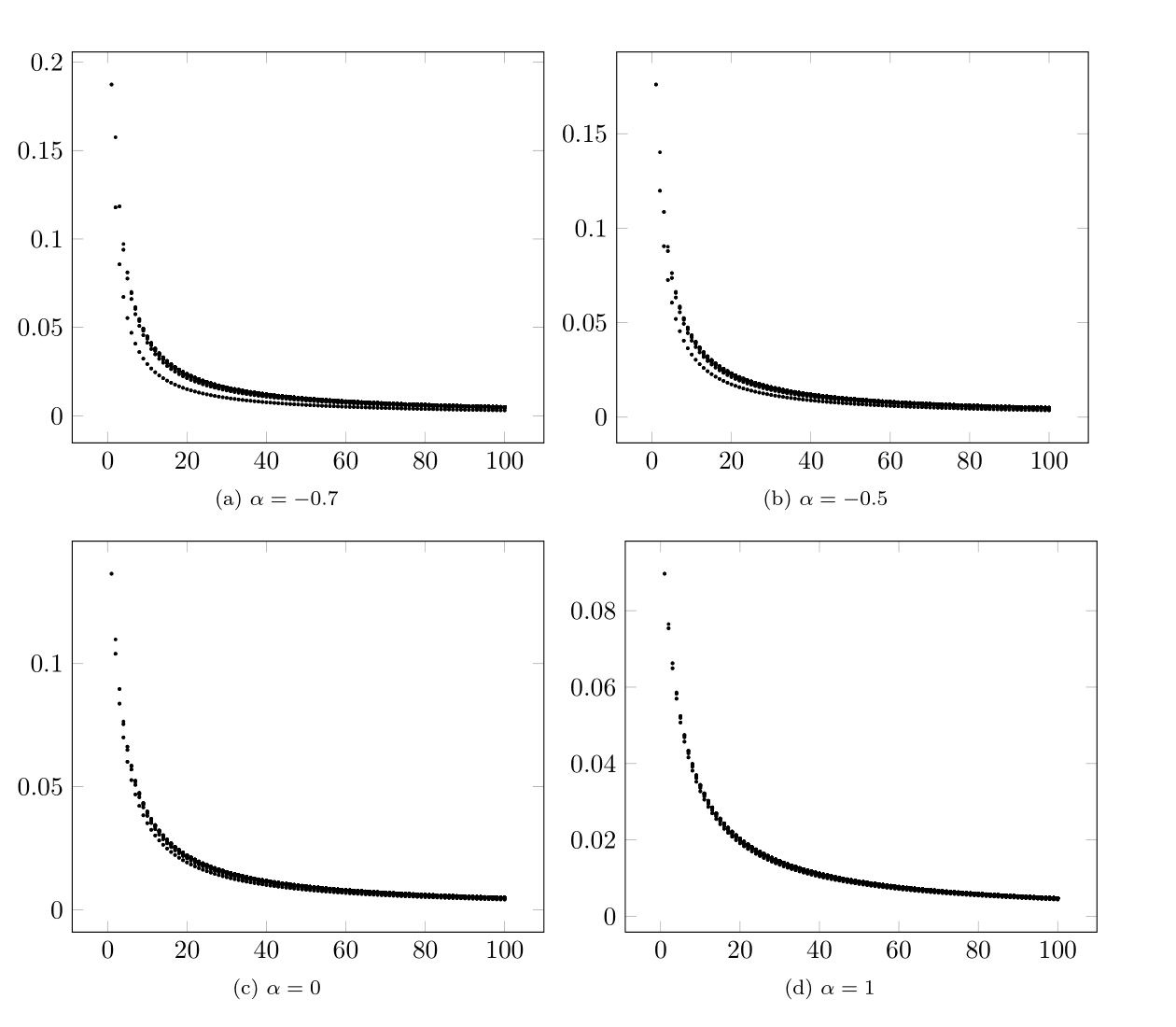
Figure 9: Expected information gain vs. $N$ for fixed $\alpha$. Y-axis is the value of expected information and X-axis is the value of $N$. All expected information gain are positive. The shapes of each graph are also very similar with few divergent lines. As $\alpha$ increasing, the divergent lines getting fewer.

We first show the numerical results of expected information gain under different priors. It is clearly that all points are above x-axis which means the expected information gain is positive-definite, which is anticipated. Since $I_{rel}$ and $\langle p\rangle$ are both positive, $\overline{I_{rel}}$ must also be positive.

As the discussions of differential information gain and relative information gain, we are also interested in the dependence of the expected information gain about $\alpha$ or $h_{N}$. However such dependence is very weak from Fig. 9 and Fig. 10. Expected information gain shows strong robustness about $\alpha$ and $h_{N}$.

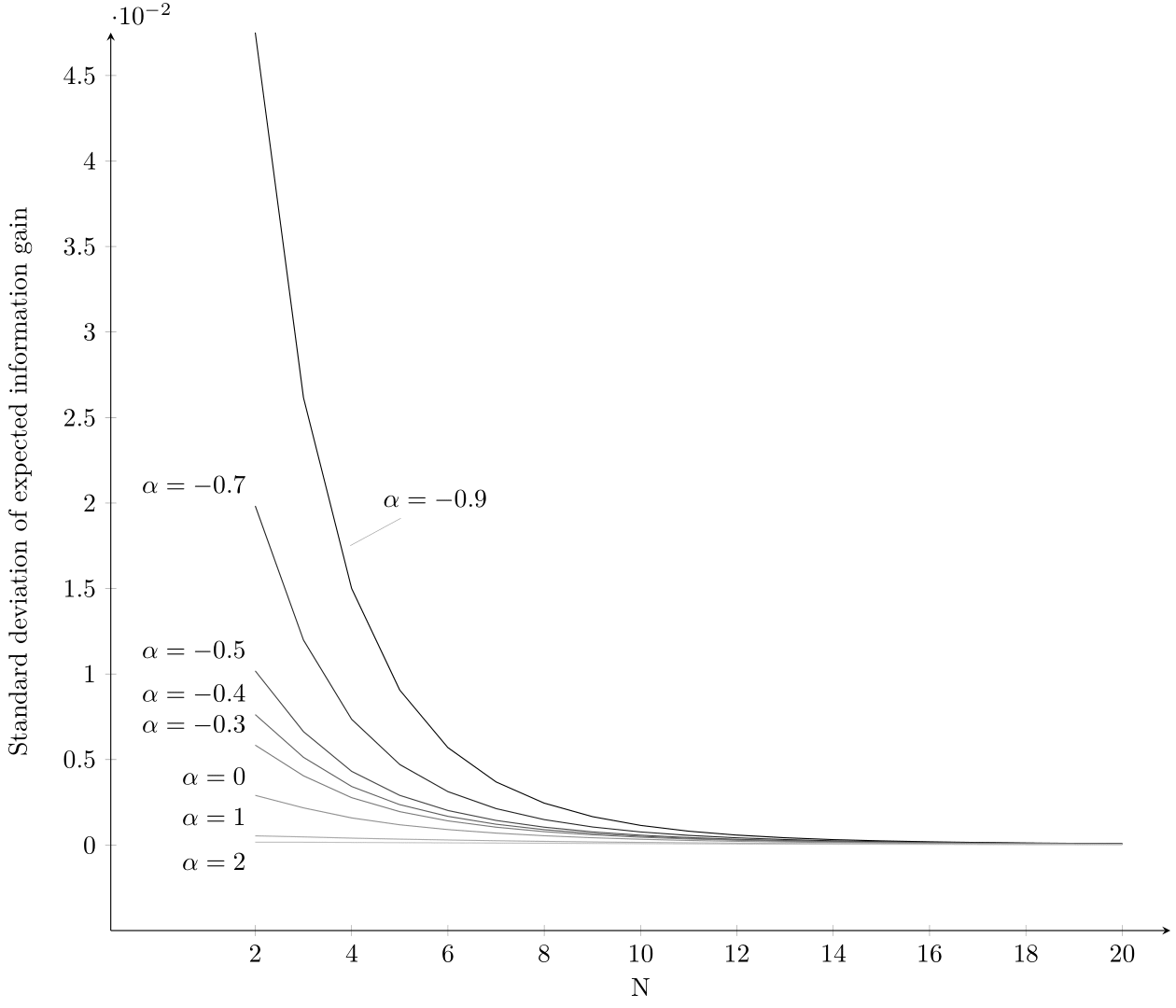
Figure 10: Robustness of expected information gain. Y-axis is the standard deviation of expected information gain over all possible $h_{N}$, X-axis is the value of $N$. As $N$ increases and even for relative very small $N$, the standard deviation tends to zero for all priors.

The asymptotic expression of expected information gain is

$$\overline{I_{diff}}=\overline{I_{rel}}=\frac{1}{2N}$$ (22)

6 Comparison of Three Information Gain and Information Increase Principle

All three measures are based on KL divergence, however, strictly speaking none of them can be a “measure” since the triangle inequality cannot be satisfied. We can still use measure to denote their role when quantifying the information gain in measurements.

From the view of operational perspective, they can be divided into two types: differential information gain and relative information gain are evaluations of a measurement that has already been taken; expected information gain is a prediction of a measurement that hasn’t been taken.

From the view of positivity, that is, will this quantity always positive? This connects with our beginning question, “will more data from measurements lead to more knowledge of a system?” For relative information gain and expected information gain the answer is yes, while differential information gain is positive only under some certain priors.

All three measures are functions of $N$, $\alpha$, $h_{N}$ which characterize size of the data sequences, prior and existing data sequence respectively. How are they sensitive to the three parameters, especially for large $N$? As we known, differential information gain is heavily influenced by all three parameters, only when $\alpha=-0.5$ differential information gain will be nearly independent of $h_{N}$. relative information gain is not sensitive to priors, in large $N$, relative information gain is affected by $h_{N}$ and $N$, while expected information gain only depends on $N$.

	Positivity	Robustness about $T_{N}$
Diff Infor. Gain	Strictly positive for all cases when $\alpha<\alpha_{p}$ where $\alpha_{p}\approxeq-0.68$. Asymptotic positive when $\alpha\leq-0.5$.	Robustness exists only when $\alpha=-0.5$ of beta distribution prior.
Rel Infor. Gain	Strictly positive for all priors.	No significant differences of robustness among beta distribution priors.
Exp. Infor. Gain	Strictly positive for all priors.	No significant differences of robustness among beta distribution priors.

Table 2: Comparison of three information gain

Initially we may hope that the idea ”more data from measurements lead to more knowledge about the system” is strictly hold, that is, the information gain of the additional data should be strictly positive under all cases. However, based on the observation of the “Black Swan Event”, we find a strictly positive information gain may not be meaningful. In the extreme case that first $N$ tosses are all tails and the $N+1$th toss is head, a negative information gain in this $N+1$th toss may be more physically reasonable. We propose the Principle of Information Gain as follows:

In a series of binomial distribution data, the information gain of the additional data should be positive asymptotically; in the extreme case that first $N$ trials of data are all the same and the data of $N+1$th trial is opposite to previous data, then the information gain in this extreme case should be negative.

Under this criterion, the differential information gain should be a better choice to measure the degree of knowledge of the additional data. The beta distribution prior may be ranged between $-0.68\lessapprox\alpha\leq-0.5$. If we also consider about the robustness of information gain over different given data, then the Jeffreys’ binomial prior ($\alpha=-0.5$) would be the best choice.

7 Related Work

7.1 Information Increase Principle and Jeffreys’ binomial prior

Summhammer [1][2] first initiates the idea that “more measurements lead to more knowledge about a physical quantity”. He quantifies the knowledge of a quantity as the uncertainty range of a quantity after a number of repeated measurements. “More measurements lead to more knowledge about a physical quantity” is interpreted as “the uncertainty range of a physical quantity should be decreasing as the number of measurements increasing”. For a quantity $\theta$, the uncertainty range $\Delta\theta$ is a function of the number of measurements

$$\Delta\theta(N+1)<\Delta\theta(N)$$ (23)

If such a quantity is determined by probability of a two-outcome measurement, say the probability of heads $p$ in coin tossing, then the uncertainty range of $\theta$ and uncertainty range of $p$ has the following relation.

$$\Delta\theta=|\frac{\partial\theta}{\partial p}|\Delta p$$ (24)

In large $N$ approximation, $\Delta p=\sqrt{\frac{p(1-p)}{N}}$. It is possible to construct the following relation to satisfy (23).

$$\Delta\theta\sqrt{N}=|\frac{\partial\theta}{\partial p}|\sqrt{p(1-p)}=constant$$ (25)

The relation between $\theta$ and $p$ yields that the prior of the probability is Jeffreys’ binomial prior under the assumption that the prior of the physical quantity is uniform distribution.

$$Pr(p|I)=|\frac{\partial\theta}{\partial p}|Pr(\theta|I)=\frac{constant}{\sqrt{p(1-p)}}$$ (26)

In the large $N$ approximation, Summhammer arrives at the the result that the prior of the associated probability of the physical quantity must be Jeffreys’ binomial prior in order to satisfy the idea that “more measurements lead to more knowledge”. Summhammer doesn’t use information theory to quantify “knowledge” about a physical quantity, but just use the range of measurement uncertainty, which is a statistical quantity. We are using the degree of uncertainty, which is the start point of information theory, to redefine the “knowledge” about a quantity, especially a probabilistic quantity. In asymptotic cases these two approaches have the same result, and we also show that why the asymptotic case is necessary.

Goyal [22] proposes the Principle of Information Gain, “In $n$ interrogations of $N$-outcome probabilistic source with unknown probabilistic vector $\vec{P}$, the amount of Shannon-Jaynes information provided by the data about $\vec{P}$ is independent of $\vec{P}$ for all $\vec{P}$ in the limit $n\rightarrow\infty$”, and proves the equivalence between this principle and Jeffreys’ rule. Under the Principle of Information Gain, the Jeffreys’ multinomial prior is derived. In the case of two-outcome probabilistic model, the Jeffreys’ multinomial prior reduces to Jeffreys’ binomial prior. The asymptotic analysis shows that the Shannon-Jaynes information is not only independent of the probability vector $\vec{P}$ but a monotonically increasing with the number of interrogations. Noticing that the Shannon-Jaynes information can be regarded as the accumulation of differential information gain. This asymptotic result also agree with our result, under Jeffreys’ binomial prior, the differential information gain is only dependent on number of measurements.

7.2 Other Information-theoretical motivation of Jeffreys’ binomial prior

Wootters [19] provides a different approach to Jeffreys’ binomial prior where quantum measurement can be used as communication channel. Alice wants to send a continuous variable, $\theta$, to Bob. Yet she doesn’t send the variable to Bob directly, instead she sends a collection of identical coins to Bob and the probability of getting heads $p(\theta)$ in each toss is a function of $\theta$. Bob tries to maximize the information of $\theta$ from a finite number of tosses. The information used here is the mutual information between $\theta$ and the number of heads $n$ in total $N$ tosses.

$$I(n:\theta)=H(n)-H(n|\theta)=-\sum_{n=0}^{N}p(n)\ln P(n)-\left\langle-\sum_{n=0}^{N}p(n|p(\theta))\ln p(n|p(\theta))\right\rangle$$ (27)

The function $p(\theta)$ is unknown and the optimization begin from a discrete values of $\{p_{1},p_{2},\cdots,p_{L}\}$ instead of using the continuous function $p(\theta)$. For each discrete value $p_{k}$, there is a weight $w_{k}$. The mutual information is now becomes:

$$I(n:\theta)=-\sum_{n=0}^{N}p(n)\ln P(n)+\sum_{k=1}^{L}w_{k}\sum_{n=0}^{N}p(n|p_{k})\ln p(n|p_{k})$$ (28)

It turns out that in the large $N$ approximation, the weight $w$ has the following form:

$$w(p)=\frac{1}{\pi\sqrt{p(1-p)}}$$ (29)

which acting like the prior probability of $p$. And this prior probability is just the Jeffreys’ binomial prior. Similar procedure can be generalized to Jeffreys’ multinomial prior distribution. Wootters’ approach is similar to the idea of reference prior, the selected prior should maximize the mutual information which is just the expected information gain over all data. The result agrees with the reference prior for multinomial data [23] and this shows another informational meaning of Jeffreys’ prior.

8 Conclusion

In this paper we investigate the concept of information gain for two-outcome quantum systems from an operational perspective. We propose an informational postulate – Principle of Information Gain – as a criterion to filter the proper measure of quantifying the amount of information gain from measurements as well as the choice of prior. It is found that the differential information gain is the most physical meaningful measure compare to another candidate, the relative information gain.

The Jeffreys’ binomial prior shows significant features in the two-outcome quantum systems. Summhammer and us shows that under this prior, the intuitive idea of ”more measurements lead to more knowledge about the physical system” is valid, from two ways of quantifying knowledge. Wootters shows that it is possible to communicate maximal information under this prior. We also show that Jeffereys’ binomial prior is (the most robust under). All these suggest the informational meaning of Jeffreys’ prior is manifold.

Currently we cannot explain the orgin of the robustness of Jeffreys’ binomial prior. It is an interesting question whether this feature could be extended to multinomial distributions or even other type probabilistic system. We guess there could be another informational intuitiveness of the robustness of Jeffreys’ prior. In this paper we mainly focus on the single parameter beta distribution prior for binomial distribution, we believe similar results will also be shown in multinomial distributions. Yet it is an open question what’s the behavior of differential information gain under a general type of priors as well as the distributions.

Appendix A Derivation of Differential Information Gain

The posterior is determined by $T_{N}$ and prior. For the sake of simplicity we would set the prior belongs to the family of beta distributions:

$$Pr(p|I)=\frac{p^{\alpha}(1-p)^{\alpha}}{B(\alpha+1,\alpha+1)}$$ (30)

where $\alpha>-1,B(x,y)$ is the beta function.

Given $N$, there are $2^{N}$ different $T_{N}$. However, we may not need to calculate all the $2^{N}$ sequences. Suppose every toss is independent, this happens in quantum mechanics, then this coin tossing model would become a binomial distribution. Let $h_{N}$ be the number of heads inside $T_{N}$, the posterior $Pr(p|N,T_{N},I)$ is equivalent to $Pr(p|N,h_{N},I)$ and likelihood will be

$$Pr(h_{N}|N,p,I)={{N}\choose{h_{N}}}p^{h_{N}}(1-p)^{N-h_{N}}$$ (31)

hence the posterior after $N$ tosses

$$Pr(p|N,h_{N},I) =\frac{Pr(h_{N}|N,p,I)Pr(p|I)}{\int Pr(h_{N}|N,p,I)Pr(p|I)dp}$$ (32)

$$=\frac{p^{h_{N}+\alpha}(1-p)^{N-h_{N}+\alpha}}{B(h_{N}+\alpha+1,N-h_{N}+\alpha+1)}$$

The information gain in the $N+1$th toss would be

$$I_{diff}=D_{KL}(Pr(p|N+1,\{T_{N},t_{N+1}\},I)||Pr(p|I))-D_{KL}(Pr(p|N,h_{N},I)||Pr(p|I))$$ (33)

$I_{diff}$ is determined by $h_{N}$, prior and the result of $N+1$th toss $t_{N+1}$. $t_{N+1}$ could be either “Head” or “Tail”, then posterior after $N+1$ tosses could be

$$Pr(p|N+1,\{T_{N},t_{N+1}=``Head"\},I)=\frac{p^{h_{N}+\alpha+1}(1-p)^{N-h_{N}+\alpha}}{B(h_{N}+\alpha+2,N-h_{N}+\alpha+1)}$$ (34)

$$Pr(p|N+1,\{T_{N},t_{N+1}=``Tail"\},I)=\frac{p^{h_{N}+\alpha}(1-p)^{N-h_{N}+\alpha+1}}{B(h_{N}+\alpha+1,N-h_{N}+\alpha+2)}$$ (35)

Taking $t_{N+1}=``Head"$,the first term in (33) would become

$$D_{KL}(Pr(p|N+1,\{T_{N},t_{N+1}=``Head"\},I)||Pr(p|I))$$ (36)

$$=\int_{0}^{1}Pr(p|N+1,h_{N}+1,I)ln[\frac{Pr(p|N+1,h_{N}+1,I)}{Pr(p|I)}]dp$$

$$=\int_{0}^{1}\frac{p^{h_{N}+\alpha+1}(1-p)^{N-h_{N}+\alpha}}{B(h_{N}+\alpha+2,N-h_{N}+\alpha+1)}ln[\frac{p^{h_{N}+1}(1-p)^{N-h_{N}}B(\alpha+1,\alpha+1)}{B(h_{N}+\alpha+2,N-h_{N}+\alpha+1)}]dp$$

$$=\int_{0}^{1}\frac{p^{h_{N}+\alpha+1}(1-p)^{N-h_{N}+\alpha}}{B(h_{N}+\alpha+2,N-h_{N}+\alpha+1)}\{ln[p^{h_{N}+1}(1-p)^{N-h_{N}}]+ln[\frac{B(\alpha+1,\alpha+1)}{B(h_{N}+\alpha+2,N-h_{N}+\alpha+1)}]\}dp$$

$$=\int_{0}^{1}\frac{p^{h_{N}+\alpha+1}(1-p)^{n-h_{N}+\alpha}}{B(h_{N}+\alpha+1,n-h_{N}+\alpha+1)}ln[p^{h_{N}+1}(1-p)^{N-h_{N}}]dp+ln[\frac{B(\alpha+1,\alpha+1)}{B(h_{N}+\alpha+2,n-h_{N}+\alpha+1)}]$$

By using the integral

$$\int_{0}^{1}x^{a}(1-x)^{b}ln(x)dx=B(a+1,b+1)[\psi(a+1)-\psi(a+b+2)]$$ (37)

where $\psi(x)$ is the digamma function, we can obtain the following result

$$D_{KL}(Pr(p|N+1,\{T_{N},t_{N+1}=``Head"\},I)||Pr(p|I))= (h_{N}+1)\psi(h_{N}+\alpha+2)+(N-h_{N})\psi(N-h_{N}+\alpha+1)$$ (38)

$$-(N+1)\psi(N+2\alpha+3)$$

$$+ln[\frac{B(\alpha+1,\alpha+1)}{B(h_{N}+\alpha+2,n-h_{N}+\alpha+1)}]$$

The second term in (33) would become

$$D_{KL}(Pr(p|N,h_{N},I)||Pr(p|I))$$ (39)

$$=\int_{0}^{1}Pr(p|N,h_{N},I)ln[\frac{Pr(p|N,h_{N},I)}{Pr(p|I)}]dp$$

$$=\int_{0}^{1}\frac{p^{h_{N}+\alpha}(1-p)^{N-h_{N}+\alpha}}{B(h_{N}+\alpha+1,N-h_{N}+\alpha+1)}ln[\frac{p^{h_{N}}(1-p)^{N-h_{N}}B(\alpha+1,\alpha+1)}{B(h_{N}+\alpha+1,N-h_{N}+\alpha+1)}]dp$$

$$=\int_{0}^{1}\frac{p^{h_{N}+\alpha}(1-p)^{N-h_{N}+\alpha}}{B(h_{N}+\alpha+1,N-h_{N}+\alpha+1)}\{ln[p^{h_{N}}(1-p)^{N-h_{N}}]+ln[\frac{B(\alpha+1,\alpha+1)}{B(h_{N}+\alpha+1,N-h_{N}+\alpha+1)}]\}dp$$

$$=\int_{0}^{1}\frac{p^{h_{N}+\alpha}(1-p)^{n-h_{N}+\alpha}}{B(h_{N}+\alpha+1,n-h_{N}+\alpha+1)}ln[p^{h_{N}}(1-p)^{N-h_{N}}]dp+ln\frac{B(\alpha+1,\alpha+1)}{B(h_{N}+\alpha+1,n-h_{N}+\alpha+1)}$$

$$=h_{N}\psi(h_{N}+\alpha+1)+(N-h_{N})\psi(N-h_{N}+\alpha+1)-N\psi(N+2\alpha+2)+ln[\frac{B(\alpha+1,\alpha+1)}{B(h_{N}+\alpha+1,n-h_{N}+\alpha+1)}]$$

Now we obtain the final expression of (33)

$$I_{diff}(t_{N+1}=``Head")= ~{}D_{KL}(Pr(p|N+1,\{T_{N},t_{N+1}=``Head"\},I)||Pr(p|I))-D_{KL}(Pr(p|N,h_{N},I)||Pr(p|I))$$ (40)

$$= ~{}\psi(h_{N}+\alpha+2)-\psi(N+2\alpha+3)+$$

$$\frac{h_{N}}{h_{N}+\alpha+1}-\frac{N}{N+2\alpha+2}+\ln{\frac{N+2\alpha+2}{h_{N}+\alpha+1}}$$

Similarly we can obtain the $I_{diff}$ when $t_{N+1}=``Tail"$

$$I_{diff}(t_{N+1}=``Tail")= ~{}\psi(N-h_{N}+\alpha+2)-\psi(N-h_{N}+2\alpha+3)+$$ (41)

$$~{}\frac{N-h_{N}}{N-h_{N}+\alpha+1}-\frac{N}{N+2\alpha+2}+\ln{\frac{N+2\alpha+2}{N-h_{N}+\alpha+1}}$$

This suggests that for fixed $N$ and $\alpha$, $I_{diff}(t_{N+1}=``Head")$ and $I_{diff}(t_{N+1}=``Tail")$ are symmetric since $h_{N}$ is ranging from $0$ to $N$.

Appendix B Derivation of Relative Information Gain

From Appendix A we know that the posterior after $N$ tosses is

$$Pr(p|N,T_{N},I)=Pr(p|N,h_{N},I)=\frac{p^{h_{N}+\alpha}(1-p)^{N-h_{N}+\alpha}}{B(h_{N}+\alpha+1,N-h_{N}+\alpha+1)}$$ (42)

Therefore the posterior after $N+1$ tosses would be

$$Pr(p|N+1,T_{N+1},I)=\frac{Pr(h_{N},T_{N+1}|p,N+1,I)Pr(p|I)}{\int_{0}^{1}Pr(h_{N},T_{N+1}|p,N+1,I)Pr(p|I)dp}$$ (43)

Depends on different results of $t_{N+1}$, the posterior after $N+1$ tosses would be

$$Pr(p|N+1,\{T_{N},t_{N+1}=``Head"\},I)=\frac{p^{h_{N}+\alpha+1}(1-p)^{N-h_{N}+\alpha}}{B(h_{N}+\alpha+2,N-h_{N}+\alpha+1)}$$ (44)

$$Pr(p|N+1,\{T_{N},t_{N+1}=``Tail"\},I)=\frac{p^{h_{N}+\alpha}(1-p)^{N-h_{N}+\alpha+1}}{B(h_{N}+\alpha+1,N-h_{N}+\alpha+2)}$$ (45)

And the corresponding relative information gain would be

$$I_{rel}(t_{N+1}=``Head")$$ (46)

$$=D_{KL}(Pr(p|N+1,\{T_{N},t_{N+1}=``Head"\},I)||Pr(p|N,h_{N},I))$$

$$=\int_{0}^{1}Pr(p|N+1,\{T_{N},t_{N+1}=``Head"\},I)\ln{\frac{Pr(p|N+1,\{T_{N},t_{N+1}=``Head"\},I)}{Pr(p|N,h_{N},I)}}dp$$

$$=\int_{0}^{1}\frac{p^{h_{N}+\alpha+1}(1-p)^{N-h_{N}+\alpha}}{B(h_{N}+\alpha+2,N-h_{N}+\alpha+1)}\ln{\frac{pB(h_{N}+\alpha+1,N-h_{N}+\alpha+1)}{B(h_{N}+\alpha+2,N-h_{N}+\alpha+1)}}dp$$

$$=\psi(h_{N}+\alpha+2)-\psi(N+2\alpha+3)+\ln{\frac{N+2\alpha+2}{h_{N}+\alpha+1}}$$

$$I_{rel}(t_{N+1}=``Tail")=\psi(N-h_{N}+\alpha+2)-\psi(N-h_{N}+2\alpha+3)+\ln{\frac{N+2\alpha+2}{N-h_{N}+\alpha+1}}$$ (47)

Appendix C Equivalence of Expected Differential Information Gain and Expected Relative Information Gain

From  (19), we know

$$\langle p\rangle=\int_{0}^{1}p~{}Pr(p|N,h_{N},I)~{}dp$$ (48)

If the $N+1$th toss is “Head”, then the posterior after $N+1$ tosses can be written as

$$Pr(p|N+1,\{T_{N},t_{N+1}=``Head"\},I)=\frac{p~{}Pr(p|N,h_{N},I)}{\int_{0}^{1}p~{}Pr(p|N,h_{N},I)~{}dp}=\frac{p~{}Pr(p|N,h_{N},I)}{\langle p\rangle}$$ (49)

Then we can rewrite $I_{diff}$ as

$$I_{diff}(t_{N+1}=``Head")= D_{KL}(Pr(p|N+1,\{T_{N},t_{N+1}=``Head"\},I)||Pr(p|I))-D_{KL}(Pr(p|N,h_{N},I)||Pr(P|I))$$ (50)

$$= \int_{0}^{1}\frac{p~{}Pr(p|N,h_{N},I)}{\langle p\rangle}\ln{\frac{p~{}Pr(p|N,h_{N},I)}{\langle p\rangle~{}Pr(p|I)}}~{}dp-\int_{0}^{1}Pr(p|N,h_{N},I)\ln{\frac{Pr(p|N,h_{N},I)}{Pr(p|I)}}~{}dp$$

$$= \int_{0}^{1}\frac{p~{}Pr(p|N,h_{N},I)}{\langle p\rangle}\left(\ln{\frac{Pr(p|N,h_{N},I)}{Pr(p|I)}}+\ln{\frac{p}{\langle p\rangle}}\right)~{}dp$$

$$-\int_{0}^{1}Pr(p|N,h_{N},I)\ln{\frac{Pr(p|N,h_{N},I)}{Pr(p|I)}}~{}dp$$

Similarly if $t_{N+1}=``Tail"$,

$$I_{diff}(t_{N+1}=``Tail")= D_{KL}(Pr(p|N+1,\{T_{N},t_{N+1}=``Tail"\},I)||Pr(p|I))-D_{KL}(Pr(p|N,h_{N},I)||Pr(p|I))$$ (51)

$$= \int_{0}^{1}\frac{(1-p)~{}Pr(p|N,h_{N},I)}{\langle 1-p\rangle}\left(\ln{\frac{Pr(p|N,h_{N},I)}{Pr(p|I)}}+\ln{\frac{1-p}{\langle 1-p\rangle}}\right)~{}dp$$

$$-\int_{0}^{1}Pr(p|N,h_{N},I)\ln{\frac{Pr(p|N,h_{N},I)}{Pr(p|I)}}~{}dp$$

Then the expected differential information gain would be

$$\overline{I_{diff}}= \langle p\rangle\times I_{diff}(t_{N+1}=``Head")+\langle 1-p\rangle\times I_{diff}(t_{N+1}=``Tail")$$ (52)

$$= \int_{0}^{1}p~{}Pr(p|N,h_{N},I)\left(\ln{\frac{Pr(p|N,h_{N},I)}{Pr(p|I)}}+\ln{\frac{p}{\langle p\rangle}}\right)~{}dp$$

$$+\int_{0}^{1}(1-p)~{}Pr(p|N,h_{N},I)\left(\ln{\frac{Pr(p|N,h_{N},I)}{Pr(p|I)}}+\ln{\frac{1-p}{\langle 1-p\rangle}}\right)~{}dp$$

$$-\int_{0}^{1}Pr(p|N,h_{N},I)\ln{\frac{Pr(p|N,h_{N},I)}{Pr(p|I)}}~{}dp$$

$$= \int_{0}^{1}Pr(p|N,h_{N},I)\left(p~{}\ln{\frac{p}{\langle p\rangle}}+(1-p)~{}\ln{\frac{1-p}{\langle 1-p\rangle}}\right)~{}dp$$

Similarly, $I_{rel}$ can be written as

$$I_{rel}(t_{N+1}=``Head") =D_{KL}(Pr(p|N+1,\{T_{N},t_{N+1}=``Head"\},I)||Pr(p|N,h_{N},I))$$ (53)

$$=\int_{0}^{1}\frac{p~{}Pr(p|N,h_{N},I)}{\langle p\rangle}\ln{\frac{p}{\langle p\rangle}}~{}dp$$

$$I_{rel}(t_{N+1}=``Tail") =D_{KL}(Pr(p|N+1,\{T_{N},t_{N+1}=``Tail"\},I)||Pr(p|N,h_{N},I))$$ (54)

$$=\int_{0}^{1}\frac{(1-p)~{}Pr(p|N,h_{N},I)}{\langle 1-p\rangle}\ln{\frac{1-p}{\langle 1-p\rangle}}~{}dp$$

Then the expected relative information gain would be

$$\overline{I_{rel}} =\langle p\rangle\times I_{rel}(t_{N+1}=``Head")+\langle 1-p\rangle\times I_{rel}(t_{N+1}=``Tail")$$ (55)

$$=\int_{0}^{1}p~{}Pr(p|N,h_{N},I)~{}\ln{\frac{p}{\langle p\rangle}}~{}dp+\int_{0}^{1}(1-p)~{}Pr(p|N,h_{N},I)~{}\ln{\frac{1-p}{\langle 1-p\rangle}}~{}dp$$

$$=\int_{0}^{1}Pr(p|N,h_{N},I)\left(p~{}\ln{\frac{p}{\langle p\rangle}}+(1-p)~{}\ln{\frac{1-p}{\langle 1-p\rangle}}\right)~{}dp$$

From (52) and (55) we may see that in this two-outcome model, the expected differential information gain $\overline{I_{diff}}$ and expected relative information gain $\overline{I_{rel}}$ are equal under all kinds of priors.

References

- [1] Johann Summhammer. Maximum predictive power and the superposition principle. International Journal of Theoretical Physics, 33:171–178, 1994.
- [2] Johann Summhammer. Maximum predictive power and the superposition principle, 1999.
- [3] M K Patra. Quantum state determination: estimates for information gain and some exact calculations. Journal of Physics A: Mathematical and Theoretical, 40(35):10887–10902, aug 2007.
- [4] Vaibhav Madhok, Carlos A. Riofrío, Shohini Ghose, and Ivan H. Deutsch. Information gain in tomography–a quantum signature of chaos. Physical Review Letters, 112:014102, Jan 2014.
- [5] Hui Khoon Ng Yihui Quek, Stanislav Fort. Adaptive quantum state tomography with neural networks. npj Quantum Information, 7(105), 2021.
- [6] Rishabh Gupta, Rongxin Xia, Raphael D. Levine, and Sabre Kais. Maximal entropy approach for quantum state tomography. PRX Quantum, 2:010318, Feb 2021.
- [7] Robert D. McMichael, Sergey Dushenko, and Sean M. Blakley. Sequential bayesian experiment design for adaptive ramsey sequence measurements. Journal of Applied Physics, 130(14):144401, 2021.
- [8] Ben Placek, Daniel Angerhausen, and Kevin H. Knuth. Analyzing exoplanet phase curve information content: Toward optimized observing strategies. The Astronomical Journal, 154(4):154, sep 2017.
- [9] Chun-Wang Ma and Yu-Gang Ma. Shannon information entropy in heavy-ion collisions. Progress in Particle and Nuclear Physics, 99:120–158, 2018.
- [10] Č. Brukner and A. Zeilinger. Information invariance and quantum probabilities. Foundations of Physics, 39:677–689, July 2009.
- [11] Philip Goyal. Information-geometric reconstruction of quantum theory. Phys. Rev. A, 78:052120, Nov 2008.
- [12] Ariel Caticha. Entropic dynamics, time and quantum theory. Journal of Physics A: Mathematical and Theoretical, 44(22):225303, may 2011.
- [13] Lluís Masanes, Markus P. Müller, Remigiusz Augusiak, and David Pérez-García. Existence of an information unit as a postulate of quantum theory. Proceedings of the National Academy of Sciences, 110(41):16373–16377, 2013.
- [14] H. De Raedt, M. I. Katsnelson, and K. Michielsen. Quantum theory as plausible reasoning applied to data obtained by robust experiments. Philosophical Transactions of the Royal Society A: Mathematical, Physical and Engineering Sciences, 374(2068):20150233, 2016.
- [15] Philipp Andres Höhn. Quantum theory from rules on information acquisition. Entropy, 19(3), 2017.
- [16] S Aravinda, R Srikanth, and Anirban Pathak. On the origin of nonclassicality in single systems. Journal of Physics A: Mathematical and Theoretical, 50(46):465303, oct 2017.
- [17] L. Czekaj, M. Horodecki, P. Horodecki, and R. Horodecki. Information content of systems as a physical principle. Phys. Rev. A, 95:022119, Feb 2017.
- [18] Giulio Chiribella. Agents, subsystems, and the conservation of information. Entropy, 20(5), 2018.
- [19] William K. Wootters. Communicating through probabilities: Does quantum theoryoptimize the transfer of information? Entropy, 15(8):3130–3147, 2013.
- [20] Thomas M. Cover; Joy A. Thomas. Differential Entropy, chapter 8, pages 243–259. John Wiley & Sons, Ltd, 2005.
- [21] E. T. Jaynes. Information Theory and Statistical Mechanics, pages 181–218. W. A. Benjamin, Inc., 1963.
- [22] Philip Goyal. Prior probabilities: An information‐theoretic approach. AIP Conference Proceedings, 803(1):366–373, 2005.
- [23] James O. Berger and Jose M. Bernardo. Ordered group reference priors with application to the multinomial problem. Biometrika, 79(1):25–37, 1992.