Discontinuous Galerkin methods for a first-order semi-linear hyperbolic continuum model of a topological resonator dimer array

Qiang Du Department of Applied Physics and Applied Mathematics, Columbia University, New York, NY 10027, USA. Email: qd2125@columbia.edu    Huaiyu Li Department of Applied Physics and Applied Mathematics, Columbia University, New York, NY 10027, USA. Email: hl3002@columbia.edu    Michael Weinstein Department of Applied Physics and Applied Mathematics, Columbia University, New York, NY 10027, USA. Email: miw2103@columbia.edu    Lu Zhang Department of Applied Physics and Applied Mathematics, Columbia University, New York, NY 10027, USA. Email: lz2784@columbia.edu

Abstract

We present discontinuous Galerkin (DG) methods for solving a first-order semi-linear hyperbolic system, which was originally proposed as a continuum model for a one-dimensional dimer lattice of topological resonators. We examine the energy-conserving or energy-dissipating property in relation to the choices of simple, mesh-independent numerical fluxes. We demonstrate that, with certain numerical flux choices, our DG method achieves optimal convergence in the $L^{2}$ norm. We provide numerical experiments that validate and illustrate the effectiveness of our proposed numerical methods

Keywords: discontinuous Galerkin, first-order hyperbolic system, stability, error estimates, topological resonators, dynamics of coherent structure AMS subject: 65M12, 65M60, 35L40, 35C07, 78A40

1 Introduction

There is great interest in the robust transport of energy in naturally occurring and engineered materials. A very active direction is the field of topological materials, which emerged from the recognition that materials with topologically nontrivial (Floquet) band structure when perturbed, for example, by extended defects (domain walls, terminated along line defects,…), support robust edge (interface) states whose properties are stable against large but localized perturbations of the system. The role of band structure topology in wave physics was first recognized in the context of condensed matter physics, e.g., the integer quantum Hall effect [32], and topological insulators [26].

There is very wide interest in technologies based on topologically protected states due to the potential for extraordinarily robust energy and information transfer in communications and computing. This has motivated the exploration of topological wave phenomena observed in engineered metamaterial systems in photonics, acoustics, electronics, elasticity, and mechanics [25, 51, 40, 37, 38, 23, 4, 29] which, in the regime of linear phenomena, are characterized by a linear band structure. A simple discrete model, which has been very influential, is the dimer model emerging from the work of Su-Schrieffer-Heeger (SSH) [27, 49] on the Peierls instability. Such systems can naturally be probed in the nonlinear regime via strong excitation. So it is of great interest to study whether topological properties persist in the regime where nonlinear effects are present and whether perhaps different topological phenomena emerge [24, 5, 6, 30, 46].

With a view toward exploring topologically protected states in the nonlinear systems, Haddad, Vitelli, and Alu (HVA) [23, 47] introduced a discrete and nonlinear variant of SSH, modeling a spatially periodic nonlinear dimer array of electrical circuits. In each period cell of the array are two nonlinear circuit oscillators, and cells are linearly coupled to their nearest neighbors. Numerical simulations in the propagation of traveling kink-like and pulse-like states. The formal continuum of the limit of the HVA discrete system is a coupled system of first-order semi-linear hyperbolic partial differential equations. After scaling, the system can be written in the form:

$$\partial_{t}b_{1} =\partial_{x}b_{2}+N\left(b_{1},b_{2}\right)b_{2},$$ (1.1)

$$\partial_{t}b_{2} =\partial_{x}b_{1}-N\left(b_{1},b_{2}\right)b_{1}.$$

Here, $b_{1}(x,t)$ and $b_{2}(x,t)$ are continuum limits of field amplitudes (which modulate a $\pi-$ quasimomentum Bloch modes of the underlying SSH model) at time $t$ for the two nonlinearly coupled circuits in the dimer at location $x$. After appropriate normalization, the nonlinearity can be taken of the form: $N(b_{1},b_{2})=N(\sqrt{b_{1}^{2}+b_{2}^{2}})$ and such that

$$N(0)=1,\quad N(1)=0,\ N^{\prime}(r)<0,\quad N(r)\to N_{\infty}<0\ \textrm{as}\ r\to+\infty.$$ (1.2)

The continuum model is shown to have a rich family of traveling wave solutions (TWSs): subsonic (speed $|c|<1$) and supersonic (speed $|c|>1$) pulses, and subsonic kinks. Here, $|c|=1$ is the maximum group speed of linearized perturbation against spatially-uniform equilibria. The exponential stability of supersonic pulses in an appropriate weighted function space is established in [36]; dark soliton-like supersonic pulses always outrun any compactly supported perturbations, however large. Subsonic pulses are exponentially unstable. The linearized analysis of [36] shows that kinks with cubic nonlinearity are linearly neutrally stable. Hence its nonlinear dynamics are far more subtle. To investigate the nonlinear stability properties of kinks, we desire a stable and efficient scheme for the evolution of data initialized near kinks.

In this work, we devote our effort to the numerical studies of the semi-linear hyperbolic system (1.1). For such systems, there is plenty of literature on the numerical approximation, such as finite difference method [48, 3], finite volume method [35, 20], finite element method [33, 14], spectral method [22, 50], and particle method [21, 42]. Here, we focus on discontinuous Galerkin (DG) methods. DG method is a class of finite element methods using discontinuous piecewise polynomials for numerical solutions and test functions in spatial variables. The first DG method was introduced in $1973$ by Reed and Hill for the neutron transport equation [43]. In the following year, Lasaint and Raviart [34] conducted the first systematic analysis of the proposed DG method and showed that the order of convergence in the $L^{2}$ norm is $q$ when using $q$-th order discontinuous finite element spaces. Later, Johnson, Nävert, and Pitkäranta improved the analysis and proved an optimal error estimate, $q+\frac{1}{2}$, in the $L^{2}$ norm [31]. Peterson [41] further showed that this error estimate is optimal and cannot be improved within the class of quasi-uniform meshes. In the late 90s, Cockburn and Shu proposed a class of total variation bounded DG methods for conservation laws [16, 15, 13, 11, 18]. Since the entropy satisfies the conditions on the numerical fluxes, these schemes are generally entropy stable. In [7, 8], Chung and Engquist analyzed an energy-conserving mixed DG method with staggered grids for first-order acoustic wave equations. With different meshes for different variables, they obtained optimal error estimates even with unstructured meshes. We refer to [12, 45] and reference therein for the development and survey of DG methods. Over the past few decades, DG methods have proven to be very efficient when solving first-order hyperbolic and nearly hyperbolic systems. Because of their attractive properties, such as arbitrary high-order accuracy, local time evolution, element-wise conservation, geometrical flexibility, hp-adaptivity, etc., they have been widely used to solve problems in many fields of science, engineering, and industry, such as computational fluid dynamics, computational acoustics, and computational magneto-hydrodynamics, see [10, 39, 44] and reference therein. While the system under consideration is new and involves special nonlinear couplings, it is of a hyperbolic/wave nature. The development of DG approximations is a natural choice for its numerical solution. It is well known that high-order methods have less dispersion and dissipation errors than their low-order counterparts, making them more favorable when simulating waves.

In this paper, we consider the first-order hyperbolic system with a nonlinear term satisfying the condition (1.2) and its spatial DG discretization to the system (2.2). After first transforming the system into one represented by the characteristic variables, it is easy to identify the direction of wave propagation on the one hand and intuitive to define numerical fluxes by following the idea of DG methods for hyperbolic equations on the other. With proper boundary conditions, the proposed semi-discrete scheme is energy-conserving or energy-dissipating, depending on the choices of simple, mesh-independent numerical fluxes. In addition, the proposed DG scheme admits optimal error estimates in the $L^{2}$ norm for suitably defined numerical fluxes. Moreover, numerical experiments show that high-order DG methods perform well in capturing the dynamic behaviors of the solutions compared to low-order methods, making the algorithmic development a promising tool to help further investigate the mathematical properties of the system and related physical phenomena.

The rest of this paper is organized as follows: Section 2 presents the governing continuum model and its conservation property. Section 4 introduces the DG semi-discretization along with several interelement fluxes and proves the basic energy estimate. In Section 5, we prove an optimal error estimate in the $L^{2}$ norm with particular numerical fluxes and present several numerical experiments to verify our theoretical findings in Section 6. Last, we summarize our results in Section 7 and point out potential areas for future research.

2 The continuum model

In this section, we introduce a first-order hyperbolic system for a pair of re-scaled variables in (1.1) with a general nonlinear coupling term $N(\cdot,\cdot)$ satisfying the condition (1.2). A key conservation property is also presented.

2.1 Model in characteristic variables and conservation property

To make the system (1.1) more amendable to mature techniques for hyperbolic equations when designing DG schemes for the system (1.1), we introduce the characteristic variables

$$\begin{pmatrix}w_{1}\\ w_{2}\end{pmatrix}=A\begin{pmatrix}b_{1}\\ b_{2}\end{pmatrix},\quad A=\frac{1}{\sqrt{2}}\begin{pmatrix}1&1\\ 1&-1\end{pmatrix}$$ (2.1)

to yield the following first-order hyperbolic system

$$\partial_{t}w_{1} =\ \ \partial_{x}w_{1}-N\left(w_{1},w_{2}\right)w_{2},\quad(x,t)\in\mathbb{R}\times(0,T),$$ (2.2)

$$\partial_{t}w_{2} =-\partial_{x}w_{2}+N\left(w_{1},w_{2}\right)w_{1},\quad(x,t)\in\mathbb{R}\times(0,T),$$

where $N(w_{1},w_{2})=N\Big{(}\frac{1}{\sqrt{2}}(w_{1}+w_{2}),\frac{1}{\sqrt{2}}(w_{1}-w_{2})\Big{)}$ retains its form as before, and the constant $T\in(0,+\infty)$ denotes the terminal time of interests.

Multiplying the first equation in (2.2) by $w_{1}$, and the second equation in (2.2) by $w_{2}$, then integrating the resulting two equations over $\mathbb{R}$ yields

$$\int_{\mathbb{R}}w_{1}\partial_{t}w_{1}\ dx =\ \ \int_{\mathbb{R}}\big{(}w_{1}\partial_{x}w_{1}-N\left(w_{1},w_{2}\right)w_{2}w_{1}\big{)}\ dx,$$ (2.3)

$$\int_{\mathbb{R}}w_{2}\partial_{t}w_{2}\ dx =-\int_{\mathbb{R}}\big{(}w_{2}\partial_{x}w_{2}-N\left(w_{1},w_{2}\right)w_{1}w_{2}\big{)}\ dx.$$ (2.4)

Next, define the energy quantity

$$E(t)=\int_{\mathbb{R}}(w_{1}^{2}+w_{2}^{2})\ dx,$$ (2.5)

and add (2.3)–(2.4) together, we obtain

$$\frac{1}{2}\frac{dE}{dt}=\frac{1}{2}\frac{d}{dt}\int_{\mathbb{R}}(w_{1}^{2}+w_{2}^{2})\ dx=\frac{1}{2}\left(w_{1}^{2}(+\infty,t)-w_{1}^{2}(-\infty,t)-w_{2}^{2}(+\infty,t)+w_{2}^{2}(-\infty,t)\right).$$ (2.6)

Given the boundary conditions that $b_{1}(x,t),b_{2}(x,t)$ decay to some constants at $x=\pm\infty$, it is clear that $w_{1}(x,t),w_{2}(x,t)$ also decay to some constants. Moreover, if $b_{1},b_{2}$ satisfy

$$b_{1}(+\infty,t)b_{2}(+\infty,t)-b_{1}(-\infty,t)b_{2}(-\infty,t)=0,$$

we then have

$$w_{1}^{2}(+\infty,t)-w_{1}^{2}(-\infty,t)-w_{2}^{2}(+\infty,t)+w_{2}^{2}(-\infty,t)=0,$$ (2.7)

namely, $\frac{d}{dt}\int_{\mathbb{R}}(w_{1}^{2}+w_{2}^{2})\ dx=0$, which implies $E(t)=E(0)$.

3 Finite speed of propagation

Now, for a given interval $(a,b)$ with $b>a$, for $t<\frac{b-a}{2}$, we define

$$E_{(a,b)}(t)=\int_{a+t}^{b-t}(w_{1}^{2}(x,t)+w_{2}^{2}(x,t))\ dx.$$ (3.1)

Then using the PDE system, we get

$$\frac{d}{dt}E_{(a,b)}(t) = 2\int_{a+t}^{b-t}(w_{1}\partial_{t}w_{1}+w_{2}\partial_{t}w_{2})\ dx-w_{1}^{2}(b-t,t)-w_{2}^{2}(b-t,t)$$

$$\qquad-w_{1}^{2}(a+t,t)-w_{2}^{2}(a+t,t)$$

$$= 2\int_{a+t}^{b-t}(w_{1}\partial_{x}w_{1}-N\left(w_{1},w_{2}\right)w_{1}w_{2}-w_{2}\partial_{x}w_{2}+N\left(w_{1},w_{2}\right)w_{2}w_{1})\ dx$$

$$\qquad-w_{1}^{2}(b-t,t)-w_{2}^{2}(b-t,t)-w_{1}^{2}(a+t,t)-w_{2}^{2}(a+t,t)$$

$$= w_{1}^{2}(b-t,t)-w_{1}^{2}(a+t,t)-w_{2}^{2}(b-t,t)+w_{2}^{2}(a+t,t)$$

$$\qquad-w_{1}^{2}(b-t,t)-w_{2}^{2}(b-t,t)-w_{1}^{2}(a+t,t)-w_{2}^{2}(a+t,t)$$

$$= -2w_{1}^{2}(a+t,t)-2w_{2}^{2}(b-t,t)\leq 0.$$

This implies

$$E_{(a,b)}(t)\leq E_{(a,b)}(0)=\int_{a}^{b}(w_{1}^{2}(x,0)+w_{2}^{2}(x,0))\ dx.$$

Thus, for initial data with compact support in $(-A,A)$, we see that the solution also has compact support $(-A-t,A+t)$ at any finite time $t$, which leads to the finite speed of propagation.

One can apply a similar argument to perturbed solutions (with the help of the uniform Liphshitz continuity of the nonlinear term and the Gronwall inequality).

4 Semi-discrete DG formulation

To derive a DG formulation for the system (2.2), we first truncate the real line to a bounded interval $[x_{a},x_{b}]\subseteq\mathbb{R}$, then discretize the computational domain $I:=[x_{a},x_{b}]\subseteq\mathbb{R}$ by non-overlapping elements $I_{j}$ such that $[x_{a},x_{b}]=\cup_{j=1}^{N}[x_{j-\frac{1}{2}},x_{j+\frac{1}{2}}]$ with $I_{j}=(x_{j-\frac{1}{2}},x_{j+\frac{1}{2}})$. In addition, denote $h_{j}:=x_{j+\frac{1}{2}}-x_{j-\frac{1}{2}}$ and $h:=\max_{j}h_{j}$, we impose a mesh regularity condition $\frac{h}{\min h_{j}}<\zeta$ with $\zeta>0$ being fixed during the mesh refinement. On each element $I_{j}$, we approximate $(w_{1},w_{2})$ by $\left(w_{1}^{h},w_{2}^{h}\right)$, each belonging to the following space of piecewise polynomial of degree $q$,

$$V_{q}^{h}=\{v^{h}(x,t),v^{h}(x,t)\in\mathcal{P}^{q}(I_{j}),\ q\geq 0,\ \forall j\}.$$

Let us further denote

$$\eta^{\pm}(x):=\lim_{\epsilon\rightarrow 0^{\pm}}\eta(x+\epsilon),$$

and introduce the conventional notations for the weighted averages and jumps at the element edge $x_{j+\frac{1}{2}},j=1,\cdots,N-1$ by

$$\{v^{h}\}:=\alpha v^{h,-}(x_{j+\frac{1}{2}})+(1-\alpha)v^{h,+}(x_{j+\frac{1}{2}}),\quad[v^{h}]:=v^{h,-}(x_{j+\frac{1}{2}})-v^{h,+}(x_{j+\frac{1}{2}}),\quad\alpha\in\mathbb{R},$$

respectively. Next, consider the discrete energy which is analogous to (2.5) in the element $I_{j}$,

$$E_{j}^{h}(t)=\frac{1}{2}\int_{I_{j}}\big{(}(w_{1}^{h})^{2}+(w_{2}^{h})^{2}\big{)}\ dx,$$ (4.1)

and its time derivative

$$\frac{dE_{j}^{h}(t)}{dt}=\int_{I_{j}}(w_{1}^{h}w_{1t}^{h}+w_{2}^{h}w_{2t}^{h})\ dx.$$ (4.2)

We then seek an approximation of the system (2.2) which is compatible with the discrete energy (4.1) and its time derivative (4.2). To this end, we choose $\phi,\psi\in V_{h}^{q}$, and test the first equation in (2.2) by $\phi$, and the second equation in (2.2) by $\psi$ to make residuals orthogonal to all test functions $\phi,\psi\in V_{q}^{h}$, resulting in the following local statement, (see, e.g., [28]),

$$\left\{\begin{aligned} \int_{I_{j}}(w_{1t}^{h}\phi-w_{1x}^{h}\phi)\ dx+\sum_{k}\underline{\omega}_{k,j}N\big{(}w_{1}^{h}(x_{k,j},t),w_{2}^{h}(x_{k,j},t)\big{)}w_{2}^{h}(x_{k,j},t)\phi(x_{k,j})&=0,\\ \int_{I_{j}}(w_{2t}^{h}\psi+w_{2x}^{h}\psi)\ dx-\sum_{k}\underline{\omega}_{k,j}N\big{(}w_{1}^{h}(x_{k,j},t),w_{2}^{h}(x_{k,j},t)\big{)}w_{1}^{h}(x_{k,j},t)\psi(x_{k,j})&=0,\end{aligned}\right.$$ (4.3)

where we have used a quadrature rule, satisfying the following Assumption 1, with nodes $x_{k,j}$ in $I_{j}$ and weights $\underline{\omega}_{k,j}>0$ to approximate the integration of the nonlinear terms involving $N\big{(}\cdot,\cdot\big{)}$ (see, e.g., [1]).

Assumption 1.

The quadrature rule satisfies, $\forall I_{j}$,

$$\sum_{k}\underline{\omega}_{k,j}\phi^{2}(x_{k,j})-\int_{I_{j}}\phi^{2}\ dx =0,$$

$$\sum_{j}\Big{|}\sum_{k}\underline{\omega}_{k,j}\phi(x_{k,j})g(x_{k,j})-\int_{I_{j}}\phi f\ dx\Big{|} \leq C_{0}h^{q+1}\|\phi\|_{L^{2}(I)}|f|_{H^{q+1}(I)},$$

$\forall\phi\in\mathcal{P}^{q}(I_{j})$ and $\forall f\in H^{q+1}(I)$. Here, the constant $C_{0}$ is independent of $h$ and $f$.

The above quadrature evaluates the integrals of $w_{it}^{h}\phi\pm w_{i}^{h}\phi_{x}$ on $I_{j}$ exactly. Further, an integration by parts to the system (4.3) leads to the following DG scheme

$$\int_{I_{j}}(w_{1t}^{h}\phi+w_{1}^{h}\phi_{x})\ dx\\ +\sum_{k}\underline{\omega}_{k,j}N\big{(}w_{1}^{h}(x_{k,j}),w^{h}_{2}(x_{k,j})\big{)}w_{2}^{h}(x_{k,j})\phi(x_{k,j})=\widehat{w_{1}^{h}}\phi^{-}\Big{|}_{j+\frac{1}{2}}-\widehat{w_{1}^{h}}\phi^{+}\Big{|}_{j-\frac{1}{2}},$$ (4.4)

and

$$\int_{I_{j}}(w_{2t}^{h}\psi-w_{2}^{h}\psi_{x})\ dx\\ -\sum_{k}\underline{\omega}_{k,j}N\big{(}w_{1}^{h}(x_{k,j}),w_{2}^{h}(x_{k,j})\big{)}w_{1}^{h}(x_{k,j})\psi(x_{k,j})=\widetilde{w_{2}^{h}}\psi^{+}\Big{|}_{j-\frac{1}{2}}-\widetilde{w_{2}^{h}}\psi^{-}\Big{|}_{j+\frac{1}{2}},$$ (4.5)

where we have omitted $t$ in $w^{h}_{1}(x_{k,j}),w^{h}_{2}(x_{k,j})$ for simplicity, and $\widehat{w_{1}^{h}}$ and $\widetilde{w_{2}^{h}}$ are numerical fluxes at the element boundaries which are imposed to guarantee the stability of the proposed numerical scheme. The specific choices of $\widehat{w_{1}^{h}}$ and $\widetilde{w_{2}^{h}}$ are discussed in the next subsection.

Note that by choosing $(\phi,\psi)=(w_{1}^{h},w_{2}^{h})$, and summing (4.4) and (4.5) together over all cells $I_{j}$, we get

$$\frac{dE^{h}}{dt}=\sum_{j=1}^{N}\left(\widehat{w_{1}^{h}}-\frac{1}{2}w_{1}^{h,-}\right)w_{1}^{h,-}\Big{|}_{j+\frac{1}{2}}-\left(\widehat{w_{1}^{h}}-\frac{1}{2}w_{1}^{h,+}\right)w_{1}^{h,+}\Big{|}_{j-\frac{1}{2}}\\ -\left(\frac{1}{2}w_{2}^{h,+}-\widetilde{w_{2}^{h}}\right)w_{2}^{h,+}\Big{|}_{j-\frac{1}{2}}+\left(\frac{1}{2}w_{2}^{h,-}-\widetilde{w_{2}^{h}}\right)w_{2}^{h,-}\Big{|}_{j+\frac{1}{2}},$$ (4.6)

where

$$E^{h}=\sum_{j=1}^{N}E_{j}^{h}$$ (4.7)

with $E_{j}^{h}$ is defined in (4.1).

4.1 Fluxes

To complete the DG formulations (4.4)–(4.5) proposed above and generate a stable scheme, it is desirable to specify the numerical fluxes $\widehat{w_{1}^{h}}$ and $\widetilde{w_{2}^{h}}$ both at interelement boundaries and physical boundaries such that

$$\frac{dE^{h}}{dt}\leq 0.$$

In particular, $\frac{dE^{h}}{dt}<0$ leads to a dissipating scheme, and $\frac{dE^{h}}{dt}=0$ yields a conservative scheme.

4.1.1 Interelement boundaries

We first consider the interelement boundaries, that is, $x_{\frac{3}{2}},x_{\frac{5}{2}},\cdots,x_{N-\frac{1}{2}}$. From the expression in (4.6), to obtain a stable scheme, it suffices to control the terms

$$J_{j}:= \left(2\widehat{w_{1}^{h}}-w_{1}^{h,-}\right)w_{1}^{h,-}\Big{|}_{j+\frac{1}{2}}-\left(2\widehat{w_{1}^{h}}-w_{1}^{h,+}\right)w_{1}^{h,+}\Big{|}_{j+\frac{1}{2}}$$ (4.8)

$$+\left(w_{2}^{h,-}-2\widetilde{w_{2}^{h}}\right)w_{2}^{h,-}\Big{|}_{j+\frac{1}{2}}-\left(w_{2}^{h,+}-2\widetilde{w_{2}^{h}}\right)w_{2}^{h,+}\Big{|}_{j+\frac{1}{2}}\leq 0,\quad j=1,2,\cdots,N-1.$$

Particularly, when $J_{j}\leq 0$, $\frac{dE^{h}}{dt}\leq 0$, namely, we obtain a stable scheme. In this work, we introduce the following numerical fluxes at the interelement boundaries (see, e.g., [28]),

$$\widehat{w_{1}^{h}} =\{w_{1}^{h}\}-\frac{1-\alpha_{1}}{2}[w_{1}^{h}]+\frac{\beta_{1}}{2}[w_{2}^{h}],$$ (4.9)

$$\widetilde{w_{2}^{h}} =\{w_{2}^{h}\}+\frac{1-\alpha_{2}}{2}[w_{2}^{h}]+\frac{\beta_{2}}{2}[w_{1}^{h}],$$

where

$$0\leq\alpha_{1},\alpha_{2}\leq 1,\quad\beta_{1},\beta_{2}\in\mathbb{R},\quad\mbox{and}\quad-(1-\max\{\alpha_{1},\alpha_{2}\})+\frac{|\beta_{1}-\beta_{2}|}{2}\leq 0.$$ (4.10)

Plugging (4.9) into (4.8), we have

$$J_{j}= -(1-\alpha_{1})[w_{1}^{h}]^{2}-(1-\alpha_{2})[w_{2}^{h}]^{2}+(\beta_{1}-\beta_{2})[w_{1}^{h}][w_{2}^{h}]$$

$$\leq -(1-\max\{\alpha_{1},\alpha_{2}\})\left([w_{1}^{h}]^{2}+[w_{2}^{h}]^{2}\right)+\frac{|\beta_{1}-\beta_{2}|}{2}\left([w_{1}^{h}]^{2}+[w_{2}^{h}]^{2}\right)$$

$$= \left(-(1-\max\{\alpha_{1},\alpha_{2}\})+\frac{|\beta_{1}-\beta_{2}|}{2}\right)\left([w_{1}^{h}]^{2}+[w_{2}^{h}]^{2}\right).$$

when the conditions in (4.10) are satisfied, we have $J_{j}\leq 0$. In Particular, when $\beta_{1}=\beta_{2}=0$ and $\alpha_{1}=\alpha_{2}=1$, one can recover the commonly used central flux, namely,

$$\widehat{w_{1}^{h}}=\{w_{1}^{h}\},\quad\widetilde{w_{2}^{h}}=\{w_{2}^{h}\},$$ (4.11)

which gives an energy conserving scheme with $J_{j}=0$; when $\beta_{1}=\beta_{2}=0,\alpha_{1}=\alpha_{2}=0$, we have the so-called upwind flux, that is,

$$\widehat{w_{1}^{h}}=w_{1}^{h,+},\quad\widetilde{w_{2}^{h}}=w_{2}^{h,-},$$ (4.12)

which yields $J_{i}<0$ and gives an energy dissipating scheme.

4.1.2 Physical boundaries

We next consider the approximation of the physical boundary conditions. First, note that the DG scheme (4.4)–(4.5) is defined in the truncated domain $[x_{a},x_{b}]$ for $w_{1}$ and $w_{2}$; second, the principal part of the hyperbolic system (2.2) indicates that the wave associated with $w_{1}/w_{2}$ propagates from the right/left to the left/right. This indicates that we need to supply an inflow boundary condition for $w_{1}/w_{2}$ at $x_{b}/x_{a}$. Here, for simplicity of analysis, we consider Dirichlet boundary conditions of

$$w_{1}(x_{b},t)=0,\quad w_{2}(x_{a},t)=0,\quad t\in(0,T].$$ (4.13)

To approximate the physical boundary conditions (4.13), we choose

$$\widehat{w_{1}^{h}}(x_{a},t)=w_{1}^{h}(x_{a},t),\quad\widehat{w_{1}^{h}}(x_{b},t)=0,\quad\widetilde{w_{2}^{h}}(x_{a},t)=0,\quad\widetilde{w_{2}^{h}}(x_{b},t)=w_{2}^{h}(x_{b},t).$$ (4.14)

This reflects the Dirichlet boundary condition of (4.13) and purely internal choices at the outflow. Then plug (4.14) into (4.6), and only consider the physical boundary points, namely, $x_{\frac{1}{2}}=x_{a}$ and $x_{N+\frac{1}{2}}=x_{b}$, we have the contribution to the discrete energy from the physical boundaries is given by

$$-\left(\widehat{w_{1}^{h}}-\frac{1}{2}w_{1}^{h,+}\right)w_{1}^{h,+}\Big{|}_{\frac{1}{2}}-\left(\frac{1}{2}w_{2}^{h,+}-\widetilde{w_{2}^{h}}\right)w_{2}^{h,+}\Big{|}_{\frac{1}{2}}$$

$$+\left(\widehat{w_{1}^{h}}-\frac{1}{2}w_{1}^{h,-}\right)w_{1}^{h,-}\Big{|}_{N+\frac{1}{2}}+\left(\frac{1}{2}w_{2}^{h,-}-\widetilde{w_{2}^{h}}\right)w_{2}^{h,-}\Big{|}_{N+\frac{1}{2}}$$

$$= -\frac{1}{2}\left((w_{1}^{h,+})^{2}\Big{|}_{\frac{1}{2}}+(w_{2}^{h,+})^{2}\Big{|}_{\frac{1}{2}}+(w_{1}^{h,-})^{2}\Big{|}_{N+\frac{1}{2}}+(w_{2}^{h,-})^{2}\Big{|}_{N+\frac{1}{2}}\right)\leq 0.$$

We are now ready to establish the stability of the proposed DG scheme (4.4)–(4.5) with the numerical fluxes (4.9) and (4.14).

Theorem 1.

Given the DG scheme (4.4)–(4.5), the physical boundary conditions (4.13) and the numerical fluxes defined in (4.9) and (4.14), then the discrete energy $E^{h}(t)$ defined in (4.7) satisfies

$$\frac{dE^{h}}{dt}=\frac{1}{2}\sum_{j=1}^{N-1} -(1-\alpha_{1})[w_{1}^{h}]^{2}\Big{|}_{j+\frac{1}{2}}-(1-\alpha_{2})[w_{2}^{h}]^{2}\Big{|}_{j+\frac{1}{2}}+(\beta_{1}-\beta_{2})[w_{1}^{h}][w_{2}^{h}]\Big{|}_{j+\frac{1}{2}}$$

$$-\Big{(}(w_{1}^{h,+})^{2}\Big{|}_{\frac{1}{2}}+(w_{2}^{h,+})^{2}\Big{|}_{\frac{1}{2}}+(w_{1}^{h,-})^{2}\Big{|}_{N+\frac{1}{2}}+(w_{2}^{h,-})^{2}\Big{|}_{N+\frac{1}{2}}\Big{)}.$$

If the parameters $\alpha_{1},\alpha_{2},\beta_{1}$ and $\beta_{2}$ satisfy the conditions in (4.10), then

$$E^{h}(t)\leq E^{h}(0).$$

Remark 1.

We note that when $\alpha_{1}=\alpha_{2}=1$, $\beta_{1}=\beta_{2}$, we do not get any contributions from the interelement boundaries. Moreover, for a periodic boundary condition, the discrete energy $E^{h}$ is constant as for the continuous system. Here, the conservation of the continuous system is obtained since (2.7) is satisfied for a periodic case. In addition, for the numerical experiments conducted in Section 6, we consider three different boundary conditions: the periodic boundary conditions, the Dirichlet boundary conditions (4.13), and the boundary conditions where $b_{1}$ and $b_{2}$ decay to some constants. For all three different types of boundary conditions, we obtain stable schemes.

5 Error analysis

In this section, We proceed to derive error estimates of the DG scheme (4.4)-(4.5) with the numerical fluxes (4.9) and (4.14) for the system (2.2). Denote

$$z_{1}(u,v):=N(u,v)u,\quad\mbox{and}\quad z_{2}(u,v):=N(u,v)v,$$ (5.1)

we consider the case where the nonlinear interaction $N(\cdot,\cdot)$ satisfies

$$\left\|\nabla z_{1}\right\|_{L^{\infty}(I)}+\left\|\nabla z_{2}\right\|_{L^{\infty}(I)}\leq C_{1},$$ (5.2)

for a positive constant $C_{1}$, which is easily satisfied when the nonlinear coupling $N(\cdot,\cdot)$ satisfying (1.2). In Section 5.1, we review some projections and inequalities that are essential for our proof. The error estimates in the $L^{2}$-norm are given from Section 5.2 to Section 5.3.

5.1 Projections

We define the Gauss–Radau projections $P_{h}^{\pm}$ into $V_{q}^{h}$ such that for any $u\in H^{q+1}(I)$, $q\geq 1$ and $I_{j}=(x_{j-\frac{1}{2}},x_{j+\frac{1}{2}}),j=1,2,\cdots,N$,

$$\int_{I_{j}}(P_{h}^{\pm}u-u)v_{h}\ dx=0,\ \forall v_{h}\in\mathcal{P}^{q-1}(I_{j}),$$

$$P_{h}^{+}u(x_{j-\frac{1}{2}}^{+})=u(x_{j-\frac{1}{2}}),\ P_{h}^{-}u(x_{j+\frac{1}{2}}^{-})=u(x_{j+\frac{1}{2}}).$$ (5.3)

When $q=0$, the Gauss–Radau projections $P_{h}^{\pm}$ are defined only by (5.3). For each projection, we have the following inequality holds for any $u\in H^{q+1}(I)$ (see e.g., [9]),

$$\|u-Q_{h}u\|_{L^{2}(I)}+h\|u-Q_{h}u\|_{L^{\infty}(I)}+h^{\frac{1}{2}}\|u-Q_{h}u\|_{L^{2}(\Gamma_{h})}\leq Ch^{q+1},$$ (5.4)

where $Q_{h}=P_{h}^{\pm}$, $\Gamma_{h}$ contains all the trace data, and $\|\eta\|_{L^{2}(\Gamma_{h})}=\big{(}\sum_{j=1}^{N}\eta^{2}(x_{j-\frac{1}{2}})+\eta^{2}(x_{j+\frac{1}{2}})\big{)}^{\frac{1}{2}}$.

5.2 Error estimate with general fluxes (4.9)

We are now ready to present error estimates for the DG scheme (4.4)-(4.5) with the numerical fluxes defined in (4.9) and (4.14). Denote the errors by

$$e_{w_{1}}:=w_{1}-w_{1}^{h}=w_{1}-P_{h}^{+}w_{1}+P_{h}^{+}w_{1}-w_{1}^{h}=:\eta_{w_{1}}+\xi_{w_{1}},$$ (5.5)

$$e_{w_{2}}:=w_{2}-w_{2}^{h}=w_{2}-P_{h}^{-}w_{2}+P_{h}^{-}w_{2}-w_{2}^{h}=:\eta_{w_{2}}+\xi_{w_{2}}.$$

We first consider the projection of the initial data, which is essential for the derivation of optimal convergence. Particularly, the initial data are chosen through

$$w_{1}^{h}(x,0)=P_{h}^{+}w_{1}(x,0),\quad w_{2}^{h}(x,0)=P_{h}^{-}w_{2}(x,0),$$ (5.6)

namely, $\xi_{w_{1}}=0,\xi_{w_{2}}=0$. Next, let us consider the numerical error energy

$$\mathcal{E}^{h}:=\sum_{j}\frac{1}{2}\int_{I_{j}}(\xi_{w_{1}}^{2}+\xi_{w_{2}}^{2})\ dx,$$ (5.7)

and proceed to derive the estimate of $\mathcal{E}^{h}$. Since both the continuous solution $(w_{1},w_{2})$ and the DG solution $(w_{1}^{h},w_{2}^{h})$ satisfy the DG scheme (4.4)–(4.5), we then have the following error equations for any $(\phi,\psi)\in V_{h}^{q}\times V_{h}^{q}$,

$$\int_{I_{j}}e_{w_{1}t}\phi\ dx+\mathcal{B}_{j}^{1}(e_{w_{1}},\phi)+\sum_{k}\underline{\omega}_{k,j}\Big{(}N\big{(}w_{1}(x_{k,j}),w_{2}(x_{k,j})\big{)}w_{2}(x_{k,j})\\ -N\big{(}w_{1}^{h}(x_{k,j}),w_{2}^{h}(x_{k,j})\big{)}w_{2}^{h}(x_{k,j})\Big{)}\phi(x_{k,j})=0,$$ (5.8)

$$\int_{I_{j}}e_{w_{2}t}\psi\ dx-\mathcal{B}_{j}^{2}(e_{w_{2}},\psi)-\sum_{k}\underline{\omega}_{k,j}\Big{(}N\big{(}w_{1}(x_{k,j}),w_{2}(x_{k,j})\big{)}w_{1}(x_{k,j})\\ -N\big{(}w_{1}^{h}(x_{k,j}),w_{2}^{h}(x_{k,j})\big{)}w_{1}^{h}(x_{k,j})\Big{)}\psi(x_{k,j})=0,$$ (5.9)

where

$$\mathcal{B}_{j}^{1}(e_{w_{1}},\phi) =\int_{I_{j}}e_{w_{1}}\phi_{x}\ dx-\left(\widehat{e}_{w_{1}}\phi^{-}\Big{|}_{j+\frac{1}{2}}-\widehat{e}_{w_{1}}\phi^{+}\Big{|}_{j-\frac{1}{2}}\right),$$ (5.10)

$$\mathcal{B}_{j}^{2}(e_{w_{2}},\psi) =\int_{I_{j}}e_{w_{2}}\psi_{x}\ dx-\left(\widetilde{e}_{w_{2}}\psi^{-}\Big{|}_{j+\frac{1}{2}}-\widetilde{e}_{w_{2}}\psi^{+}\Big{|}_{j-\frac{1}{2}}\right).$$ (5.11)

Choosing $\phi=\xi_{w_{1}}$ and $\psi=\xi_{w_{2}}$ in (5.8)–(5.9), then adding the resulting two equations, invoking the relation (5.5), and summing over all elements $I_{j}$ yields

$$\frac{1}{2}\frac{d}{dt}\sum_{j}\int_{I_{j}}(\xi_{w_{1}}^{2}+\xi_{w_{2}}^{2})\ dx=\Lambda_{1}+\Lambda_{2}+\Lambda_{3}+\Lambda_{4}+\Lambda_{5},$$ (5.12)

where

$$\Lambda_{1} :=\sum_{j}\int_{I_{j}}-(\eta_{w_{1}t}\xi_{w_{1}}+\eta_{w_{2}t}\xi_{w_{2}})\ dx,$$ (5.13)

$$\Lambda_{2} :=\sum_{j}-\mathcal{B}_{j}^{1}(\xi_{w_{1}},\xi_{w_{1}})+\mathcal{B}_{j}^{2}(\xi_{w_{2}},\xi_{w_{2}}),$$

$$\Lambda_{3} :=-\sum_{j,k}\underline{\omega}_{k,j}\Big{(}N\big{(}w_{1}(x_{k,j}),w_{2}(x_{k,j})\big{)}w_{2}(x_{k,j})-N\big{(}w_{1}^{h}(x_{k,j}),w_{2}^{h}(x_{k,j})\big{)}w_{2}^{h}(x_{k,j})\Big{)}\xi_{w_{1}}(x_{k,j}),$$

$$\Lambda_{4} :=\ \ \ \sum_{j,k}\underline{\omega}_{k,j}\Big{(}N\big{(}w_{1}(x_{k,j}),w_{2}(x_{k,j})\big{)}w_{1}(x_{k,j})-N\big{(}w_{1}^{h}(x_{k,j}),w_{2}^{h}(x_{k,j})\big{)}w_{1}^{h}(x_{k,j})\Big{)}\xi_{w_{2}}(x_{k,j}),$$

$$\Lambda_{5} :=\sum_{j}\int_{I_{j}}-\eta_{w_{1}}\xi_{w_{1}x}+\eta_{w_{2}}\xi_{w_{2}x}\ dx$$

$$\qquad+\left(\widehat{\eta}_{w_{1}}\xi_{w_{1}}^{-}\Big{|}_{j+\frac{1}{2}}-\widehat{\eta}_{w_{1}}\xi_{w_{1}}^{+}\Big{|}_{j-\frac{1}{2}}\right)-\left(\widetilde{\eta}_{w_{2}}\xi_{w_{2}}^{-}\Big{|}_{j+\frac{1}{2}}-\widetilde{\eta}_{w_{2}}\xi_{w_{2}}^{+}\Big{|}_{j-\frac{1}{2}}\right),$$

where $\mathcal{B}_{j}^{1}$ and $\mathcal{B}_{j}^{2}$ are defined in (5.10) and (5.11), respectively.

In what follows, we assume that the solution is sufficiently smooth up to some time, $T$. In addition, we denote by $C$ a generic positive constant which is independent of the cell length $h$ for a shape-regular mesh but may vary from line to line. Then we have the following error estimate.

Theorem 2.

Let $(w_{1},w_{2})$ be a smooth solution of system (2.2) with the physical boundary condition (4.13), and $(w_{1}^{h},w_{2}^{h})\in V_{h}^{q}\times V_{h}^{q},q\geq 0$ be the numerical solution of the DG scheme (4.4)-(4.5) with the numerical fluxes defined in (4.9) and (4.14), and the nonlinear interaction $N(\cdot,\cdot)$ satisfies the condition (5.2). Further, the approximation of the initial data is computed based on (5.6). Then there exists a positive constant $\mathcal{C}$ depending only on the degree $q$, the bound given in (5.2) and the shape regularity of the mesh, but independent of $h$, such that

$$\|e_{w_{1}}(x,T)\|_{L^{2}(I)}+\|e_{w_{2}}(x,T)\|_{L^{2}(I)}\leq\mathcal{C}h^{q}.$$ (5.14)

Proof.

We first estimate the volume integral $\Lambda_{1}$. Based on the property (5.4) of the projection operators, we obtain

$$|\Lambda_{1}|\leq Ch^{q+1}\left(\|\xi_{w_{1}}\|_{L^{2}(I)}+\|\xi_{w_{2}}\|_{L^{2}(I)}\right).$$ (5.15)

The same analysis as in the derivation of Theorem 1 leads us to

$$\Lambda_{2}\leq 0.$$ (5.16)

As for the estimation of $\Lambda_{5}$, from the definition of the projection operators $P_{h}^{\pm}$ , the numerical fluxes (4.9) and (4.14), and the trace inequality, we obtain

$$\Lambda_{5}\leq Ch^{q}\left(\|\xi_{w_{1}}\|_{L^{2}(I)}+\|\xi_{w_{2}}\|_{L^{2}(I)}\right).$$ (5.17)

To estimate $\Lambda_{3}$, we recall the definition of the functions $z_{2}(\cdot,\cdot)$ in (5.1) to rewrite $\Lambda_{3}$ as

$$\Lambda_{3}=-\sum_{j,k}\underline{\omega}_{k,j}\Big{(}z_{2}\big{(}w_{1}(x_{k,j}),w_{2}(x_{k,j})\big{)}-z_{2}\big{(}w_{1}^{h}(x_{k,j}),w_{2}^{h}(x_{k,j})\big{)}\Big{)}\xi_{w_{1}}(x_{k,j}),$$

then invoke the Taylor expansion and expand $z_{2}(w_{1}^{h}(x_{k,j}),w_{2}^{h}(x_{k,j}))$ around $(w_{1}(x_{k,j}),w_{2}(x_{k,j}))$, we obtain

$$\Lambda_{3}=-\sum_{j,k}\underline{\omega}_{k,j}\bigg{(}\frac{\partial z_{2}}{\partial w_{1}}\Big{(}w_{1}(x_{k,j})+\theta_{1}e_{w_{1}}(x_{k,j}),w_{2}(x_{k,j})\Big{)}e_{w_{1}}(x_{k,j})\\ +\frac{\partial z_{2}}{\partial w_{2}}\Big{(}w_{1}(x_{k,j}),w_{2}(x_{k,j})+\theta_{2}e_{w_{2}}(x_{k,j})\Big{)}e_{w_{2}}(x_{k,j})\bigg{)}\xi_{w_{1}}(x_{k,j}),$$

where $-1<\theta_{1},\theta_{2}<0$. Now, combing Young’s inequality and the condition (5.2) leads to

$$|\Lambda_{3}|\leq C\left(h^{2(q+1)}+\|\xi_{w_{1}}\|_{L^{2}(I)}^{2}+\|\xi_{w_{2}}\|_{L^{2}(I)}^{2}\right).$$ (5.18)

Similarly, we can rewrite $\Lambda_{4}$ regarding to $z_{1}(\cdot,\cdot)$ as

$$\Lambda_{4}=\sum_{j,k}\underline{\omega}_{k,j}\Big{(}z_{1}\big{(}w_{1}(x_{k,j}),w_{2}(x_{k,j})\big{)}-z_{1}\big{(}w_{1}^{h}(x_{k,j}),w_{2}^{h}(x_{k,j})\big{)}\Big{)}\xi_{w_{2}}(x_{k,j}),$$

then following the same process as the estimate of $\Lambda_{3}$, we get

$$|\Lambda_{4}|\leq C\left(h^{2(q+1)}+\|\xi_{w_{1}}\|_{L^{2}(I)}^{2}+\|\xi_{w_{2}}\|_{L^{2}(I)}^{2}\right).$$ (5.19)

Next, plugging (5.15) – (5.19) into (5.12), invoking Young’s equality and integrating the resulting equality from $0$ to $T$ yields

$$\|\xi_{w_{1}}(x,T)\|_{L^{2}(I)}^{2}+\|\xi_{w_{2}}(x,T)\|_{L^{2}(I)}^{2}\leq\|\xi_{w_{1}}(x,0)\|_{L^{2}(I)}^{2}+\|\xi_{w_{2}}(x,0)\|_{L^{2}(I)}^{2}\\ +C\int_{0}^{T}\|\xi_{w_{1}}\|_{L^{2}(I)}^{2}+\|\xi_{w_{2}}\|_{L^{2}(I)}^{2}\ dt+Ch^{2q}.$$ (5.20)

Finally, applying Gronwall’s inequality to (5.20) and using the fact that the initial projection errors $\xi_{w_{1}}(x,0)=\xi_{w_{2}}(x,0)=0$ gives rise to

$$\|\xi_{w_{1}}(x,T)\|_{L^{2}(I)}^{2}+\|\xi_{w_{2}}(x,T)\|_{L^{2}(I)}^{2}\leq\mathcal{C}h^{2q},$$

and this collects the error estimate (5.14) thanks to the triangle inequality and the property (5.4) of Gauss–Radau projection. ∎

Remark 2.

While the theorem is stated for the case of physical boundary conditions, we note that a similar conclusion holds for some other types of boundary conditions like periodic boundary conditions. In the latter case, some improvement can also be made, as shown in the next section.

5.3 Improved estimate with the upwind fluxes (4.12)

In this section, we assume periodic boundary conditions are imposed and the numerical fluxes are chosen to be the upwind fluxes defined in (4.12). Then we have the following error estimate.

Theorem 3.

Let $(w_{1},w_{2})$ be a smooth solution of system (2.2) with periodic boundary conditions, and $(w_{1}^{h},w_{2}^{h})\in V_{h}^{q}\times V_{h}^{q},q\geq 0$ be the numerical solution of the DG scheme (4.4)-(4.5) with the upwind fluxes defined in (4.12), and the nonlinear interaction $N(\cdot,\cdot)$ satisfies the condition (5.2). Further, the approximation of the initial data is computed based on (5.6). Then there exists a positive constant $\mathcal{C}$ depending only on the degree $q$, the bound given in (5.2) and the shape regularity of the mesh, but independent of $h$, such that

$$\|e_{w_{1}}(x,T)\|_{L^{2}(I)}+\|e_{w_{2}}(x,T)\|_{L^{2}(I)}\leq\mathcal{C}h^{q+1}.$$ (5.21)

Proof.

Following the same analysis as in the derivation of Theorem 2, we have

$$\frac{1}{2}\frac{d}{dt}\sum_{j}\int_{I_{j}}\xi_{w_{1}}^{2}+\xi_{w_{2}}^{2}\ dx=\Lambda_{1}+\Lambda_{2}+\Lambda_{3}+\Lambda_{4}+\Lambda_{5},$$ (5.22)

where $\Lambda_{i},i=1,2,\cdots,5$ are defined in (5.13). Similarly, we can obtain

$$|\Lambda_{1}|+\Lambda_{2}+|\Lambda_{3}|+|\Lambda_{4}|\leq C\left(h^{2(q+1)}+\|\xi_{w_{1}}\|^{2}_{L^{2}(I)}+\|\xi_{w_{2}}\|^{2}_{L^{2}(I)}\right).$$ (5.23)

As for the estimate of $\Lambda_{5}$, based on the property of the projection operator (5.4) and the definition of the upwind fluxes (4.12), we have

$$\Lambda_{5}=0.$$

Thus we obtain

$$\frac{1}{2}\frac{d}{dt}\sum_{j}\int_{I_{j}}\xi_{w_{1}}^{2}+\xi_{w_{2}}^{2}\ dx\leq C\left(h^{2(q+1)}+\|\xi_{w_{1}}\|^{2}_{L^{2}(I)}+\|\xi_{w_{2}}\|^{2}_{L^{2}(I)}\right),$$

which leads to

$$\|\xi_{w_{1}}(x,T)\|_{L^{2}(I)}^{2}+\|\xi_{w_{2}}(x,T)\|_{L^{2}(I)}^{2}\leq\mathcal{C}h^{2(q+1)},$$

by invoking the initial projection errors $\xi_{w_{1}}(x,0)=\xi_{w_{2}}(x,0)=0$. Finally, (5.21) follows by an application of triangle inequality in $e_{w_{1}}=\xi_{w_{1}}+\eta_{w_{1}}$ and $e_{w_{2}}=\xi_{w_{2}}+\eta_{w_{2}}$. ∎

Remark 3.

For the error analysis, we see that the optimal convergence order is attained when the upwind fluxes with $\alpha_{1}=\alpha_{2}=\beta_{1}=\beta_{2}=0$ in (4.9) and periodic boundary conditions are considered. For other cases, we can only prove a sub-optimal convergence, but numerically we observe optimal convergence rates for the mixed upwind flux (6.3) with $\alpha_{1}=\alpha_{2}=0,\beta_{1}=\beta_{2}=1$ in (4.9) and the mixed central flux (6.4) with $\alpha_{1}=\alpha_{2}=\beta_{1}=\beta_{2}=1$ in (4.9), subject to either periodic boundary conditions (see Table 3 and Table 4) or homogeneous Dirichlet boundary conditions (see Table 7 and Table 8). For the central fluxes with $\alpha_{1}=\alpha_{2}=1,\beta_{1}=\beta_{2}=0$, we observe a super-convergence order $q+2$ when $q$ is even; while a sub-optimal convergence order $q$ when $q$ is odd (see Table 2 and Table 6).

6 Numerical experiments

In this section, we present some numerical experiments to illustrate the performance of the proposed DG scheme in Section 4. As mentioned in the introduction, we are interested in the potential of the current numerical scheme to study the nonlinear stability of kink solutions. For this reason, in what follows only such solutions will be simulated. A long-time simulation in the absence of any perturbation will set a stage for future simulation of the perturbed kink-like solutions. Through these studies, we assume that the computational domain is discretized by a uniform grid $x_{\frac{1}{2}},\cdots,x_{j-\frac{1}{2}},x_{j+\frac{1}{2}},\cdots x_{N+\frac{1}{2}}$ with spacing $h$. Let $x_{j}=(x_{j-\frac{1}{2}}+x_{j+\frac{1}{2}})/2$; then the mapping $r=\frac{2}{h}(x-x_{j})$ takes element $I_{j}$ to the reference element $I_{r}=(-1,1)$. Moreover, we use standard modal basis formulations,

$$w_{1}^{h}(x,t)=\sum_{n=0}^{q}\overline{w}_{1n}(t)\phi_{n}(r),\quad w_{2}^{h}(x,t)=\sum_{n=0}^{q}\overline{w}_{2n}(t)\psi_{n}(r)$$

to expand $w_{1}^{h}$ and $w_{2}^{h}$ in test functions. In addition, for the numerical experiments conducted in this work, we present results by considering the degree of the approximation DG space being $q=(0,1,2,3)$. With such choices, we simply use tensor-product Gauss rules with $17$ nodes in the reference element $I_{r}$ for the calculation of the nonlinear volume integrals in (4.4)–(4.5) without bothering to pick the minimal number of nodes required to observe the convergence rates shown in the examples of Section 6.1. Last, we use normalized Legendre polynomials [28] as the test and trial functions.

6.1 Convergence rates

We begin to test the order of convergence of the proposed DG scheme (4.4)–(4.5). In particular, we consider four different numerical fluxes:

$$\mbox{upwind flux}: \quad\widehat{w_{1}^{h}}=w_{1}^{h,+},\quad\widetilde{w_{2}^{h}}=w_{2}^{h,-};$$ (6.1)

$$\mbox{central flux}: \quad\widehat{w_{1}^{h}}=\{w_{1}^{h}\},\quad\widetilde{w_{2}^{h}}=\{w_{2}^{h}\};$$ (6.2)

$$\mbox{mixed upwind flux}: \quad\widehat{w_{1}^{h}}=w_{1}^{h,+}+\frac{1}{2}[w_{2}^{h}],\quad\widetilde{w_{2}^{h}}=w_{2}^{h,-}+\frac{1}{2}[w_{1}^{h}];$$ (6.3)

$$\mbox{mixed central flux}: \quad\widehat{w_{1}^{h}}=\{w_{1}^{h}\}+\frac{1}{2}[w_{2}^{h}],\quad\widetilde{w_{2}^{h}}=\{w_{2}^{h}\}+\frac{1}{2}[w_{1}^{h}].$$ (6.4)

In addition, to numerically evolve the solution $w_{1}^{h}$ and $w_{2}^{h}$ in (4.4)–(4.5), we implement the classical $4$-stages explicit Rung-Kutta time integrator for the experiments in Section 6.1. To observe the desired convergence rate for spatial discretization, we use a time step size

$$\Delta_{t}=\mbox{CFL}\times h,\quad\mbox{CFL}=\frac{3.75\times 10^{-2}}{\pi}$$

to guarantee that the spatial error dominates the temporal error.

6.1.1 A test problem with periodic boundary conditions

For the first example, we test a problem with periodic boundary conditions. Consider the manufactured solution

$$w_{1}(x,t)=\frac{1}{\sqrt{2}}(\cos(\pi x)+\sin(\pi x))\cos(t),\quad w_{2}(x,t)=\frac{1}{\sqrt{2}}(\cos(\pi x)-\sin(\pi x))\cos(t).$$ (6.5)

for the following first-order nonlinear hyperbolic system

$$\partial_{t}w_{1} =\ \ \partial_{x}w_{1}-N\left(w_{1},w_{2}\right)w_{2}+f_{1}(x,t),\quad(x,t)\in(x_{a},x_{b})\times(0,T),$$ (6.6)

$$\partial_{t}w_{2} =-\partial_{x}w_{2}+N\left(w_{1},w_{2}\right)w_{1}+f_{2}(x,t),\quad(x,t)\in(x_{a},x_{b})\times(0,T),$$

with $(x_{a},x_{b})=(-2,2)$, $T=1$. For the nonlinear term, $N(w_{1},w_{2})$, we consider a nonlinearity proposed in [36],

$$N(w_{1},w_{2})=2\mbox{sech}\left(\mbox{arccosh}(2)\sqrt{w_{1}^{2}+w_{2}^{2}}\right)-1,$$ (6.7)

which clearly satisfies the condition $(\ref{N_cond})$. In Figure 1, we present the picture of $N(w_{1},w_{2})$ with respect to the modulus $y$, and see that $N(w_{1},w_{2})\in[-1,1]$. In particular, $N(w_{1},w_{2})=1$ when $\sqrt{w_{1}^{2}+w_{2}^{2}}=0$, and $N(w_{1},w_{2})\rightarrow-1$ when $\sqrt{w_{1}^{2}+w_{2}^{2}}\rightarrow\infty$. Moreover, direct calculation with the help of MATLAB shows that

$$\max_{w_{1},w_{2}}\left|\frac{\partial}{\partial w_{j}}\Big{(}w_{i}N(w_{1},w_{2})\Big{)}\right|\leq 2$$

for $i,j=1,2$ so that the assumption (5.2) is satisfied. Moreover, the initial data, external forcing $f_{1}(x,t),f_{2}(x,t)$ are determined based on (6.5)–(6.6).

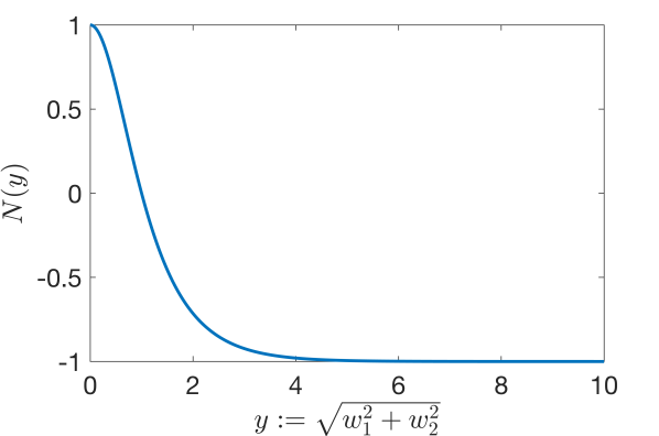
Figure 1: We present the picture of $N(w_{1},w_{2})$ with respect to the modulus $y=\sqrt{w_{1}^{2}+w_{2}^{2}}$.

From Table 1 to Table 4, we list $L^{2}$ errors in $w_{1},w_{2},b_{1},b_{2}$, and the corresponding numerical orders of accuracy subject to the variation of $q$ and $N$ at final time $T=1$ with the numerical fluxes given from (6.1) to (6.4). Note that the DG scheme (4.4)–(4.5) is developed for the characteristic variables $w_{1},w_{2}$; for completeness, we also include the errors in $b_{1}$ and $b_{2}$ by performing the linear transformation (2.1) to obtain the DG approximations $b_{1}^{h}$ and $b_{2}^{h}$. In particular, Table 2 and Table 3 present the results with conservative schemes: the central flux (6.2) and the mixed central flux (6.4), while Table 1 and Table 4 display the results with dissipating schemes: the upwind scheme (6.1) and the mixed upwind scheme (6.3).

For the energy dissipating scheme where the upwind flux or the mixed upwind scheme is implemented, from Table 1 or Table 4, we observe that the proposed scheme consistently gives the optimal $(q+1)$-th order of accuracy across the choices of the number of elements $N$ for the solutions $w_{1},w_{2},b_{1}$ and $b_{2}$.

For the energy conserving scheme where the central flux (6.2) is used, from Table 2, we note a super-convergence order $q+2$ when $q$ is even, while a sub-optimal convergence rate $q$ when $q$ is odd. Last, for the energy conserving scheme where the mixed central flux (6.4) is considered, from Table 3, we also observe an optimal convergence order $q+1$ though there are fluctuations, which is common for a conservative scheme since the initial error cannot be quickly damped.

		$w_{1}$		$w_{2}$		$b_{1}$		$b_{2}$
$q$	$N$	$L^{2}$ error	order	$L^{2}$ error	order	$L^{2}$ error	order	$L^{2}$ error	order
0	40	2.0618e-01	–	2.2555e-01	–	2.7714e-01	–	3.3160e-01	–
	80	1.2388e-01	0.7349	1.2250e-01	0.8807	1.5022e-01	0.8835	1.9529e-01	0.7638
	160	6.8560e-02	0.8536	6.3772e-02	0.9417	7.9408e-02	0.9197	1.0597e-01	0.8820
	320	3.6141e-02	0.9237	3.2518e-02	0.9717	4.1012e-02	0.9533	5.5183e-02	0.9413
	640	1.8563e-02	0.9612	1.6416e-02	0.9861	2.0866e-02	0.9749	2.8156e-02	0.9708
1	40	2.7426e-03	–	2.7172e-03	–	4.0346e-03	–	3.6786e-03	–
	80	6.5702e-04	2.0616	6.5526e-04	2.0520	9.5004e-04	2.0864	9.0527e-04	2.0228
	160	1.6186e-04	2.0212	1.6174e-04	2.0184	2.3167e-04	2.0359	2.2594e-04	2.0024
	320	4.0247e-05	2.0078	4.0240e-05	2.0070	5.7276e-05	2.0160	5.6548e-05	1.9984
	640	1.0040e-05	2.0031	1.0040e-05	2.0029	1.4244e-05	2.0075	1.4153e-05	1.9984
2	40	6.3391e-05	–	6.3341e-05	–	9.3036e-05	–	8.6053e-05	–
	80	7.8644e-06	3.0109	7.8629e-06	3.0100	1.1336e-05	3.0368	1.0901e-05	2.9807
	160	9.7931e-07	3.0055	9.7926e-07	3.0053	1.3984e-06	3.0191	1.3713e-06	2.9909
	320	1.2218e-07	3.0028	1.2218e-07	3.0027	1.7363e-07	3.0097	1.7194e-07	2.9956
	640	1.5257e-08	3.0014	1.5257e-08	3.0014	2.1630e-08	3.0049	2.1524e-08	2.9978
3	40	1.1951e-06	–	1.1960e-06	–	1.7589e-06	–	1.6197e-06	–
	80	7.4395e-08	4.0058	7.4413e-08	4.0065	1.0684e-07	4.0411	1.0358e-07	3.9669
	160	4.6378e-09	4.0037	4.6381e-09	4.0040	6.6103e-09	4.0146	6.5074e-09	3.9925
	320	2.8948e-10	4.0019	2.8948e-10	4.0020	4.1099e-10	4.0075	4.0777e-10	3.9962
	640	1.8080e-11	4.0009	1.8080e-11	4.0010	2.5619e-11	4.0038	2.5520e-11	3.9981

Table 1: $L^{2}$ errors and the corresponding convergence rates for $w_{1},w_{2},b_{1},b_{2}$ of problem (6.6) using $\mathcal{P}^{q}$ polynomials and the upwind flux (6.1). The interval is divided into $N$ uniform cells, and the terminal computational time is $T=1$.

		$w_{1}$		$w_{2}$		$b_{1}$		$b_{2}$
$q$	$N$	$L^{2}$ error	order	$L^{2}$ error	order	$L^{2}$ error	order	$L^{2}$ error	order
0	40	1.7427e-02	–	2.7306e-02	–	3.8033e-02	–	2.5536e-02	–
	80	4.3580e-03	1.9996	6.7582e-03	2.0145	9.5417e-03	1.9949	6.1877e-03	2.0450
	160	1.0896e-03	1.9999	1.6855e-03	2.0035	2.3878e-03	1.9985	1.5344e-03	2.0117
	320	2.7240e-04	2.0000	4.2112e-04	2.0009	5.9712e-04	1.9996	3.8281e-04	2.0030
	640	6.8101e-05	2.0000	1.0526e-04	2.0002	1.4929e-04	1.9999	9.5654e-05	2.0007
1	40	4.6923e-02	–	4.9988e-02	–	6.8179e-02	–	6.8940e-02	–
	80	2.3545e-02	0.9948	2.5185e-02	0.9890	3.2583e-02	1.0652	3.6272e-02	0.9265
	160	1.1781e-02	0.9989	1.2614e-02	0.9975	1.6092e-02	1.0178	1.8354e-02	0.9827
	320	5.8917e-03	0.9997	6.3097e-03	0.9994	8.0206e-03	1.0046	9.2044e-03	0.9957
	640	2.9460e-03	0.9999	3.1552e-03	0.9998	4.0071e-03	1.0011	4.6056e-03	0.9989
2	40	1.7123e-05	–	1.6677e-05	–	2.6737e-05	–	2.0682e-05	–
	80	6.0194e-07	4.8301	5.7921e-07	4.8476	8.7872e-07	4.9273	7.8961e-07	4.7111
	160	5.4792e-08	3.4576	5.3447e-08	3.4379	7.7657e-08	3.5002	7.5410e-08	3.3883
	320	2.3318e-09	4.5545	2.2482e-09	4.5713	3.2600e-09	4.5742	3.2180e-09	4.5505
	640	2.4289e-10	3.2631	2.3752e-10	3.2426	3.4132e-10	3.2556	3.3810e-10	3.2506
3	40	2.1038e-05	–	2.0260e-05	–	3.7819e-05	–	1.6610e-05	–
	80	2.7425e-06	2.9394	2.7826e-06	2.8641	4.1628e-06	3.1835	3.6332e-06	2.1927
	160	3.4322e-07	2.9983	3.5234e-07	2.9814	4.8917e-07	3.0891	4.9456e-07	2.8770
	320	4.2905e-08	2.9999	4.4170e-08	2.9958	6.0111e-08	3.0246	6.3010e-08	2.9725
	640	5.3632e-09	3.0000	5.5252e-09	2.9990	7.4811e-09	3.0063	7.9130e-09	2.9933

Table 2: $L^{2}$ errors and the corresponding convergence rates for $w_{1},w_{2},b_{1},b_{2}$ of problem (6.6) using $\mathcal{P}^{q}$ polynomials and the central flux (6.2). The interval is divided into $N$ uniform cells, and the terminal computational time is $T=1$.

		$w_{1}$		$w_{2}$		$b_{1}$		$b_{2}$
$q$	$N$	$L^{2}$ error	order	$L^{2}$ error	order	$L^{2}$ error	order	$L^{2}$ error	order
0	40	3.1939e-01	–	2.4017e-01	–	3.5673e-01	–	4.3832e-01	–
	80	1.5264e-01	1.0652	1.2336e-01	0.9612	1.6686e-01	1.0961	2.2179e-01	0.9828
	160	7.4617e-02	1.0325	6.2322e-02	0.9850	8.0635e-02	1.0492	1.1136e-01	0.9939
	320	3.6892e-02	1.0162	3.1302e-02	0.9935	3.9637e-02	1.0245	5.5772e-02	0.9976
	640	1.8343e-02	1.0081	1.5684e-02	0.9970	1.9652e-02	1.0122	2.7906e-02	0.9990
1	40	7.7379e-03	–	6.6755e-03	–	1.0531e-02	–	9.8986e-03	–
	80	9.3795e-04	3.0444	8.0919e-04	3.0443	1.2227e-03	3.1064	1.2546e-03	2.9800
	160	3.3209e-04	1.4979	3.1869e-04	1.3443	4.5389e-04	1.4297	4.6655e-04	1.4271
	320	1.1293e-04	1.5561	1.1180e-04	1.5112	1.5910e-04	1.5125	1.5873e-04	1.5555
	640	1.5939e-05	2.8248	1.5778e-05	2.8250	2.2371e-05	2.8302	2.2483e-05	2.8196
2	40	1.5944e-04	–	1.2786e-04	–	1.9650e-04	–	2.1196e-04	–
	80	1.0080e-05	3.9835	8.4746e-06	3.9152	1.2982e-05	3.9199	1.3352e-05	3.9886
	160	1.6531e-06	2.6081	1.5312e-06	2.4685	2.2696e-06	2.5160	2.2369e-06	2.5776
	320	2.9000e-07	2.5111	2.8078e-07	2.4471	4.0386e-07	2.4905	4.0345e-07	2.4710
	640	2.0669e-08	3.8105	2.0258e-08	3.7929	2.9057e-08	3.7969	2.8826e-08	3.8070
3	40	2.7237e-06	–	2.5996e-06	–	3.5133e-06	–	4.0012e-06	–
	80	1.8335e-07	3.8929	1.6457e-07	3.9815	2.5275e-07	3.7970	2.3983e-07	4.0603
	160	1.2695e-08	3.8522	1.2362e-08	3.7347	1.7513e-08	3.8512	1.7924e-08	3.7421
	320	5.4586e-10	4.5396	5.2741e-10	4.5508	7.6433e-10	4.5181	7.5370e-10	4.5718
	640	4.9108e-11	3.4745	4.8950e-11	3.4296	6.9477e-11	3.4596	6.9199e-11	3.4452

Table 3: $L^{2}$ errors and the corresponding convergence rates for $w_{1},w_{2},b_{1},b_{2}$ of problem (6.6) using $\mathcal{P}^{q}$ polynomials and the mixed central flux (6.4). The interval is divided into $N$ uniform cells, and the terminal computational time is $T=1$.

		$w_{1}$		$w_{2}$		$b_{1}$		$b_{2}$
$q$	$N$	$L^{2}$ error	order	$L^{2}$ error	order	$L^{2}$ error	order	$L^{2}$ error	order
0	40	2.8770e-01	–	2.4850e-01	–	3.7720e-01	–	3.8311e-01	–
	80	1.6003e-01	0.8463	1.3862e-01	0.8421	1.9287e-01	0.9677	2.2902e-01	0.7423
	160	8.5314e-02	0.9074	7.2910e-02	0.9270	9.7628e-02	0.9823	1.2513e-01	0.8720
	320	4.4175e-02	0.9496	3.7342e-02	0.9653	4.9162e-02	0.9897	6.5382e-02	0.9365
	640	2.2493e-02	0.9738	1.8891e-02	0.9831	2.4678e-02	0.9943	3.3416e-02	0.9684
1	40	1.8697e-03	–	1.9552e-03	–	2.6172e-03	–	2.7906e-03	–
	80	4.5582e-04	2.0363	4.6687e-04	2.0662	6.4279e-04	2.0256	6.6205e-04	2.0756
	160	1.1337e-04	2.0074	1.1480e-04	2.0239	1.6021e-04	2.0044	1.6247e-04	2.0268
	320	2.8326e-05	2.0009	2.8507e-05	2.0097	4.0051e-05	2.0001	4.0323e-05	2.0105
	640	7.0829e-06	1.9997	7.1058e-06	2.0043	1.0016e-05	1.9995	1.0050e-05	2.0045
2	40	9.6659e-05	–	7.9271e-05	–	1.3628e-04	–	1.1261e-04	–
	80	1.1624e-05	3.0558	1.0528e-05	2.9126	1.6425e-05	3.0526	1.4904e-05	2.9176
	160	1.4181e-06	3.0351	1.3498e-06	2.9634	2.0050e-06	3.0342	1.9094e-06	2.9645
	320	1.7491e-07	3.0193	1.7065e-07	2.9836	2.4734e-07	3.0190	2.4135e-07	2.9839
	640	2.1711e-08	3.0101	2.1446e-08	2.9923	3.0704e-08	3.0100	3.0330e-08	2.9923
3	40	8.3178e-07	–	9.0957e-07	–	1.1909e-06	–	1.2728e-06	–
	80	5.1621e-08	4.0102	5.4133e-08	4.0706	7.3144e-08	4.0252	7.6421e-08	4.0579
	160	3.2398e-09	3.9940	3.3172e-09	4.0284	4.5815e-09	3.9968	4.6916e-09	4.0258
	320	2.0341e-10	3.9935	2.0582e-10	4.0105	2.8766e-10	3.9934	2.9107e-10	4.0106
	640	1.2744e-11	3.9964	1.2819e-11	4.0050	1.8022e-11	3.9965	1.8130e-11	4.0049

Table 4: $L^{2}$ errors and the corresponding convergence rates for $w_{1},w_{2},b_{1},b_{2}$ of problem (6.6) using $\mathcal{P}^{q}$ polynomials and the mixed upwind flux (6.3). The interval is divided into $N$ uniform cells, and the terminal computational time is $T=1$.

In Figure 2, we report the errors in the solution $w_{1}$ (left) and $w_{2}$ (right) with respect to the spatial locations at the final time $T=1$ with the approximation order $q=3$, the number of elements $N=20,40,80$; from top to bottom are the results by using the upwind fluxes (6.1), the central fluxes (6.2), the mixed central fluxes (6.4), and the mixed upwind fluxes (6.3), respectively. We note that there is no severe error localization for both solutions $w_{1}$ and $w_{2}$ with four different numerical fluxes.

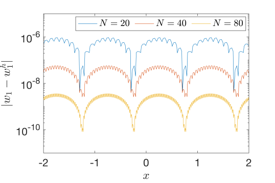
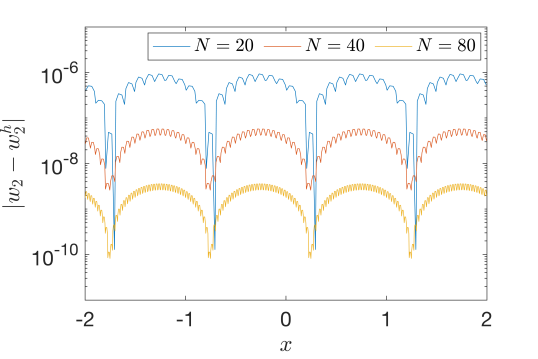
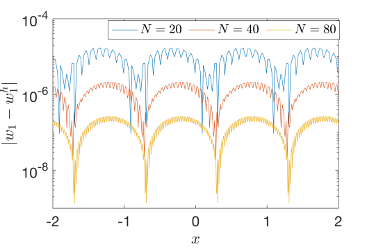
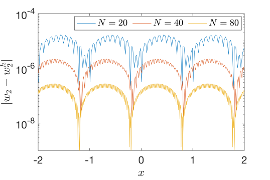
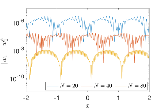
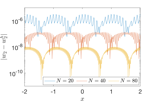
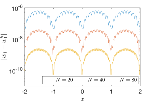
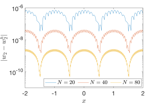
Figure 2: From the left to the right, we plot the errors $|w_{1}-w_{1}^{h}|$ and $|w_{2}-w_{2}^{h}|$ over the spatial location $x$ for the problem (6.5) using $\mathcal{P}^{3}$ polynomial on a uniform mesh of $N=20,40,80$; from the top to the bottom are the results by using the upwind fluxes (6.1), the central fluxes (6.2), the mixed central fluxes (6.4), and the mixed upwind fluxes (6.3), respectively.

6.1.2 Homogeneous Dirichlet boundary conditions

For the second example, we test a problem where the solution data decay to $0$ in the region near physical boundaries, i.e., near $x_{a}=-2$ and $x_{b}=2$. For simplicity, we still consider the same problem (6.6)–(6.7), but with the following manufactured solution

$$w_{1}=\sqrt{2}\Big{(}\cos(2\pi t)e^{-\frac{x^{2}}{0.01}}+2\cos(4\pi t)e^{-\frac{x^{2}}{0.025}}\Big{)},\quad w_{2}=\sqrt{2}\Big{(}\cos(2\pi t)e^{-\frac{x^{2}}{0.01}}-2\cos(4\pi t)e^{-\frac{x^{2}}{0.025}}\Big{)}.$$ (6.8)

With the same spatial discretization as conducted in Section 6.1.1, we also present the $L^{2}$ errors in solutions $w_{1},w_{2},b_{1},b_{2}$ from Table 5 to Table 8 with four different numerical fluxes defined from (6.1) to (6.4). We observe the same results with the first example (6.5): optimal convergence order $q+1$ for the dissipating schemes, the upwind flux (6.1) in Table 5 and the mixed upwind scheme (6.3) in Table 4; super-convergence rate $q+2$ for the central flux (6.2) when $q$ is even, while a sub-optimal convergence rate $q$ when $q$ is odd as presented in Table 6; when the mixed central flux (6.4) is implemented displayed in Table 7, an optimal convergence order $q+1$ is obtained, but there are some fluctuations for this energy conservative scheme.

		$w_{1}$		$w_{2}$		$b_{1}$		$b_{2}$
$q$	$N$	$L^{2}$ error	order	$L^{2}$ error	order	$L^{2}$ error	order	$L^{2}$ error	order
0	40	3.4682e-01	–	1.6750e-01	–	2.7693e-01	–	4.6903e-01	–
	80	2.2832e-01	0.6032	1.8108e-01	-0.1125	2.0982e-01	0.4003	3.5470e-01	0.4031
	160	1.4636e-01	0.6415	1.5203e-01	0.2523	1.7072e-01	0.2975	2.4479e-01	0.5351
	320	9.2281e-02	0.6654	1.0447e-01	0.5413	1.2168e-01	0.4886	1.5509e-01	0.6585
	640	5.5131e-02	0.7432	6.2669e-02	0.7372	7.5532e-02	0.6879	9.0712e-02	0.7737
1	40	6.5776e-02	–	4.1806e-02	–	7.8510e-02	–	7.7361e-02	–
	80	1.6044e-02	2.0355	7.7474e-03	2.4319	1.8100e-02	2.1169	1.7530e-02	2.1418
	160	3.7870e-03	2.0829	1.4300e-03	2.4377	4.1830e-03	2.1134	3.9084e-03	2.1651
	320	9.2584e-04	2.0322	3.1078e-04	2.2021	1.0144e-03	2.0439	9.3726e-04	2.0601
	640	2.3002e-04	2.0090	7.4325e-05	2.0640	2.5150e-04	2.0120	2.3155e-04	2.0172
2	40	9.0106e-03	–	4.0634e-03	–	7.4050e-03	–	1.1856e-02	–
	80	1.0237e-03	3.1378	4.1478e-04	3.2923	9.3769e-04	2.9813	1.2493e-03	3.2465
	160	1.2889e-04	2.9896	5.2273e-05	2.9882	1.1600e-04	3.0150	1.5885e-04	2.9754
	320	1.6149e-05	2.9966	6.5466e-06	2.9972	1.4479e-05	3.0021	1.9941e-05	2.9939
	640	2.0200e-06	2.9990	8.1840e-07	2.9999	1.8099e-06	2.9999	2.4949e-06	2.9987
3	40	6.9888e-04	–	2.9768e-04	–	9.5778e-04	–	4.8660e-04	–
	80	6.9326e-05	3.3336	3.7505e-05	2.9886	5.0811e-05	4.2365	9.9215e-05	2.2941
	160	4.3839e-06	3.9831	2.3764e-06	3.9802	3.1020e-06	4.0339	6.3332e-06	3.9696
	320	2.7492e-07	3.9951	1.4898e-07	3.9955	1.9294e-07	4.0070	3.9790e-07	3.9924
	640	1.7199e-08	3.9986	9.3152e-09	3.9994	1.2048e-08	4.0012	2.4899e-08	3.9982

Table 5: $L^{2}$ errors and the corresponding convergence rates for $w_{1},w_{2},b_{1},b_{2}$ of problem (6.8) using $\mathcal{P}^{q}$ polynomials and the upwind flux (6.1). The interval is divided into $N$ uniform cells, and the terminal computational time is $T=1$.

		$w_{1}$		$w_{2}$		$b_{1}$		$b_{2}$
$q$	$N$	$L^{2}$ error	order	$L^{2}$ error	order	$L^{2}$ error	order	$L^{2}$ error	order
0	40	4.3279e-01	–	8.6203e-01	–	8.5573e-01	–	1.0623e+00	–
	80	1.5428e-01	1.4882	1.3085e-01	2.7199	2.1157e-01	2.0160	1.9256e-01	2.4638
	160	3.4830e-02	2.1471	2.9357e-02	2.1561	4.7421e-02	2.1576	4.3602e-02	2.1428
	320	8.4962e-03	2.0355	7.1608e-03	2.0355	1.1543e-02	2.0385	1.0662e-02	2.0319
	640	2.1117e-03	2.0084	1.7798e-03	2.0084	2.8679e-03	2.0090	2.6513e-03	2.0077
1	40	1.5483e-01	–	1.0178e-01	–	1.6979e-01	–	1.9959e-01	–
	80	6.7997e-02	1.1872	4.4655e-02	1.1886	7.1201e-02	1.2538	9.0364e-02	1.1432
	160	3.2712e-02	1.0557	2.1182e-02	1.0759	3.3579e-02	1.0843	4.3703e-02	1.0480
	320	1.6196e-02	1.0142	1.0453e-02	1.0189	1.6534e-02	1.0221	2.1675e-02	1.0117
	640	8.0776e-03	1.0036	5.2092e-03	1.0048	8.2345e-03	1.0057	1.0815e-02	1.0030
2	40	5.4484e-02	–	5.5823e-02	–	7.8592e-02	–	7.7412e-02	–
	80	7.2114e-04	6.2394	4.2114e-04	7.0504	9.7526e-04	6.3325	6.6609e-04	6.8607
	160	4.2372e-05	4.0891	2.4013e-05	4.1324	5.7785e-05	4.0770	3.7483e-05	4.1514
	320	2.3909e-06	4.1475	1.4440e-06	4.0556	3.2248e-06	4.1634	2.2813e-06	4.0383
	640	1.4802e-07	4.0137	8.4411e-08	4.0965	1.9563e-07	4.0430	1.4071e-07	4.0191
3	40	9.6599e-04	–	3.8383e-04	–	9.9817e-04	–	1.0791e-03	–
	80	1.4126e-04	2.7736	5.7700e-05	2.7338	1.6239e-04	2.6199	1.4212e-04	2.9247
	160	1.6458e-05	3.1015	7.1899e-06	3.0045	2.0128e-05	3.0121	1.5490e-05	3.1977
	320	1.9666e-06	3.0650	7.9819e-07	3.1712	2.3930e-06	3.0723	1.8120e-06	3.0957
	640	2.4608e-07	2.9985	9.9923e-08	2.9978	3.0224e-07	2.9850	2.2301e-07	3.0224

Table 6: $L^{2}$ errors and the corresponding convergence rates for $w_{1},w_{2},b_{1},b_{2}$ of problem (6.8) using $\mathcal{P}^{q}$ polynomials and the central flux (6.2). The interval is divided into $N$ uniform cells, and the terminal computational time is $T=1$.

		$w_{1}$		$w_{2}$		$b_{1}$		$b_{2}$
$q$	$N$	$L^{2}$ error	order	$L^{2}$ error	order	$L^{2}$ error	order	$L^{2}$ error	order
0	40	1.1420e+00	–	1.0684e+00	–	1.6597e+00	–	1.4617e+00	–
	80	5.6375e-01	1.0184	5.7341e-01	0.8978	8.5070e-01	0.9642	7.5467e-01	0.9538
	160	2.7904e-01	1.0146	2.9644e-01	0.9518	4.3075e-01	0.9818	3.8201e-01	0.9822
	320	1.3942e-01	1.0011	1.5073e-01	0.9757	2.1747e-01	0.9860	1.9241e-01	0.9894
	640	6.9812e-02	0.9978	7.5997e-02	0.9880	1.0940e-01	0.9912	9.6589e-02	0.9942
1	40	6.0056e-02	–	8.9200e-02	–	1.0663e-01	–	1.0843e-01	–
	80	1.2054e-02	2.3168	2.0543e-02	2.1184	2.6396e-02	2.0143	2.0926e-02	2.3733
	160	3.1799e-03	1.9224	2.5745e-03	2.9963	3.9940e-03	2.7244	4.1866e-03	2.3214
	320	7.9069e-04	2.0078	1.4214e-03	0.8570	8.3806e-04	2.2527	2.1421e-03	0.9668
	640	2.2029e-04	1.8437	1.5592e-04	3.1884	3.3500e-04	1.3229	1.8288e-04	3.5501
2	40	5.9545e-03	–	1.4531e-02	–	1.8142e-02	–	1.2809e-02	–
	80	8.5996e-04	2.7916	1.3745e-03	3.4022	1.6622e-03	3.4482	1.5794e-03	3.0197
	160	9.9033e-05	3.1183	1.8951e-04	2.8585	2.1876e-04	2.9257	2.0878e-04	2.9193
	320	1.1776e-05	3.0721	2.3327e-05	3.0222	2.3848e-05	3.1974	2.8230e-05	2.8867
	640	1.3547e-06	3.1197	7.7926e-07	4.9037	1.5916e-06	3.9053	1.5336e-06	4.2022
3	40	5.5938e-04	–	9.2006e-04	–	1.2434e-03	–	8.7905e-04	–
	80	6.0453e-05	3.2100	9.4019e-05	3.2907	1.1651e-04	3.4158	1.0684e-04	3.0405
	160	3.9276e-06	3.9441	4.9625e-06	4.2438	6.0736e-06	4.2617	6.5739e-06	4.0225
	320	3.4942e-07	3.4906	3.6036e-07	3.7836	6.6399e-07	3.1933	2.5104e-07	4.7108
	640	1.6524e-08	4.4023	2.9671e-08	3.6023	4.2447e-08	3.9674	2.2473e-08	3.4817

Table 7: $L^{2}$ errors and the corresponding convergence rates for $w_{1},w_{2},b_{1},b_{2}$ of problem (6.8) using $\mathcal{P}^{q}$ polynomials and the mixed central flux (6.4). The interval is divided into $N$ uniform cells, and the terminal computational time is $T=1$.

		$w_{1}$		$w_{2}$		$b_{1}$		$b_{2}$
$q$	$N$	$L^{2}$ error	order	$L^{2}$ error	order	$L^{2}$ error	order	$L^{2}$ error	order
0	40	4.7347e-01	–	2.4353e-01	–	6.0749e-01	–	4.4487e-01	–
	80	3.5425e-01	0.4185	1.8822e-01	0.3716	4.3451e-01	0.4835	3.6475e-01	0.2865
	160	2.5777e-01	0.4587	1.1979e-01	0.6519	2.9064e-01	0.5801	2.7771e-01	0.3933
	320	1.7288e-01	0.5764	6.9034e-02	0.7951	1.8549e-01	0.6479	1.8681e-01	0.5720
	640	1.0479e-01	0.7223	3.8201e-02	0.8537	1.1043e-01	0.7482	1.1262e-01	0.7301
1	40	6.5922e-02	–	3.3550e-02	–	5.8441e-02	–	8.6760e-02	–
	80	1.0901e-02	2.5964	8.6228e-03	1.9601	8.8293e-03	2.7266	1.7561e-02	2.3046
	160	2.2018e-03	2.3076	1.9331e-03	2.1572	1.5023e-03	2.5552	3.8618e-03	2.1850
	320	5.1385e-04	2.0993	4.6666e-04	2.0505	3.1504e-04	2.2535	9.2972e-04	2.0544
	640	1.2616e-04	2.0261	1.1560e-04	2.0133	7.4564e-05	2.0790	2.3021e-04	2.0138
2	40	5.9664e-03	–	6.5599e-03	–	5.5459e-03	–	1.1247e-02	–
	80	9.1259e-04	2.7088	9.5240e-04	2.7840	8.4156e-04	2.7203	1.6648e-03	2.7562
	160	1.1692e-04	2.9645	1.4525e-04	2.7131	1.0732e-04	2.9712	2.4087e-04	2.7890
	320	1.4532e-05	3.0082	1.9448e-05	2.9008	1.3222e-05	3.0209	3.1686e-05	2.9263
	640	1.8113e-06	3.0041	2.4783e-06	2.9722	1.6409e-06	3.0104	4.0191e-06	2.9789
3	40	6.2444e-04	–	4.5116e-04	–	5.8689e-04	–	9.1789e-04	–
	80	2.9422e-05	4.4076	6.5006e-05	2.7950	5.3307e-05	3.4607	8.5681e-05	3.4213
	160	1.6370e-06	4.1678	3.4026e-06	4.2559	2.6600e-06	4.3248	4.6302e-06	4.2098
	320	9.7929e-08	4.0631	2.0255e-07	4.0703	1.5352e-07	4.1149	2.7869e-07	4.0543
	640	6.0479e-09	4.0172	1.2504e-08	4.0178	9.3843e-09	4.0321	1.7257e-08	4.0134

Table 8: $L^{2}$ errors and the corresponding convergence rates for $w_{1},w_{2},b_{1},b_{2}$ of problem (6.8) using $\mathcal{P}^{q}$ polynomials and the mixed upwind flux (6.3). The interval is divided into $N$ uniform cells, and the terminal computational time is $T=1$.

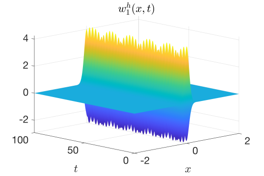
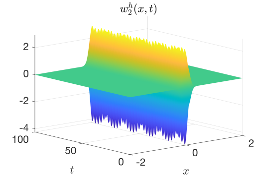
Figure 3: Space-time plots of the solutions of problem (6.8) with the degree of approximation space $q=3$. The upwind fluxes (6.1) is used in the simulation.

We also present the solutions of the problem (6.8) in Figure 4 and Figure 3. In the simulation, the approximation degrees for $w_{1}^{h}$ and $w_{2}^{h}$ are $q=3$, and the upwind flux (6.1) is used. Figure 4 displays both the numerical solutions $w_{1}^{h},w_{2}^{h}$ and the exact solutions $w_{1},w_{2}$ at $t=0,30,75,100$; while Figure 3 presents the space-time plot of the solutions (6.8) from $t=0$ to $t=100$. We find that the numerical results match well with the analytic solution for a very long time.

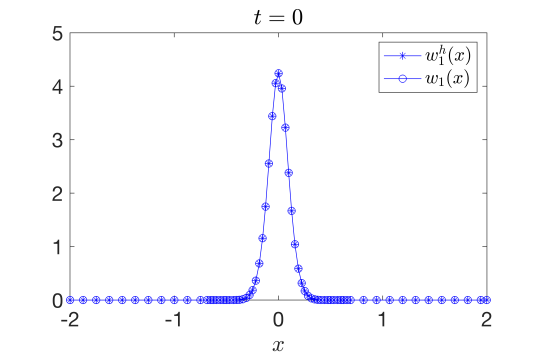
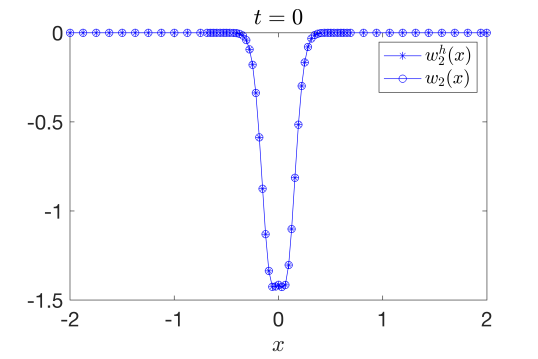
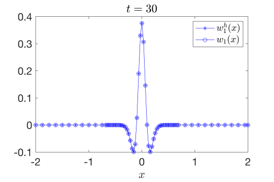
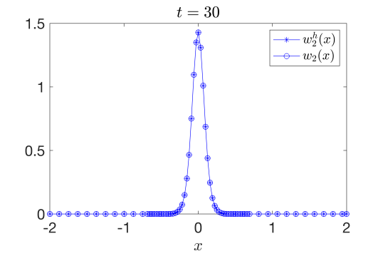
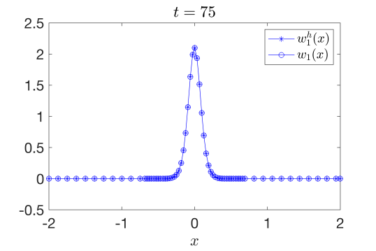
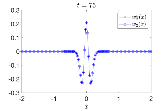
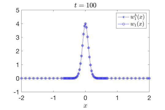
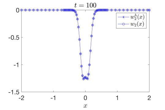
Figure 4: Plots of both the numerical solutions $w_{1}^{h},w_{2}^{h}$, and the exact solutions $w_{1},w_{2}$ of problem (6.8) with the degree of approximation space $q=3$. The upwind fluxes (6.1) is used in the simulation. The numerical and exact solutions at $t=0,30,75,100$ are plotted from top to bottom. On the left, we present the results for $w_{1}$, while on the right, we display the results for $w_{2}$.

6.2 Kink solitons

Here, we consider the traveling wave-like solutions of the system (2.2). Let

$$w_{1}(x,t)=w_{1}(x-ct),\quad w_{2}(x,t)=w_{2}(x-ct),$$

then system (2.2) can be rewritten to the following ODE system,

$$(c+1)\frac{dw_{1}}{dz} =N(w_{1},w_{2})w_{2},$$ (6.9)

$$(1-c)\frac{dw_{2}}{dz} =N(w_{1},w_{2})w_{1},$$

where $z:=x-ct$, and the nonlinear interaction, $N(w_{1},w_{2})$, is specified the same as the one in example one, see (6.7). When $|c|\neq 1$, we have

$$(w_{1},w_{2})=(0,0)\ \ \mbox{and}\ \ (w_{1},w_{2})=(\cos\theta,\sin\theta),\ \theta\in(0,2\pi]$$

are fixed points of the ODE system (6.9). As shown in [36], we have

$$\frac{dQ\big{(}w_{1}(z),w_{2}(z)\big{)}}{dz}=0,$$

where

$$Q\big{(}w_{1}(z),w_{2}(z)\big{)}=c\left(\frac{(w_{1}+w_{2})^{2}}{2}+\frac{(w_{1}-w_{2})^{2}}{2}\right)+w_{1}^{2}-w_{2}^{2}.$$ (6.10)

This indicates that for a given constant $Q$, (6.10) can only be unbounded, periodic, a fixed point, or approaches fixed points of (6.9). We have the so-called kink solitons when $|c|<1$ and the solutions with nontrivial asymptotic values at either $+\infty$ or $-\infty$. We refer to [36] for more extensive discussions.

In this section, we numerically study the dynamics of these kink solitons of the system (2.2) by the proposed DG scheme in Section 4 with the upwind fluxes (6.1).

To this end, we consider problem (2.2) in a computational domain defined from $x_{a}=-40$ to $x_{b}=200$, the wave speed is chosen to be $c=0.4<1$, and the degree of the approximation space is set as $q=(0,1,2,3)$. In addition, we discretize the computational domain by a uniform mesh with DG element vertices $x_{i}=x_{a}+ih,i=0,1,\cdots,600$, namely, $h=0.4$. The problem is evolved with the classical $4$-stage Runge Kutta time integrator until the final time $T=100$ with time step size $\Delta_{t}=4\times 10^{-5}$.

An accurate initial data profile, given by a kink solution, is generated as follows. We perturb the trivial fixed point, $(w_{1},w_{2})=(0,0)$, of the ODE system (6.9) to make

$$w_{1}(z=0)=-7\sqrt{2}\times 10^{-51},\quad w_{2}(z=0)=-3\sqrt{2}\times 10^{-51}$$

be the initial data, then implement MATLAB inline function $ode45$ to solve (6.9). In particular, when calling $ode45$, we set the termination time to be coincidental with spatial Gauss nodes, then followed by setting $t=0$ in $z=x-ct$ of the resulting ODE system solution, we obtain the initial profile for the original PDE system (2.2), see Figure 5. In addition, we impose Dirichlet boundary conditions when numerically solving the problem (2.2).

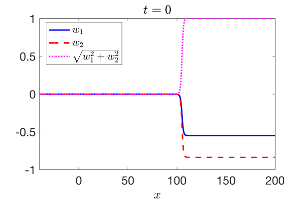
Figure 5: Initial profiles, $(w_{1}(x,0),w_{2}(x,0))$, of the kink solutions of the system (2.2).

Figure 6 (resp. Figure 7) presents the space-time plots of $w_{1}^{h}$ (resp. $w_{2}^{h}$), while Figure 8 displays the comparison between numerical solutions with different approximation degree $q$ at final time $t=100$: on the left is the plot for $w_{1}^{h}$ and on the right is for $w_{2}^{h}$. In addition, Figure 6 and Figure 7 have the same layout: from left to right are the kink solitons with the degree of approximation space $q=0,q=1,q=2$ and $q=3$, respectively. From these figures, we see that when the degree of the approximation space is very small, say $q=0$, non-physical oscillations are generated near the fast transition region of the kink solitons and then move to the left with the oscillations being weaker and weaker, but make the kink solitons a small phase shift to the right. When the degree of the approximation is relatively large, for this example $q\geq 1$, we see that the kink soliton, $w_{1}^{h}$, decreases monotonically from $0$ to $\sim-0.5477$ in Figure 6, while decreases monotonically from $0$ to $\sim-0.8366$ for the kink soliton, $w_{2}^{h}$, in Figure 7. And they move from the left to the right with their original shape.

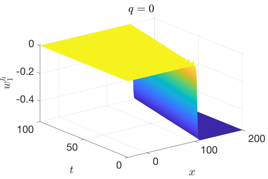
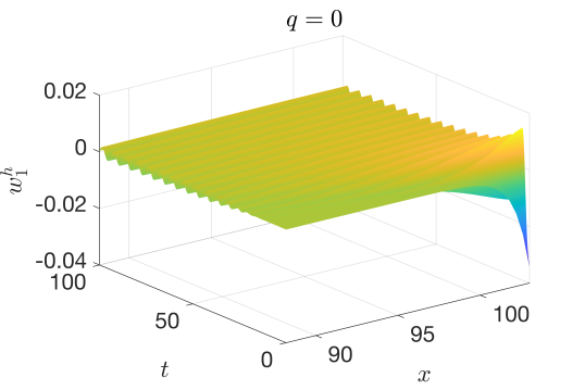
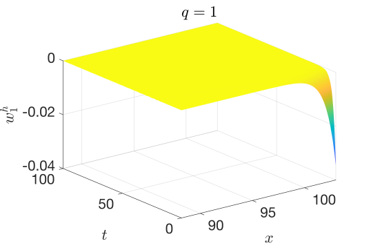
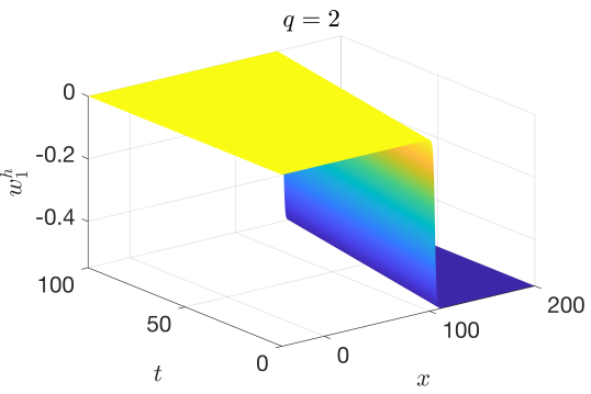
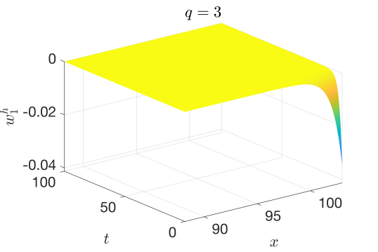
Figure 6: Space-time plots of $w_{1}^{h}(x,t)$. On the left panel, from the top to the bottom are the plots for the kink soliton with $q=0$, $q=1$, $q=2$, and $q=3$ respectively; On the right panel are the zoom in plots of the transition region, $x\in(88,103)$, of the kink soliton.

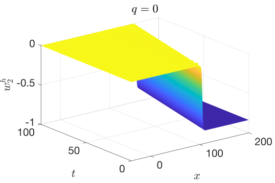
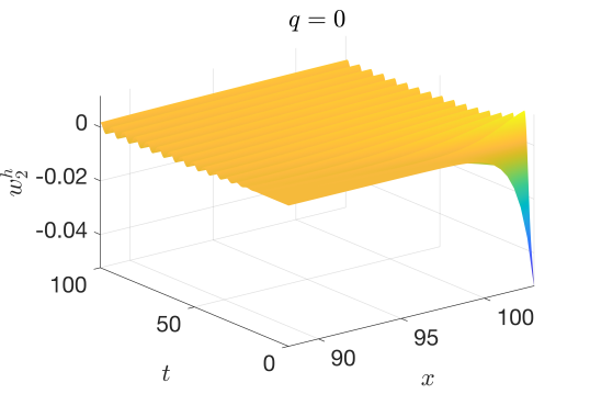
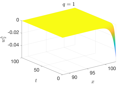
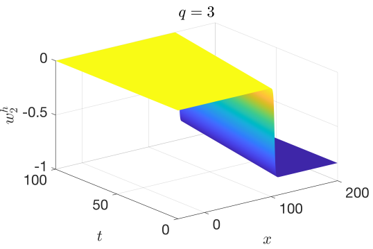
Figure 7: Space-time plots of $w_{2}^{h}(x,t)$. On the left panel, from top to bottom, are the plots for the kink soliton with $q=0$, $q=1$, $q=2$, and $q=3$, respectively; On the right panel are the zoom-in plots of the transition region, $x\in(88,103)$, of the kink soliton.

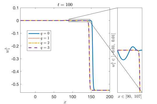
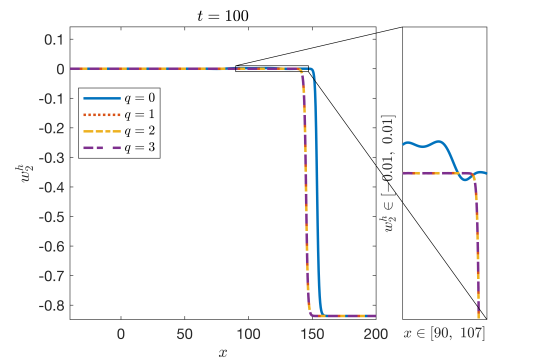
Figure 8: Comparison between the kink solitons with different degrees of approximation space $q$ at the final time $t=100$. On the left presents the results for $w_{1}^{h}$, and the right shows the results for $w_{2}^{h}$.

Last, the numerical discrete energy $E^{h}(t)$, defined in (4.7), trajectories of the proposed DG scheme for the problem (2.2) until the final time $t=100$ with the initial profile shown in Figure 5 are presented in Figure 9 with different degrees, $q$, of the approximation space. Particularly, to measure the performance of the schemes with different approximation degrees $q$, we compute the numerical discrete energy $E^{h}(t)$ in a moving box that has the same speed $c=0.4$ with the kink solitons. Initially, the box is located from $x=60$ to $x=140$. Overall, we note that the discrete energy is dissipating as predicted since we use an energy dissipating scheme, the upwind fluxes (6.1), for the simulations here. In addition, we observe that when $q=0$, the energy dissipates a lot since there are non-physical oscillations generated as shown in Figure 6 and Figure 7. When $q=1,2,3$, though the energy is dissipating as predicted, the total dissipation is small, and the changes happen only around the third digit for $q=1$, around $5$ digits for $q=2$, and around $8$ digits for $q=3$ until $T=100$. One quick takeaway from this is that high-order schemes have better performance, and lower dispersion and dissipation errors, than their lower-order counterparts.

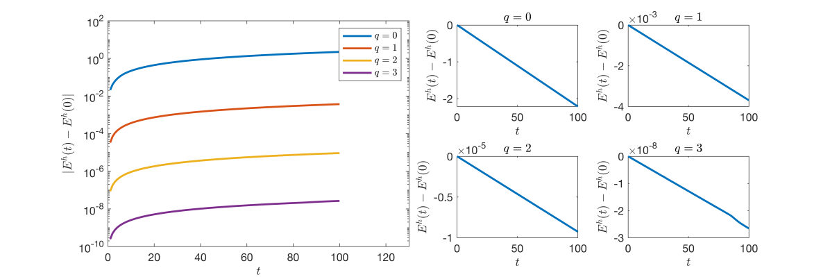
Figure 9: we present the energy difference, $|E^{h}(t)-E^{h}(0)|$ on the left and $E^{h}(t)-E^{h}(0)$ on the right, of kink solitons with different degrees $q$ of approximation space in a moving box until the final time $T=100$. The box is initially put at the region of $x\in[60,140]$ and then moves to the right with the same speed as the kink solitons.

7 Conclusion

In this work, a DG method is developed and analyzed for a first-order semi-linear hyperbolic system modeling a dimer lattice. The stability of the semi-discrete DG formulation is proved and demonstrated for general mesh-independent numerical fluxes; moreover, we also show optimal $L^{2}$-error estimates for the upwind fluxes with periodic boundary conditions. Our numerical experiments verify the theoretical findings. In addition, when using mixed fluxes, we also numerically observed the optimal convergence in the $L^{2}$ norm; for the central fluxes, we observe a sub-optimal convergence for polynomials of odd degrees, but a super-convergence for polynomials of even degrees. This phenomenon is common in literature when central fluxes are used; indeed, Bassi et al. [2] reported an optimal convergence order $q+1$ for even values of $q$ and a suboptimal convergence order $q$ for the odd value of $q$ for a purely elliptic problem with uniform grids. Cockburn and Shu [17] also presented the same results for a purely parabolic problem; see their Table 5. In addition, Delfour et al. [19] reported this phenomenon in the framework of ODEs, see their Table A. Applications to kink solitons have demonstrated the effectiveness of high-order numerical schemes. Our main target for future work will be extensions to problems in multi-dimensional space. This will enable applications to a wider variety of problems of physical interest. We will also devote our effort to the development of an energy-conserving fully-discrete DG scheme for the proposed problem, which will be more favorable when simulating waves with long time integration since they can maintain the phase and shape of the waves accurately.

Funding

This work is partially supported by US National Science Foundation grant DMS-2012562 (QD), DMS-1937254 (QD and MW), DMS-1620418 (MW and HL), DMS-1908657 (MW and HL), and Simons Foundation Math + X Investigator Award #376319 (MW).

References

- [1] Daniel Appelö, Thomas Hagstrom, Qi Wang, and Lu Zhang. An energy-based discontinuous Galerkin method for semilinear wave equations. Journal of Computational Physics, 418:109608, 2020.
- [2] Francesco Bassi, Stefano Rebay, Gianluca Mariotti, Savini Pedinotti, and Marco Savini. A high-order accurate discontinuous finite element method for inviscid and viscous turbomachinery flows. In Proceedings of the 2nd European Conference on Turbomachinery Fluid Dynamics and Thermodynamics, pages 99–109. Antwerpen, Belgium, 1997.
- [3] Richard M Beam and Robert F Warming. An implicit finite-difference algorithm for hyperbolic systems in conservation-law form. Journal of computational physics, 22(1):87–110, 1976.
- [4] Rajesh Chaunsali and Georgios Theocharis. Self-induced topological transition in phononic crystals by nonlinearity management. Physical Review B, 100(1):014302, 2019.
- [5] Rajesh Chaunsali and Georgios Theocharis. Self-induced topological transition in phononic crystals by nonlinearity management. Physical Review B, 100:014302, 2019.
- [6] Rajesh Chaunsali, Haitao Xu, Jinkyu Yang, Panayotis G. Kevrekidis, and Georgios Theocharis. Stability of topological edge states under strong nonlinear effects. Physical Review B, 103:024106, 2021.
- [7] Eric T Chung and Björn Engquist. Optimal discontinuous Galerkin methods for wave propagation. SIAM Journal on Numerical Analysis, 44(5):2131–2158, 2006.
- [8] Eric T Chung and Björn Engquist. Optimal discontinuous Galerkin methods for the acoustic wave equation in higher dimensions. SIAM Journal on Numerical Analysis, 47(5):3820–3848, 2009.
- [9] Philippe G Ciarlet. The finite element method for elliptic problems. SIAM, 2002.
- [10] Bernardo Cockburn. Discontinuous Galerkin methods for computational fluid dynamics. Encyclopedia of Computational Mechanics Second Edition, pages 1–63, 2018.
- [11] Bernardo Cockburn, Suchung Hou, and Chi-Wang Shu. The Runge-Kutta local projection discontinuous Galerkin finite element method for conservation laws IV: The multidimensional case. Mathematics of Computation, 54(190):545–581, 1990.
- [12] Bernardo Cockburn, George E Karniadakis, and Chi-Wang Shu. The development of discontinuous Galerkin methods. In Discontinuous Galerkin Methods, pages 3–50. Springer, 2000.
- [13] Bernardo Cockburn, San-Yih Lin, and Chi-Wang Shu. TVB Runge-Kutta local projection discontinuous Galerkin finite element method for conservation laws III: one-dimensional systems. Journal of computational Physics, 84(1):90–113, 1989.
- [14] Bernardo Cockburn, Mitchell Luskin, Chi-Wang Shu, and Endre Süli. Enhanced accuracy by post-processing for finite element methods for hyperbolic equations. Mathematics of Computation, 72(242):577–606, 2003.
- [15] Bernardo Cockburn and Chi-Wang Shu. TVB Runge-Kutta local projection discontinuous Galerkin finite element method for conservation laws II: General framework. Mathematics of computation, 52(186):411–435, 1989.
- [16] Bernardo Cockburn and Chi-Wang Shu. The Runge-Kutta local projection -discontinuous-Galerkin finite element method for scalar conservation laws. ESAIM: Mathematical Modelling and Numerical Analysis, 25(3), 1991.
- [17] Bernardo Cockburn and Chi-Wang Shu. The local discontinuous Galerkin method for time-dependent convection-diffusion systems. SIAM journal on numerical analysis, 35(6):2440–2463, 1998.
- [18] Bernardo Cockburn and Chi-Wang Shu. The Runge–Kutta discontinuous Galerkin method for conservation laws V: multidimensional systems. Journal of Computational Physics, 141(2):199–224, 1998.
- [19] Michel Delfour, William Hager, and François Trochu. Discontinuous Galerkin methods for ordinary differential equations. mathematics of computation, 36(154):455–473, 1981.
- [20] Michael Dumbser, Martin Käser, Vladimir A Titarev, and Eleuterio F Toro. Quadrature-free non-oscillatory finite volume schemes on unstructured meshes for nonlinear hyperbolic systems. Journal of Computational Physics, 226(1):204–243, 2007.
- [21] Bjorn Engquist and Thomas Y Hou. Particle method approximation of oscillatory solutions to hyperbolic differential equations. SIAM journal on numerical analysis, 26(2):289–319, 1989.
- [22] David Gottlieb and Jan S Hesthaven. Spectral methods for hyperbolic problems. Journal of Computational and Applied Mathematics, 128(1-2):83–131, 2001.
- [23] Yakir Hadad, Vincenzo Vitelli, and Andrea Alu. Solitons and propagating domain walls in topological resonator arrays. ACS Photonics, 4(8):1974–1979, 2017.
- [24] Yakir Hadad, Vincenzo Vitelli, and Andrea Alu. Solitons and propagating domain walls in topological resonator arrays. ACS Photonics, 4:1974–1979, 2017.
- [25] Frederick Haldane, Duncan Michael, and Srinivas Raghu. Possible realization of directional optical waveguides in photonic crystals with broken time-reversal symmetry. Physical review letters, 100(1):013904, 2008.
- [26] M. Zahid Hasan and Charles L. Kane. Colloquium: topological insulators. Reviews of Modern Physics, 82:3045, 2010.
- [27] Alan J Heeger, Steven Kivelson, John Robert Schrieffer, and Wu-Pei Su. Solitons in conducting polymers. Reviews of Modern Physics, 60(3):781, 1988.
- [28] Jan S Hesthaven and Tim Warburton. Nodal discontinuous Galerkin methods: algorithms, analysis, and applications. Springer Science & Business Media, 2007.
- [29] Sebastian D Huber. Topological mechanics. Nature Physics, 12(7):621–623, 2016.
- [30] Lucien Jezequel and Pierre Delplace. Nonlinear edge modes from topological one-dimensional lattices. Physical Review B, 105:035410, 2022.
- [31] Claes Johnson, Uno Nävert, and Juhani Pitkäranta. Finite element methods for linear hyperbolic problems. Computer methods in applied mechanics and engineering, 45(1-3):285–312, 1984.
- [32] Klaus Von Klitzing, Gerhard Dorda, and Michael Pepper. New method for high-accuracy determination of the fine-structure constant based on quantized hall resistance. Physical Review Letters, 45:494–497, 1980.
- [33] Pierre Lesaint. Finite element methods for symmetric hyperbolic equations. Numerische Mathematik, 21(3):244–255, 1973.
- [34] Pierre Lesaint and Pierre-Arnaud Raviart. On a finite element method for solving the neutron transport equation. Publications mathématiques et informatique de Rennes, (S4):1–40, 1974.
- [35] Randall J LeVeque et al. Finite volume methods for hyperbolic problems, volume 31. Cambridge university press, 2002.
- [36] Huaiyu Li, Andrew Hofstrand, and Michael I. Weinstein. Coherent structures on a dimer lattice. Preprint.
- [37] Ling Lu, John D Joannopoulos, and Marin Soljačić. Topological photonics. Nature photonics, 8(11):821–829, 2014.
- [38] S. Hossein Mousavi, Alexander B. Khanikaev, and Zheng Wang. Topologically protected elastic waves in phononic metamaterials. Nature Communications, 6, 2015.
- [39] Ngoc Cuong Nguyen, Jaume Peraire, and Bernardo Cockburn. High-order implicit hybridizable discontinuous Galerkin methods for acoustics and elastodynamics. Journal of Computational Physics, 230(10):3695–3718, 2011.
- [40] Tomoki Ozawa, Hannah M. Price, Alberto Amo, Nathan Goldman, Mohammad Hafezi, Ling Lu, Mikael C. Rechtsman, David Schuster, Jonathan Simon, Oded Zilberberg, and Iacopo Carusotto. Topological photonics. Reviews of Modern Physics, 91, 2019.
- [41] Todd E Peterson. A note on the convergence of the discontinuous Galerkin method for a scalar hyperbolic equation. SIAM Journal on Numerical Analysis, 28(1):133–140, 1991.
- [42] Pierre-Arnaud Raviart. An analysis of particle methods. In Numerical methods in fluid dynamics, pages 243–324. Springer, 1985.
- [43] William H Reed and Thomas R Hill. Triangular mesh methods for the neutron transport equation. Technical report, Los Alamos Scientific Lab., N. Mex.(USA), 1973.
- [44] Andrés M Rueda-Ramírez, Florian J Hindenlang, Jesse Chan, and Gregor J Gassner. Entropy-stable Gauss collocation methods for ideal magneto-hydrodynamics. arXiv preprint arXiv:2203.06062, 2022.
- [45] Chi-Wang Shu. Discontinuous Galerkin method for time-dependent problems: survey and recent developments. Recent developments in discontinuous Galerkin finite element methods for partial differential equations, pages 25–62, 2014.
- [46] Daria Smirnova, Daniel Leykam, Yidong Chong, and Yuri Kivshar. Nonlinear topological photonics. Applied Physics Reviews, 7:021306, 2020.
- [47] Daria Smirnova, Daniel Leykam, Yidong Chong, and Yuri Kivshar. Nonlinear topological photonics. Applied Physics Reviews, 7(2):021306, 2020.
- [48] Gary A Sod. A survey of several finite difference methods for systems of nonlinear hyperbolic conservation laws. Journal of computational physics, 27(1):1–31, 1978.
- [49] Wu-Pei Su, John Robert Schrieffer, and Alan J Heeger. Solitons in polyacetylene. Physical review letters, 42(25):1698, 1979.
- [50] Eitan Tadmor. Convergence of spectral methods for nonlinear conservation laws. SIAM Journal on Numerical Analysis, 26(1):30–44, 1989.
- [51] Pai Wang, Ling Lu, and Katia Bertoldi. Topological phononic crystals with one-way elastic edge waves. Physical Review Letters, 115, 2015.