A Unified $p_{\mathrm{astro}}$ for Gravitational Waves: Consistently Combining Information from Multiple Search Pipelines

Abstract

Recent gravitational-wave transient catalogs have used $p_{\mathrm{astro}}$, the probability that a gravitational-wave candidate is astrophysical, to select interesting candidates for further analysis. Unlike false alarm rates, which exclusively capture the statistics of the instrumental noise triggers, $p_{\mathrm{astro}}$ incorporates the rate at which triggers are generated by both astrophysical signals and instrumental noise in estimating the probability that a candidate is astrophysical. Multiple search pipelines can independently calculate $p_{\mathrm{astro}}$, each employing a specific data reduction. While the range of $p_{\mathrm{astro}}$ results can help indicate the range of uncertainties in its calculation, it complicates interpretation and subsequent analyses. We develop a statistical formalism to calculate a unified $p_{\mathrm{astro}}$ for gravitational-wave candidates, consistently accounting for triggers from all pipelines, thereby incorporating extra information about a signal that is not available with any one single pipeline. We demonstrate the properties of this method using a toy model and by application to the publicly available list of gravitational-wave candidates from the first half of the third LIGO-Virgo-KAGRA observing run. Adopting a unified $p_{\mathrm{astro}}$ for future catalogs would provide a simple and easy-to-interpret selection criterion that incorporates a more complete understanding of the strengths of the different search pipelines

I Introduction

The detection of gravitational waves Abbott et al. (2016a, 2021a) by the Laser Interferometer Gravitational-Wave Observatory (LIGO) Aasi et al. (2015) and Virgo Acernese et al. (2015) detectors is the culmination of decades of research. Not only are sensitive detectors needed to the measure the GW signals Pitkin et al. (2011); Abbott et al. (2020a), but sophisticated data analysis is needed to distinguish astrophysical signals from detector noise Abbott et al. (2020b). In the case of transient signals, such as those from compact binary coalescences, detection algorithms identify candidate signals by matching template signals to the data Abbott et al. (2016b) or by looking for coherent signals in multiple detectors Abbott et al. (2016c). Only after identifying GW candidates in detector data can we start to understand the astrophysical population of GW sources.

A fundamental question in any data analysis problem is the veracity of the signal or the effect it is considering. The statistical significance of a transient GW is generally assessed by calculating how likely the data would appear due to noise fluctuations. This may be quantified by the false alarm rate (FAR) or by a p value. Statistics like FAR are particularly well suited for making a first detection, where we do not know the population of signals. However, a more complete assessment of the probability that a candidate is real can be obtained by considering not only the FAR but also the true alarm rate (i.e., how often the algorithm would find identify a real signal) whose calculation requires knowledge of the source population and our sensitivity to their signals, and hence is subject to additional uncertainties not inherent in the calculation of the FAR or p value. By combining the false and true alarm rates, we can calculate the probability of astrophysical origin $p_{\mathrm{astro}}$ for a candidate Farr et al. (2015); Guglielmetti et al. (2009). In the GW literature, $p_{\mathrm{astro}}$ was first used to estimate the astrophysical probability of GW150914 and the then-considered marginal trigger LVT151012 Abbott et al. (2016d, e) (now known as GW151012 Abbott et al. (2019a)). The probability of astrophysical origin $p_{\mathrm{astro}}$ directly addresses the key question of how probable a candidate is to be real accounting for both our understanding of detector sensitivity and the population of GW sources.

We are now in the era of having many GW candidates, such that we are building an understanding of the source population Abbott et al. (2021b). GWs catalogs from both the LIGO-Virgo-KAGRA (LVK) Collaboration Abbott et al. (2019a, 2021a) and independent teams Nitz et al. (2021a); Olsen et al. (2022) now commonly use $p_{\mathrm{astro}}$ as a criterion to identify interesting candidates for further analysis. By the end of their third observing run (O3), the LVK Collaboration have reported $90$ CBC candidates with $p_{\mathrm{astro}}{}{}>0.5$ Abbott et al. (2019a, 2021c, 2021d, 2021a). Despite the additional uncertainties inherent in its calculation, $p_{\mathrm{astro}}$ is important to consider now that we now have observations from multiple observing runs of different sensitivity Abbott et al. (2020a) and observations of different types of sources Abbott et al. (2016a, 2017a, 2021e, 2021a). At a given FAR, a candidate from the most recent O3 run Buikema et al. (2020); Acernese et al. (2022) is more probable to be real than a candidate from the (less sensitive) first observing run Abbott et al. (2016f). Similarly, at a given FAR, a candidate consistent with originating from a $30M_{\odot}+30M_{\odot}$ binary black hole (BBH) merger is more probable to be real than a candidate consistent with a binary neutron star (BNS) origin Kapadia et al. (2020) because the former can be detected from a greater distance and so are more frequently observed Abbott et al. (2021a). Since $p_{\mathrm{astro}}$ accounts for the true alarm rate, it can naturally be used when compiling a heterogeneous catalog of diverse sources from different observing runs.

During O3, the LVK Collaboration used four search pipelines for its final analysis Abbott et al. (2021a), with each calculating its own $p_{\mathrm{astro}}$: there are three CBC matched-filtered pipelines (GstLAL Messick et al. (2017); Sachdev et al. (2019); Hanna et al. (2020); Cannon et al. (2021); Kapadia et al. (2020), PyCBC Allen et al. (2012); Dal Canton et al. (2014); Usman et al. (2016); Nitz et al. (2017); Davies et al. (2020); Dent and MBTA Adams et al. (2016); Aubin et al. (2021); Andres et al. (2022)), and non-template-based search pipeline (cWB Klimenko and Mitselmakher (2004); Klimenko et al. (2011, 2016)) that makes minimal assumptions about the transient signals. Multiple analyses with different choices help to explore the GW-signal space more thoroughly, making it easier to find a diverse range of signals. Unfortunately, this complicates the use of $p_{\mathrm{astro}}$ when interpreting current GW candidates in three ways. First, there are differences in the assumptions about the source population between analyses that mean that results are not directly comparable. Second, as illustrated in Fig. 6 of GWTC-3 Abbott et al. (2021a), pipelines can have different relative sensitivities, which may provide valuable insights into whether the candidate is real. This information is not incorporated in individual $p_{\mathrm{astro}}$ estimates. Third, it means there is no single assessment of the significance of a candidate, complicating the calculation of contamination and assessment of search sensitivity (and hence selection effects, which are essential for population studies). Indeed, as can be seen in Table 1 of GWTC-3 Abbott et al. (2021a), pipelines can often find a different set of triggers over the same stretch of data and can sometimes calculate significantly different $p_{\mathrm{astro}}$ values for the same candidate. To fully make use of the different search pipelines, it is necessary to combine their results to produce a single $p_{\mathrm{astro}}$ value for each candidate.

Some early work in combining results from multiple pipelines was done in the pre-detection era. For example, developing a way to estimate generalized frequentist upper limits with multiple pipelines Sutton (2009), and developing unified detection statistics Biswas et al. (2012). In this paper, we present a framework that can combine the results from multiple detection algorithms to produce a unified $p_{\mathrm{astro}}$ employing information about the correlation between pipelines. This means that catalogs can be produced consistently using a simple threshold on this statistic and that downstream users may more straightforwardly calculate the contamination fraction for such a catalog. This statistic is amenable to use in population inferences that incorporate low-significance candidates Galaudage et al. (2020); Roulet et al. (2020). Crucially, as the formalism accounts for the correlations between different pipeline outputs (or lack thereof), we can make use of the full ensemble of results when evaluating whether a candidate is real. We present an illustration of the properties of our $p_{\mathrm{astro}}$ formalism, and provide a proof-of-concept example of its use with real GW data from the first half of O3 (henceforth called O3a) analyzed for GWTC-2.1 Abbott et al. (2021d).

In Sec. II we define $p_{\mathrm{astro}}$ from first principles and describe its connection with the Poisson mixture-model formalism, first developed by Farr et al. Farr et al. (2015) (henceforth called the FGMC method) in the GW context. Section III extends this formalism to calculate unified $p_{\mathrm{astro}}$ from multiple search pipelines. We demonstrate some of its useful properties by the means of a simple toy model in Sec. IV, followed by an illustrative application to triggers from GWTC-2.1 in Sec. V. This illustration highlights the tools that need to be developed in order to produce a reliable unified $p_{\mathrm{astro}}$ for use in future GW catalogs. We discuss the applications and extensions of our formalism in Sec. VI.

II Defining $p_{\mathrm{astro}}$

In this section, we present a pedagogical derivation for $p_{\mathrm{astro}}$ as commonly seen in literature Farr et al. (2015); Kapadia et al. (2020); Abbott et al. (2016d, e), connecting it the Poisson mixture-model FGMC formalism. In Sec. III, we explain how to extend this for the case of multiple search pipelines.

The primary goal of a search pipeline is to identify candidates of astrophysical origin. Pipelines usually accomplish this by maximizing some statistics over a small stretch of data, and identifying a particular candidate, which we will call a trigger. We assume that the stretch of data contains at most one signal. Every trigger has a detection statistic $x$ associated with it by the search pipeline.

The distribution of the detection statistic under pure noise lets us calculate the FAR distribution of the pipeline. In the context of GW analysis, this can be done by the bootstrapping method of time slides, where the data stream from one detector is shifted with respect to another by more than the light-travel time between them Babak et al. (2013), or by constructing a model of the noise using triggers that are not coincident between detectors Cannon et al. (2013).

We define $p_{\mathrm{astro}}$ as the probability that a particular trigger is caused by an astrophysical signal, as opposed to a noise fluctuation or terrestrial contamination. Hence $p_{\mathrm{astro}}$ is properly associated with the trigger and its detection statistic (one specific reduction of the data) rather than directly the underlying data itself. When different pipelines analyze the data, they make different analysis choices which give them differing sensitivities, and so it is possible that they yield different triggers and $p_{\mathrm{astro}}$ values.

Since a trigger can be caused by an astrophysical signal or by noise, $p_{\mathrm{astro}}$ depends on the posterior probability for these two hypotheses. We define $p(\mathcal{S}|x,\Phi_{\mathrm{s}},\Phi_{\mathrm{n}})$ as the posterior probability for the signal hypothesis $\mathcal{S}$, and $p(\varnothing|x,\Phi_{\mathrm{n}})$ as the posterior probability for the noise hypothesis $\varnothing$. Both these probabilities are conditioned on the detection statistic of the trigger $x$, and assume some signal and noise parameters, $\Phi_{\mathrm{s}}$ and $\Phi_{\mathrm{n}}$. We can then write $p_{\mathrm{astro}}$ for the trigger as the normalized probability that it is astrophysical,

$$p_{\mathrm{astro}}{}(x)=\frac{p(\mathcal{S}|x,\Phi_{\mathrm{s}},\Phi_{\mathrm{n}})}{p(\mathcal{S}|x,\Phi_{\mathrm{s}},\Phi_{\mathrm{n}})+p(\varnothing|x,\Phi_{\mathrm{n}})}.$$ (1)

We shall suppress the signal and noise parameters from here on for the purpose of clarity. A value $p_{\mathrm{astro}}{}{}=1$ implies perfect confidence about the presence of a signal in an underlying segment of data, while $p_{\mathrm{astro}}{}{}=0$ implies perfect confidence of its absence, and $p_{\mathrm{astro}}{}{}=0.5$ implies no preference between the signal and noise hypothesis.

The posterior probabilities for two cases are difficult to compute directly. What is more easily accessible is the likelihood of the trigger $x$, under the signal and noise hypotheses. Therefore using Bayes’ theorem, we write $p(\mathcal{S}|x)$ and $p(\varnothing|x)$ as

$$\begin{split}p(\mathcal{S}|x)=\frac{\pi_{\mathrm{s}}p(x|\mathcal{S})}{Z(d)},\\ p(\varnothing|x)=\frac{\pi_{\mathrm{n}}p(x|\varnothing)}{Z(d)},\\ \end{split}$$ (2)

where $p(x|\mathcal{S})$ and $p(x|\varnothing)$ are the likelihoods for getting a trigger with statistic $x$ under the signal and noise hypothesis, respectively; $\pi_{\mathrm{s}}$ and $\pi_{\mathrm{n}}$ are the corresponding priors, and $Z(d)$ is the Bayesian evidence. We can then write $p_{\mathrm{astro}}$ as

$$p_{\rm astro}(x)=\frac{\pi_{\mathrm{s}}p(x|\mathcal{S})}{\pi_{\mathrm{s}}p(x|\mathcal{S})+\pi_{\mathrm{n}}p(x|\varnothing)}.$$ (3)

Suppose that we analyze a long stretch of data with a single search pipeline. Let $R_{\mathrm{s}}$ and $R_{\mathrm{n}}$ be the rates of astrophysical and noise-only triggers, respectively, assuming a given detector sensitivity, operating characteristics, and algorithmic choice (including any preliminary thresholds that are applied) made by the search pipeline. We define the signal and noise count parameters, $\Lambda_{\mathrm{s}}{}{}$ and $\Lambda_{\mathrm{n}}{}{}$, respectively. These are the mean number of astrophysical and noise triggers (above the predefined thresholds) for an observing duration $T$ (not necessarily the number of triggers in any particular realization of the data) such that

$$\Lambda_{\mathrm{s}}{}{}=R_{\mathrm{s}}T\qquad\text{ and }\qquad\Lambda_{\mathrm{n}}{}{}=R_{\mathrm{n}}T.$$ (4)

The total number of triggers ${N}$ will follow a Poisson distribution with a count parameter $\Lambda=\Lambda_{\mathrm{s}}{}{}+\Lambda_{\mathrm{n}}{}{}$:

$$p({N}|\Lambda_{\mathrm{s}}{}{},\Lambda_{\mathrm{n}}{}{})=\frac{\left(\Lambda_{\mathrm{s}}{}{}+\Lambda_{\mathrm{n}}{}{}\right)^{N}\,e^{-\left(\Lambda_{\mathrm{s}}{}{}+\Lambda_{\mathrm{n}}{}{}\right)}}{{N}!}.$$ (5)

For computational reasons, it is common to require that the trigger has to pass some primary statistical threshold, before being used for further analysis. For example, the GWTC-2.1 Abbott et al. (2021d) and GWTC-3 Abbott et al. (2021a) analyses considered only triggers that had a FAR $\leq 2~{}\mathrm{day}^{-1}$. Our formalism does not make any strong assumptions about the preliminary threshold, as long as it is consistently used among all pipelines. Thresholds are incorporated by suitably defining the counts $\Lambda_{\mathrm{s}}{}{}$ and $\Lambda_{\mathrm{s}}{}{}$ as for triggers that pass the threshold.

The count parameters are generally assumed to be unknown and have to be measured empirically using the triggers. To do this we use the Poisson mixture-model FGMC formalism:

$$p(\{x\}|\Lambda_{\mathrm{s}}{}{},\Lambda_{\mathrm{n}}{}{},N)=\prod_{i}^{N}\left[\pi_{\mathrm{s}}p({x_{i}}|\mathcal{S})+\pi_{\mathrm{n}}p({x_{i}}|\varnothing)\right],$$ (6)

where $\{x\}$ denotes the set of all triggers found in the data. Conditioned upon $\Lambda_{\mathrm{s}}{}{}$ and $\Lambda_{\mathrm{n}}{}{}$, the prior probabilities are just the relative rate of the triggers of that category,

$$\pi_{\mathrm{s}}=\frac{\Lambda_{\mathrm{s}}{}{}}{\Lambda_{\mathrm{s}}{}{}+\Lambda_{\mathrm{n}}{}{}},\qquad\pi_{\mathrm{n}}=\frac{\Lambda_{\mathrm{n}}{}{}}{\Lambda_{\mathrm{s}}{}{}+\Lambda_{\mathrm{n}}{}{}}.$$ (7)

Therefore, Eq. (6) becomes

$$p(\{x\}|\Lambda_{\mathrm{s}}{}{},\Lambda_{\mathrm{n}}{}{},N)=\frac{\prod_{i}^{N}\left[\Lambda_{\mathrm{s}}{}{}p({x_{i}}|\mathcal{S})+\Lambda_{\mathrm{n}}{}{}p({x_{i}}|\varnothing)\right]}{(\Lambda_{\mathrm{s}}{}{}+\Lambda_{\mathrm{n}}{}{})^{{N}}}.$$ (8)

Using Bayes’ theorem, we can relate the posterior distribution on the count parameters with the the Poisson likelihood,

$$\begin{split}p(\Lambda_{\mathrm{s}}{}{},\Lambda_{\mathrm{n}}{}{}|\{x\},{N})&\propto p(\{x\},{N}|\Lambda_{\mathrm{s}}{}{},\Lambda_{\mathrm{n}}{}{})\,\pi(\Lambda_{\mathrm{s}}{}{},\Lambda_{\mathrm{n}}{}{})\\ &\propto p(\{x\}|{N},\Lambda_{\mathrm{s}}{}{},\Lambda_{\mathrm{n}}{}{})\,p({N}|\Lambda_{\mathrm{s}}{}{},\Lambda_{\mathrm{n}}{}{})\pi(\Lambda_{\mathrm{s}}{}{},\Lambda_{\mathrm{n}}{}{}),\end{split}$$ (9)

where $\pi(\Lambda_{\mathrm{s}}{}{},\Lambda_{\mathrm{n}}{}{})$ is the prior on the mean count. Putting this together with Eq. (5), we obtain the posterior distributions for $\Lambda_{\mathrm{s}}{}{}$ and $\Lambda_{\mathrm{n}}{}{}$,

$$\begin{split}p(\Lambda_{\mathrm{s}}{}{},\Lambda_{\mathrm{n}}{}{}|\{x\},{N})\propto\,&e^{-(\Lambda_{\mathrm{n}}{}{}+\Lambda_{\mathrm{s}}{}{})}\pi(\Lambda_{\mathrm{s}}{}{},\Lambda_{\mathrm{n}}{}{})\times\\ &\prod_{i}^{N}\left\{\Lambda_{\mathrm{s}}{}{}p({x_{i}}|\mathcal{S})+\Lambda_{\mathrm{n}}{}{}p({x_{i}}|\varnothing)\right\}.\end{split}$$ (10)

Finally, combining Eq. (3) and Eq. (7), we can calculate a $p_{\mathrm{astro}}$ that marginalizes over the posterior of $\Lambda_{\mathrm{s}}{}{}$ and $\Lambda_{\mathrm{n}}{}{}$,

$$p_{\rm astro}(x)=\int\mathrm{d}\Lambda_{\mathrm{s}}{}{}\mathrm{d}\Lambda_{\mathrm{n}}{}{}\frac{\Lambda_{\mathrm{s}}{}{}p(x|\mathcal{S})\,p(\Lambda_{\mathrm{s}}{}{},\Lambda_{\mathrm{n}}{}{}|\{x\},N)}{\Lambda_{\mathrm{s}}{}{}p(x|\mathcal{S})+\Lambda_{\mathrm{n}}{}{}p(x|\varnothing)}.$$ (11)

This fundamental framework has been used by all search pipelines both by the LVK Collaboration and other groups in compiling GW catalogs Abbott et al. (2016d, e, 2021a, 2021d); Olsen et al. (2022); Venumadhav et al. (2020); Nitz et al. (2020, 2021b, 2021a).

III Towards a unified $p_{\mathrm{astro}}$

We now develop a way to combine information from multiple pipelines for calculating a unified $p_{\mathrm{astro}}$. Suppose that we have several search pipelines that yield triggers after running over the same underlying data. Consider any two corresponding triggers $x^{\alpha}$ and $x^{\beta}$ from pipelines $\alpha$ and $\beta$; as these triggers are produced by different pipelines they may be associated with different statistics, but these statistics will be correlated depending upon the relative sensitivities of the two pipelines. Understanding the correlations between pipelines is key to understanding how to construct a unified $p_{\mathrm{astro}}$.

The correlations between different search pipelines are not typically accounted for when compiling GW results. In some analyses, the FAR is multiplied by a trials factor equal to the number of different searches Abbott et al. (2017b, 2022). However, this is a conservative choice: it would be correct if the results were noise triggers that were uncorrelated, but in general, we would expect some correlation since search pipelines are searching for similar signals in the data. This correlation should reduce the effective trials factor (in the limit of running two identical pipelines there would be no need to add a trials factor). Our framework accounts for correlations in both noise triggers and signal triggers to construct a unified $p_{\mathrm{astro}}$.

Let us define $\vec{x}=\{x^{\alpha},x^{\beta},....\}$ as the triggers that correspond with each other from a series of different pipelines. For the rest of this paper, a vector usually means a vector of pipeline outputs, such that $\{\vec{x}\}$ is the set of all triggers from all the pipelines in the stretch of data being analyzed, and a latin index is used to indicate the individual data segment or trigger. As in Eq. (2), the probability $p(\mathcal{S}|\vec{x})$ is given by,

$$p(\mathcal{S}|\vec{x})\propto\Lambda_{\mathrm{s}}{}{}p(\vec{x}|\mathcal{S}).$$ (12)

Similarly, for the noise hypothesis,

$$p(\varnothing|\vec{x})\propto\Lambda_{\mathrm{n}}{}{}p(\vec{x}|\varnothing).$$ (13)

Here, $p(\vec{x}|\mathcal{S})$ and $p(\vec{x}|\varnothing)$ are joint likelihoods for obtaining $\vec{x}=\{x^{\alpha},x^{\beta},....\}$ and are dependent on the aforementioned correlations between trigger statistics across pipelines. If we learn these joint likelihood distributions, using simulated signals and noise triggers, we can calculate a unified $p_{\mathrm{astro}}$.

While several methods to learn arbitrary distributions exist, we will primarily use kernel density estimation (KDE) methods from scikit-learn Pedregosa et al. (2011) to learn $p(\vec{x}|\mathcal{S})$ and $p(\vec{x}|\varnothing)$. The choice of method used to reconstruct the distribution is important, and the distributions must be properly characterized to successfully calculate a reliable $p_{\mathrm{astro}}$. However, for the purposes of illustrating the framework needed to compute a unified $p_{\mathrm{astro}}$, this method may be treated as a black box.

Once the distribution of these correlations is learned, one can modify Eq. (10) for a joint FGMC estimate

$$\begin{split}p(\Lambda_{\mathrm{s}}{}{},\Lambda_{\mathrm{n}}{}{}|\{\vec{x}\},{N})\propto\,&e^{-(\Lambda_{\mathrm{n}}{}{}+\Lambda_{\mathrm{s}}{}{})}\pi(\Lambda_{\mathrm{s}}{}{},\Lambda_{\mathrm{n}}{}{})\times\\ &\prod_{i}^{N}\left\{\Lambda_{\mathrm{s}}{}{}p({\vec{x}_{i}}|\mathcal{S})+\Lambda_{\mathrm{n}}{}{}p({\vec{x}_{i}}|\varnothing)\right\}.\end{split}$$ (14)

Equation (11) can then be modified to calculate a unified $p_{\mathrm{astro}}$ marginalized over signal and noise counts,

$$p_{\rm astro}(\vec{x})=\int\mathrm{d}\Lambda_{\mathrm{s}}{}{}\,\mathrm{d}\Lambda_{\mathrm{n}}{}{}\frac{\Lambda_{\mathrm{s}}{}{}p(\vec{x}|\mathcal{S})\,p(\Lambda_{\mathrm{s}}{}{},\Lambda_{\mathrm{n}}{}{}|\{\vec{x}\},{N})}{\Lambda_{\mathrm{s}}{}{}p(\vec{x}|\mathcal{S})+\Lambda_{\mathrm{n}}{}{}p(\vec{x}|\varnothing)}.$$ (15)

This equation therefore incorporates correlations between pipelines through the joint likelihoods $p(\vec{x}|\mathcal{S})$ and $p(\vec{x}|\varnothing)$.

The role of correlations in calculating $p_{\mathrm{astro}}$ may be understood by considering a few idealized cases. If we had two pipelines that looked for the same type of signal, but had different sensitivities to noise triggers, we might expect to be more certain in a candidate (assign a higher $p_{\mathrm{astro}}$) if there are corresponding triggers from both pipelines. However, if a candidate was identified by one pipeline, and not by another which has greater sensitivity to that type of signal, we might expect to suspect it as a false alarm (assign a lower $p_{\mathrm{astro}}$). In the following subsections, we will demonstrate the properties of our unified $p_{\mathrm{astro}}$ in some illustrative cases.

IV Toy Model

In this section we illustrate and test the unified $p_{\mathrm{astro}}$ method using a simple toy model. In Sec. V, we will then apply the method on real GW data, albeit in a simplified analysis.

The toy model data is generated in the form of segments, each of which consists of four data points with values drawn from a standard normal distribution. A segment might also contain a signal with a probability proportional to $\Lambda_{\mathrm{s}}{}{}$. Signals are simulated by adding a value $\lambda_{\mathrm{s}}$ to one of the data points in the segment. We assume that $\lambda_{\mathrm{s}}$ is known. The goal of an FGMC-type analysis is to estimate the fraction $\Lambda_{\mathrm{s}}{}{}$. Figure 1 demonstrates a schematic of the data generated in the toy model.

We construct four simple pipelines to analyze this data on a segment-by-segment basis. The pipelines are all based on a maximum-likelihood estimate assuming Gaussian noise statistics, and the pipelines all assume that the noise is drawn from a standard normal with $\sigma=1$. For each segment, the pipelines calculate the noise likelihood

$$\mathcal{L}_{\mathrm{n}}\propto\exp\left[-\frac{1}{2}\frac{\left(\sum_{i=1}^{k}x_{i}\right)^{2}}{k\sigma^{2}}\right],$$ (16)

and the signal likelihood, assuming the signal value $\lambda_{\mathrm{s}}$ is known

$$\mathcal{L}_{\mathrm{s}}\propto\exp\left[-\frac{1}{2}\frac{\left(\sum_{i=1}^{k}x_{i}-\lambda_{\mathrm{s}}\right)^{2}}{k\sigma^{2}}\right],$$ (17)

where $x_{i}$ are the analyzed data points in the segment. The pipelines might use different number of data points, corresponding to the number $k\leq 4$. Each pipeline calculates a p value for every segment (under the noise hypothesis) which is the main input for the unified $p_{\mathrm{astro}}$ analysis.

The four pipelines are

1. Pipeline 1: This pipeline makes no assumption on which of the four data points in a segment has the signal, effectively marginalizing over the position of the signal. Therefore, $k=4$ in Eq. (16) and Eq. (17).

2. Pipeline 2: This pipeline still assumes Gaussian statistics but only considers the data point with the loudest value of the four and calculates its likelihood. The is equivalent to setting $k=1$ in Eq. (16) and Eq. (17), but replacing $x_{i}$ with $\max\{x_{i}\}$. This pipeline will be more effective at detecting a loud signal but will generally overestimate the number of signals.

3. Pipeline 3: This only uses the first two data points of a segment. Therefore, $k=2$ in Eq. (16) and Eq. (17). Since in our toy model, we know that each data point is equally probable to contain a signal, we expect that this pipeline will witness only about half of the total signals, and consequently its count parameter will be around half the true value. Thereby, this is analogous to a search pipeline that will be sensitive to only a subset of GW signals (e.g., those from high-mass systems).

4. Pipeline 4: Similar to Pipeline 3 except it only uses the last two data points. Therefore Pipeline 4 is statistically independent from Pipeline 3 while still seeing only half of the total signals. Combining this pipeline with Pipeline 3 is the simplest example of a correlation between pipelines.

For each pipeline, we also estimate the single-pipeline signal and noise counts using the signal and noise likelihoods.

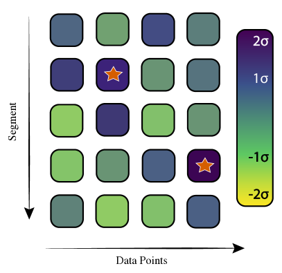
Figure 1: A schematic of the toy model data. Each row is a segment, consisting of four data points indicated by the rounded rectangles. The noise in the segments is drawn from a standard normal distribution, with its value indicated by the color scale of the rounded rectangle. Segments 2 and 4 from the top in this example contain a signal, added randomly to one of the four data points indicated by the vermilion star.

Using the p value from the pipelines as their detection statistics, we will calculate the joint likelihoods using a KDE as described in Sec. III. To do this we create a number of segments containing a signal to train a signal KDE, and similarly train a noise KDE using segments that do not contain a signal. Then for a simulation where $\Lambda_{\mathrm{s}}$ is unknown, we can score the outputs of the pipelines against the KDEs to perform a unified FGMC analysis using Eq. (14), and measure the noise and signal counts, $\Lambda_{\mathrm{n}}{}{}$ and $\Lambda_{\mathrm{s}}{}{}$.

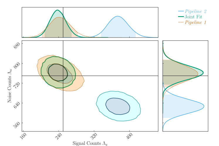
(a) Analysis with Pipeline 1 and Pipeline 2. The horizontal and vertical axes are the measured signal and noise count parameters. Pipeline 2 is clearly biased as it only uses the loudest data point of a segment for analysis, but the unified FGMC analysis performing a joint fit can correct for it.

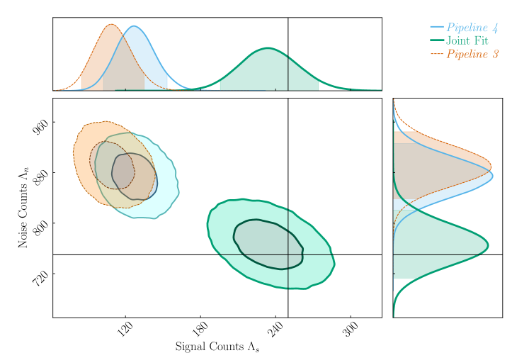
(b) Analysis with Pipeline 3 and Pipeline 4. While both pipelines only see half the simulated signals, the joint analysis learns to correct for this from the correlations in the joint signal distributions.

Figure 2: Toy-model exploration of the unified $p_{\mathrm{astro}}$ formalism. A signal value, $\lambda_{\mathrm{s}}=3$ was used in both cases. In both figures, the solid vertical and horizontal lines indicate the real number of segments with (and without) a signal. The shaded regions in the marginal plots are $90\%$ uncertainty levels while the two-dimensional contours correspond to 50% and 90% levels.

The algorithmic choices made by the pipelines mean that their results differ from each other, and can introduce a bias in their estimate of signal counts (and thereby $p_{\mathrm{astro}}$). For instance, consider Pipeline 3, which can only see about half of the total signals. When combining the output of the pipelines, the KDEs do not know a priori about these biases and will have to learn it from the triggers. In a joint analysis between Pipeline 3 and Pipeline 4, the signal KDE can learn that only about half the analyzed segments will have a low p value in Pipeline 3 (i.e., when a signal is added to the first two data points) and that these are the segments in which Pipeline 4 will likely give a high p value (and vice versa).

Figure 2 shows an FGMC analysis for two separate toy model analyses. In both Figs. 2(a) and 2(b), we separately simulated $1000$ segments of data with about a quarter ($\Lambda_{s}=250$) of the segments having a signal with $\lambda_{\mathrm{s}}=3$. Figure 2(a) shows the signal and noise counts estimated by Pipeline 1 and Pipeline 2, along with a unified fit. As expected, Pipeline 2 shows a bias in its recovery which nevertheless the joint analysis can correct for. Figure 2(b) shows the results of a toy-model analysis with Pipeline 3 and Pipeline 4. Both pipelines only see about half of the simulated signals, by design. However, the joint analysis learns this bias through the signal KDE and can account for it.

This section shows, using a simple example, how outputs from multiple pipelines can be combined using the unified formalism that we have developed. It also shows how certain kinds of biases can be corrected when multiple pipelines are joined together, by drawing information from the correlations (or lack thereof) between the outputs of the pipelines. These examples demonstrate the robustness of the unified $p_{\mathrm{astro}}$ method.

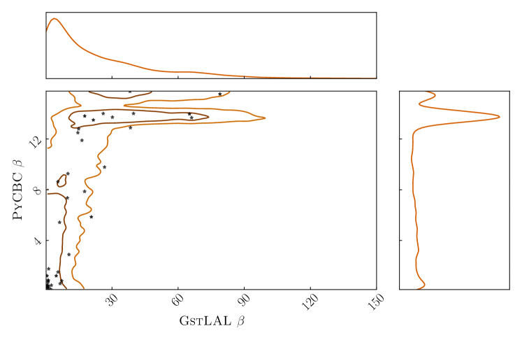
(a) The signal distribution $p(\vec{x}|\mathcal{S})$ learned using a KDE to the simulated signals that are commonly found by both GstLAL and PyCBC. The stars are the O3a on-source triggers from GWTC-2.1 found by both pipelines Abbott et al. (2021d). The upper cutoff of the PyCBC distribution that is visible in the plot comes from the fact that the pipeline places a limit on the FAR based on the number of time slides performed. This translates to a cutoff at $\beta\approx 15.76$ and results in a bump in the PyCBC distribution at these values of $\beta$.

(b) The noise distribution $p(\vec{x}|\varnothing)$ fit to a $2$-dimensional Gaussian to the common noise triggers. The stars are the O3a on-source triggers from GWTC-2.1 found by both pipelines Abbott et al. (2021d).

Figure 3: Joint likelihood distributions for the signal and noise hypothesis. The spans of the signal and noise distributions span are dissimilar. The signal distribution extends to much larger $\beta$ values than the noise distribution. The contours correspond to $50\%$ and $90\%$ levels in both plots.

Figure 4: The distribution of triggers that were found by one pipeline only. The top plot shows the noise and signal distribution of GstLAL, while the bottom plot shows the PyCBC distribution of triggers. The black stars are again the on-source O3a triggers from GWTC-2.1 that have only been found by the corresponding pipeline Abbott et al. (2021d).

V Application to GWTC-2.1

We now test the unified $p_{\mathrm{astro}}$ method with real GW triggers (henceforth on-source triggers) by applying this to O3a results from GWTC-2.1 Abbott et al. (2021e). GWTC-2.1 applies a preliminary cut of $\mathrm{FAR}\leq 2~{}\mathrm{day}^{-1}$, which we also adopt. While this analysis uses real data, it is only intended to be illustrative, and we adopt some simplifications for computational simplicity.

We use results from the GstLAL Messick et al. (2017); Sachdev et al. (2019); Cannon et al. (2021) and PyCBC Usman et al. (2016); Nitz et al. (2017); Davies et al. (2020) pipelines, and restrict ourselves to triggers that are at least Hanford-Livingston coincident (i.e., present in data from LIGO Hanford and Livingston at a minimum). GWTC-2.1 Abbott et al. (2021e) uses two versions of the PyCBC pipelines; referred to as PyCBC-broad and PyCBC-BBH; in this analysis we only use the former version, which we will simply refer to as PyCBC. While our formalism is general, we focus solely on CBC signals; a choice that is primarily driven by prudence, as we have only seen the population of CBC signals so far Abbott et al. (2021a). Furthermore, for the sake of simplicity we will only use BBH signals for the training; this will also serve as a test to see if the method can distinguish sufficiently between signal types and to test overfitting. These simplifications make it easier to illustrate the behavior of the unified $p_{\mathrm{astro}}$, and highlight the key considerations for an analysis to be performed for future GW catalogs.

We use pipeline settings that are as similar as possible to the runs in GWTC-2.1 Abbott et al. (2021e). A crucial factor to consider is that the search pipelines have to be run in a way that we can establish a one-to-one correspondence between their triggers so that we can learn the correlations between them. This is necessary even in the case where one pipeline registers a trigger and the other does not because the absence of the trigger is itself useful information. While one-to-one correspondence is straightforward for simulated signal triggers (described in Sec. V.1), it can be somewhat ambiguous to define in the case of noise triggers (implementation details are explained in Sec. V.2).

In order to calculate a unified $p_{\mathrm{astro}}$, Eq. (14), and Eq. (15) require us to construct the joint distribution of a statistic from each pipeline. We choose to use the FAR as the base statistic here as it is easily interpretable, commonly used by all pipelines and informative of the relative significance of triggers. However, the dynamic range of FARs can be large, and we therefore define a statistic $\beta$ that is related to the logarithm of the inverse FAR,

$$\beta(\mathrm{FAR})=\log\left(1+\frac{\kappa}{\mathrm{FAR}}\right),$$ (18)

where $\kappa$ is a scaling constant, which we set to a value of $\kappa=100~{}\mathrm{yr}^{-1}$. This number is set to give a good dynamic range to $\beta$ but our results are insensitive to its actual value. Higher values of $\beta$ correspond to more significant candidates.

We construct three cases each for the noise and signal hypotheses, corresponding to triggers that are registered (i) only by GstLAL, (ii) only by PyCBC, and (iii) by both pipelines. We find that separate modeling the three cases is necessary in order to achieve a faithful fit of signal triggers, which can cover a wide range on the $\beta$ space and show significant structure. In addition, this allows us to consider the case where one pipeline would not see a signal but the other does. For example, in the GWTC-2.1 analysis Abbott et al. (2021d), PyCBC did not assign FARs to events which triggered in a single detector (although this is now possible Davies and Harry (2022)), but GstLAL did. In the future, a more sophisticated fitting method like a convolutional neural network or a random forest classifier might make multiple separate fits unnecessary.

The distributions are usually normalized such that the total probability over its parameter space is one. Therefore, when considering multiple separate cases we need to renormalize them to account for the relative probability of the class they represent. We do this by multiplying the output of the distribution with the fraction of signal or noise triggers that fall in that particular class. We find that getting a joint trigger is $\approx 104$ times more likely under the signal hypothesis than the noise hypothesis. Meanwhile, a GstLAL-only (PyCBC-only) trigger is $\approx 2.77$ ($\approx 3.87$) times more likely under the noise hypothesis than the signal hypothesis. The numbers quoted correspond to triggers that pass a $2~{}\mathrm{day}^{-1}$ FAR threshold.

Figure 5: The posterior for the signal and noise counts in the joint analysis. The shaded region in the one-dimensional posterior corresponds to $90\%$ uncertainty levels, while the contours in the two-dimensional posteriors are the $50\%$ and $90\%$ levels. We recover a median value $\Lambda_{s}=53^{+10}_{-13}$.

V.1 Signal distribution

The signal distributed is generated by fitting simulated software signals or injections that are added to the detector noise, to a KDE. We use the same simulated signals as from the GWTC-3 analysis Collaboration et al. (2021), whose distribution is described in detail in Appendix C.7 (the injection row of Table X) of the GWTC-3 paper Abbott et al. (2021a). In particular, the source masses are distributed as

$$\begin{split}p(m_{1})&\propto m_{1}^{-2.35},\\ \quad p(m_{2}\,|\,m_{1})&\propto m_{2}.\end{split}$$ (19)

The redshift distribution is flat in comoving volume, with a maximum redshift of $1.9$, assuming a $\Lambda$CDM cosmology Ade et al. (2016). We restrict ourselves to injections with source-frame component masses $3M_{\odot}$–$100M_{\odot}$ to focus solely on BBHs. The simulated population is not a close match to the inferred astrophysical population Abbott et al. (2021b); Callister and Farr (2023). However, it shares broad characteristics and is simple to use. Therefore it suffices for our illustrative calculation. Using a population model that more closely resembles the underlying population should enable more accurate calculation of the true alarm rate, and hence $p_{\mathrm{astro}}$.

In any KDE-based analysis, the choice of the KDE bandwidth is important, especially for multidimensional distributions with intricate shapes. In our illustrative analysis, the bandwidth was picked manually by checking that the KDE approximates well the distribution of injections. We verified that the one-dimensional cumulative distributions of the KDE and the injection set match, and also cross-checked the KDE against a KDE using the Silverman rule of thumb Silverman (1986). Ultimately, a realistic application would need a more sophisticated fitting scheme, for example, KDEs fit using an iterative approach Sadiq et al. (2023) or a machine-learning approach such as using normalizing flows.

The top plot of Fig. 3(a) shows the joint distribution of signals that are found by both PyCBC and GstLAL, and Fig, 4 shows the distribution of signal triggers that are found only by one pipeline.

V.2 Noise distribution

The noise distribution is fit using data with a nonphysical time shift higher than the light travel time between detectors to remove correlations between any real signals. Generating this data is computationally expensive, therefore, in this proof-of-concept analysis, we use O3a data with a single time shift where LIGO Livingston and Virgo data streams were shifted by $0.62831$ and $0.31415~{}\mathrm{s}$, respectively, in relation to LIGO Hanford.

To define corresponding noise triggers between the pipelines, we match the times of the time-shifted triggers within a window of $1~{}\mathrm{s}$, comparable to the typical window used for grouping triggers in O3 Abbott et al. (2021a). This procedure gives us $256$ GstLAL triggers and $348$ PyCBC triggers that pass the FAR threshold of $2~{}\mathrm{day}^{-1}$; of these, only $12$ triggers are common between pipelines. For a unified $p_{\mathrm{astro}}$ analysis intended to be used in production of a GW catalog, a larger set of noise triggers would be required.

The small number of noise triggers common between the pipelines makes it difficult to accurately reconstruct the distribution. However, as our primary goal is to illustrate unified $p_{\mathrm{astro}}$ method, rather than to produce a full set of results, these triggers are sufficient for completing a demonstrative calculation. To make use of the small number of triggers that are common between the pipelines, we adopt a bootstrapping procedure to generate more triggers. To do this, we first fit triggers that pass a $10~{}\mathrm{day}^{-1}$ cut to a KDE, and draw $10^{4}$ triggers that pass a $2~{}\mathrm{day}^{-1}$ cut. This corresponds to doing $\approx 17$ time slides in total. To avoid overfitting the noise triggers, we choose to employ a truncated Gaussian fit to them, instead of a KDE. The assumption of a Gaussian is purely for simplicity, and a more careful choice of estimating the noise distribution would be needed for a proper analysis. The single-pipeline noise triggers are fit using a truncated Gaussian with mean $\mu=\beta(2~{}\mathrm{day}^{-1})$ and a standard deviation calculated from the noise triggers. The joint noise distribution is fit with a $2$-dimensional truncated Gaussian with $\mu=\beta(2~{}\mathrm{day}^{-1})$ and the covariance matrix calculated from the noise triggers. Figure 3(b) shows the distribution of joint triggers, while Fig. 4 shows the single-pipeline triggers in this bootstrapped data set.

The sparseness of noise triggers means that the noise distribution is not accurately reconstructed. This is liable to give biased values for $p_{\mathrm{astro}}$: where the noise likelihood is underestimated, $p_{\mathrm{astro}}$ will be underestimated, and where the noise likelihood is overestimated, $p_{\mathrm{astro}}$ will be underestimated. However, the goal of this application is to show that the unified $p_{\mathrm{astro}}$ formalism yields sensible results to illustrate what would be needed for future analyses. A realistic application of this process to GW data will likely require multiple time shifts or some other process to generate a larger number of high-fidelity noise triggers, and then a careful reconstruction of the shape of the noise distribution.

V.3 Computing a unified $p_{\mathrm{astro}}$

		GstLAL		PyCBC
GPS time	GW name	FAR $(\text{yr}^{-1})$	$\beta$	FAR $(\text{yr}^{-1})$	$\beta$	Unified $p_{\rm astro}$
$1238782700.0$	GW$190408\_181802$	$2.1\times 10^{-15}$	$38.4$	$2.5\times 10^{-04}$	$12.9$	$>0.99$
$1239082262.0$	GW$190412\_053044$	$1.9\times 10^{-27}$	$66.1$	$1.1\times 10^{-04}$	$13.7$	$>0.99$
$1240327333.0$	-	$9.1\times 10^{-01}$	$4.7$	$4.2\times 10^{+01}$	$1.2$	0.98
$1240944862.0$	GW$190503\_185404$	$2.3\times 10^{-06}$	$17.6$	$3.8\times 10^{-02}$	$7.9$	$>0.99$
$1241108686.0$	-	$1.7\times 10^{+01}$	$1.9$	-	-	0.85
$1241719652.0$	GW$190512\_180714$	$7.7\times 10^{-12}$	$30.2$	$1.1\times 10^{-04}$	$13.7$	$>0.99$
$1241816086.0$	GW$190513\_205428$	$1.3\times 10^{-05}$	$15.8$	-	-	$>0.99$
$1242107479.0$	GW$190517\_055101$	$4.5\times 10^{-03}$	$10.0$	$9.4\times 10^{-03}$	$9.3$	$>0.99$
$1242315362.0$	GW$190519\_153544$	$2.2\times 10^{-06}$	$17.6$	$1.0\times 10^{-04}$	$13.8$	$>0.99$
$1242442967.0$	GW$190521\_030229$	$2.0\times 10^{-01}$	$6.2$	$4.4\times 10^{-01}$	$5.4$	$>0.99$
$1242459857.0$	GW$190521\_074359$	$5.0\times 10^{-33}$	$79.0$	$1.8\times 10^{-05}$	$15.5$	$>0.99$
$1242984073.0$	GW$190527\_092055$	$2.3\times 10^{-01}$	$6.1$	-	-	$>0.99$
$1243533585.0$	GW$190602\_175927$	$1.1\times 10^{-07}$	$20.6$	$2.9\times 10^{-01}$	$5.9$	$>0.99$
$1243926576.0$	-	$1.2\times 10^{+01}$	$2.2$	$6.4\times 10^{+02}$	$0.1$	0.72
$1243985856.0$	-	$3.2\times 10^{+02}$	$0.3$	$2.6\times 10^{+02}$	$0.3$	0.59
$1245221073.0$	-	$1.2\times 10^{+02}$	$0.6$	$1.8\times 10^{+02}$	$0.4$	0.53
$1245874666.0$	-	$6.2\times 10^{+02}$	$0.1$	$2.2\times 10^{+02}$	$0.4$	0.80
$1246048404.0$	GW$190701\_203306$	$5.7\times 10^{-03}$	$9.8$	$6.4\times 10^{-02}$	$7.4$	$>0.99$
$1246385767.0$	-	$5.3\times 10^{+00}$	$3.0$	-	-	$>0.99$
$1246487219.0$	GW$190706\_222641$	$5.0\times 10^{-05}$	$14.5$	$3.7\times 10^{-04}$	$12.5$	$>0.99$
$1246779793.0$	-	$1.0\times 10^{+01}$	$2.4$	-	-	0.99
$1246849694.0$	-	$2.7\times 10^{+00}$	$3.6$	-	-	$>0.99$
$1247616534.0$	GW$190720\_000836$	$4.4\times 10^{-08}$	$21.5$	$1.4\times 10^{-04}$	$13.5$	$>0.99$
$1248242631.0$	GW$190727\_060333$	$2.7\times 10^{-10}$	$26.6$	$5.6\times 10^{-03}$	$9.8$	$>0.99$
$1248331528.0$	GW$190728\_064510$	$5.4\times 10^{-16}$	$39.8$	$8.2\times 10^{-05}$	$14.0$	$>0.99$
$1248617394.0$	GW$190731\_140936$	$3.3\times 10^{-01}$	$5.7$	-	-	$>0.99$
$1249479778.0$	-	$6.6\times 10^{+00}$	$2.8$	-	-	$>0.99$
$1250620378.0$	-	$5.2\times 10^{+00}$	$3.0$	-	-	$>0.99$
$1251009263.0$	GW$190828\_063405$	$5.0\times 10^{-27}$	$65.2$	$8.5\times 10^{-05}$	$14.0$	$>0.99$
$1251010527.0$	GW$190828\_065509$	$3.5\times 10^{-05}$	$14.9$	$2.8\times 10^{-04}$	$12.8$	$>0.99$
$1251588283.0$	-	$1.6\times 10^{+01}$	$2.0$	-	-	0.92
$1251926900.0$	-	$1.0\times 10^{+01}$	$2.4$	-	-	$>0.99$
$1252627040.0$	GW$190915\_235702$	$7.8\times 10^{-06}$	$16.4$	$6.8\times 10^{-04}$	$11.9$	$>0.99$
$1252699636.0$	GW$190916\_200658$	$1.2\times 10^{+01}$	$2.2$	-	-	0.99
$1252756008.0$	GW$190917\_114630$	$6.6\times 10^{-01}$	$5.0$	-	-	$>0.99$
$1252939489.0$	-	$9.0\times 10^{+00}$	$2.5$	-	-	$>0.99$
$1252987339.0$	-	$5.1\times 10^{+01}$	$1.1$	$8.0\times 10^{+01}$	$0.8$	0.65
$1253326744.0$	GW$190924\_021846$	$5.0\times 10^{-10}$	$26.0$	$8.2\times 10^{-05}$	$14.0$	$>0.99$
$1253509434.0$	GW$190926\_050336$	$1.1\times 10^{+00}$	$4.5$	-	-	$>0.99$
$1253755327.0$	GW$190929\_012149$	$1.5\times 10^{-01}$	$6.5$	$1.2\times 10^{+02}$	$0.6$	$>0.99$
$1253885759.0$	GW$190930\_133541$	$4.3\times 10^{-01}$	$5.5$	$1.8\times 10^{-02}$	$8.6$	$>0.99$

Table 1: Triggers with a unified $p_{\mathrm{astro}}{}\geq 0.5$ from our illustrative analysis. The triggers that have $p_{\mathrm{astro}}{}{}\geq 0.5$ in at least one pipeline in GWTC-2.1 Abbott et al. (2021d) are shown in the second column. Also listed are the FARs of the triggers from the GstLAL and PyCBC pipelines. The GW name of the triggers also recovered with $p_{\mathrm{astro}}$$\geq 0.5$ by at least one pipeline in GWTC-2.1 is given in the second column. These results illustrate the properties of the unified $p_{\mathrm{astro}}$ method, but a larger number of noise triggers, and more accurate population models, would be needed to obtain reliable quantitative results.

After restricting ourselves to ones that are at least Hanford-Livingston coincident, and have been found by at least one of GstLAL or PyCBC, we are left with $553$ on-source triggers from the GWTC-2.1 O3a results Abbott et al. (2021a). Using the signal and noise models described above, we can now proceed to calculate a unified $p_{\mathrm{astro}}$ for these triggers.

First, through Eq. (10), we estimate $\Lambda_{\mathrm{s}}{}{}$ and $\Lambda_{\mathrm{n}}{}{}$ for the joint analysis. We do this using the Markov-chain Monte Carlo sampler emcee Foreman-Mackey et al. (2013). We use uniform priors on the count parameters, $\Lambda_{\mathrm{s}}{}{}\in[0,1000]$ and $\Lambda_{\mathrm{n}}{}{}\in[0,1000]$. The triggers are then scored against the appropriate distribution to calculate $p({x_{i}}|\mathcal{S})$ and $p({x_{i}}|\varnothing)$.

Figure 5 shows the posterior distribution of $\Lambda_{\mathrm{s}}{}{}$ and $\Lambda_{\mathrm{n}}{}{}$, with a median $\Lambda_{\mathrm{s}}{}{}$ of $53$. Table 1 lists the $41$ triggers that have unified $p_{\mathrm{astro}}{}\geq 0.5$. Most triggers are reported by both GstLAL and PyCBC, but we do have a few triggers that are detected by GstLAL alone, which corresponds to the high $\beta$ tail of the on-source triggers in the top panel of Fig. 4. This is qualitatively consistent with the $44$ triggers found with a $p_{\mathrm{astro}}{}\geq 0.5$ by at least one pipeline in GWTC-2.1 analysis Abbott et al. (2021a).

In Table 1, we recover $26$ triggers that are also reported with $p_{\mathrm{astro}}{}{}>0.5$ in at least one search pipeline in the GWTC-2.1 analysis Abbott et al. (2021a) (the corresponding GW identification of these triggers has been given for easy identification) while the remaining $15$ triggers were below this threshold. Inspecting the $\beta$ values of these triggers show that they are usually low, and comparing with the noise distributions, it is plausible that they could be consistent with noise if some of the modeling assumptions are relaxed. The simplified modeling of the noise distribution is expected to lead to the promotion of some noise triggers while suppressing some real signals.

		GstLAL		PyCBC
GPS time	GW name	FAR $(\text{yr}^{-1})$	$\beta$	FAR $(\text{yr}^{-1})$	$\beta$	Unified $p_{\rm astro}$
$1239917954.0$	GW$190421\_213856$	$2.8\times 10^{-03}$	$10.5$	$5.9\times 10^{+00}$	$2.9$	$<0.01$
$1246527224.0$	GW$190707\_093326$	$2.7\times 10^{-15}$	$38.2$	$9.7\times 10^{-06}$	$16.1$	$<0.01$
$1248834439.0$	GW$190803\_022701$	$7.3\times 10^{-02}$	$7.2$	$8.1\times 10^{+01}$	$0.8$	$<0.01$

Table 2: Triggers with a unified $p_{\mathrm{astro}}{}<0.5$ in our illustrative analysis, but with a $p_{\mathrm{astro}}{}\geq 0.5$ in either GstLAL or PyCBC in GWTC-2.1 Abbott et al. (2021d)

In the case of joint triggers there is a heavy weight in favor of signal triggers as discussed in Sec. V. The exact quantitative results might be susceptible to small-number statistics, and it is plausible that some of these would be down weighted if we had a more complete noise distribution from more time slides. However, the results show the expected behavior that having multiple pipelines find a candidate when their noise distributions are largely uncorrelated, increases our certainty that a candidate is real.

In Table 2, we show the list of triggers with a unified $p_{\mathrm{astro}}{}{}<0.5$, but with a $p_{\mathrm{astro}}{}{}\geq 0.5$ in either GstLAL or PyCBC in GWTC-2.1 Abbott et al. (2021d). While the correlation between pipelines increases $p_{\mathrm{astro}}$ for some candidates, the unified analysis also down-weights certain triggers, in particular those with highly asymmetric $\beta$ values. This is because the joint simulated-signal trigger distribution has a strong correlation between the $\beta$ (and thereby the FAR) values of two pipelines; this is expected since both are matched filter pipelines using CBC templates. For example, GW190803_022701 has GstLAL and PyCBC FARs of $7.3\times 10^{-2}~{}\mathrm{yr}^{-1}$ and $81~{}\mathrm{yr}^{-1}$, respectively. Therefore, while the GstLAL significance of the trigger is high, the asymmetric FARs in the two pipelines gives it a lower weight in the unified analysis. In our case, the low $p_{\mathrm{astro}}$ can potentially be explained by the choice of a Gaussian for the noise distribution with heavy tails at large $\beta$. The uncertainties involved in the noise and the signal distributions in this illustrative analysis, and the fact that we do not include other search pipelines, mean that we should not rule out the triggers in Table 2. Nevertheless, the results demonstrate that there is information that is uniquely captured by a joint analysis of multiple pipelines. In practice, we would expect that any high-significance candidate that is a clear outlier in the signal distribution would warrant further investigation to understand why the pipelines differ in their response.

Finally, many of the triggers in Table 1 have a $p_{\mathrm{astro}}$ close to $1$. This is likely an overestimate, due to the sparseness of the noise distribution which can lead to an artificially low noise likelihood in Eq. (15). We equally expect that some of the low-probability candidates, not shown in the table, have underestimated $p_{\mathrm{astro}}$ for the same reason. The specific values we get are also dependent on the strong modeling assumptions made for the noise distribution. A more realistic analysis would probably require adequate non-parametric modeling of the noise distribution such that any structure in the parameter space can be identified. While it is worth bearing these limitations in mind, both Table 1 and Fig. 5 qualitatively demonstrate consistency of the results with GWTC-2.1, indicating that even with simpler modeling choices this method can yield sensible overall results.

VI Discussion and conclusion

We have developed a statistical formalism for combining information from multiple search pipelines to calculate a unified $p_{\mathrm{astro}}$. We first demonstrated this formalism using a simple toy model, showing that it can consistently combine information and even account for biases in search pipelines. We then applied the framework to O3a data, using triggers from GstLAL and PyCBC, demonstrating how correlations between pipelines may update our understanding of candidates, but highlighting the importance of using accurate models for the signal and noise populations.

Currently, multiple search pipelines are used to identify interesting candidates, each with its own strengths. A unified $p_{\mathrm{astro}}$ can potentially reduce confusion in the interpretation of triggers found by different pipelines and can help in using marginal triggers for subsequent GW analyses. We have shown that certain types of correlations between pipelines can inform the significance that the unified analysis assigns to a trigger. Similarly, combining the search pipelines’ results mitigates the need to calculate an effective trials factor to correct the individual-pipeline FARs to account for repeated analysis of the same data. Calculating this trials factor is generally nontrivial. Our formalism can naturally and consistently account for these considerations since it calculates how triggers in one pipeline are correlated with those in another pipeline.

While we have demonstrated that this method can estimate signal and noise counts, and a unified $p_{\mathrm{astro}}$ in a sensible and consistent manner, the paucity of noise triggers is a clear computational bottleneck. The scarcity of these triggers can be understood by considering the FAR thresholds used. The $2~{}\mathrm{day}^{-1}$ threshold used means that we will be limited to a few hundred noise triggers in each pipeline per a six month run. Therefore, depending on the structure in the joint noise correlations, we would probably need $\mathcal{O}(10$–$100)$ time slides to obtain an accurate representation of the noise distribution. The number of noise triggers that are common between pipelines will be only a fraction of the total number of noise triggers, and if the noise backgrounds are distinct, then there will only be a small fraction in common. This may indicate a need for multiple coordinated time shifts between pipelines to build up the noise distribution. One can also consider other methods of building noise distributions such as modeling the joint noise distribution and drawing from it, similar in philosophy to the GstLAL pipeline Cannon et al. (2013).

However, while the low number of common noise triggers does pose a difficulty for reconstructing the shape of the noise distribution, it also highlights the importance of considering the number of candidates in common between pipelines: if common noise triggers are rare, but common signal triggers are frequent, then a candidate being found by multiple pipelines should increase its $p_{\mathrm{astro}}$. We already see this in the analysis done here where a joint trigger is about $100$ times more likely under the signal hypothesis.

If suitable data products (injection sets and noise triggers) are available, this formalism can be readily applied to include other search pipelines, notably those used by the LVK such as MBTA Adams et al. (2016); Aubin et al. (2021) and cWB Klimenko and Mitselmakher (2004); Klimenko et al. (2011, 2016), as well as pipelines developed for external analysis of public data Venumadhav et al. (2019). This would enable the construction of a single GW catalog accounting for all analyses. A strength of this formalism when constructing joint catalogs is that it would differentially weigh search pipelines, depending on their precision and accuracy by taking into account the shape of the joint simulated-signal distribution. Hence, as long as the simulated-signal distribution sufficiently reflects the true distribution of GW sources, it should be possible to correct for pipelines missing signals over some region of parameter space, or producing spurious triggers in another.

The addition of cWB (and other minimally modeled pipelines Lynch et al. (2017); Kanner et al. (2016)) to catalog production could be extremely useful, as it can be sensitive in regions of the CBC parameter space where modeled searches do not perform well, such as eccentric binaries Abbott et al. (2019b), in addition to non-CBC transient sources. The sensitivity to non-CBC sources is a complication for current analyses, as the $p_{\mathrm{astro}}$ calculations are done assuming only CBC sources (discussed in Appendix F of the GWTC-3 paper Abbott et al. (2021c)). Non-CBC source have a lower true alarm rate than CBC sources, and hence a lower $p_{\mathrm{astro}}$ at a given FAR; consequently, misidentifying a trigger as CBC will lead to an overestimate of its $p_{\mathrm{astro}}$. To mitigate this, LVK analyses have imposed an additional criterion for cWB candidates, that they must have a counterpart trigger from a template-based CBC pipeline Abbott et al. (2019a, 2021a). This is effectively an approximation to the unified $p_{\mathrm{astro}}$ framework, acknowledging that for real CBC signals there would probably be correlation between pipeline results. This could be put on a more rigorous basis by explicitly using out unified $p_{\mathrm{astro}}$ framework, considering the response of the pipelines to simulated CBC and non-CBC signals.

Addition of more pipelines can make the problem of noise triggers more acute, as the number of triggers that are common between three or more pipelines might be small and extrapolation difficult. However, it is probable that noise triggers in a multiple-pipeline space would be so rare that we can conservatively set the noise likelihood to a small limiting value for such a case.

In this paper, we have only considered the simplest case of calculating a unified $p_{\mathrm{astro}}$. In a future work, we will extend it to implement binning in the mass space to estimate the astrophysical probability that a system is a BBH, a BNS or a neutron star–black hole binary (NSBH) Kapadia et al. (2020). Such an extension is in principle straightforward, where in addition to a statistic like the FAR we also fit distribution of recovered template chirp masses for simulated BBH, BNS and NSBH signal. On-source triggers can then be scored against such two-dimensional distributions to give the corresponding likelihood. Searches are often optimized in different ways giving them differential sensitivity in specific parts of the mass space (e.g., PyCBC has an analysis tuned to BBHs Nitz et al. (2020); Abbott et al. (2021c)). Calculating unified probabilities in conjugation with mass binning will allow us to fold in this differential sensitivity in a consistent, unbiased way in a way akin to the toy model example with Pipeline 3 and Pipeline 4 in Sec. IV.

A key uncertainty in the calculation of $p_{\mathrm{astro}}$ is the form of the underlying source population. Errors in the assumed population translate to a misestimation of the true alarm rate, and hence $p_{\mathrm{astro}}$. A way to mitigate this would be to infer the population simultaneously while calculating $p_{\mathrm{astro}}$ Gaebel et al. (2019); Galaudage et al. (2020); Roulet et al. (2020). This additionally enables lower-significance candidates to be used in population inference. Using a unified $p_{\mathrm{astro}}$ makes it easier to assess the contamination fraction in a catalog based upon several pipelines, and hence would make it more convenient to perform such joint inference in the future.

While we have only considered the application of our method to final search analyses performed offline, an extension to low-latency detections is also theoretically possible. By combining multiple pipelines we depend less on one pipeline and hence should be less susceptible to incorrect alerts and retractions. In combination with mass binning, this could be extremely useful for electromagnetic follow-up of GW candidates Lynch et al. (2018). Since many such follow-ups are often target-of-opportunity observations, improving the reliability of trigger information can be valuable in evaluating the proper usage of scarce telescope time. The relative scarcity of noise triggers could be a bigger computational issue in low latency, as the joint noise distributions will have to be continuously reevaluated at a reasonable cadence in order to account for the changing detector state Buikema et al. (2020); Acernese et al. (2022). Therefore, further work would be needed to identify methods that could potentially be used to reconstruct the noise distribution in low latency.

Finally, Bayesian frameworks have been developed to assess the probability of multimessenger detections Ashton et al. (2018); Bartos et al. (2019); Veske et al. (2021); Piotrzkowski et al. (2022). These calculate the probabilities associated with candidates being background noise or astrophysical signals from different sources or the same source. Our unified $p_{\mathrm{astro}}$ framework naturally feeds into these calculations. Furthermore, our framework would enable the extension of these calculations to consider how a nondetection in one messenger impacts the probability that a candidate in a counterpart messenger is real. Given the rich science that may result from a multimessenger discovery Abbott et al. (2017c, 2020a); Margutti and Chornock (2021), this may be a valuable avenue of future investigation.

The data used in this paper for the analysis of GWTC-2.1 triggers is available as a Zenodo repository zen .

References

- Abbott et al. (2016a) B. P. Abbott et al. (LIGO Scientific, Virgo), “Observation of Gravitational Waves from a Binary Black Hole Merger,” Phys. Rev. Lett. 116, 061102 (2016a), arXiv:1602.03837 [gr-qc] .
- Abbott et al. (2021a) R. Abbott et al. (LIGO Scientific, Virgo, KAGRA), “GWTC-3: Compact Binary Coalescences Observed by LIGO and Virgo During the Second Part of the Third Observing Run,” (2021a), arXiv:2111.03606 [gr-qc] .
- Aasi et al. (2015) J. Aasi et al. (LIGO Scientific), “Advanced LIGO,” Class. Quant. Grav. 32, 074001 (2015), arXiv:1411.4547 [gr-qc] .
- Acernese et al. (2015) F. Acernese et al. (Virgo), “Advanced Virgo: a second-generation interferometric gravitational wave detector,” Class. Quant. Grav. 32, 024001 (2015), arXiv:1408.3978 [gr-qc] .
- Pitkin et al. (2011) Matthew Pitkin, Stuart Reid, Sheila Rowan, and Jim Hough, “Gravitational Wave Detection by Interferometry (Ground and Space),” Living Rev. Rel. 14, 5 (2011), arXiv:1102.3355 [astro-ph.IM] .
- Abbott et al. (2020a) B. P. Abbott et al. (KAGRA, LIGO Scientific, Virgo), “Prospects for observing and localizing gravitational-wave transients with Advanced LIGO, Advanced Virgo and KAGRA,” Living Rev. Rel. 23, 3 (2020a), arXiv:1304.0670 [gr-qc] .
- Abbott et al. (2020b) Benjamin P Abbott et al. (LIGO Scientific, Virgo), “A guide to LIGO–Virgo detector noise and extraction of transient gravitational-wave signals,” Class. Quant. Grav. 37, 055002 (2020b), arXiv:1908.11170 [gr-qc] .
- Abbott et al. (2016b) B. P. Abbott et al. (LIGO Scientific, Virgo), “GW150914: First results from the search for binary black hole coalescence with Advanced LIGO,” Phys. Rev. D 93, 122003 (2016b), arXiv:1602.03839 [gr-qc] .
- Abbott et al. (2016c) B. P. Abbott et al. (LIGO Scientific, Virgo), “Observing gravitational-wave transient GW150914 with minimal assumptions,” Phys. Rev. D 93, 122004 (2016c), [Addendum: Phys.Rev.D 94, 069903 (2016)], arXiv:1602.03843 [gr-qc] .
- Farr et al. (2015) Will M. Farr, Jonathan R. Gair, Ilya Mandel, and Curt Cutler, “Counting And Confusion: Bayesian Rate Estimation With Multiple Populations,” Phys. Rev. D 91, 023005 (2015), arXiv:1302.5341 [astro-ph.IM] .
- Guglielmetti et al. (2009) F. Guglielmetti, R. Fischer, and V. Dose, “Background-Source Separation in astronomical images with Bayesian probability theory (I): the method,” Mon. Not. Roy. Astron. Soc. 396, 165 (2009), arXiv:0903.2342 [astro-ph.IM] .
- Abbott et al. (2016d) B. P. Abbott et al. (LIGO Scientific, Virgo), “The Rate of Binary Black Hole Mergers Inferred from Advanced LIGO Observations Surrounding GW150914,” Astrophys. J. Lett. 833, L1 (2016d), arXiv:1602.03842 [astro-ph.HE] .
- Abbott et al. (2016e) B. P. Abbott et al. (LIGO Scientific, Virgo), “Supplement: The Rate of Binary Black Hole Mergers Inferred from Advanced LIGO Observations Surrounding GW150914,” Astrophys. J. Suppl. 227, 14 (2016e), arXiv:1606.03939 [astro-ph.HE] .
- Abbott et al. (2019a) B. P. Abbott et al. (LIGO Scientific, Virgo), “GWTC-1: A Gravitational-Wave Transient Catalog of Compact Binary Mergers Observed by LIGO and Virgo during the First and Second Observing Runs,” Phys. Rev. X 9, 031040 (2019a), arXiv:1811.12907 [astro-ph.HE] .
- Abbott et al. (2021b) R. Abbott et al. (LIGO Scientific, Virgo, KAGRA), “The population of merging compact binaries inferred using gravitational waves through GWTC-3,” (2021b), arXiv:2111.03634 [astro-ph.HE] .
- Nitz et al. (2021a) Alexander H. Nitz, Sumit Kumar, Yi-Fan Wang, Shilpa Kastha, Shichao Wu, Marlin Schäfer, Rahul Dhurkunde, and Collin D. Capano, “4-OGC: Catalog of gravitational waves from compact-binary mergers,” (2021a), arXiv:2112.06878 [astro-ph.HE] .
- Olsen et al. (2022) Seth Olsen, Tejaswi Venumadhav, Jonathan Mushkin, Javier Roulet, Barak Zackay, and Matias Zaldarriaga, “New binary black hole mergers in the LIGO-Virgo O3a data,” Phys. Rev. D 106, 043009 (2022), arXiv:2201.02252 [astro-ph.HE] .
- Abbott et al. (2021c) R. Abbott et al. (LIGO Scientific, Virgo), “GWTC-2: Compact Binary Coalescences Observed by LIGO and Virgo During the First Half of the Third Observing Run,” Phys. Rev. X 11, 021053 (2021c), arXiv:2010.14527 [gr-qc] .
- Abbott et al. (2021d) R. Abbott et al. (LIGO Scientific, Virgo), “GWTC-2.1: Deep Extended Catalog of Compact Binary Coalescences Observed by LIGO and Virgo During the First Half of the Third Observing Run,” (2021d), arXiv:2108.01045 [gr-qc] .
- Abbott et al. (2017a) B. P. Abbott et al. (LIGO Scientific, Virgo), “GW170817: Observation of Gravitational Waves from a Binary Neutron Star Inspiral,” Phys. Rev. Lett. 119, 161101 (2017a), arXiv:1710.05832 [gr-qc] .
- Abbott et al. (2021e) R. Abbott et al. (LIGO Scientific, KAGRA, Virgo), “Observation of Gravitational Waves from Two Neutron Star–Black Hole Coalescences,” Astrophys. J. Lett. 915, L5 (2021e), arXiv:2106.15163 [astro-ph.HE] .
- Buikema et al. (2020) Aaron Buikema et al. (aLIGO), “Sensitivity and performance of the Advanced LIGO detectors in the third observing run,” Phys. Rev. D 102, 062003 (2020), arXiv:2008.01301 [astro-ph.IM] .
- Acernese et al. (2022) F. Acernese et al. (Virgo), “The Virgo O3 run and the impact of the environment,” Class. Quant. Grav. 39, 235009 (2022), arXiv:2203.04014 [gr-qc] .
- Abbott et al. (2016f) B. P. Abbott et al. (LIGO Scientific, Virgo), “GW150914: The Advanced LIGO Detectors in the Era of First Discoveries,” Phys. Rev. Lett. 116, 131103 (2016f), arXiv:1602.03838 [gr-qc] .
- Kapadia et al. (2020) Shasvath J. Kapadia et al., “A self-consistent method to estimate the rate of compact binary coalescences with a Poisson mixture model,” Class. Quant. Grav. 37, 045007 (2020), arXiv:1903.06881 [astro-ph.HE] .
- Messick et al. (2017) Cody Messick et al., “Analysis Framework for the Prompt Discovery of Compact Binary Mergers in Gravitational-wave Data,” Phys. Rev. D 95, 042001 (2017), arXiv:1604.04324 [astro-ph.IM] .
- Sachdev et al. (2019) Surabhi Sachdev et al., “The GstLAL Search Analysis Methods for Compact Binary Mergers in Advanced LIGO’s Second and Advanced Virgo’s First Observing Runs,” (2019), arXiv:1901.08580 [gr-qc] .
- Hanna et al. (2020) Chad Hanna et al., “Fast evaluation of multidetector consistency for real-time gravitational wave searches,” Phys. Rev. D 101, 022003 (2020), arXiv:1901.02227 [gr-qc] .
- Cannon et al. (2021) Kipp Cannon et al., “GstLAL: A software framework for gravitational wave discovery,” SoftwareX 14, 100680 (2021), arXiv:2010.05082 [astro-ph.IM] .
- Allen et al. (2012) Bruce Allen, Warren G. Anderson, Patrick R. Brady, Duncan A. Brown, and Jolien D. E. Creighton, “FINDCHIRP: An Algorithm for detection of gravitational waves from inspiraling compact binaries,” Phys. Rev. D 85, 122006 (2012), arXiv:gr-qc/0509116 .
- Dal Canton et al. (2014) Tito Dal Canton et al., “Implementing a search for aligned-spin neutron star-black hole systems with advanced ground based gravitational wave detectors,” Phys. Rev. D 90, 082004 (2014), arXiv:1405.6731 [gr-qc] .
- Usman et al. (2016) Samantha A. Usman et al., “The PyCBC search for gravitational waves from compact binary coalescence,” Class. Quant. Grav. 33, 215004 (2016), arXiv:1508.02357 [gr-qc] .
- Nitz et al. (2017) Alexander H. Nitz, Thomas Dent, Tito Dal Canton, Stephen Fairhurst, and Duncan A. Brown, “Detecting binary compact-object mergers with gravitational waves: Understanding and Improving the sensitivity of the PyCBC search,” Astrophys. J. 849, 118 (2017), arXiv:1705.01513 [gr-qc] .
- Davies et al. (2020) Gareth S. Davies, Thomas Dent, Márton Tápai, Ian Harry, Connor McIsaac, and Alexander H. Nitz, “Extending the PyCBC search for gravitational waves from compact binary mergers to a global network,” Phys. Rev. D 102, 022004 (2020), arXiv:2002.08291 [astro-ph.HE] .
- (35) Tom Dent, “Technical note: Extending the pycbc pastro calculation to a global network,” .
- Adams et al. (2016) T. Adams, D. Buskulic, V. Germain, G. M. Guidi, F. Marion, M. Montani, B. Mours, F. Piergiovanni, and G. Wang, “Low-latency analysis pipeline for compact binary coalescences in the advanced gravitational wave detector era,” Class. Quant. Grav. 33, 175012 (2016), arXiv:1512.02864 [gr-qc] .
- Aubin et al. (2021) F. Aubin et al., “The MBTA pipeline for detecting compact binary coalescences in the third LIGO–Virgo observing run,” Class. Quant. Grav. 38, 095004 (2021), arXiv:2012.11512 [gr-qc] .
- Andres et al. (2022) Nicolas Andres et al., “Assessing the compact-binary merger candidates reported by the MBTA pipeline in the LIGO–Virgo O3 run: probability of astrophysical origin, classification, and associated uncertainties,” Class. Quant. Grav. 39, 055002 (2022), arXiv:2110.10997 [gr-qc] .
- Klimenko and Mitselmakher (2004) Sergey Klimenko and Guenakh Mitselmakher, “A wavelet method for detection of gravitational wave bursts,” Classical and Quantum Gravity 21, S1819 (2004).
- Klimenko et al. (2011) S. Klimenko, G. Vedovato, M. Drago, G. Mazzolo, G. Mitselmakher, C. Pankow, G. Prodi, V. Re, F. Salemi, and I. Yakushin, “Localization of gravitational wave sources with networks of advanced detectors,” Phys. Rev. D 83, 102001 (2011), arXiv:1101.5408 [astro-ph.IM] .
- Klimenko et al. (2016) S. Klimenko et al., “Method for detection and reconstruction of gravitational wave transients with networks of advanced detectors,” Phys. Rev. D 93, 042004 (2016), arXiv:1511.05999 [gr-qc] .
- Sutton (2009) Patrick J. Sutton, “Upper Limits from Counting Experiments with Multiple Pipelines,” Class. Quant. Grav. 26, 245007 (2009), arXiv:0905.4089 [physics.data-an] .
- Biswas et al. (2012) Rahul Biswas et al., “Detecting transient gravitational waves in non-Gaussian noise with partially redundant analysis methods,” Phys. Rev. D 85, 122009 (2012), arXiv:1201.2964 [gr-qc] .
- Galaudage et al. (2020) Shanika Galaudage, Colm Talbot, and Eric Thrane, “Gravitational-wave inference in the catalog era: evolving priors and marginal events,” Phys. Rev. D 102, 083026 (2020), arXiv:1912.09708 [astro-ph.HE] .
- Roulet et al. (2020) Javier Roulet, Tejaswi Venumadhav, Barak Zackay, Liang Dai, and Matias Zaldarriaga, “Binary Black Hole Mergers from LIGO/Virgo O1 and O2: Population Inference Combining Confident and Marginal Events,” Phys. Rev. D 102, 123022 (2020), arXiv:2008.07014 [astro-ph.HE] .
- Babak et al. (2013) S. Babak et al., “Searching for gravitational waves from binary coalescence,” Phys. Rev. D 87, 024033 (2013), arXiv:1208.3491 [gr-qc] .
- Cannon et al. (2013) Kipp Cannon, Chad Hanna, and Drew Keppel, “Method to estimate the significance of coincident gravitational-wave observations from compact binary coalescence,” Phys. Rev. D 88, 024025 (2013), arXiv:1209.0718 [gr-qc] .
- Venumadhav et al. (2020) Tejaswi Venumadhav, Barak Zackay, Javier Roulet, Liang Dai, and Matias Zaldarriaga, “New binary black hole mergers in the second observing run of Advanced LIGO and Advanced Virgo,” Phys. Rev. D 101, 083030 (2020), arXiv:1904.07214 [astro-ph.HE] .
- Nitz et al. (2020) Alexander H. Nitz, Thomas Dent, Gareth S. Davies, Sumit Kumar, Collin D. Capano, Ian Harry, Simone Mozzon, Laura Nuttall, Andrew Lundgren, and Márton Tápai, “2-OGC: Open Gravitational-wave Catalog of binary mergers from analysis of public Advanced LIGO and Virgo data,” Astrophys. J. 891, 123 (2020), arXiv:1910.05331 [astro-ph.HE] .
- Nitz et al. (2021b) Alexander H. Nitz, Collin D. Capano, Sumit Kumar, Yi-Fan Wang, Shilpa Kastha, Marlin Schäfer, Rahul Dhurkunde, and Miriam Cabero, “3-OGC: Catalog of Gravitational Waves from Compact-binary Mergers,” Astrophys. J. 922, 76 (2021b), arXiv:2105.09151 [astro-ph.HE] .
- Abbott et al. (2017b) Benjamin P. Abbott et al. (LIGO Scientific, Virgo), “Search for intermediate mass black hole binaries in the first observing run of Advanced LIGO,” Phys. Rev. D 96, 022001 (2017b), arXiv:1704.04628 [gr-qc] .
- Abbott et al. (2022) Rich Abbott et al. (LIGO Scientific, Virgo, KAGRA), “Search for intermediate-mass black hole binaries in the third observing run of Advanced LIGO and Advanced Virgo,” Astron. Astrophys. 659, A84 (2022), arXiv:2105.15120 [astro-ph.HE] .
- Pedregosa et al. (2011) F. Pedregosa, G. Varoquaux, A. Gramfort, V. Michel, B. Thirion, O. Grisel, M. Blondel, P. Prettenhofer, R. Weiss, V. Dubourg, J. Vanderplas, A. Passos, D. Cournapeau, M. Brucher, M. Perrot, and E. Duchesnay, “Scikit-learn: Machine learning in Python,” Journal of Machine Learning Research 12, 2825–2830 (2011).
- Davies and Harry (2022) Gareth S. Cabourn Davies and Ian W. Harry, “Establishing significance of gravitational-wave signals from a single observatory in the PyCBC offline search,” Class. Quant. Grav. 39, 215012 (2022), arXiv:2203.08545 [gr-qc] .
- Collaboration et al. (2021) LIGO Scientific Collaboration, Virgo Collaboration, and KAGRA Collaboration, “GWTC-3: Compact Binary Coalescences Observed by LIGO and Virgo During the Second Part of the Third Observing Run — O3 search sensitivity estimates,” (2021).
- Ade et al. (2016) P. A. R. Ade et al. (Planck), “Planck 2015 results. XIII. Cosmological parameters,” Astron. Astrophys. 594, A13 (2016), arXiv:1502.01589 [astro-ph.CO] .
- Callister and Farr (2023) Thomas A. Callister and Will M. Farr, “A Parameter-Free Tour of the Binary Black Hole Population,” (2023), arXiv:2302.07289 [astro-ph.HE] .
- Silverman (1986) B.W. Silverman, Density Estimation for Statistics and Data Analysis, Chapman & Hall/CRC Monographs on Statistics & Applied Probability (Taylor & Francis, 1986).
- Sadiq et al. (2023) Jam Sadiq, Thomas Dent, and Mark Gieles, “Binary vision: The merging black hole binary mass distribution via iterative density estimation,” (2023), arXiv:2307.12092 [astro-ph.HE] .
- Foreman-Mackey et al. (2013) Daniel Foreman-Mackey, David W. Hogg, Dustin Lang, and Jonathan Goodman, “emcee: The mcmc hammer,” Publications of the Astronomical Society of the Pacific 125, 306 (2013).
- Venumadhav et al. (2019) Tejaswi Venumadhav, Barak Zackay, Javier Roulet, Liang Dai, and Matias Zaldarriaga, “New search pipeline for compact binary mergers: Results for binary black holes in the first observing run of Advanced LIGO,” Phys. Rev. D 100, 023011 (2019), arXiv:1902.10341 [astro-ph.IM] .
- Lynch et al. (2017) Ryan Lynch, Salvatore Vitale, Reed Essick, Erik Katsavounidis, and Florent Robinet, “Information-theoretic approach to the gravitational-wave burst detection problem,” Phys. Rev. D 95, 104046 (2017), arXiv:1511.05955 [gr-qc] .
- Kanner et al. (2016) Jonah B. Kanner, Tyson B. Littenberg, Neil Cornish, Meg Millhouse, Enia Xhakaj, Francesco Salemi, Marco Drago, Gabriele Vedovato, and Sergey Klimenko, “Leveraging waveform complexity for confident detection of gravitational waves,” Phys. Rev. D 93, 022002 (2016), arXiv:1509.06423 [astro-ph.IM] .
- Abbott et al. (2019b) B. P. Abbott et al. (LIGO Scientific, Virgo), “Search for Eccentric Binary Black Hole Mergers with Advanced LIGO and Advanced Virgo during their First and Second Observing Runs,” Astrophys. J. 883, 149 (2019b), arXiv:1907.09384 [astro-ph.HE] .
- Gaebel et al. (2019) Sebastian M. Gaebel, John Veitch, Thomas Dent, and Will M. Farr, “Digging the population of compact binary mergers out of the noise,” Mon. Not. Roy. Astron. Soc. 484, 4008–4023 (2019), arXiv:1809.03815 [astro-ph.IM] .
- Lynch et al. (2018) Ryan Lynch, Michael Coughlin, Salvatore Vitale, Christopher W. Stubbs, and Erik Katsavounidis, “Observational implications of lowering the LIGO-Virgo alert threshold,” Astrophys. J. Lett. 861, L24 (2018), arXiv:1803.02880 [astro-ph.HE] .
- Ashton et al. (2018) G. Ashton, E. Burns, T. Dal Canton, T. Dent, H. B Eggenstein, A. B. Nielsen, R. Prix, M. Was, and S. J. Zhu, “Coincident detection significance in multimessenger astronomy,” Astrophys. J. 860, 6 (2018), arXiv:1712.05392 [astro-ph.HE] .
- Bartos et al. (2019) Imre Bartos, Doga Veske, Azadeh Keivani, Zsuzsa Marka, Stefan Countryman, Erik Blaufuss, Chad Finley, and Szabolcs Marka, “Bayesian Multi-Messenger Search Method for Common Sources of Gravitational Waves and High-Energy Neutrinos,” Phys. Rev. D 100, 083017 (2019), arXiv:1810.11467 [astro-ph.HE] .
- Veske et al. (2021) Doğa Veske, Zsuzsa Márka, Imre Bartos, and Szabolcs Márka, “How to Search for Multiple Messengers—A General Framework Beyond Two Messengers,” Astrophys. J. 908, 216 (2021), arXiv:2010.04162 [astro-ph.HE] .
- Piotrzkowski et al. (2022) Brandon Piotrzkowski, Amanda Baylor, and Ignacio Magaña Hernandez, “A joint ranking statistic for multi-messenger astronomical searches with gravitational waves,” Class. Quant. Grav. 39, 085010 (2022), arXiv:2111.12814 [astro-ph.IM] .
- Abbott et al. (2017c) B. P. Abbott et al. (LIGO Scientific, Virgo, Fermi GBM, INTEGRAL, IceCube, AstroSat Cadmium Zinc Telluride Imager Team, IPN, Insight-Hxmt, ANTARES, Swift, AGILE Team, 1M2H Team, Dark Energy Camera GW-EM, DES, DLT40, GRAWITA, Fermi-LAT, ATCA, ASKAP, Las Cumbres Observatory Group, OzGrav, DWF (Deeper Wider Faster Program), AST3, CAASTRO, VINROUGE, MASTER, J-GEM, GROWTH, JAGWAR, CaltechNRAO, TTU-NRAO, NuSTAR, Pan-STARRS, MAXI Team, TZAC Consortium, KU, Nordic Optical Telescope, ePESSTO, GROND, Texas Tech University, SALT Group, TOROS, BOOTES, MWA, CALET, IKI-GW Follow-up, H.E.S.S., LOFAR, LWA, HAWC, Pierre Auger, ALMA, Euro VLBI Team, Pi of Sky, Chandra Team at McGill University, DFN, ATLAS Telescopes, High Time Resolution Universe Survey, RIMAS, RATIR, SKA South Africa/MeerKAT), “Multi-messenger Observations of a Binary Neutron Star Merger,” Astrophys. J. Lett. 848, L12 (2017c), arXiv:1710.05833 [astro-ph.HE] .
- Margutti and Chornock (2021) Raffaella Margutti and Ryan Chornock, “First Multimessenger Observations of a Neutron Star Merger,” Ann. Rev. Astron. Astrophys. 59, 155–202 (2021), arXiv:2012.04810 [astro-ph.HE] .
- (73) .
- Abbott et al. (2023) R. Abbott et al. (LIGO Scientific, Virgo, KAGRA), “Open data from the third observing run of LIGO, Virgo, KAGRA and GEO,” (2023), arXiv:2302.03676 [gr-qc] .
- Dooley et al. (2016) K. L. Dooley et al., “GEO 600 and the GEO-HF upgrade program: successes and challenges,” Class. Quant. Grav. 33, 075009 (2016), arXiv:1510.00317 [physics.ins-det] .
- Akutsu et al. (2021) T. Akutsu et al. (KAGRA), “Overview of KAGRA: Calibration, detector characterization, physical environmental monitors, and the geophysics interferometer,” PTEP 2021, 05A102 (2021), arXiv:2009.09305 [gr-qc] .
- Hinton (2016) S. R. Hinton, “ChainConsumer,” The Journal of Open Source Software 1, 00045 (2016).