Hierarchical structure of the cosmic web and galaxy properties

Abstract

Voids possess a very complex internal structure and dynamics. Using $N$-body simulations we study the hierarchical nature of sub-structures present in the cosmic web (CW). We use the SpineWeb method which provides a complete characterization of the CW into its primary constituents: voids, walls, filaments, and nodes. We aim to characterize the inner compositions of voids by detecting their internal filamentary structure and explore the impact of this on the properties of void galaxies. Using a semi-analytical galaxy evolution model we explore the impact of the CW on several galaxies’ properties. We find the fraction of haloes living in various CW components to be a function of their mass, with the majority of the haloes of mass below $10^{12}$$M_{\odot}h^{-1}$, residing in voids and haloes of higher masses distributed mostly in walls. Similarly, in the Stellar-to-Halo mass relationship, we observe an environmental dependence for haloes of masses below $10^{12}$$M_{\odot}h^{-1}$, showing an increased stellar mass fraction for the densest environments.

The spin is lower for galaxies in the densest environments for the mass range of $10^{10}-10^{12}$$M_{\odot}h^{-1}$. Finally, we found a strong trend of higher metallicity fractions for filaments and node galaxies, with respect to the full sample, in the range of $M_{*}\stackrel{{\scriptstyle<}}{{{}_{\sim}}}10^{10}$$M_{\odot}h^{-1}$.

Our results show that cosmic voids possess an intricate internal network of substructures. This in turn makes them a complex environment for galaxy formation, impacting in an unique way the properties and evolution of the chosen few galaxies that form inside them.

1 Introduction

Cosmic voids are one of the most noteworthy elements of the distribution of matter in the Universe on mega-parsec scales. Along with walls, filaments and nodes, they constitute an interconnected network of the cosmic web. The theory describing the formation and evolution of the cosmic web is rooted in the Zel’dovich formalism (Zel’dovich, 1970; Doroshkevich et al., 1978). The first detection of this profound large-scale arrangement of matter in the Universe can be traced back to early galaxy surveys and the works of Chincarini & Rood (1975); Gregory & Thompson (1978); Kirshner et al. (1981, 1987). From the compilation of the early catalogues (Colless et al., 2003; York et al., 2000; Abazajian et al., 2009) to present day, the study of cosmic voids has consolidated their potential as a powerful cosmological probe.

It has been demonstrated that the study of the properties and distributions of cosmic voids offers great prospects for cosmological model and theory testing. Among many applications, a few successful examples would include: the void-size function as a tool to constrain cosmological parameters (Sheth & van de Weygaert, 2004; Jennings et al., 2013; Pisani et al., 2015; Contarini et al., 2019), the measurement of cosmic shear around voids in weak-lensing studies (Krause et al., 2013; Cautun et al., 2018; Paillas et al., 2019; Fang et al., 2019), the cross-correlation of stacked voids with temperature maps from the CMB (Granett et al., 2008; Nadathur & Crittenden, 2016; Vielzeuf et al., 2021), testing the Alcock-Paczyński effect (Sutter et al., 2012, 2014), studying the cross-correlation of void centers with positions of luminous tracers around them, serving as a probe of growth function in redshift-space distortions (RSD) analysis (Cai et al., 2016; Nadathur & Percival, 2019; Nadathur et al., 2019a, b; Nadathur et al., 2020; Correa et al., 2021; Aubert et al., 2022), and studying the fractal dimension of the cosmic web (van de Weygaert et al., 2010; Pranav et al., 2017), or more recently, the scaling relations based on their connectivity (Aragon-Calvo, 2023). Furthermore, understanding the processes that produce and shape the cosmic web, can be key in understanding the validity regime of gravity as prescribed by the theory of General Relativity (Cautun et al., 2018; Paillas et al., 2019).

The cosmic voids are, by the nature of gravitational collapse, large-scale structure phenomena. Because of this, they have been mostly and primarily used as tools to study the background cosmology, owing to their sensitivity to the underlying background model and the large-scales. However, a different perspective arises from the realisation that cosmic voids comprise one of the most extreme environments for galaxy formation. This might appear as a bit surprising view, considering that voids sometimes are defined as regions deprived of galaxies. Indeed, the cosmic voids are almost empty regions, but they are not totally empty (see for instance Pan et al. (2012)). The standard cosmological model predicts that there should be a meager population of small galaxies that form and evolve inside the voids. There have been several studies investigating the effect of a unique void environment on the properties of galaxies (Patiri et al., 2006; Kreckel et al., 2011; Beygu et al., 2016; Winkel et al., 2021; Florez et al., 2021; Domínguez-Gómez et al., 2022). It has also been shown that this unique cosmic environment has significant impact on formation and evolution of dark matter haloes and their intrinsic properties. General consensus being that formation and virialisation of haloes in voids is delayed, which is reflected by lower central densities, lower total angular momenta and less spherical density profiles (Avila-Reese et al., 2005; Borzyszkowski et al., 2017; Hellwing et al., 2021).

Some other works focus on analysing the internal structure of cosmic voids, either using high-resolution $N$-body simulations (Gottlöber et al., 2003; Aragon-Calvo & Szalay, 2012), but also detecting it directly in the observed distribution of galaxies (Alpaslan et al., 2014). While several studies have investigated the internal structure of cosmic voids and the impact of galaxy placement in the cosmic web, there remains a need for a comprehensive analysis of these factors together.

The goal of this paper is to address this gap and provide insights into the internal structure of voids. We present a novel analysis of the interconnection between galaxy properties and the internal properties of voids in cosmological simulations. First, we focus on the internal structure of voids identified in gravity-only simulations, and the cosmic web segmentation into voids, walls, filaments and nodes. Then, we move to analyze the physical properties of the haloes and galaxies formed in each cosmic web component: size, spin, stellar mass, and metals content. Specifically, we aim to determine which type of galaxies traces the internal filamentary structure of voids, extending the work of Aragon-Calvo & Szalay (2012) by looking at galaxy properties in the context of the hierarchical structure of cosmic voids. By addressing this question, we seek to deepen our understanding of the processes that shape the largest structures of the Universe and the formation and evolution of galaxies residing in each component.

The structure of the paper is as follows. In section 2 we describe our set of $N$-body simulations, and the algorithms used to interpolate the density field as well as to segment it into the cosmic components. We go over our methodology to populate dark-matter haloes with galaxies in 2.3. Sections 3 & 4 contains our main results concerning the properties and inner structure of voids and a discussion of these results and in Section 5 we present our conclusions.

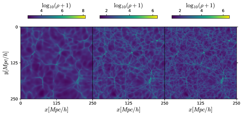
Figure 1: A thin slice of the estimated density field from the simulation boxes at $z=0$ for the three hierarchical levels: from left to right, Smooth 4, Smooth 2, and Smooth 1,  respectively. The effect of the designed filters at $\beta_{s}={4,2,1}$$h^{-1}\mathrm{Mpc}$ is noticeable as we move from left to right.

2 Methods

The cosmic voids are phenomena of the large-scale matter density distribution in the Universe. Since the density is a scale-dependent quantity, the definition and the connected void-finding methodology is a subject of noticeable variation in the field (see eg. Colberg et al. (2008); Libeskind et al. (2018); Cautun et al. (2018)). For the sake of reproducibility and admissibility of comparisons of the results, it is important to clearly define and describe our methodology. This section is devoted to this goal.

2.1 Density field reconstruction

Some studies identified voids directly on the galaxy distribution in order to match observations. However, since our focus lies on describing the inner structure of voids, using the dark-matter (DM) particle distribution rather than the galaxy distribution is better suited for this analysis.

2.1.1 Hierarchical space construction

The analysis presented here is formally based on the Bolshoi simulation with $h=0.7$, $\sigma_{8}=0.82$, and box size, $L=250$$h^{-1}\mathrm{Mpc}$ and a mass resolution of $8.64\times 10^{9}$$M_{\odot}h^{-1}$(the original Bolshoi run has a mass resolution of $1.35\times 10^{8}$$M_{\odot}h^{-1}$(Klypin et al., 2011)). However we use the Bolshoi initial conditions re-sampled on a regular $512^{3}$ particle grid. In order to be able to identify voids at different scales and reconstruct their hierarchical relations we construct a hierarchical space which is a generalization of Gaussian smoothing-based scale-spaces (Aragón-Calvo et al., 2007; Cautun et al., 2015) but explicitly containing hierarchical relations while retaining the anisotropic features of the cosmic web structures.

A hierarchical space is constructed by removing small-scales from the initial conditions of the simulation and then running this smoothed initial conditions as a regular simulation. We use a sharp$-k$ filter as this allows us to cleanly target specific scales to be removed. This filter does not introduce artifacts as it is applied in the linear regime where the Fourier modes are independent (Einasto et al., 2011a; Sheth & van de Weygaert, 2004; van de Weygaert & Sheth, 2004; Einasto et al., 2011b).

Applying such filter one can remove the small-scale details and evolve the filtered density-field to obtain the full non-linear array of substructures above the cut-off scale, $\beta_{s}$.

The resolution in our simulations limits us to three cut-off scales, $\beta_{s}={4,2,1}$$h^{-1}\mathrm{Mpc}$, which we applied to each one of the simulation boxes and the resulting particle distributions are labeled Smooth 4, Smooth 2, and Smooth 1, respectively (see Fig. 1). From the final particle distribution at $z=0$ we estimate the corresponding density fields on a cubic grid of resolution $N_{g}=512^{3}$. Additional steps in order to ensure good quality density fields and to remove small-scale spurious variations can be taken: voxels (cubic pixel) with density values ten times higher than the median of their adjacent voxels are substituted by the mean and the density field is smoothed with a Gaussian filter of $\sigma=2$ voxels. The value of these kernels are the only free parameters in the SpineWeb  framework.

As our motivation lies in studying the internal structure of voids we require a method that excels in reconstructing the density field in the under-dense regions. For this reason we have used the CPU implementation of the Lagrangian Sheet Density Estimator (LSDE) method, originally proposed in Shandarin (2011); Abel et al. (2012). The work of Wojtak et al. (2016) follows the same procedure for estimating their density fields.

To implement the method, the first step involves decomposing the particle grid into tetrahedra in order to compute slices across the 3D Lagrangian tessellation taking advantage that tetrahedra can be used to approximate complex three-dimensional shapes, as they can tessellate space efficiently. This is followed by rendering the tetrahedral decomposition into a data-cube using a triangle-renderer. For each voxel there are eight possible tetrahedral partitions, which are all computed and then the density at each vertex is the resulting average. We chose a cubic grid of 512 cells per size, giving voxels of side-length of 488$h^{-1}$kpc.

2.2 Cosmic web segmentation

The cosmic web is made up of vast, interconnected networks of galaxies and dark matter, which are arranged in a web-like structure that spans the entire observable Universe. This structure has a distinct topology, meaning that it has a specific pattern of connectivity, shape, and arrangement.

In order to understand the cosmic web and its properties, it is important to use methods that take into account its topological nature.

The method we use for identifying the cosmic web components is the SpineWeb algorithm (Aragón-Calvo et al., 2010) which has been specifically designed to capture and analyze the complex, interconnected structure of the cosmic web and takes into account its topology in a comprehensive and accurate way. The SpineWeb  algorithm is based on the watershed segmentation of the density field (Platen et al., 2007).

SpineWeb  begins by identifying all the voxels with the lowest density value among all their 26 neighbours, which will be flagged as the seed for the cosmic voids. Then it runs a topographical distance algorithm finding the maximum gradient paths. After all the voxels are connected to the lowest-density neighbours, the standard flooding algorithm marks the points where two or more watershed regions converge. By identifying all the voxels lying on the watershed boundaries, a morphological label can be attached to discriminate between voxels belonging to a void, a wall, a filament, or a node. This is done by taking advantage of the fact that every voxel in the segmentation is assigned an index numbering the different watershed regions, so by counting the number of neighbouring voids, $N_{v}$, adjacent to a watershed region, we classify each voxel in the boundary as belonging to a void.

This morphological label is assigned by counting the number, $N_{v}$, of voids neighbouring the watershed region. The criteria we use to assign this label are the following: if there are no other voids than the current one (or $N_{v}=1$), it means we are inside of a void; $N_{v}=2$ or having two different adjacent voids means that we are lying in a wall; having $N_{v}=3$ different voids is classified as a filament, and having $N_{v}\geq 4$, is classified as a node. As every voxel is assigned to a watershed region, the case $N_{v}=0$ or no voids found, is not possible.

As a result we have our density field segmented into voxels accordingly labelled as voids, walls, filaments and nodes, which we can merge to obtain the full description of the cosmic web among all three hierarchical scales.

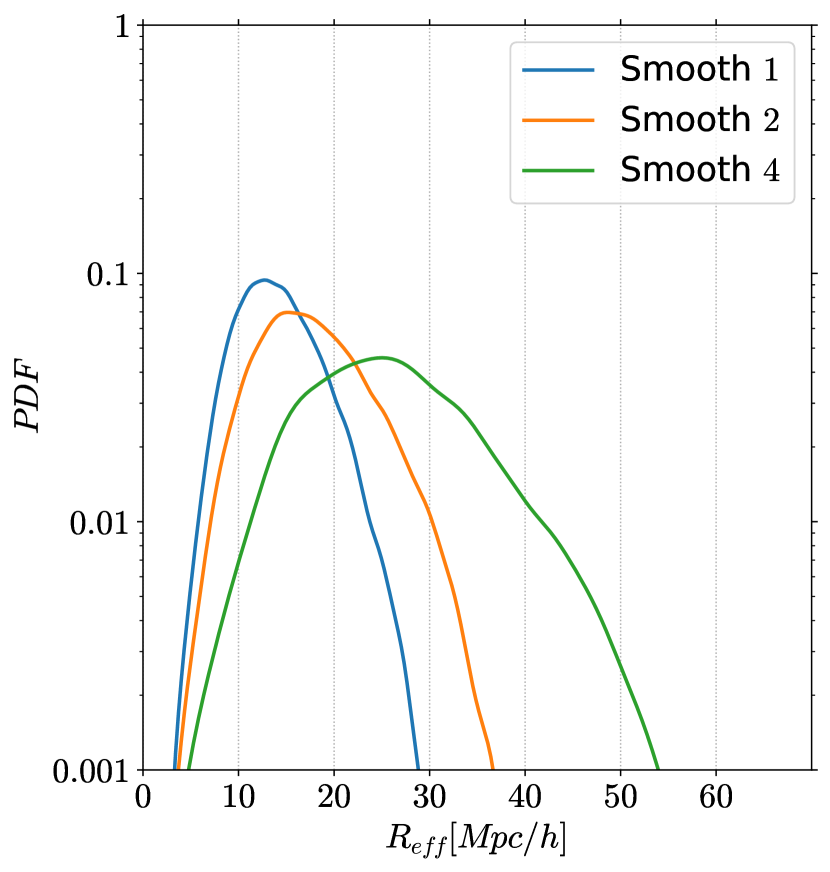
Figure 2: Probability distribution functions for the void sizes in the three hierarchical scales.

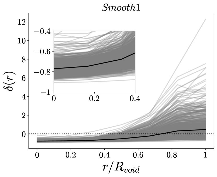
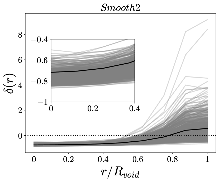
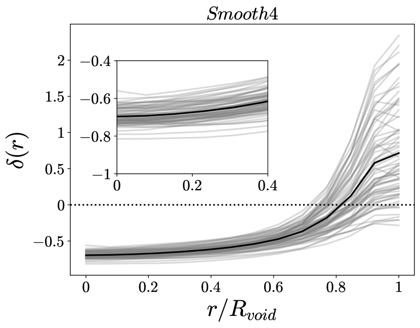
Figure 3: Density profiles for voids across the hierarchy, as function of $R=r/R_{\mathrm{void}}$. The light-gray lines show several individual void profiles while the black line corresponds to the mean of all the profiles. For each hierarchical scale we selected voids with $R_{\mathrm{void}}$ according to the peak of the distributions in 2. The profiles follow the typical bucket-shape form and have the characteristic value of $\delta\sim-0.8$ at the center of the voids, as illustrated in the inset plots.

2.3 Semi-Analytical Galaxy Evolution

Now, in order to characterize the galaxy population tracing each cosmic environment we used the publicly available semi-analytical galaxy evolution software sage (Croton et al., 2016).

sage was designed to work on every $N$-body simulation with appropriately formatted merger trees, which contain full information of the hierarchical growth of the dark matter haloes over cosmic time. Semi-analytical tools then populate each halo with galaxies, using empirical relations and physical models that are carefully fine-tuned to match the observations. Baugh (2006) gives a comprehensive review on semi-analytical tools.

To do so, sage models the baryonic processes that are thought to be important for galaxy formation and evolution, such as gas cooling and heating, gas accretion or ejection, star formation, supernova feedback, black hole growth, and AGN feedback while it keeps track of the gas in satellite galaxies and galaxy mergers as well as the build-up of intra-cluster stars.

Using empirical relations and physical models, sage can predict the properties of galaxies within each halo at different redshifts. The semi-analytical approach models the statistical properties of galaxies very well, however, a detailed discussion of the processes in a single galaxy are beyond the scope of our analysis.

For this part of the analysis we took the halo merger-trees for the full Bolshoi data, which were generated using the friends-of-friends phase space halo finder rockstar (Behroozi et al., 2013a) and consistent-trees (Behroozi et al., 2013b). For the Bolshoi simulation this data is publicly available. The fiducial sage parameters used are described in table 2 of Croton et al. (2016), tuned specifically for the case of the Bolshoi simulation.

The galaxy properties we monitor are: the dimensionless spin parameter, $\lambda$, the masses of host halo, the stellar-to-halo mass relation, and the galaxy metallicities. This allows for an analysis of the galaxies residing in different environments, namely in voids, filaments, walls and clusters, but also, those tracing the filamentary structures found in the inner regions of the larger voids.

3 Results

We present our results related to the hierarchy of the cosmic web in three stages. First we focus on the properties of the reconstructed density fields and the multi-scale nature of the structures imprinted after each filter was applied. Then we discuss their impact on the void properties: void sizes distribution across the hierarchy, and their density profiles. Lastly, we focus on the relationship between the physical properties of haloes and galaxies, and their location in different cosmic web environments.

3.1 Density fields

We illustrate the manner in which the hierarchical structure of the cosmic web is revealed using the filters $\beta_{s}={1,2,4}$$h^{-1}\mathrm{Mpc}$, by presenting a thin slice of the density fields in figure 1. The right-hand panel of the figure shows the density field for the simulated volume applying the least restrictive filter, Smooth 1, where all the large and small-scale details are present in the tenuous filaments and walls surrounding the voids. The middle panel shows the same slice but for the Smooth 2  density field, where only the modes larger than $\beta_{s}=2$$h^{-1}\mathrm{Mpc}$ in the initial power spectrum have evolved and only the structures growing from these modes are preserved. Finally, the left-hand panel shows the bottom of the hierarchy, or Smooth 4, where all the modes below $\beta_{s}=4$$h^{-1}\mathrm{Mpc}$ are absent. In other words, we see that the same large-scale features are present in all 3-levels, be it big voids, massive density knots or elongated filaments. However, by moving from left to right (i.e. from Smooth 1 to Smooth 4) we can observe gradual emergence of smaller “features within features". This simple exercise illustrates the multi-scale nature of the cosmic-web, where all large-scale phenomena such as voids, filaments and even density nodes, contain smaller substructures.

3.2 Void size distribution and density profiles

It is well established that the matter distribution in realistic cosmic voids will never reach a spherically-symmetric arrangement. This is because voids do not live in isolation, but rather are a subject of the tidal-fields induced by the local large-scale structures (Pan et al., 2009; Foster & Nelson, 2009; van de Weygaert, 2014). However, a commonly adopted approach to characterize void sizes, is to use an effective radius of a sphere containing the same volume, $V$, as a given void. This is more convenient than working with 3D volumes themselves, and since majority of voids have quite regular shapes, provides us also with a useful notion of a given void spatial scale. The volume $V$ of a void using the watershed method is computed as the sum of the volumes of all the voxels constituting the void.

We show the distribution of these effective void radii for our three levels of hierarchy in figure 2. We notice how the three curves are very similar and resemble a log-normal distribution. For the top of the hierarchy, the peak of the distribution is around $\sim 12$$h^{-1}\mathrm{Mpc}$, and it moves as we move across the hierarchy, to $\sim 15$$h^{-1}\mathrm{Mpc}$ and $\sim 25$$h^{-1}\mathrm{Mpc}$. We find that the peak scale for each level scales with the smoothing in a simple relation as $R_{\mathrm{peak}}\sim 11\beta_{s}^{0.6}\textrm{$h^{-1}\mathrm{Mpc}$}$.

According to the prevailing theory, voids originate from negative density fluctuations in the primordial density field. Their under-density causes a repulsive force that leads to their expansion. This expansion causes the matter within the voids to move towards their boundaries and results in a void density profile that can be approximated by the shape of a reverse top-hat.

The density profiles for our sample, shown in figure 3, follow the characteristic bucket-shaped form, and the density contrast at the center approaches a value of $\delta\sim-0.8$. Thus, our sample of voids reproduces the well established results of van de Weygaert & Sheth (2004), where $\delta=(\rho-\bar{\rho})/\bar{\rho}$, with $\bar{\rho}$ the background density of the Universe.

In the three panels we notice that, as we get closer to the boundary of each void, the density increases several times the value of $\bar{\rho}$. In the right hand panel, this value increases up to twice the background density, in the middle one, up to 8 times, and in the left one, a dozen times the background value. This is a consequence of two main factors. On the one hand, naturally, the intersection between the corresponding sphere of of radius $R_{\mathrm{eff}}$ and the boundaries of the voids, varies with the void size: for the smaller voids, the sphere with the same volume, $V$, would intersect the void boundaries in couple of points, which are outside of the void and much more dense. On the contrary, the larger voids tend to be more spherical, and in these cases the deviation from an effective sphere description is weaker.

However, a more interesting factor is the effect of the smoothing scale. We have filtered out the smallest voids in Smooth 4 (right panel) and Smooth 2 (middle panel), while having an abundance of small structures at the top of the hierarchy, or Smooth 1 (left panel). In the latter case, the resulting voids are smaller but also the density contrast at their boundaries is larger than in the former cases. In other words, there is a noticeable effect of the web of filaments and nodes delineating the voids, more prominently featured in the unfiltered case (Smooth 1), than in the other two density fields, as we can see in the right-hand ends of the three panels of figure 3.

The result from the cosmic-web segmentation using the morphological label can be seen in the three panels of figure 4. The left-hand panel shows the watershed regions identified as voids, while the middle panel clearly shows the voxels identified as walls. The airtight connection between the boundaries of voids and regions identified as walls is evidenced: as no voxel is left unclassified the walls correspond to a perfectly surrounding structure around voids. Finally, the right-hand panel shows the filaments and nodes surrounding the empty regions.

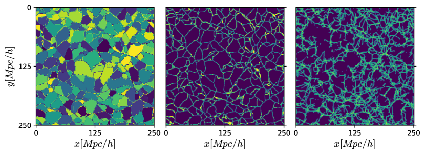
Figure 4: A thin slice of the cosmic web segmentation into voids (left panel), walls (middle panel) and filaments plus nodes (right panel) of the Smooth 4 density field. The tight correspondence of the three environments is evidenced.

3.3 Galaxies tracing the cosmic web

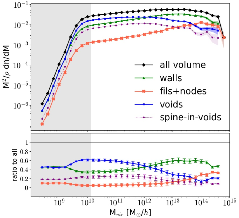
Figure 5: [Top] Differential halo number density as a function of mass for $z=0$. The co-moving number density of haloes less massive than $M$, $n(M,z=0)$, is plotted here as the multiplicity function, $M^{2}\rho^{-1}dn/dM$. The solid black line is the result for the whole volume, the blue squares depict the haloes found in voids, the red crosses are for haloes found in nodes and filaments, the green triangles are for haloes found in walls, and the purple dots for haloes residing in the spine-in-voids. The shaded regions indicate the Poisson errors for each halo mass function. The grey shaded region reflects the mass resolution for haloes of $\geq 10^{2}$ particles. [Bottom] The ratio of each environmental halo mass function with respect to the full sample, the error bars represent the relative Poisson errors for each mass bin.

Table 1: The volume filling fraction of voids, walls, filaments, and nodes, found in each environment for the three levels of the hierarchy, Smooth 1, Smooth 2, and Smooth 4, represented by S1, S2, and S4, respectively. The fractional number of galaxies per environment is indicated in ( ). The fourth column indicates the number of galaxies found in the selected environment across all the hierarchy, this is, $\beta_{123}=\bigcup\beta_{s}$, the union of $\beta_{s}$ with $s=1,2,4$ $h^{-1}\mathrm{Mpc}$. The last column contains the fraction of galaxies found residing in the filamentary structure (nodes, walls, and filaments of Smooth 1) inside of voids at Smooth 4 or spine-in-voids, indicated by $\sigma_{14}$.

	S1	S2	S4	$\beta_{124}$	$\sigma_{14}$
Voids
Vol. frac.	$77.03\%$	$81.71\%$	$86.97\%$	–	–
Frac. gal.	($44.5\%$)	($48.7\%$)	($58.6\%$)	($31.9\%$)	–
Walls
Vol. frac.	$20.31\%$	$16.62\%$	$12.23\%$	–	–
Frac. gal.	($43.4\%$)	($42.0\%$ )	($35.9\%$ )	($19.0\%$)	–
Filaments
Vol. frac.	$2.19\%$	$1.37\%$	$0.61\%$	–	–
Frac. gal.	($10.0\%$ )	($7.7\%$)	($4.5\%$)	($0.8\%$)	–
Nodes
Vol. frac.	$0.46\%$	$0.31\%$	$0.21\%$	–	–
Frac. gal.	($2.01\%$)	($1.52\%$)	($0.89\%$)	($0.02\%$)	–
spine-in-voids
Frac. gal.	-	-	-	-	(22.8 $\%$)

After running sage with the parameters according to Croton et al. (2016) for Bolshoi, we identified a total of 7 909 721, or $\sim(199)^{3}$, galaxies at redshift $z=0$, fulfilling the condition of $M_{*}>0$. From those, approximately a third of the full sample (32$\%$), was found in voids across the three hierarchy levels, $19\%$, were residing in walls, $0.8\%$ in filaments and $0.02\%$ in nodes.

This corresponds to the fifth column of table 1. We have defined the full hierarchy, $\beta_{124}=\bigcup\beta_{s}$, with the condition that a given galaxy belongs to the same environment in all the three scales simultaneously. Roughly half of the sample matches this criterion.

Now, to look at how these fractions distribute across the hierarchy, we also include the fractional number of galaxies per environment in Smooth 1, Smooth 2,  and Smooth 4. See columns 2, 3, and 4 of table 1, respectively. In this case the fractions add up to 100$\%$ in each level of the hierarchy. From these numbers we notice the impact that the scale of description has in the classification of the membership of galaxies. For instance, at the top of the hierarchy we have almost the same percentage of galaxies located voids ($44.5\%$) as we do find in walls ($43.4\%$). With a yet smaller fraction of galaxies tracing filaments ($10\%$), and a minuscule population found in nodes, the densest environments ($2\%$). However, as we move through the hierarchy, from Smooth 1 to Smooth 2 and Smooth 4, we can see how those fractions change. The fraction of galaxies found in voids increases (from $45\%$ to $49\%$ and finally, $59\%$), and, consequently, the fraction of galaxies in denser environments diminishes.

This is a direct consequence of the change in the volume filling fractions of each environment. The volume filled by voids changes from $77\%$ to $87\%$, as we go from Smooth 1 to Smooth 4, and consequently, the volume filled by walls, filaments and nodes, decreases.

Now, in order to identify the population of galaxies tracing the inner structures of voids, we select voids in the Smooth 4 of the hierarchy and for each one, we map the corresponding filamentary structure (walls+filaments+nodes) identified in Smooth 1. We shall consider such defined population as tracing a distinct new environment, which we dub spine-in-voids, and which comprises $23\%$ of the full galaxy sample (see last column of table 1).

Having defined and described our galaxy samples split among our cosmic web environments, we now take a look on how different physical properties of galaxies vary across different population. In what follows we consider (A) the halo-mass-function (HMF), (B) their spin, $\lambda$, (C) the stellar-to-halo mass (SHM) relation, and (D) their metallicities, in the context of the galaxies placement in the cosmic web.

A. Environmental HMF

The function $n(M,z)$ gives the comoving number density of haloes with a virial mass below $M_{\mathrm{vir}}$, denoted by $M$ to simplify the notation. In figure 5, we show it as the halo multiplicity function $M^{2}\rho^{-1}\mathrm{d}n/\mathrm{d}M$, with $\rho$, the mean density of the Universe, and also for each cosmic web type.

The full sample is represented in black diamonds, while the galaxies split by cosmic environment are represented as follows: red crosses for galaxies found in nodes and filaments, green triangles for walls, and blue squares for galaxies residing in voids. The purple dots represent the galaxies found in the spine-in-voids environment.

Our halo mass functions cover 6 orders of magnitude in mass, from $10^{9}-10^{15}[M_{\odot}h^{-1}]$. To ensure robustness in our analysis, we have set a minimum particle threshold for halo identification. We add a shaded region to indicate a halo mass convergence threshold, set at a minimum of 100 particles per group, which we believe is a conservative choice given that previous studies in the literature (Behroozi et al., 2013a; Croton et al., 2016) report a threshold of 20 and 50 particles per halo, respectively. However, the 100 particle threshold was found to be a reasonable value for the convergence of a simulated FoF groups HMF in Warren et al. (2006). Therefore, we do not consider HMF, and so also the halo and galaxy populations, as converged below masses of $1.35\times 10^{10}$$M_{\odot}h^{-1}$.

The first thing we notice from the environmental HMF split is that the galaxies at the low mass end are found mostly residing in voids; this is, for masses up to $10^{12}$$M_{\odot}h^{-1}$, at which point, the number of galaxies residing on walls start to dominate the high mass end.

Another feature to note is the low number counts of galaxies residing in the densest environments such as filaments and nodes. We attribute this results as due to a specific systematic induced by the classification scheme. As detailed in subsection 2.2, the voxels residing in the border between voids were marked with a morphological label, which, depending on the number of different neighbouring voids, were classified as a walls ($\mathcal{N}_{v}=2$), filaments ($\mathcal{N}_{v}=3$) or nodes ($\mathcal{N}_{v}\geq 3$). In each case, the environments are 1-voxel thick, resulting in vanishingly small volume-filling fractions leading to artificially lower number of galaxies identified in such environments. This is clearly demonstrated by the volume-filling fractions quoted in table 1, where we can see that the volume occupied by filaments fluctuates between 2.19$\%$ and 0.61$\%$, while the volume occupied by nodes is practically negligible. For this reason we plot the halo mass function for filaments and nodes jointly.

However, a difference between environments can be noticed through the increasing steepness of the HMF for the densest environments (filaments+nodes) at the high mass end, more pronounced than the one for walls, and in opposite direction than the HMFs for haloes residing in voids and in the spine-in-voids. Respect to the latter, their HMF follows the same behaviour as the haloes found in voids but with a lower number count. As indicated in the last column of table 1, this sample comprises 23$\%$ of the full sample.

The lower-panel of figure 5 illustrates the relative fraction of haloes found in each one of the environments with respect to the full volume. A striking feature is the threshold value for the mass at around $10^{12}$$M_{\odot}h^{-1}$, at which the fraction of haloes residing in walls starts to dominate at the high-mass end. For haloes with masses below this value, the dominant population is residing in voids. The fraction of haloes found in the densest environments is heavily suppressed during the full mass range, except by the last mass bin, at $M_{\mathrm{vir}}\sim 10^{15}$$M_{\odot}h^{-1}$, where the full sample resides in nodes. For a cleaner visualisation we omit the last bin in the ratios depicted in the bottom panel of figure 5.

B. Spin

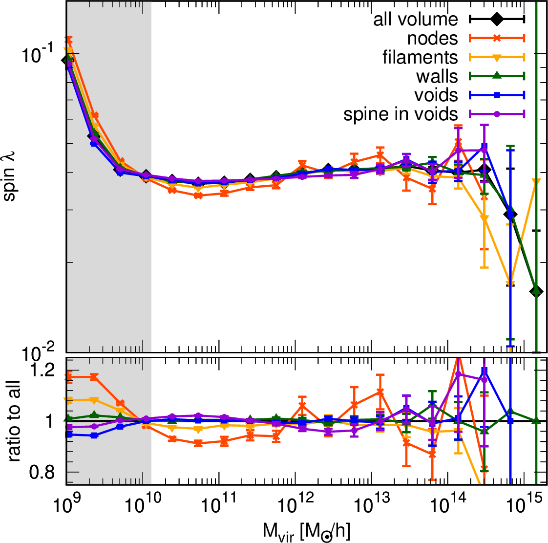
Figure 6: [Top] Value of the spin parameter, $\lambda$, for the galaxies located in different cosmic environments. In black diamonds we indicate the full sample, red crosses, haloes found in nodes, green triangles are for walls, inverted yellow triangles are filaments, blue squares represent voids and the purple dots, the haloes found in the spine-in-voids. [Bottom] Ratio of each environment with respect to the full sample. The shaded gray areas represent the mass resolution limitation of 100 particles per halo. The errors indicate a bootstrap on the medians per mass bin.

Another relevant property for dark matter haloes, besides their mass is their internal structure. One of the physical properties describing the internal structure of dark matter haloes is the spin parameter, which provides a measure of the net internal rotation of the dark matter halo and is typically provided in terms of their angular momentum. sage follows the definition from Bullock et al. (2001) for the spin parameter of dark matter halos, $\lambda=\lvert J\rvert/\sqrt{2}R_{\mathrm{vir}}V_{\mathrm{vir}}$, where $|J|=S_{x}^{2}+S_{y}^{2}+S_{z}^{2}$ is the halo total angular momentum, and $R_{\mathrm{vir}}$ and $V_{\mathrm{vir}}$, the virial radius and virial velocity of the halo, respectively.

In figure 6 we show the spin parameter of the fraction of haloes found in each of the LSS environments in a given mass bin. The bottom panel shows the relative difference between each environment and the total volume. In this case the galaxies split by cosmic environment are: red crosses for the node-halo sample, green triangles for walls, yellow inverted triangles for filaments, blue squares for void galaxies, and purple dots haloes found in the spine-in-voids environment.

For each halo mass bin, we estimate the uncertainties through a bootstrap of the median, using 100 bootstrap samples. We found that the overall shape of the spin as a function of $M_{\mathrm{vir}}$ is relatively flat around the value $\lambda=0.04$. However, when we analyzed the relative ratio of spin properties for each cosmic web halo population with respect to the all-volume sample, we observed some environmental effects, for haloes with masses between $10^{10}-10^{12}$$M_{\odot}h^{-1}$, and peaking around $10.4-10.6\times 10^{10}$$M_{\odot}h^{-1}$, the range for which we have the strongest environmental effects.

In this mass range there is a clear trend showing that haloes found in the densest environments get a suppression of their spin, while the haloes in the less dense environments such as voids or spine-in-voids  have an enhancement in their angular momentum. In particular, we found that the spin of haloes in nodes, which are the densest regions of the cosmic web, exhibits a suppression of approximately 10$\%$ compared to the full sample. Similarly, we observed a suppression of spin for haloes in filaments, although of smaller proportions. The haloes in walls seem to be unaffected with respect to the overall sample, but those found in the less dense environments, do show an increase of their spin. This effect was recently observed around Milky Way analogues located in walls (Aragon-Calvo et al., 2023). Interestingly, this enhancement is stronger for the haloes in the spine-in-voids environment than for the haloes in voids.

For haloes with $M_{\mathrm{vir}}>10^{12}$$M_{\odot}h^{-1}$, we did not observe any significant patterns in the spin properties with respect to the cosmic web environment.

C. Stellar-to-halo mass relation

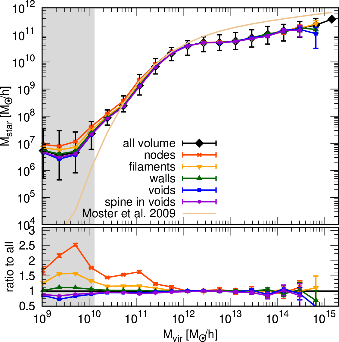
Figure 7: [Top] Stellar-to-halo mass relation, $M_{\star}$ - $M_{\mathrm{vir}}$ as function of the environment. Black diamonds indicate the full sample, red crosses, haloes found in nodes, green triangles are for walls, inverted yellow triangles are filaments, blue squares represent voids and the purple dots, the haloes found in the spine-in-voids. The solid golden line reflects the prediction of Moster et al. (2010). [Bottom] Ratio of each environmental SHM function with respect to the full sample. The shaded gray areas represent the mass resolution limitation of 100 particles per halo. The errors indicate a bootstrap on the medians per mass bin.

The link between galaxy properties and their host DM haloes can be understood via the stellar-to-halo mass (SHM) relation. To demonstrate the effect of the environment on the SHM function, we plot the stellar mass, $M_{*}$, as function of the mass of the host halo, $M_{\mathrm{vir}}$, in figure 7, for the full sample, and also for each cosmic environment with the same legends as explained above.

We compare our results with the parametric fit proposed by Moster et al. (2010), whose estimation for the stellar mass agrees with the trend of our sample in the halo mass range $10.3\times 10^{10}-10.1\times 10^{12}$ [$M_{\odot}h^{-1}$].

To emphasize the effect of the environment on the SHM relation, in the bottom panel of 7, we plot the ratio of each individual cosmic environment to the total galaxies sample.

A very interesting feature arises from analyzing these ratios. A clear dependence on the environment is present for haloes below the mass threshold of $M_{\mathrm{vir}}<10^{12}$$M_{\odot}h^{-1}$. The environmental dependence on the SHMR is the most prominent for the node-galaxy population, in which case we see an enhancement above $50\%$ with respect to the stellar mass of the full sample. The galaxies in filaments, we can also observe an increase in their stellar masses, close to $15\%$. The maximum departure is found for galaxies in haloes of masses around $10^{11}$$M_{\odot}h^{-1}$. As for the galaxies found in walls, we find no significant departure from the overall SHMR, and a small decrease of stellar masses is seen for the galaxy samples residing in voids and in the spine-in-voids environment.

For galaxies hosted in haloes of masses above the threshold, $M_{\mathrm{vir}}>10^{12}$$M_{\odot}h^{-1}$, the environmental split seems to be a subdominant effect on their stellar content.

D. Metallicity

Another property of galaxies helping bridge our understanding between galaxy formation and evolution with their cosmic web location, is the metal contents of galaxies. The metal content or metallicity, expressed as $12+\log_{10}(O/H)$, provides a measure of the efficiency of stars in forming metals. Figure 8 shows the metal fraction as function of stellar mass, split by environment.

The main trend of all of our samples corresponds to an increasing function of metal content for higher stellar masses, which lies in agreement with the observational result reported by Tremonti et al. (2004), for galaxies with stellar masses in the range of $1.1\times 10^{9}-1.2\times 10^{10}$$M_{\odot}h^{-1}$.

Beyond this overall trend, the environmental dependence is noticeable.

The densest environments, corresponding to nodes and filaments of the cosmic web, exhibit a pronounced enhancement of their metallicities compared to the full sample. This enhancement reaches a maximum of  25$\%$, for stellar masses of $10^{8}-10^{9}$$M_{\odot}h^{-1}$, declining and vanishing for $M_{*}\sim 10.2^{10}$$M_{\odot}h^{-1}$. The filaments show a very similar yet less prominent effect, while the metallicities of galaxies residing in walls show no difference with respect to the overall sample. As for the low density environments, such as voids and spine-in-voids, we see a reduction of their metallicities of almost 10$\%$, for masses in the same range, $M_{*}<10^{10}$$M_{\odot}h^{-1}$. In this case, we see that the population of galaxies residing in the spine-in-voids environment suffer from the same reduction of their metal fraction in comparison with the full sample, as do our void-galaxies sample. Galaxies with higher stellar masses than $10^{10}$$M_{\odot}h^{-1}$, do not have a discernible trend in their metallicities with respect of the cosmic web environment where they reside.

As we could see in our previous result, the stellar mass of galaxies shows a discernible dependence on the cosmic web environment, in particular, a trend of increased stellar mass for the galaxies residing in the denser environments, and a reduced gas content for galaxies in voids. It is well known that the relationship between stellar mass and metallicity works as a diagnostic of the physical processes that govern galaxy formation and evolution. In sage, this connection is modelled assuming a yield, $Y$, or fraction of the stellar mass that is converted into metals during the process of stellar evolution. Hence, the environmental dependence of the SHMR, gets imprinted in the metallicities-$M_{*}$ plane with similarly distinctive signatures.

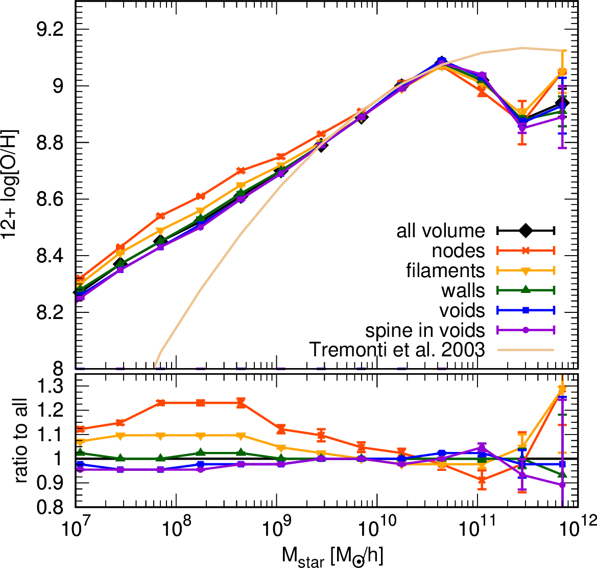
Figure 8: [Top] Metallicity as function of stellar mass, $M_{*}$. We report the ratio of Oxygen to Hydrogen in units of $12+\log(O/H)$ and compare our results with the formula presented in Tremonti et al. (2004) (golden line). In black diamonds we indicate the metallicities of galaxies for full sample, red crosses are for haloes found in nodes, green triangles for walls, inverted yellow triangles are filaments, blue squares represent voids and the purple dots are for the haloes found in the spine-in-voids. [Bottom] The relative difference per each environment with respect to the full sample.

4 Discussion

In this paper we have presented an in-depth analysis of the connection between galaxy properties and the internal structure of voids using cosmological simulations. While some works have extensively looked at both factors separately, we aimed to study the interplay between both.

The ability to select and describe the inner structure of voids relied on the implementation of appropriate filters selecting specific scales ($\beta_{s}=1,2,4$$h^{-1}\mathrm{Mpc}$) in the gravity-only simulations and constructing a hierarchy of voids, walls, filaments and nodes, similarly to the work of Aragon-Calvo & Szalay (2012).

However, by further populating the DM haloes with galaxies, using the numerical implementation of the sage method, we were able to pose the question of what population of galaxies traces the internal filamentary structure of voids, or spine-in-voids, as we named such environment, in terms of their halo mass function, spin, stellar mass, and metallicity.

To characterize such hierarchical structure of voids, we presented the void size functions and density profiles, as function of the smoothing scale, $\beta_{s}$. Our results agree with previous results regarding the density profile of voids identified using watershed techniques (see for instance van de Weygaert (2014); Cautun et al. (2018)), but they also show the effect of the smoothing scale, $\beta_{s}=1,2,4$$h^{-1}\mathrm{Mpc}$.

With respect to the void size functions, we found that the peak of the PDFs scales with the smoothing scale through a simple relationship as: $R_{\mathrm{peak}}\sim 11\beta_{s}^{0.6}$$h^{-1}\mathrm{Mpc}$.

We found a strong environmental dependence on our HMFs (see figure 5). A threshold of $M_{\mathrm{th}}\sim 10^{12}M_{\odot}h^{-1}$marks the turnover between haloes in voids and haloes in walls dominating the number counts, and it is present prominently in the HMFs. We adjudicate the low number counts of haloes in filaments and nodes to the morphological labeling in our cosmic web segmentation, in particular to artificially thin (one-voxel thick) environments other than voids. Conversely, our number of void-galaxies is quite large (45-59$\%$), which we attribute to the watershed technique being a volume filling algorithm, which by construction returns too thin filaments, and potentially leads to mislabelling galaxies at the edge of the voids as void-galaxies instead of wall, filaments or node-galaxies.

The newly defined environment, spine-in-voids, shows the same behaviour as the void-galaxy sample, but with suppressed number counts, signaling that the dominating effect is the one of being found in a low-density environment, just as void-galaxies are.

Interestingly enough, the other quantity related to describe the properties of dark matter haloes, i.e. the spin parameter $\lambda$, shows environmental effects for a mass below the same threshold $M_{\mathrm{th}}\sim 10^{12}M_{\odot}h^{-1}$. In this case, however, we find that the haloes located in the densest regions of the cosmic web have a smaller spin parameter compared to those in voids. This suppression is stronger for haloes in nodes and to a lesser extend for those in filaments, suggesting that the tidal forces exerted by the surrounding large-scale structures play a role in shaping the spin of haloes. The haloes found in the under-dense regions, on the other hand, show a slight enhancement in their spin parameter with respect to the trend of the full sample. Our results lie in agreement with the work of Peper & Roukema (2021), where similar void-finding and halo identification techniques were used. We found the overall shape of the $\lambda(M_{\mathrm{vir}})$ function to be relatively flat around the value $\lambda=0.04$, which is a slightly higher value than the one reported as the peaks of the distributions reported by Avila-Reese et al. (2005). Nevertheless we agree in reporting higher values of $\lambda$ for void galaxies, and smaller for galaxies in high density environments.

However, when holding our results against those reported by Hellwing et al. (2021), the comparison is not as direct, as we have probed different mass ranges in our halo catalogues. While they report a similar decrease in the spin parameter for their node-haloes, in the mass range of $M_{\mathrm{vir}}\sim 10.6\times 10^{7}-10^{10}$$M_{\odot}h^{-1}$, and also a minimal enhancement for the spin of their void-haloes, in the same mass range, they have a substantial further decrease of the spin of the void sample. This reduction of spin is of almost 35$\%$, as they quote, and is present for haloes of masses around $10^{11}$$M_{\odot}h^{-1}$in $M_{\mathrm{vir}}$. Care should be taken when attempting a direct comparison, though, as we have different mass ranges of our halo samples. For instance, we do have void-haloes at all mass ranges, whereas, the authors of this work only have them for masses below $10.4\times 10^{11}$$M_{\odot}h^{-1}$. As our cosmic web segmentation methods are different (the authors have implemented NEXUS which is a Hessian-based method, that classifies the cosmic web based on the tidal tensor signatures), and also our halo identification schemes differ, discrepancies are to be expected. However, the main trend hinting to a suppression of $\lambda$ for haloes residing in the densest environments is present in both our works, as well as the detection of a mass threshold at which the various cosmic web populations deviate from the mean trend describing the overall halo population. In our work, this mass threshold is of the order $M_{\mathrm{th}}\sim 10^{12}$$M_{\odot}h^{-1}$, over two orders of magnitude higher than the mass-scale reported by Hellwing et al. (2021).

Understanding the interplay between the cosmic web and the properties of galaxies is crucial in modern cosmology. While dark matter haloes provide a convenient framework to study the formation and evolution of galaxies, they are not observable, and therefore it is important to go beyond their properties and analyze the stellar content and metallicities of galaxies in terms of their placement on the cosmic web.

In this case, our major finding shows that our stellar-to-halo mass functions reflect a strong environmental dependence for masses below $M_{\mathrm{th}}\sim 10^{12}M_{\odot}h^{-1}$, the same mass threshold as the one reported for halo properties. In particular, we see a significant increase of stellar masses for haloes in nodes and filaments, in the range $M_{\mathrm{vir}}<M_{\mathrm{th}}$. For the galaxies identified in the under-dense regions, we have a decreased stellar mass ratio in the same mass range, in agreement with previous works (see for instance Hoyle et al. (2005); Croton et al. (2005); Moorman et al. (2015)).

As for the metallicities or the abundance of elements heavier than helium, usually expressed as the ratio of the mass of these elements to the mass of hydrogen, the major trends follow the same pattern: a strong environmental dependence showing that galaxies in high density environments (nodes, filaments, and walls) have sharp increases in their metal abundances, with respect to the full sample, while the galaxies populating the low-density environments (voids and spine-in-voids) presented a decreased metallicity value as function of $M_{*}$. In this case we observe that the environmental effects are present for masses below $M_{*}\sim 10.1\times 10^{10}$$M_{\odot}h^{-1}$. Interestingly, we find that the population spine-in-voids  shows a slightly stronger suppression of metallicities, when compared to the full sample.

The previous results are consistent with the expectation that galaxy mergers and interactions are more frequent in denser environments, leading to a higher star formation rate and, thus, greater rate of metal production. This expectation aligns with the idea of nodes and filaments having a higher probability of hosting massive star-forming galaxies and clusters, which are known to be efficient in producing metals through their stellar winds and supernova explosions. Our findings provide further evidence that the cosmic web plays a critical role in the formation and evolution of galaxies, with the denser regions being more conducive to metal formation.

Furthermore, even if metallicity is not a perfect indicator of a galaxy’s age (for instance, a galaxy can undergo episodes of enhanced star formation that can boost their metallicity without significantly increasing its age, but also periods of gas accretion which can dilute their metallicities without affecting the age), it is well known that it can be used as a proxy for a galaxy’s age as it is easier to determine the abundance of heavy elements observationally, as to directly measure the age. From this it follows that our results support the picture of void galaxies being younger (bluer), and galaxies in nodes or filaments, older (redder). Respect to the spine-in-voids-galaxy sample, we conclude that their properties follow those of the void-galaxies in general. In the case of their metallicities, we found a slight decrease in their metal fraction with respect to the full sample. We interpret this further suppression as an effect of the more frequent gas accretion periods, which can be fed via the filaments connecting such galaxies with the boundaries of the voids, and diluting their metallicities.

5 Conclusions

We analyzed the link between a galaxy’s location in the cosmic web and its physical properties such as their morphology (spin), size (mass), stellar mass ($M_{*}$), and metallicity. Our methodology allowed us to select the filamentary structure in the interior of cosmic voids and to characterize the sample of galaxies tracing such cosmic web environment, which we named spine-in-voids.

The cosmic web segmentation was done by implementing the watershed algorithm, or SpineWeb on a set of gravity-only simulations which were a lower resolution of the Bolshoi cosmological simulation. The galaxies were added by implementing the semi-analytical galaxy evolution code, sage, using the available halo-trees for the full-resolution Bolshoi simulation. Under this scheme, the merger trees are extracted from a DM-only $N$-body simulation and gas processes are treated with semi-analytic recipes.

The specific segmentation, even if parameter-free, introduced a systematic effect in artificially low number counts for the densest environments, particularly visible in our HMFs. Nevertheless, our results show that the stellar mass and metallicity of galaxies are significantly influenced by their location within the cosmic web, as well as the halo properties such as their mass functions and spin.

An interesting result we found throughout our analysis was a threshold mass: $M_{\mathrm{th}}\sim 10^{12}M_{\odot}h^{-1}$, fixing the mass range for which we see environmental dependence in the galaxies properties. This value is in agreement with the expectation of haloes with masses larger than $10^{12}$$M_{\odot}h^{-1}$, to be predominantly in dense environments. In particular, for the halo mass functions, this $M_{\mathrm{th}}$ signals the turnover between void-haloes and wall-haloes dominating the number counts in the HMFs. For the spin parameter, $\lambda$, we see an environmental dependence for haloes below this $M_{\mathrm{th}}$. Particularly, our results show that haloes in denser environments get a suppression of their spin with respect to the full sample, whereas haloes in under-dense regions suffer a slight increase in their angular momentum. We interpret this result as the effect of the tidal forces exerted by the surrounding large-scale structures, playing a role in shaping the spin of haloes. This same threshold gets imprinted in the stellar content of the galaxies.

An interesting follow up would be to apply the SpineWeb framework to address the question of how the properties of galaxies change as function of their distance with respect to different points in the cosmic web, for instance, the center of the void or with respect to the walls or the nearest filament. For example, the authors of Peper & Roukema (2021) have searched into the different definitions of void center to quantify the effect on the halo properties. Others, for instance Tavasoli (2021), have quantified the effect in the geometrical position of void galaxies, looking at density profiles of stacked voids. Also, the authors of Donnan et al. (2022) report finding a trend between the metallicity of galaxies as function of their distances to filaments detected in simulations. As all of the aforementioned works use different methods and data, and we know that there are a diversity of results regarding the connection between galaxy formation an evolution versus their cosmic web placement, we think that this as future analysis would be a worthwhile path of research.

To summarize, we have shown that the properties of galaxies tracing the internal structure of voids can be described to have smaller stellar masses and to be located in haloes with smaller $M_{\mathrm{vir}}$, to have an enhanced spin, and a lower metallicity. Our findings provide further evidence that the environmental effect is present for certain threshold in mass. Specifically, we found that the cosmic web plays a critical role for galaxies with $M_{\mathrm{vir}}\sim 10^{11}$$M_{\odot}h^{-1}$and $M_{*}\sim 10^{8}$$M_{\odot}h^{-1}$. These results altogether point to the need of testing our framework on higher resolution simulations to explore the effect of cosmic web environment on satellite galaxies.

Data Availability

The halo trees used in this work are publicly available at this URL, and the numerical implementation of the density estimator can be found in this repository. The version of the code sage can be downloaded from sage. The SpineWeb code and data underlying this article will be shared upon reasonable request to the corresponding author.

References

- Abazajian et al. (2009) Abazajian K. N., et al., 2009, ApJS, 182, 543
- Abel et al. (2012) Abel T., Hahn O., Kaehler R., 2012, MNRAS, 427, 61
- Alpaslan et al. (2014) Alpaslan M., et al., 2014, MNRAS, 440, L106
- Aragon-Calvo (2023) Aragon-Calvo M. A., 2023, MNRAS, 522, L46
- Aragon-Calvo & Szalay (2012) Aragon-Calvo M. A., Szalay A. S., 2012, Monthly Notices of the Royal Astronomical Society, 428, 3409
- Aragón-Calvo et al. (2007) Aragón-Calvo M. A., Jones B. J. T., van de Weygaert R., van der Hulst J. M., 2007, A&A, 474, 315
- Aragón-Calvo et al. (2010) Aragón-Calvo M. A., Platen E., van de Weygaert R., Szalay A. S., 2010, The Astrophysical Journal, 723, 364
- Aragon-Calvo et al. (2023) Aragon-Calvo M. A., Silk J., Neyrinck M., 2023, MNRAS, 520, L28
- Aubert et al. (2022) Aubert M., et al., 2022, MNRAS, 513, 186
- Avila-Reese et al. (2005) Avila-Reese V., Colín P., Gottlöber S., Firmani C., Maulbetsch C., 2005, ApJ, 634, 51
- Baugh (2006) Baugh C. M., 2006, Reports on Progress in Physics, 69, 3101
- Behroozi et al. (2013a) Behroozi P. S., Wechsler R. H., Wu H.-Y., 2013a, ApJ, 762, 109
- Behroozi et al. (2013b) Behroozi P. S., Wechsler R. H., Wu H.-Y., Busha M. T., Klypin A. A., Primack J. R., 2013b, ApJ, 763, 18
- Beygu et al. (2016) Beygu B., Kreckel K., van der Hulst J. M., Jarrett T. H., Peletier R., van de Weygaert R., van Gorkom J. H., Aragon-Calvo M. A., 2016, MNRAS, 458, 394
- Borzyszkowski et al. (2017) Borzyszkowski M., Porciani C., Romano-Díaz E., Garaldi E., 2017, MNRAS, 469, 594
- Bullock et al. (2001) Bullock J. S., Dekel A., Kolatt T. S., Kravtsov A. V., Klypin A. A., Porciani C., Primack J. R., 2001, ApJ, 555, 240
- Cai et al. (2016) Cai Y.-C., Taylor A., Peacock J. A., Padilla N., 2016, MNRAS, 462, 2465
- Cautun et al. (2015) Cautun M., van de Weygaert R., Jones B. J. T., Frenk C. S., Hellwing W. A., 2015, in Thirteenth Marcel Grossmann Meeting: On Recent Developments in Theoretical and Experimental General Relativity, Astrophysics and Relativistic Field Theories. pp 2115–2117 (arXiv:1211.3574), doi:10.1142/9789814623995_0371
- Cautun et al. (2018) Cautun M., Paillas E., Cai Y.-C., Bose S., Armijo J., Li B., Padilla N., 2018, MNRAS, 476, 3195
- Chincarini & Rood (1975) Chincarini G., Rood H. J., 1975, Nature, 257, 294
- Colberg et al. (2008) Colberg J. M., et al., 2008, MNRAS, 387, 933
- Colless et al. (2003) Colless M., et al., 2003, arXiv e-prints, pp astro–ph/0306581
- Contarini et al. (2019) Contarini S., Ronconi T., Marulli F., Moscardini L., Veropalumbo A., Baldi M., 2019, MNRAS, 488, 3526
- Correa et al. (2021) Correa C. M., Paz D. J., Sánchez A. G., Ruiz A. N., Padilla N. D., Angulo R. E., 2021, MNRAS, 500, 911
- Croton et al. (2005) Croton D. J., et al., 2005, MNRAS, 356, 1155
- Croton et al. (2016) Croton D. J., et al., 2016, ApJS, 222, 22
- Domínguez-Gómez et al. (2022) Domínguez-Gómez J., et al., 2022, A&A, 658, A124
- Donnan et al. (2022) Donnan C. T., Tojeiro R., Kraljic K., 2022, Nature Astronomy, 6, 599
- Doroshkevich et al. (1978) Doroshkevich A. G., Shandarin S. F., Saar E., 1978, MNRAS, 184, 643
- Einasto et al. (2011a) Einasto J., et al., 2011a, A&A, 531, A75
- Einasto et al. (2011b) Einasto J., et al., 2011b, A&A, 534, A128
- Fang et al. (2019) Fang Y., et al., 2019, MNRAS, 490, 3573
- Florez et al. (2021) Florez J., et al., 2021, ApJ, 906, 97
- Foster & Nelson (2009) Foster C., Nelson L. A., 2009, ApJ, 699, 1252
- Gottlöber et al. (2003) Gottlöber S., Łokas E. L., Klypin A., Hoffman Y., 2003, MNRAS, 344, 715
- Granett et al. (2008) Granett B. R., Neyrinck M. C., Szapudi I., 2008, ApJ, 683, L99
- Gregory & Thompson (1978) Gregory S. A., Thompson L. A., 1978, Nature, 274, 450
- Hellwing et al. (2021) Hellwing W. A., Cautun M., van de Weygaert R., Jones B. T., 2021, Phys. Rev. D, 103, 063517
- Hoyle et al. (2005) Hoyle F., Rojas R. R., Vogeley M. S., Brinkmann J., 2005, ApJ, 620, 618
- Jennings et al. (2013) Jennings E., Li Y., Hu W., 2013, MNRAS, 434, 2167
- Kirshner et al. (1981) Kirshner R. P., Oemler A. J., Schechter P. L., Shectman S. A., 1981, ApJ, 248, L57
- Kirshner et al. (1987) Kirshner R. P., Oemler Augustus J., Schechter P. L., Shectman S. A., 1987, ApJ, 314, 493
- Klypin et al. (2011) Klypin A. A., Trujillo-Gomez S., Primack J., 2011, ApJ, 740, 102
- Krause et al. (2013) Krause E., Chang T.-C., Doré O., Umetsu K., 2013, ApJ, 762, L20
- Kreckel et al. (2011) Kreckel K., et al., 2011, AJ, 141, 4
- Libeskind et al. (2018) Libeskind N. I., et al., 2018, MNRAS, 473, 1195
- Moorman et al. (2015) Moorman C. M., Vogeley M. S., Hoyle F., Pan D. C., Haynes M. P., Giovanelli R., 2015, ApJ, 810, 108
- Moster et al. (2010) Moster B. P., Somerville R. S., Maulbetsch C., van den Bosch F. C., Macciò A. V., Naab T., Oser L., 2010, ApJ, 710, 903
- Nadathur & Crittenden (2016) Nadathur S., Crittenden R., 2016, ApJ, 830, L19
- Nadathur & Percival (2019) Nadathur S., Percival W. J., 2019, MNRAS, 483, 3472
- Nadathur et al. (2019a) Nadathur S., Carter P. M., Percival W. J., Winther H. A., Bautista J. E., 2019a, Phys. Rev. D, 100, 023504
- Nadathur et al. (2019b) Nadathur S., Carter P., Percival W. J., 2019b, MNRAS, 482, 2459
- Nadathur et al. (2020) Nadathur S., et al., 2020, MNRAS, 499, 4140
- Paillas et al. (2019) Paillas E., Cautun M., Li B., Cai Y.-C., Padilla N., Armijo J., Bose S., 2019, MNRAS, 484, 1149
- Pan et al. (2009) Pan D., Hoyle F., Vogeley M. S., 2009, in American Astronomical Society Meeting Abstracts #213. p. 425.07
- Pan et al. (2012) Pan D. C., Vogeley M. S., Hoyle F., Choi Y.-Y., Park C., 2012, MNRAS, 421, 926
- Patiri et al. (2006) Patiri S. G., Prada F., Holtzman J., Klypin A., Betancort-Rijo J., 2006, MNRAS, 372, 1710
- Peper & Roukema (2021) Peper M., Roukema B. F., 2021, MNRAS, 505, 1223
- Pisani et al. (2015) Pisani A., Sutter P. M., Hamaus N., Alizadeh E., Biswas R., Wandelt B. D., Hirata C. M., 2015, Phys. Rev. D, 92, 083531
- Platen et al. (2007) Platen E., van de Weygaert R., Jones B. J. T., 2007, MNRAS, 380, 551
- Pranav et al. (2017) Pranav P., Edelsbrunner H., van de Weygaert R., Vegter G., Kerber M., Jones B. J. T., Wintraecken M., 2017, MNRAS, 465, 4281
- Shandarin (2011) Shandarin S. F., 2011, J. Cosmology Astropart. Phys., 2011, 015
- Sheth & van de Weygaert (2004) Sheth R. K., van de Weygaert R., 2004, Monthly Notices of the Royal Astronomical Society, 350, 517
- Sutter et al. (2012) Sutter P. M., Lavaux G., Wandelt B. D., Weinberg D. H., 2012, ApJ, 761, 187
- Sutter et al. (2014) Sutter P. M., Pisani A., Wandelt B. D., Weinberg D. H., 2014, MNRAS, 443, 2983
- Tavasoli (2021) Tavasoli S., 2021, ApJ, 916, L24
- Tremonti et al. (2004) Tremonti C. A., et al., 2004, ApJ, 613, 898
- Vielzeuf et al. (2021) Vielzeuf P., et al., 2021, MNRAS, 500, 464
- Warren et al. (2006) Warren M. S., Abazajian K., Holz D. E., Teodoro L., 2006, ApJ, 646, 881
- Winkel et al. (2021) Winkel N., Pasquali A., Kraljic K., Smith R., Gallazzi A., Jackson T. M., 2021, MNRAS, 505, 4920
- Wojtak et al. (2016) Wojtak R., Powell D., Abel T., 2016, MNRAS, 458, 4431
- York et al. (2000) York D. G., et al., 2000, AJ, 120, 1579
- Zel’dovich (1970) Zel’dovich Y. B., 1970, Astrophysics, 6, 164
- van de Weygaert (2014) van de Weygaert R., 2014, Proceedings of the International Astronomical Union, 11, 493
- van de Weygaert & Sheth (2004) van de Weygaert R., Sheth R., 2004, in Pilonis M., ed., MULTIWAVELENGTH COSMOLOGY. ASTROPHYSICS AND SPACE SCIENCE LIBRARY. Springer, pp 223–226
- van de Weygaert et al. (2010) van de Weygaert R., Vegter G., Platen E., Eldering B., Kruithof N., 2010, arXiv e-prints, p. arXiv:1006.2765