Convexity Not Required:
Estimation of Smooth Moment Condition Models

Abstract

Generalized and Simulated Method of Moments are often used to estimate structural Economic models. Yet, it is commonly reported that optimization is challenging because the corresponding objective function is non-convex. For smooth problems, this paper shows that convexity is not required: under a global rank condition involving the Jacobian of the sample moments, certain algorithms are globally convergent. These include a gradient-descent and a Gauss-Newton algorithm with appropriate choice of tuning parameters. The results are robust to 1) non-convexity, 2) one-to-one non-linear reparameterizations, and 3) moderate misspecification. In contrast, Newton-Raphson and quasi-Newton methods can fail to converge for the same estimation because of non-convexity. A simple example illustrates a non-convex GMM estimation problem that satisfies the aforementioned rank condition. Empirical applications to random coefficient demand estimation and impulse response matching further illustrate the results.

JEL Classification: C11, C12, C13, C32, C36.
Keywords: Non-linear estimation, over-identification, misspecification.

1 Introduction

The Generalized and Simulated Method of Moments (GMM, SMM) are commonly used to estimate structural Economic models. To find these estimates, modern computer software provides researchers with a large set of free and non-free numerical optimizers, which, after inputting some tuning parameters, return a guess for the parameters of interest. Graduate level Econometric textbooks describe the sampling properties of the estimator but often only dedicate a short section, or paragraph, to the methods used to find the estimates. A number of authors have pointed out the lack of robustness of some of these methods in empirical settings, see for instance McCullough and Vinod (2003), Stokes (2004) or Knittel and Metaxoglou (2014). A simple way to make the estimation more robust is to use a combination of methods in the hope that where one fails, another might succeed.

First, to better understand the issue at hand, a survey of papers published in the American Economic Review between 2016 and 2018 that compute a GMM or related estimator gives some insights into empirical practice. Quantitatively, it highlights the most widely used optimizers and the dimension of a typical estimation problem. An overview of the most popular algorithms and a review of their known local/global convergence properties are given. Qualitatively, authors often comment on the challenge of estimation due to the non-convexity of the sample GMM objective function. Methods like gradient-descent or quasi-Newton are essentially absent from our survey, not too surprisingly as these are convex optimizers.

Second, the main contribution of the paper is to show that convexity is not required for some methods to perform well in GMM estimation: some algorithms are globally convergent if the Jacobian of the sample moments satisfies a global rank condition. Since this is perhaps surprising, the following gives some intuition behind the result. Suppose the sample moments $\overline{g}_{n}(\theta)=\partial_{\theta}\ell_{n}(\theta)$ correspond to the gradient of a sample log-likelihood function, say that of a Probit model. Then, their Jacobian $G_{n}(\theta)=\partial^{2}_{\theta,\theta^{\prime}}\ell_{n}(\theta)$ is the Hessian of the log-likelihood. If the Jacobian has full rank everywhere, then the Hessian is strictly negative definite everywhere; the log-likelihood, to be maximized, is strictly concave. The same need not be true for the GMM objective $Q_{n}(\theta)=\frac{1}{2}\|\overline{g}_{n}(\theta)\|^{2}$, to be minimized, here with identity weighting. Its Hessian $\partial^{2}_{\theta,\theta^{\prime}}Q_{n}(\theta)=G_{n}(\theta)^{\prime}G_{n}(\theta)+(\overline{g}_{n}(\theta)^{\prime}\otimes I_{d})\partial_{\theta}\text{vec}(G_{n}^{\prime}(\theta))$ can be singular, or non-definite, depending on the last term. When this is the case: $\ell_{n}$ is concave but $Q_{n}$ is non-convex, even though they estimate the exact same quantity $\hat{\theta}_{n}$.

Method of moments estimates could be solved as systems of non-linear equations, $\overline{g}_{n}(\theta)=0$, whereas over-identified GMM is generally set as an M-estimation, $\min_{\theta\in\Theta}Q_{n}(\theta)$, because the system of equations need not have an exact solution in finite samples. Yet, the Probit example shows information can be lost when minimizing $Q_{n}$ with off-the-shelf optimizers. This paper shows that some algorithms are robust to the non-convexity of $Q_{n}$ by implicitly solving for $\overline{g}_{n}(\theta)=0$ rather than explicitly minimizing $Q_{n}$. Under a rank condition, gradient-descent and Gauss-Newton (gn) are globally convergent, with appropriate tuning. Newton-Raphson and quasi-Newton can be unstable as they require inverting the Hessian of $Q_{n}$, which can be singular. The result apply to over-identified and moderately misspecified models by adapting the rank condition appropriately. As one may suspect, the rank condition precludes local optima. Unlike convexity, the rank condition is invariant to smooth one-to-one non-linear reparameterization. When there is a single parameter and moment, the condition is intuitive: if the moment is strictly increasing/decreasing in the parameter, gn is globally convergent. To illustrate: if savings are strictly increasing with risk aversion, then using the savings rate as the moment yields the condition for the coefficient of risk aversion.

A simple MA(1) estimation from Gourieroux and Monfort (1996) illustrates this analytically and numerically. The problem is non-convex, yet the rank condition holds. As predicted, the recommended Gauss-Newton algorithm converges. Newton-Raphson provably diverges, and off-the-shelf optimizers can be unstable. Then, two empirical applications further confirm the predictions. The first application revisits the numerical results of Knittel and Metaxoglou (2014) for estimating random coefficient demand models. The same gn algorithm systematically converges from a wide range of starting values. A basic implementation of gn consists of a loop with three lines of code. In contrast, R’s more sophisticated built-in optimizers can be inaccurate and often crash without additional error-handling. The second application estimates a small New Keynesian model with endogenous total factor productivity by impulse response matching. Matlab’s built-in optimizers have better error-handling so that crashes are less problematic. Nonetheless, these optimizers’ performance can be mixed and sensitive to reparameterizations whereas gn performs well for nearly all starting values.

The main takeaway is that non-convexity need not be a deterrent to structural estimation: simple algorithms converge quickly and globally under alternative conditions. Should the rank condition fail, Forneron (2023) builds an algorithm that is globally convergent under standard econometric assumptions and allows for non-smooth sample moments.

Structure of the paper.

First, Section 2 gives a survey of empirical practice and the properties of some commonly used algorithms. Then, Section 3 provides the main results, illustrated in Section 4 with two empirical applications. Appendix A gives the proofs to the main results. Appendix B gives R code to replicate the MA(1) example. Appendix C provides additional simuation and empirical results. Appendix D gives additional details about the methods found in the survey.

2 Commonly used methods and their properties

Before introducing the results, the following provides an overview of empirical practice and the properties of the algorithms that are commonly used.

2.1 A survey of empirical practice

Survey methodology:

the survey covers empirical papers published in the American Economic Review (AER) between 2016 and 2018. The focus on this specific outlet is driven by the mandatory data and code policy enacted in 2005. Indeed, since a number of papers provide little or no detail in the paper on the methodology used to compute estimates numerically, it is important to read the replication codes to determine what was implemented. The search function in JSTOR was used to find the papers matching the survey criteria. The database did not include more recent publications at the time of the survey. Table 1 was constructed by reading through the main text, supplemental material, and all available replication codes of the selected papers.

Table 1: American Economic Review 2016-2018: GMM and related empirical estimations

Method	# Papers	# Parameters (p)	Data included?
Nelder-Mead	5	2,3,6 ($\times$3),11	0†
Simulated Annealing + Nelder-Mead	3	4,8,13	1†
Nelder-Mead with multiple starting values	2	?,12	0†
Pattern Search	2	6,147	1†
Genetic Algorithm	2	9,14	1†
Simulated Annealing	1	4	0†
MCMC	1	15	0†
Grid Search	1	5	0†
No code, no description	6	-	-†
Stata/Mata default	5	3,6 ($\times$2),38	3⋆

Legend: # Parameters correspond to the size of the largest specification. Data included? reports if the dataset is included with the replication files. Estimations surveyed include: Generalized Method of Moments (GMM), Minimum Distance (MD), Simulated Method of Moments (SMM), and Indirect Inference. ?: information not available due to the lack of replication codes. ^⋆: one of the 3 papers we report to include data requires to download the PSID dataset separately. ^†: this paper also relies separately on Nelder-Mead, so it is reported under both methods.

Survey results:

Table 1 provides an overview of the quantitative results of the survey. Additional details on the algorithms in the table are given below. There are 23 papers in total, a little over 6 papers per year. Excluding the estimation with 147 parameters, the average estimation has around 10 coefficients, and the median is 6. 3 papers used more than one starting value, and the remaining 20 papers either used the solver default or typed in a specific value in the replication code. There is generally no information provided on the origin of these specific starting values. Of the papers using multiple starting values, one did not provide replication codes, and the other two used 12 and 50 starting points. Some of the estimations are very time-consuming. For instance, Lise and Robin (2017) use MCMC for estimation (but not inference) and report that each evaluation of the moments takes 45s. In total, their estimation takes more than a week to run in a 96 core cluster environment.

Overall, 10 papers rely on the Nelder-Mead algorithm, alone or in combination with another method, making it the most popular optimizer in this survey. Pattern search, used in 2 papers, belongs to the same family of algorithms as Nelder-Mead. The following gives a brief overview of some methods in Table 1 and their convergence properties. There are few formal results for Genetic algorithms, so they are not discussed.

2.2 Overview of the Algorithms and their properties

The following describes three of the algorithms in Table 1: Nelder-Mead, Grid Search, Multi-Start, and Simulated Annealing. The goal is to give a brief overview of their known convergence properties; further description for each method is given in Appendix D.

Notation:

$Q_{n}$ is a continuous objective function to be minimized over $\Theta$, a convex and compact subset of $\mathbb{R}^{p}$, $p\geq 1$, $\hat{\theta}_{n}$ denotes the solution to this minimization problem.

Nelder-Mead.

Also called the simplex algorithm, the Nelder and Mead (1965, nm) algorithm comes out as a standard choice for empirical work in our survey. Notably, it was used in Berry et al. (1995, Sec6.5) to estimate the BLP model for the automobile industry. Its main feature is that it can be used even if $Q_{n}$ is not continuous. It is often referred to as a local derivative-free optimizer. It belongs to the direct search family, which includes pattern search seen in Table 1 above.

Despite being widely used, formal convergence results for the simplex algorithm are few. Notably, Lagarias et al. (1998) proved convergence for strictly convex continuous functions for $p=1$, and a smaller class of functions for $p=2$ parameters. McKinnon (1998) gave counter-examples for $p=2$ of smooth, strictly convex functions for which the algorithm converges to a point that is neither a local nor a global optimum, i.e. does not satisfy a first-order condition. Using the algorithm once may not produce consistent estimates in well-behaved problems so it is sometimes combined with a multiple starting value strategy, described below. The tiktak Algorithm of Arnoud et al. (2019) builds on nm with multiple starting values. Despite these potential limitations, nm remains popular in empirical work.

Grid-Search.

As the name suggests, a grid-search returns the minimizer of $Q_{n}$ over a finite grid of points. In Economics, it is sometimes used to estimate models where the number of parameters $p$ is not too large. One notable example is Donaldson (2018), who estimates $p=3$ non-linear coefficients in a gravity model.

Contrary to nm above, grid-search has global convergence guarantees. However, convergence is very slow. Suppose we want the minimizer $\tilde{\theta}_{k}$ over a grid of $k$ points to satisfy: $Q_{n}(\tilde{\theta}_{k})-Q_{n}(\hat{\theta}_{n})\leq\varepsilon$. Then the search requires at least $k\geq C\varepsilon^{-p}$ grid points where $C$ depends on $Q_{n}$ and the bounds used for the grid. Suppose $C=1$, $p=3$, $\varepsilon=10^{-2}$, at least $k\geq 10^{6}$ grid points are needed, which is quite large. If each moment evaluation requires 45s, as in Lise and Robin (2017), this translates into 1.5 years of computation time.

Simulated Annealing.

Unlike the methods above, Simulated Annealing (sa) is not a deterministic but a Monte Carlo based optimization method. Along with nm, sa stands out as the standard choice in empirical work. Like the grid-search, sa is guaranteed to converge, with high probability, as the number of iterations increases for an appropriate choice of tuning parameters. The main issue is that tuning parameters for which convergence results have been established result in very slow convergence: $\|\theta_{k}-\hat{\theta}_{n}\|\leq O_{p}(1/\sqrt{\log[k]}),$ after $k$ iterations. As a result, sa could - in theory - converge more slowly than a grid-search. Chernozhukov and Hong (2003) consider the frequentist properties of a GMM-based quasi-Bayesian posterior distribution. Draws can be sampled using the random-walk Metropolis-Hastings algorithm which is closely related to sa.

Multiple Starting Values.

To accommodate some of the limitations of optimizers, especially the lack of global convergence guarantees, it is common to run a given algorithm with multiple starting values. Setting the starting values is similar to choosing a grid for a grid-search. Andrews (1997) provides a stopping rule which can be used to determine if sufficiently many starting values were used or not. The required number of starting values depends on the objective function $Q_{n}$, the choice of the optimizer, and the properties of the sequence used to generate starting values.

3 GMM Estimation without Convexity

The review above highlights some of the challenges involved in minimizing a generic objective function $Q_{n}$. The following considers GMM objective functions more specifically and shows that faster convergence is possible, even without global convexity.

Let $\overline{g}_{n}(\theta)=1/n\sum_{i=1}^{n}g(\theta;x_{i})$ be the sample moments and $G_{n}(\theta)=\partial_{\theta}\overline{g}_{n}(\theta)$ their Jacobian. $W_{n}$ is a weighting matrix which, for simplicity, does not depend on $\theta$ – this excludes continuously-updated estimations. The sample GMM objective function is:

$$Q_{n}(\theta)=\frac{1}{2}\overline{g}_{n}(\theta)^{\prime}W_{n}\overline{g}_{n}(\theta).$$

The following gives high level assumptions used to describe the optimization properties.

Assumption 1.

With probability approaching 1: i. $Q_{n}$ has a unique minimum $\hat{\theta}_{n}\in\text{interior}(\Theta)$, ii. $\overline{g}_{n}$ is twice continuously differentiable, iii. $G_{n}$ is Lipschitz continuous with constant $L\geq 0$, and for some $R_{G}>0$ such that, $\sigma_{\min}[G_{n}(\theta)]\geq\underline{\sigma}>0$ for all $\|\theta-\hat{\theta}_{n}\|\leq R_{G}$, iv. The parameters space $\Theta$ is convex and compact, v. $W_{n}$ is such that $0<\underline{\lambda}_{W}\leq\lambda_{\min}(W_{n})\leq\lambda_{\max}(W_{n})\leq\overline{\lambda}_{W}<\infty$.

Primitive conditions for Assumption 1 are given in Appendix A.1. The uniqueness of the arg-minimizer $\hat{\theta}_{n}$ ensures that the optimization problem has a unique, well-defined solution. Without loss of generality, $R_{G}$ is such that the closed ball around $\hat{\theta}_{n}$ of radius $R_{G}$ is a subset of $\Theta$, with probability approaching 1. Lemma A1 shows that this holds under Assumption A1. This section will study derivative-based optimizers of the form:

$$\theta_{k+1}=\theta_{k}-\gamma_{k}P_{k}G_{n}(\theta_{k})^{\prime}W_{n}\overline{g}_{n}(\theta_{k}),$$ (1)

for some staring value $\theta_{0}\in\Theta$ and a symmetric conditioning matrix $P_{k}$. The tuning parameter $\gamma_{k}\in(0,1]$ is called the learning rate. It will be assumed to be constant in the following, i.e. $\gamma_{k}=\gamma$, for simplicity. In practice, adaptive choices of $\gamma_{k}$ are common, using a line search for instance. Note that these should satisfy certain conditions to preserve convergence properties, which involve additional tuning parameters (Nocedal and Wright, 2006, Ch3.1). Choices of $P_{k}$ discussed below correspond to the following algorithms:

1. Gradient-Descent (gd): $P_{k}=I_{d}$, for all $k\geq 0$,

2. Newton-Raphson (nr): $P_{k}=[\partial^{2}_{\theta,\theta^{\prime}}Q_{n}(\theta_{k})]^{-1}$, for all $k\geq 0$,

3. quasi-Newton (qn): $P_{k}$ approximates the Hessian inverse above,

4. Gauss-Newton (gn): $P_{k}=[G_{n}(\theta_{k})^{\prime}W_{n}G_{n}(\theta_{k})]^{-1}$.

The most popular qn software implementation is called bfgs. gd iterations are always well defined, whereas nr requires the Hessian $\partial^{2}_{\theta,\theta^{\prime}}Q_{n}$, and gn the Jacobian $G_{n}$ to be non-singular.

Assumption 2.

With probability approaching 1: $P_{k}$ is such that $0<\underline{\lambda}_{P}\leq\lambda_{\min}(P_{k})\leq\lambda_{\max}(P_{k})\leq\overline{\lambda}_{P}<\infty$.

Assumption 2 requires $P_{k}$ to be finite and strictly positive definite. As a result, when $Q_{n}$ is non-convex, Assumption 2 may not hold for nr and qn without modifications that ensure $P_{k}$ is non-singular and definite. Some commercial solvers implement modifications described in Nocedal and Wright (2006, Ch3.4). There are, however, a number of additional tuning parameters involved, so numerical stability is not necessarily guaranteed. Conlon and Gortmaker (2020, p1121) recommend using Knitro’s Interior/Direct algorithm for BLP estimation – it is designed for problems where the Hessian can be near-singular or non-definite. The following example illustrates that a simple gn algorithm can still deliver reliable results when this occurs.

A pen and pencil example.

To build intuition, consider a simple MA(1) process:

$$y_{t}=e_{t}-\theta^{\dagger}e_{t-1},\quad e_{t}\overset{iid}{\sim}\mathcal{N}(0,1),\quad\theta^{\dagger}\in(-1,1),$$

for $t=1,\dots,n$. $\theta^{\dagger}$ is the parameter of interest. Set $p\geq 1$, following Gourieroux and Monfort (1996, Ch4.3), $\theta^{\dagger}$ is estimated by matching coefficients from an auxiliary AR(p) model:

$$y_{t}=\beta_{1}y_{t-1}+\dots+\beta_{p}y_{t-p}+u_{t}.$$

For $p=1$, $\hat{\beta}_{1}\overset{p}{\to}-\theta^{\dagger}/(1+\theta^{{}^{\dagger}2})$ defines the moment condition:

$$\overline{g}_{n}(\theta)=\hat{\beta}_{1}+\frac{\theta}{1+\theta^{2}},$$

with Jacobian $G_{n}(\theta)=(1-\theta^{2})/(1+\theta^{2})^{2}>0$ for any $\theta\in(-1,1)$ and $G_{n}(\theta)=0$ for $\theta\in\{-1,1\}$. It has full rank on any interval of the form $[-1+\varepsilon,1-\varepsilon]$, $\varepsilon\in(0,1)$. However, Figure 1 shows that the Hessian $\partial^{2}_{\theta,\theta}Q_{n}(\theta)$ can be positive, negative, or equal to zero depending on the value of $\theta$ – the GMM objective $Q_{n}$ is non-convex. Now notice that:

$$\overline{g}_{n}(\theta)=\partial_{\theta}F_{n}(\theta)\text{ where }F_{n}(\theta)=\hat{\beta}_{1}\theta+\frac{1}{2}\log(1+\theta^{2})$$

which is convex on $[-1,1]$, strongly convex on any $[-1+\varepsilon,1-\varepsilon]$, $\varepsilon\in(0,1)$. The two, $F_{n}$ and $Q_{n}$, are minimized at the same solution $\hat{\theta}_{n}$. From a statistical perspective, $Q_{n}$ and $F_{n}$ define identical M-estimates. However, one involves a convex minimization while the other does not. Notice that because the gradient of $F_{n}$ is $\overline{g}_{n}$, and its Hessian is $G_{n}$, a nr update for $F_{n}$ coincides with a gn update for $\overline{g}_{n}$. Implicitly, gn minimizes the convex $F_{n}$ – whereas nr explicitly minimizes the non-convex $Q_{n}$.

Table 2 shows the search paths for nr and gn with a fixed $\gamma=0.1$ as well as R’s built-in optim’s bfgs implementation and the bound-constrained l-bfgs-b. nr diverges, because the objective is locally concave at $\theta_{0}=-0.6$. This is surprising given how close $\theta_{0}$ is to the true value $\theta^{\dagger}$. gn converges steadily from the same staring value to $\hat{\theta}_{n}$. Although the GMM objective $Q_{n}$ is locally convex around $\hat{\theta}_{n}$ which is useful for local optimization, the corresponding neighborhood can be fairly small from a practical standpoint. bfgs is more erratic, especially when $\theta_{k}\simeq-0.5$, i.e. $k=1$, leading to a search outside the unit circle ($k=2$), before reaching an area where the iterations are better behaved ($k=3$ onwards). While here this is not too problematic, the objective function is well defined outside the bounds, this is more concerning in applications where the model cannot be solved outside the bounds – this is illustrated in Section 4.1. A natural solution is to introduce bounds using l-bfgs-b. The search, however, remains somewhat erratic as seen in the Table. Compare these to bfgs^⋆ and l-bfgs-b^⋆ which minimize $F_{n}$, instead of $Q_{n}$, using the same optim. Like gn, they steadily converge to $\hat{\theta}_{n}$.

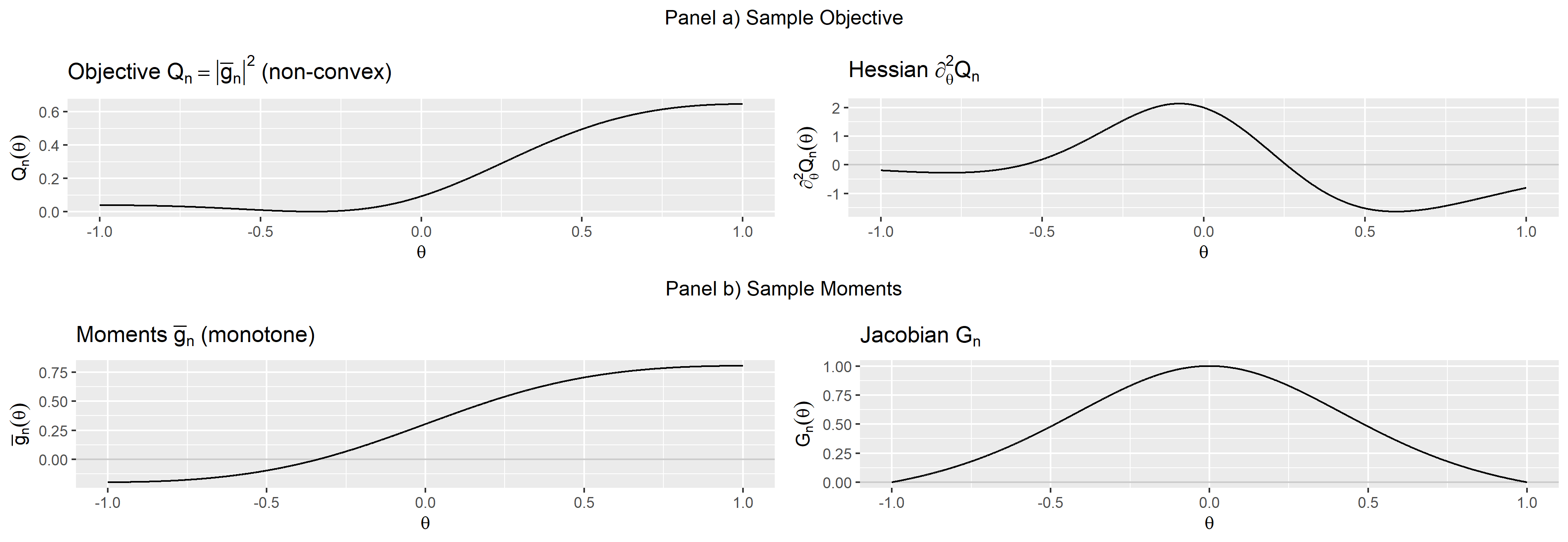
Figure 1: MA(1): illustration of non-convexity and the rank condition

Legend: simulated sample of size $n=200$, $\theta^{\dagger}=-1/2$, $\overline{g}_{n}(\theta)=\hat{\beta}_{1}-\theta/(1+\theta^{2})$, $W_{n}=I_{d}$. The GMM objective (panel a) is non-convex but the sample moments (panel b) satisfy the rank condition.

Table 2: MA(1): search paths for nr, gn, bfgs, and l-bfgs-b

$k$	0	1	2	3	4	5	6	7	8	…	99
	$p=1$
nr	-0.600	-0.689	-0.722	-0.749	-0.772	-0.793	-0.811	-0.828	-0.843	…	-0.993
gn	-0.600	-0.560	-0.529	-0.504	-0.484	-0.466	-0.451	-0.438	-0.427	…	-0.338
bfgs	-0.600	-0.505	4.425	-0.307	-0.359	-0.338	-0.337	-0.337	-0.337	…	-0.337
l-bfgs-b	-0.600	-0.505	1.000	-0.455	-0.375	-0.318	-0.341	-0.339	-0.338	…	-0.338
bfgs⋆	-0.600	-0.462	-0.286	-0.345	-0.340	-0.338	-0.338	-0.338	-0.338	…	-0.338
l-bfgs-b⋆	-0.600	-0.462	-0.286	-0.345	-0.339	-0.338	-0.338	-0.338	-0.338	…	-0.338
	$p=12$
nr	0.950	0.956	0.961	0.965	0.969	0.972	0.975	0.978	0.980	…	1.000
gn	0.950	0.890	0.860	0.834	0.810	0.787	0.763	0.740	0.715	…	-0.623
bfgs	0.950	-8.290	-8.279	-8.267	-8.256	-8.244	-8.233	-8.221	-8.209	…	-6.979
l-bfgs-b	0.950	-1.000	-1.000	-1.000	-1.000	-1.000	-1.000	-1.000	-1.000	…	-1.000

Legend: simulated data with sample size $n=200$, $\theta^{\dagger}=-1/2$. For $p=1$, $\overline{g}_{n}(\theta)=\hat{\beta}_{1}-\theta/(1+\theta^{2})$. For $p=12$, $\overline{g}_{n}(\theta)=\hat{\beta}_{n}-\beta(\theta)$ where $\beta(\theta)$ is the p-limit of the AR(p) coefficients, evaluated at $\theta$. $W_{n}=I_{d}$. The solutions are $\hat{\theta}_{n}=-0.339$ ($p=1$) and $\hat{\theta}_{n}=-0.626$ ($p=12$). nr = Newton-Raphson, gn = Gauss-Newton. The learning rate is $\gamma=0.1$ for nr and gn. bfgs = R’s optim, l-bfgs-b = R’s optim with bound constraints $\theta\in[-1,1]$. bfgs^⋆ and l-bfgs-b^⋆ apply the same optimizers to $F_{n}$ instead of $Q_{n}$. Additional results for gn using a range of values $\gamma\in\{0.1,0.2,0.4,0.6,0.8,1\}$ can be found in Appendix C.1, Figures C7, C10.

For $p=12$, the model becomes over-identified, and the condition for global convergence requires $G_{n}(\theta_{1})^{\prime}W_{n}G_{n}(\theta_{2})$ to be non-singular for all pairs $(\theta_{1},\theta_{2})\in\Theta\times\Theta$. For just-identified models, this amounts to $G_{n}(\theta)$ non-singular for all $\theta\in\Theta$. Figure C8 in Appendix C illustrates, similar to Figure 1, that $Q_{n}$ is non-convex and that the rank condition holds for $\Theta=[-1+\varepsilon,1-\varepsilon]$. $F_{n}$ is not defined because of over-identification. Table 2 shows that nr, bfgs and l-bfgs-b all fail to converge from $\theta_{0}=0.95$, a starting value with negative curvature. Compare with gn, which steadily converges to $\hat{\theta}_{n}$. Starting closer to the solution, bfgs and l-bfgs-b also fail to converge using $\theta_{0}=0.6$; gn remains accurate (not reported). R code to replicate the results with $p=12$, $W_{n}=I_{d}$ can be found in Appendix B.

3.1 Correctly-specified models

The first set of results concerns models that are correctly specified: the minimizer $\hat{\theta}_{n}$ is such that $\overline{g}_{n}(\hat{\theta}_{n})=O_{p}(n^{-1/2})$. The following Proposition shows that for any tuning parameter $\gamma$, there exists a neighborhood where (1) is locally convergent.

Proposition 1 (Local Convergence).

If Assumptions 1-2 hold, then for $\gamma\in(0,1)$ small enough, there exist $R_{n}\geq 0$ and $\tilde{\gamma}\in(0,1)$ such that with probability approaching $1$:

$$\|\theta_{k+1}-\hat{\theta}_{n}\|\leq(1-\tilde{\gamma})\|\theta_{k}-\hat{\theta}_{n}\|\leq\dots\leq(1-\tilde{\gamma})^{k+1}\|\theta_{0}-\hat{\theta}_{n}\|$$ (2)

for any $\|\theta_{0}-\hat{\theta}_{n}\|\leq R_{n}$. For just-identified models, $\overline{g}_{n}(\hat{\theta}_{n})=0$, $R_{n}>0$ with probability $1$. For over-identified models, $\overline{g}_{n}(\hat{\theta}_{n})=O_{p}(n^{-1/2})$, $R_{n}>0$ with probability approaching $1$.

A proof specialized to gn, and the general case are given in Appendix A. For gn, $R_{n}=\min(R_{G},\tilde{R}_{n})$ is the smallest of $R_{G}$ and:

$$\tilde{R}_{n}=(1-\tilde{\gamma}/\gamma)\frac{\underline{\sigma}}{L\sqrt{\kappa_{W}}}-\frac{1}{\underline{\sigma}\sqrt{\underline{\lambda}_{W}}}\|\overline{g}_{n}(\hat{\theta}_{n})\|_{W_{n}},$$

where $\kappa_{W}=\overline{\lambda}_{W}/\underline{\lambda}_{W}$ bounds the condition number of the weighting matrix $W_{n}$. Having $\|\overline{g}_{n}(\hat{\theta}_{n})\|_{W_{n}}\neq 0$ reduces the area of local convergence. For correctly specified models $\overline{g}_{n}(\hat{\theta}_{n})=O_{p}(n^{-1/2})$ implies $\tilde{R}_{n}\overset{p}{\to}\tilde{R}=(1-\tilde{\gamma}/\gamma)\underline{\sigma}\sqrt{\kappa_{W}}/L>0$. Note that for gn, Proposition 1 holds for any choice of $\gamma\in(0,1)$. This is typically not the case for other choices of $P_{k}$: gd is only locally convergent when $\gamma$ is sufficiently small. gd and gn iterations require the same inputs $G_{n}$ and $\overline{g}_{n}$, but the latter is preferred since it converges more quickly. Because nr and qn iterations require the exact and an approximate Hessian, they are more costly than gd, gn.

3.1.1 Just-Identified Models

The Theorem below proves global convergence for $\gamma\in(0,1)$ sufficiently small – under additional restrictions on $G_{n}$.

Theorem 1 (Global Convergence, Just-Identified).

Suppose $\overline{g}_{n}(\hat{\theta}_{n})=0$, Assumptions 1-2 hold, and with probability approaching $1$:

$$\sigma_{\min}[G_{n}(\theta)]\geq\underline{\sigma}>0,\,\forall\theta\in\Theta.$$ (3)

Then for $\gamma$ small enough, there exist a $\overline{\gamma}\in(0,1)$, and constants $0<\underline{\lambda}\leq\overline{\lambda}<\infty$ such that:

$$\|\theta_{k+1}-\hat{\theta}_{n}\|\leq(1-\overline{\gamma})^{k+1}\sqrt{\overline{\lambda}/\underline{\lambda}}\|\theta_{0}-\hat{\theta}_{n}\|,$$ (4)

for any starting value $\theta_{0}\in\Theta$, with probability approaching $1$.

The proof is given in Appendix A. The main steps are to show that for $\gamma$ sufficiently small, we have: i) $Q_{n}(\theta_{k+1})\leq(1-\overline{\gamma})^{2}Q_{n}(\theta_{k})$ for some $\overline{\gamma}\in(0,1)$ under condition (3) and Assumptions 1-2. Iterating on this inequality implies convergence of the objective function: $Q_{n}(\theta_{k})\leq(1-\overline{\gamma})^{2k}Q_{n}(\theta_{0})$. The same assumptions also imply the norm equivalence: ii) $\underline{\lambda}\|\theta-\hat{\theta}_{n}\|^{2}\leq Q_{n}(\theta)\leq\overline{\lambda}\|\theta-\hat{\theta}_{n}\|^{2}$ for some $0<\underline{\lambda}\leq\overline{\lambda}<+\infty$. Together, these two properties imply convergence of $\theta_{k}$ to $\hat{\theta}_{n}$.

The main takeaway from Theorem 1 is that global convergence can be achieved using any Algorithm which has $P_{k}$ strictly positive definite for any $k\geq 0$, with an adequate choice of $\gamma\in(0,1)$, if $G_{n}$ is everywhere non-singular. This assumption does not imply the convexity of $Q_{n}$. Note that the choice of $\gamma$ depends on the choice of algorithm, through $P_{k}$. Some methods are associated with faster convergence than others, which is measured by $\overline{\gamma}$. The following discusses the assumptions and the implications for the choice of algorithm.

Discussion of the rank condition.

In the scalar case, where both $\theta$ and $\overline{g}_{n}$ are one-dimensional, continuity of $G_{n}$ and the rank condition (3) implies that $\overline{g}_{n}$ is strictly monotone, i.e. injective. However, this does not imply that $Q_{n}$ is convex, as illustrated with the MA(1) example above. Under strict monotonicity, univariate methods such as bisection or golden-search converge at a similar rate but do not extend to multivariate estimations.

In the multivariate case, (3) implies a unique solution since $0=\overline{g}_{n}(\theta)=G_{n}(\tilde{\theta}_{n})(\theta-\hat{\theta}_{n})\Leftrightarrow\theta=\hat{\theta}_{n}$, for an intermediate value $\tilde{\theta}_{n}$. It further implies that $Q_{n}$ has no local minimum, besides $\hat{\theta}_{n}$, since $\partial_{\theta}Q_{n}(\theta)=G_{n}(\theta)^{\prime}W_{n}\overline{g}_{n}(\theta)=0\Leftrightarrow\overline{g}_{n}(\theta)=0\Leftrightarrow\theta=\hat{\theta}_{n}$, for just-identified models.

Unlike convexity, the assumption is invariant to one-to-one non-linear reparameterizations. Take any $h(\vartheta)=\theta$ where $\partial_{\vartheta}h(\vartheta)$ has full rank for all $\vartheta\in h^{-1}(\Theta)$. Consider the reparameterized sample moments $\overline{g}_{n}\circ h(\vartheta)$. The Jacobian $\partial_{\vartheta}\overline{g}_{n}\circ h(\vartheta)=G_{n}\circ h(\vartheta)\times\partial_{\vartheta}h(\vartheta)$ has full rank if, and only if, $G_{n}$ has full rank. Hence, (3) is primitive to the model and the choice of moments since it is not parameterization specific, unlike convexity.

It is also possible to have $Q_{n}$ convex without (3). Take $\overline{g}_{n}(\theta)=(\bar{y}_{n}-\theta)^{3}$, then $G_{n}(\theta)=0$ at $\hat{\theta}_{n}=\bar{y}_{n}$ - the rank condition does not hold, even locally. Yet, $Q_{n}(\theta)=(\bar{y}_{n}-\theta)^{6}$ is globally (non-strictly) convex. Condition (3) fails because $\hat{\theta}_{n}=\bar{y}_{n}$ is not a regular point (Rothenberg, 1971, Def4), i.e. $G_{n}$ does not have constant rank around $\hat{\theta}_{n}$. For the same counter-example, a gn update has the form: $\theta_{k+1}=\theta_{k}+\gamma/3(\bar{y}_{n}-\theta_{k})$ which converges exponentially fast to $\hat{\theta}_{n}=\bar{y}_{n}$ for any $\gamma\in(0,1]$ with $(1-\overline{\gamma})=(1-\gamma/3)$. Even though (3) fails, gn remains globally convergent with a fast rate. Hence, the condition is sufficient but not necessary.

Choice of Algorithm.

The conditioning matrix $P_{k}$ must be finite and strictly positive definite for all $k\geq 0$. This is always the case for gd since $P_{k}=I_{d}$ for all $k$. When $G_{n}$ has full rank everywhere, gn also satisfies the assumption since $P_{k}=[G_{n}(\theta_{k})^{\prime}W_{n}G_{n}(\theta_{k})]^{-1}$. However, if $Q_{n}$ is non-convex, then $\partial^{2}_{\theta,\theta^{\prime}}Q_{n}$ can be singular, and $P_{k}$ used in nr and qn may not be finite. This can negate the convergence result, as the MA(1) example illustrates.

When the rank condition (3) fails, Assumption 2 does not holds for gn but remains valid for gd. One could apply the Levenberg-Marquardt (LM) algorithm by setting $P_{k}=(G_{n}(\theta_{k})^{\prime}W_{n}G_{n}(\theta_{k})+\lambda I_{d})^{-1}$, and Assumption 2 holds for any $\lambda>0$. Global convergence is not guaranteed, however, since non-global local optima may exist when (3) does not hold.

Theorem 1 is related to solving just-identified non-linear systems of equations, here of the form: $\overline{g}_{n}(\theta)=0$. This is less studied than non-linear optimization. Dennis and Schnabel (1996) cast the problem as of minimizing $Q_{n}$, using the present notation, and derive global convergence results to a local minimum (Theorems 6.3.3-6.3.4). Deuflhard (2005, Ch3) gives conditions for convergence to a global solution. However, these results require an exact solution $\overline{g}_{n}(\hat{\theta}_{n})=0$ and, as discussed below, (3) may not suffice under over-identification.

3.1.2 Over-Identified Models

Theorem 2 (Global Convergence, Over-Identified).

Suppose $\overline{g}_{n}(\hat{\theta}_{n})=O_{p}(n^{-1/2})$, Assumptions 1-2, and for some $\rho\in(0,1]$, with probability approaching $1$:

$$\sigma_{\min}[G_{n}(\theta_{1})^{\prime}W_{n}G_{n}(\theta_{2})]\geq\rho\underline{\sigma}^{2}\underline{\lambda}_{W}>0,\forall(\theta_{1},\theta_{2})\in\Theta\times\Theta.$$ (3’)

Then for $\gamma$ small enough, there exist $\overline{\gamma}\in(0,1)$, $C>0$, $0<\underline{\lambda}\leq\overline{\lambda}<\infty$, and $C_{n}=O_{p}(1)$ such that with probability approaching $1$:

$$\|\theta_{k}-\hat{\theta}_{n}\|^{2}\leq (1-\overline{\gamma})^{2k}\frac{\overline{\lambda}+C\|\overline{g}_{n}(\hat{\theta}_{n})\|_{W_{n}}}{\underline{\lambda}-C\|\overline{g}_{n}(\hat{\theta}_{n})\|_{W_{n}}}\|\theta_{0}-\hat{\theta}_{n}\|^{2}+C_{n}\|\overline{g}_{n}(\hat{\theta}_{n})\|_{W_{n}}^{2},$$ (5)

for any $\theta_{0}\in\Theta$. Given this choice of $\gamma$, take $R_{n}$ from Proposition 1. Since $C_{n}\|\overline{g}_{n}(\hat{\theta}_{n})\|_{W_{n}}^{2}\leq R_{n}^{2}/2$ with probability approaching $1$, setting $k=k_{n}+j$, $j\geq 0$ implies:

$$\|\theta_{k}-\hat{\theta}_{n}\|\leq(1-\tilde{\gamma})^{j}R_{n},$$

where $\tilde{\gamma}\in(0,1)$ is the local rate in Proposition 1 and $k_{n}\geq\frac{2\log(R_{n})-\log 2-\log(d_{0n})}{2\log(1-\overline{\gamma})}$ with $d_{0n}=2[\underline{\lambda}-C\|\overline{g}_{n}(\hat{\theta}_{n})\|_{W_{n}}]^{-1}[\|\overline{g}_{n}(\theta_{0})\|^{2}_{W_{n}}-\|\overline{g}_{n}(\hat{\theta}_{n})\|^{2}_{W_{n}}]$.

The explicit formula for $\underline{\lambda},\overline{\lambda},C$, and $C_{n}$ are given in the proof of the Theorem (Appendix A). As discussed earlier, conditions (3) and (3’) are equivalent for just-identified models, when $W_{n}$ has full rank. Notice that larger values of $\|\overline{g}_{n}(\hat{\theta}_{n})\|_{W_{n}}$ can degrade convergence. The results for misspecified models will investigate the robustness of the results when $\|\overline{g}_{n}(\hat{\theta}_{n})\|_{W_{n}}$ does not vanish in the limit.

Condition (3’) extends the monotonicity condition found in the scalar case. When $\overline{g}_{n}$ and $\theta$ are both scalar, $\overline{g}_{n}$ is strictly increasing (or decreasing) only if $\partial_{\theta}\overline{g}_{n}(\theta_{1})\partial_{\theta}\overline{g}_{n}(\theta_{2})\neq 0$ for all $\theta_{1},\theta_{2}$; the derivative does not change sign. Here the condition reads as $\partial_{\theta}\overline{g}_{n}(\theta_{1})^{\prime}W_{n}\partial_{\theta}\overline{g}_{n}(\theta_{2})$ non-singular for $\theta_{1},\theta_{2}$. With the continuity of the Jacobian, this yields (3’) for some $\rho\in(0,1]$. Hence (3’) could be interpreted as a multivariate strict monotonicity condition on $W_{n}^{1/2}\overline{g}_{n}(\cdot)$.

To give some intuition why (3) in Theorem 1 alone may not suffice when the model is over-identified, consider the population problem $g(\theta)=0$. Suppose $G(\theta)$ has full rank for all $\theta\in\Theta$. Suppose $\theta$ is a local optimum: $G(\theta)^{\prime}Wg(\theta)=0$, then it is a fixed point of (1). Global convergence can only hold if $\theta=\theta^{\dagger}$ is the only fixed point. Using $g(\theta^{\dagger})=0$, write $G(\theta)^{\prime}W[g(\theta)-g(\theta^{\dagger})]=0=G(\theta)^{\prime}WG(\tilde{\theta})[\theta-\theta^{\dagger}]$, for some intermediate value $\tilde{\theta}$. This implies that if $G(\theta)^{\prime}WG(\tilde{\theta})$ has full rank then $\theta$ satisfies the first-order condition only if $\theta=\theta^{\dagger}$. Because the matrix $G(\theta)$ is rectangular for over-identified models, $(\ref{eq:rk})$ is not sufficient to rule out $G(\theta)^{\prime}WG(\tilde{\theta})$ singular, and thus the existence of local optima. Notice that (3’) could be weakened to: $G(\theta)^{\prime}WG(\tilde{\theta})$ has full rank for all $\theta\in\Theta$ and intermediate values $\tilde{\theta}=\omega\theta+(1-\omega)\theta^{\dagger}$, $\omega\in(0,1).$ Likewise, Theorem 2 could be derived assuming (3’) only for $\theta_{1}\in\Theta$ and $\theta_{2}=\omega\theta_{1}+(1-\omega)\hat{\theta}_{n}$, $\omega\in(0,1)$ since the derivations also involve intermediate values. The following explains why (3’) is preferred.

Condition (3’) is invariant to one-to-one non-linear reparameterization since $\partial_{\vartheta}\overline{g}_{n}\circ h(\vartheta)=G_{n}\circ h(\vartheta)\times\partial_{\vartheta}h(\vartheta)$ and (3’) becomes $\partial_{\vartheta}h(\vartheta_{1})^{\prime}G_{n}\circ h(\vartheta_{1})^{\prime}W_{n}G_{n}\circ h(\vartheta_{2})\partial_{\vartheta}h(\vartheta_{2})$ which has full rank if $G_{n}\circ h(\vartheta_{1})^{\prime}W_{n}G_{n}\circ h(\vartheta_{2})$ has full rank for all $h(\vartheta_{1})$, $h(\vartheta_{2})$ given that $\partial_{\vartheta}h(\vartheta_{1}),\partial_{\vartheta}h(\vartheta_{2})$ are full rank square matrices. The weaker version of (3’) discussed above would not be invariant to non-linear reparameterizations since $h(\omega\vartheta+(1-\omega)\hat{\vartheta}_{n})$ need not be an intermediate value between $h(\vartheta)$ and $h(\hat{\vartheta}_{n})$ for a non-linear $h(\cdot)$.

Condition (3’) is not invariant to the choice of $W_{n}$. Appendix C illustrates that the condition may hold for some $W_{n}$ (Figure C8) but not for another (Figure C9). This is perhaps not surprising as changes in $W_{n}$ can alter the null space of $G_{n}(\theta_{1})^{\prime}W_{n}^{1/2}$.

Another pen and pencil example.

Take $y_{i}\sim\mathcal{N}(\mu,\sigma^{2})$, the parameters of interest are $\theta=(\mu,\sigma^{2})$. Compute the sample moments $\hat{\mu}_{n}=(\hat{\mu}_{n1},\hat{\mu}_{n2},\hat{\mu}_{n4})^{\prime}$, where $\hat{\mu}_{n1}=\overline{y}_{n}$, $\hat{\mu}_{n2}=\hat{\sigma}_{n}^{2}$, and $\hat{\mu}_{n4}=1/n\sum_{i=1}^{n}(y_{i}-\overline{y}_{n})^{4}$, and let: $\overline{g}_{n}(\theta)=\hat{\mu}_{n}-(\mu,\sigma^{2},3\sigma^{4})$. Set $W_{n}=I_{d}$ and take $\theta^{\dagger}=(0,1)$. A quick numerical computation reveals the population objective function is non-convex: the eigenvalues of $\partial_{\theta,\theta^{\prime}}^{2}Q(\theta)$ are $(74,2)$ at $\theta=(0,1)$ and $(2,-7)$ at $\theta=(0,1/2)$ – the Hessian is positive definite at the true value but not everywhere. For starting values such that $\partial_{\theta,\theta^{\prime}}^{2}Q_{n}(\theta)$ is (near)-singular, nr and qn iterations can be erratic, as in the MA(1) example. Nonetheless, condition (3’) holds since:

$$G_{n}(\theta)^{\prime}=\left(\begin{array}[]{ccc}-1&0&0\\ 0&-1&-6\sigma^{2}\end{array}\right),\quad G_{n}(\theta_{1})^{\prime}G_{n}(\theta_{2})=\left(\begin{array}[]{cc}1&0\\ 0&1+36\sigma_{1}^{2}\sigma_{2}^{2}\end{array}\right)$$

is positive definite for any two $\theta_{1}=(\mu_{1},\sigma_{1}^{2})$, $\theta_{2}=(\mu_{2},\sigma_{2}^{2})$ with $\sigma_{1},\sigma_{2}\geq 0$. In this simple example, the Hessian of $Q_{n}$ can be singular, yet condition (3’) holds globally.

Much like convexity, condition (3’) can be challenging to verify analytically for more complex models. Still, it can be evaluated numerically on a grid, as illustrated for the MA(1) model in Figure C8, Appendix C. Unlike just-identified models, condition (3’) does not immediately exclude local optima in finite samples. Still, the following Proposition shows that all local optima $\theta_{n}$ are asymptotically valid estimators, i.e. $\sqrt{n}(\theta_{n}-\hat{\theta}_{n})=o_{p}(1)$.

Proposition 2 (Local optima are asymptotically valid estimators).

Suppose Assumption 1 and (3’) hold. If $\|\overline{g}_{n}(\hat{\theta}_{n})\|_{W_{n}}=O_{p}(n^{-1/2})$, then for any $\theta_{n}$ such that $G_{n}(\theta_{n})^{\prime}W_{n}\overline{g}_{n}(\theta_{n})=0$:

$$\|\theta_{n}-\hat{\theta}_{n}\|\leq\overline{C}\|\overline{g}_{n}(\hat{\theta}_{n})\|^{2}_{W_{n}}=O_{p}(n^{-1}),$$

where $\overline{C}>0$ only depends on $G_{n}$ and $W_{n}$.

Proposition 1 implies local convergence to $\hat{\theta}_{n}$. And yet, Proposition 2 alone does not exclude the presence of local optima $\theta_{n}$ near $\hat{\theta}_{n}$ to which (1) could converge. These two results are not at odds, however. Proposition 2 and local convexity imply: $\theta_{n}=\hat{\theta}_{n}$ with probability approaching $1$. The following sketches the argument. Take $\theta_{n}$, a local optimum: $\partial_{\theta}Q_{n}(\theta_{n})=0$ and $\|\tilde{\theta}_{n}-\hat{\theta}_{n}\|\leq O_{p}(n^{-1})$, by Proposition 2. Then $0=\partial_{\theta}Q_{n}(\theta_{n})(\theta_{n}-\hat{\theta}_{n})=(\theta_{n}-\hat{\theta}_{n})^{\prime}\partial^{2}_{\theta,\theta^{\prime}}Q_{n}(\tilde{\theta}_{n})(\theta_{n}-\hat{\theta}_{n})\geq\lambda_{\min}[\partial^{2}_{\theta,\theta^{\prime}}Q_{n}(\tilde{\theta}_{n})]\|\theta_{n}-\hat{\theta}_{n}\|^{2}$ for an intermediate value $\tilde{\theta}_{n}$. Also, $\partial^{2}_{\theta,\theta^{\prime}}Q_{n}(\tilde{\theta}_{n})=\partial^{2}_{\theta,\theta^{\prime}}Q_{n}(\hat{\theta}_{n})+o_{p}(1)=G_{n}(\hat{\theta}_{n})^{\prime}W_{n}G_{n}(\hat{\theta}_{n})+o_{p}(1)$, by continuity, for correctly specified models. This implies $\lambda_{\min}[\partial^{2}_{\theta,\theta^{\prime}}Q_{n}(\tilde{\theta}_{n})]>0$, strictly, with probability approaching $1$. As desired, we have that $\|\theta_{n}-\hat{\theta}_{n}\|=0$ with probability approaching $1$.

3.2 Misspecified models

So far, the results imply that fast global convergence is feasible under a rank condition for correctly specified models. In applications, misspecification can be a concern so that understanding the robustness of the results above to non-negligible deviations from this baseline is empirically relevant. Recently, Hansen and Lee (2021) studied the properties of iterated GMM procedures. Here the focus is on computing a single GMM estimate. The following considers “moderate” amounts of misspecification in the sense that:

$$\text{plim}_{n\to\infty}Q_{n}(\hat{\theta}_{n}):=\varphi^{2}\geq 0$$

exists and can be non-zero in the limit. When $\varphi>0$, the degree of misspecification is non-negligible asymptotically and, with optimal weighting, the J-statistic $n\|\overline{g}_{n}(\hat{\theta}_{n})\|_{W_{n}}^{2}\to\infty$ can diverge. However, $\varphi$ cannot be too large for the local and global convergence results to hold as shown below. For simplicity, only Gauss-Newton will be considered in the results. Also, since $G_{n}$ cannot be full rank at $\theta=\hat{\theta}_{n}$ when the model is both just-identified and misspecified, the results presented here solely consider over-identified models.

For correctly specified models, an over-identification test can diagnose global convergence (Andrews, 1997, Sec3.3). For misspecified models, such test would frequently reject in large samples. Then the issue is that, when the test rejects, either 1) the estimates are not valid, or 2) the model fits the data poorly in some dimension(s). When $Q_{n}$ is globally convex, the estimates are the global solution if, and only if, they satisfy the first and second order optimality conditions. Without convexity, this only guarantees a local optimum. Here, checking the rank condition (3’), as in Figure C7, helps determine whether global convergence is at risk, or not, which is the main concern when $Q_{n}(\hat{\theta}_{n})$ is significantly non-zero.

Proposition 3 (Local Convergence, Misspecified).

Suppose Assumptions 1-2 hold, and $\varphi$ is such that:

$$0\leq\varphi<\frac{\underline{\sigma}^{2}\underline{\lambda}_{W}}{L\overline{\lambda}_{W}^{1/2}}.$$ (6)

For any $\gamma\in(0,1)$, there exists $\tilde{\gamma}\in(0,\gamma)$, such that, with probability approaching $1$, for some $R_{n}>0$, strictly positive, any $\|\theta_{0}-\hat{\theta}_{n}\|\leq R_{n}$, and all $k\geq 0$:

$$\|\theta_{k+1}-\hat{\theta}_{n}\|\leq(1-\tilde{\gamma})\|\theta_{k}-\hat{\theta}_{n}\|\leq\dots\leq(1-\tilde{\gamma})^{k+1}\|\theta_{0}-\hat{\theta}_{n}\|.$$ (2’)

Also, $\text{plim}_{n\to\infty}R_{n}=R>0$.

$R_{n}$ in Proposition 3 takes the same form as in Proposition 1, (6) ensures that the corresponding $R$ is strictly positive in the limit; the neighborhood of convergence is non-negligible asymptotically. Under identity weighting, $W_{n}=I_{d}$, (6) only depends on $\underline{\sigma}$ and $L$. For linear models, $L=0$ implies that any $\varphi\in[0,\infty)$ is feasible. For non-linear models, a larger $L>0$ requires a smaller $\varphi$: increased non-linearity requires milder misspecification. Smaller values of $\underline{\sigma}$, which measures local identification, also require a smaller $\varphi$. In Proposition 1 with gn, any rate of convergence $\overline{\gamma}\in(0,\gamma)$ can be used. When the model is misspecified, larger values of $\varphi\geq 0$ require $\tilde{\gamma}\in(0,\gamma)$ to be sufficiently small.

Theorem 3 (Global Convergence, Misspecified).

Suppose Assumptions 1-2 and (3’) hold. If $\varphi$ is such that:

$$0\leq\varphi<\frac{\underline{\sigma}^{2}\underline{\lambda}_{W}}{2L\overline{\lambda}_{W}^{1/2}}.$$ (6’)

Then for $\gamma$ small enough, there exist $\overline{\gamma}\in(0,1)$ and $C_{n}=O_{p}(1)$, $0<C,\underline{\lambda},\overline{\lambda}<\infty$, which do not depend on $\varphi$, such that with probability approaching $1$:

$$\|\theta_{k}-\hat{\theta}_{n}\|^{2}\leq (1-\overline{\gamma})^{2k}\frac{\overline{\lambda}+C\|\overline{g}_{n}(\hat{\theta}_{n})\|_{W_{n}}}{\underline{\lambda}-C\|\overline{g}_{n}(\hat{\theta}_{n})\|_{W_{n}}}\|\theta_{0}-\hat{\theta}_{n}\|^{2}+C_{n}\|\overline{g}_{n}(\hat{\theta}_{n})\|_{W_{n}}^{2}.$$ (5’)

Let $\Delta=1/2[\underline{\sigma}^{2}\underline{\lambda}_{W}-2L\overline{\lambda}_{W}^{1/2}\varphi]>0$. Suppose $\gamma\in(0,1)$ and $\varphi\geq 0$ are such that:

$$\frac{\Delta\gamma^{2}c_{2}+2\gamma\overline{c}^{2}_{3}/\underline{c}_{1}}{[\gamma\underline{c}_{1}/2-\gamma^{2}c_{2}]\Delta^{2}}\varphi^{2}<\left((1-\varepsilon)\frac{\underline{\sigma}}{L\sqrt{\kappa}_{W}}-\frac{\varphi}{\underline{\sigma}\sqrt{\underline{\lambda}_{W}}}\right)^{2},$$ (7)

for some $\varepsilon\in(0,1)$, where $\underline{c}_{1}=2/3\rho^{2}([\underline{\sigma}/\overline{\sigma}]^{2}\kappa^{-1}_{W})^{2}$, $c_{2}=L_{Q}(\overline{\sigma}\overline{\lambda}_{W}^{1/2}/[\underline{\sigma}^{2}\underline{\lambda}_{W}])^{2}$, $\overline{c}_{3}=2\overline{\sigma}\overline{\lambda}^{1/2}_{W}$, $\kappa_{W}=\overline{\lambda}_{W}/\underline{\lambda}_{W}$, and $L_{Q}$ is the Lipschitz constant of $\partial_{\theta}Q_{n}$. Take any $\tilde{\gamma}\in(0,\varepsilon\gamma)$ and $R_{n}$ from Proposition 3, set $k=k_{n}+j$, $j\geq 0$, then with probability approaching $1$:

$$\|\theta_{k}-\hat{\theta}_{n}\|\leq(1-\tilde{\gamma})^{j}R_{n},$$

where $k_{n}\geq\frac{2\log(R_{n})+\log(\delta)-\log(d_{0n})}{2\log(1-\overline{\gamma})}$, with $d_{0n}$ as in Theorem 2, for some small enough $\delta\in(0,1)$.

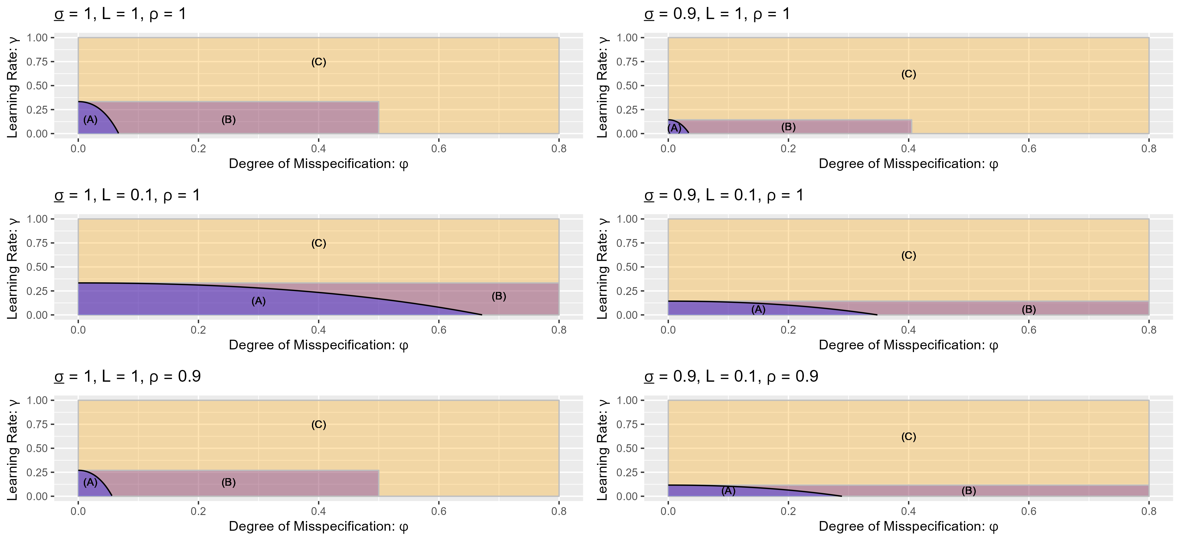
Figure 2: Illustration of the conditions for $(\gamma,\varphi)$ in Theorem 3

Legend: (A) all 3 conditions hold, (B) condition (7) does not hold, (C) all conditions fail. Black curve: upper bound for (7). Figure drawn using $\overline{\sigma}=1,W_{n}=I_{d},L_{Q}=1$, and $\varepsilon=10^{-4}.$

Theorem 3 above shows that for “moderate” amounts of misspecification, gn remains globally convergent for an appropriate choice of tuning parameter $\gamma\in(0,1)$. Three conditions are required for the result to hold: (6’) bounds $\varphi$ from above; (5’) bounds $\gamma$ from above – independently of $\varphi$. Condition (7) restricts the pair $(\gamma,\varphi)$ to prove convergence to the global solution. Figure 2 illustrates the 3 conditions and the effect $\underline{\sigma}$, $L$, and $\rho$ have on the feasible set for $(\gamma,\varphi)$. Everything else held equal, a smaller value of $\underline{\sigma}$ or $\rho$ shrinks the feasible set. A smaller $L$, implies less non-linearity, offsets these two and expands the feasible set for $\varphi$. Generally, larger values of $\varphi$ restrict the learning rate $\gamma$ to be smaller.

4 Empirical Applications

4.1 Estimation of a Random Coefficient Demand Model Revisited

The following revisits the results for random coefficient demand estimation in Knittel and Metaxoglou (2014) with the cereal data from Nevo (2001). This is a non-linear instrumental variable regression with sample moment conditions: $\overline{g}_{n}(\theta,\beta)=\frac{1}{n}\sum_{j,t}z_{jt}[\delta_{jt}(\theta)-x_{tj}^{\prime}\beta]$, where $z_{jt}$ are the instruments, $x_{jt}$ the linear regressors in market $j$ at time period $t$. The $8$ parameters of interest are the random coefficients $\theta$, which enter $\delta_{jt}$, recovered from market shares $s_{jt}$ using the fixed point algorithm of Berry et al. (1995). The $25$ linear coefficients $\beta$ are nuisance parameters concentrated out by two-stage least squares for each $\theta$.

Table 3: Demand for Cereal: performance comparison

		stdev				income				objs	# of
		const.	price	sugar	mushy	const.	price	sugar	mushy		crashes
true	est	0.28	2.03	-0.01	-0.08	3.58	0.47	-0.17	0.69	33.84	-
	se	0.11	0.76	0.01	0.15	0.56	3.06	0.02	0.26	-
	avg	0.28	2.03	-0.01	-0.08	3.58	0.47	-0.17	0.69	33.84
gn	std	0.00	0.00	0.00	0.00	0.00	0.00	0.00	0.00	0.00	0
bfgs	avg	0.28	2.03	-0.01	-0.08	3.58	0.47	-0.17	0.69	33.84	30
	std	0.00	0.00	0.00	0.00	0.01	0.00	0.00	0.00	0.00
nm	avg	0.32	0.35	-0.08	-0.88	3.94	-2.64	-0.10	1.26	628.44	4
	std	1.37	8.91	0.09	3.08	3.63	10.74	0.23	5.13	772.23
sa	avg	0.87	-0.58	-0.72	-0.00	0.01	0.33	1.64	-1.16	$1.46\cdot 10^{5}$	3
	std	7.68	8.66	3.58	7.88	6.67	6.97	3.65	7.92	$2.36\cdot 10^{5}$
sa+nm	avg	0.43	-0.88	-0.06	-0.84	4.15	-2.18	-0.15	0.71	506.44	3
	std	0.61	9.45	0.12	2.25	3.56	11.48	0.19	5.06	1250.65

Legend: Comparison for 50 starting values in $[-10,10]\times\dots\times[-10,10]$. Avg, Std: sample average and standard deviation of optimizer outputs. true: full sample estimate (est) and standard errors (se). Objs: avg and std of minimized objective value. # of crashes: optimization terminated because the objective function returned an error. gn run with $\gamma=0.1$ for $k=150$ iterations for all starting values. Additional results for gn using a range of values $\gamma\in\{0.1,0.2,0.4,0.6,0.8,1\}$ can be found in Appendix C.2, Table C5.

Table 3 and Figure 3 compare the performance of quasi-Newton (bfgs), Nelder-Mead (nm), Simulated-Annealing (sa), and Nelder-Mead after Simulated-Annealing (sa+nm), using R’s default optimizer optim, with Gauss-Newton (gn) for 50 different starting values. As reported in Knittel and Metaxoglou (2014), optimization can crash often. Crashes could be avoided using error handling (try-catch statements). However, this may not be enough to produce accurate estimates as the next application will illustrate. Only gn and bfgs systematically produce accurate estimates, but bfgs crashes 60% of the time. Derivative-free optimizers, nm, sa, and sa+nm, can produce inaccurate estimates.

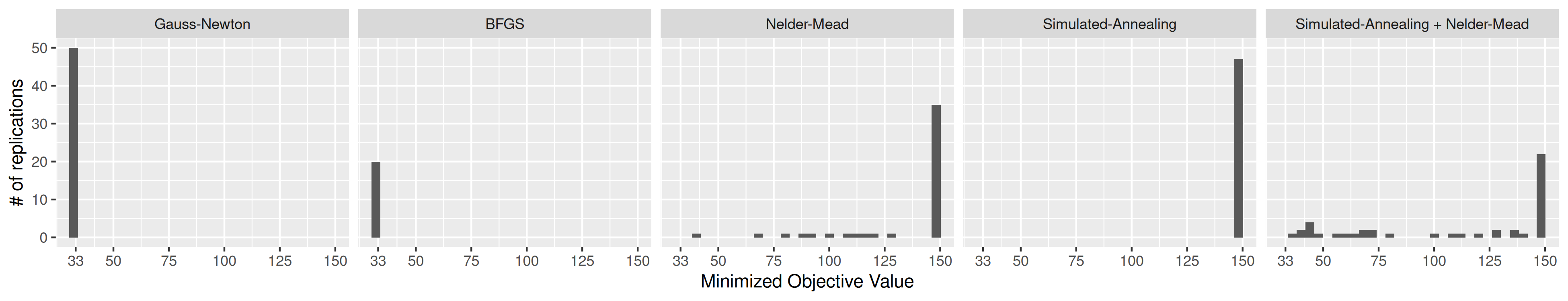
Figure 3: Demand for Cereal: distribution of minimized objective values

Legend: Comparison for 50 starting values. Minimized objective values for non-crashed optimizations. Objective values are truncated from above at $Q_{n}(\theta)=150$.

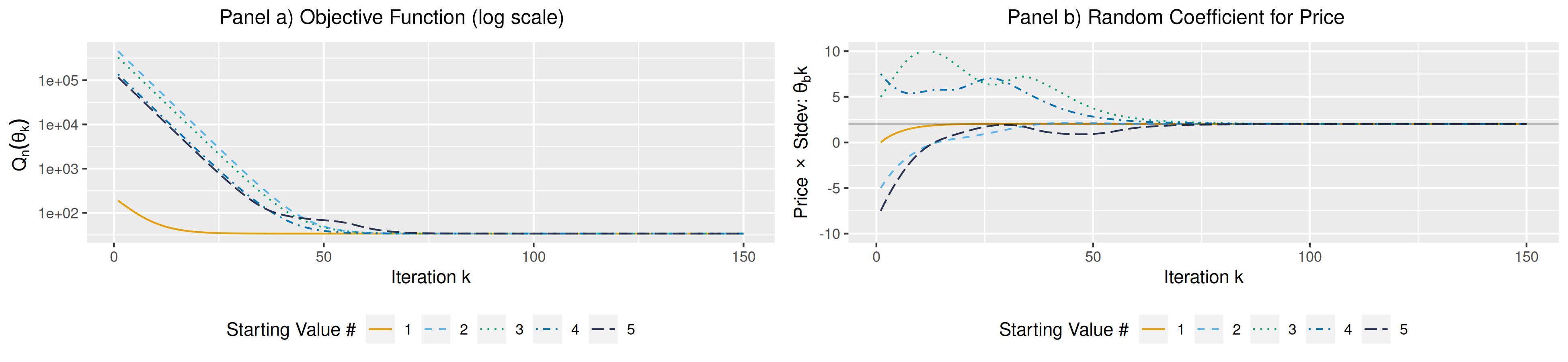
Figure 4: Demand for Cereal: Gauss-Newton iterations for 5 starting values

Legend: 150 gn iterations for 5 starting values in $[-10,10]\times\dots\times[-10,10]$. Panel b) horizontal grey line = full sample estimate.

Figure 4, illustrates the convergence of gn for the first 5 starting values. In line with the predictions of Theorem 2, though $Q_{n}$ is non-convex, gn iterations steadily converge to the solution. This type of “Gauss-Newton regression” is related to Salanié and Wolak (2022) who compute a two-stage least-squares estimate of a linear approximation of the BLP random coefficient model.

4.2 Innovation, Productivity, and Monetary Policy

The second application revisits Moran and Queralto (2018)’s estimation of a model with endogenous total factor productivity (TFP) growth (see Moran and Queralto, 2018, Sec2, for details about the model). They estimate parameters related to Research and Development (R&D) by matching the impulse response function (IRF) of an identified R&D shock to R&D and TFP in a small-scale Vector Auto-Regression (VAR) estimated on U.S. data.

The parameters of interest are $\theta=(\eta,\nu,\rho_{s},\sigma_{s})$ which measure, respectively, the elasticity of technology creation to R&D, R&D spillover to adoption, the persistence coefficient and size of impulse to the R&D wedge. The sample moments are $\overline{g}_{n}(\theta)=\hat{\psi}_{n}-\psi(\theta)$, $\hat{\psi}_{n}$ and $\psi(\theta)$ are the sample and predicted IRFs, respectively. The latter is computed using Dynare in Matlab. To minimize $Q_{n}$, the authors use Sims’s csminwel algorithm with a reparameterization which bounds the coefficients. This type of reparameterization is commonly used, however its yields a near-singular Jacobian near the boundary which can affect both local and global convergence, according to the results.

Table 4: Impulse Response Matching: performance comparison

		$\eta$	$\nu$	$\rho_{s}$	$\sigma_{s}$	objs	# of crashes
true	est	0.30	0.29	0.39	0.17	4.65	-
without reparameterization
	avg	0.30	0.29	0.39	0.17	4.65
gn	std	0.00	0.00	0.00	0.00	0.00	2
bfgs	avg	0.12	0.10	-0.34	5.42	$2.23\cdot 10^{4}$	0
	std	0.56	0.20	0.47	4.77	$2.31\cdot 10^{4}$
csminwel	avg	0.36	-0.00	0.27	0.15	46.42	0
	std	0.24	1.54	0.33	0.19	183.74
nm	avg	0.47	-5.27	0.43	0.16	14.81	0
	std	0.54	37.28	0.11	0.05	34.32
sa	avg	1.39	-2.08	0.48	0.09	75.21	0
	std	2.23	3.59	0.19	0.09	91.35
sa+nm	avg	0.97	-84.27	0.41	0.09	66.53	0
	std	2.01	124.00	0.22	0.09	79.78
with reparameterization
	avg	0.30	0.29	0.39	0.17	4.65
gn	std	0.00	0.00	0.00	0.00	0.00	5
bfgs	avg	0.37	0.21	0.07	0.14	104.08	0
	std	0.32	0.14	0.65	0.06	136.63
csminwel	avg	0.62	0.20	0.07	0.14	133.76	0
	std	0.39	0.22	0.76	0.08	123.32
nm	avg	0.48	0.26	0.37	0.39	$1.29\cdot 10^{3}$	0
	std	0.33	0.16	0.34	1.68	$8.92\cdot 10^{3}$
sa	avg	0.60	0.21	0.44	1.26	$6.93\cdot 10^{3}$	0
	std	0.46	0.30	0.74	3.62	$2.06\cdot 10^{4}$
sa+nm	avg	0.61	0.21	0.43	1.08	$5.41\cdot 10^{3}$	2
	std	0.45	0.29	0.71	3.33	$1.76\cdot 10^{4}$
lower bound		0.05	0.01	-0.95	0.01	-	-
upper bound		0.99	0.90	0.95	12	-	-

Legend: Comparison for 50 starting values. true: full sample estimate (est). Objs: avg and std of minimized objective value. # of crashes: optimization terminated because objective returned error. Lower/upper bound used for the reparameterization. gn run with $\gamma=0.1$ for $k=150$ iterations for all starting values. Standard errors were not computed in the original study. Additional results for gn, using a range of values $\gamma\in\{0.1,0.2,0.4,0.6,0.8,1\}$ can be found in Appendix C.3, Tables C6, C7

In the original paper, the authors intialize the estimation at $\theta_{0}=(\eta_{0},\nu_{0},\rho_{s0},\sigma_{s0})=(0.20,0.20,0.30,0.10)$, very close to $\hat{\theta}_{n}$. Here, 50 starting values are generated, within the bounds in Table 4. The model is estimated using csminwel and the same set of optimizers used in the previous replication. Table 4 reports the results with and without the non-linear reparameterization. Similar to the MA(1) model with $p=12$, without the reparameterization, several optimizers return values outside the parameter bounds which motivates the contraints in these cases. gn correctly estimates the parameters for all starting values but crashes twice for starting values for which both $\eta$ and $\nu$ are close to their lower bounds where the Jacobian is nearly singular. With the reparameterization, gn crashed more often, five times in total, but is otherwise accurate. The other two gradient-based optimizers, bfgs and csminwel, never crash because of better error handling in Matlab. They do encounter a number values where the model cannot be solved in Dynare, which then returns an error. This suggests they produce inaccurate search directions. They produce valid estimates less often than gn. Figure 5 illustrates that csminwel is sensitive to reparameterization. Likewise, derivative-free methods can be inaccurate, as illustrated in Table 4 and Figure 5; some crashes occur despite Matlab’s error handling. Finally, Figure 6 shows 5 optimization paths for which gn does not crash with and without the reparameterization. They are nearly identical. Tables C6, C7 in Appendix C.3 gives additional results for larger values of $\gamma\in(0,1]$, plus results with error handling and the global step from Forneron (2023).

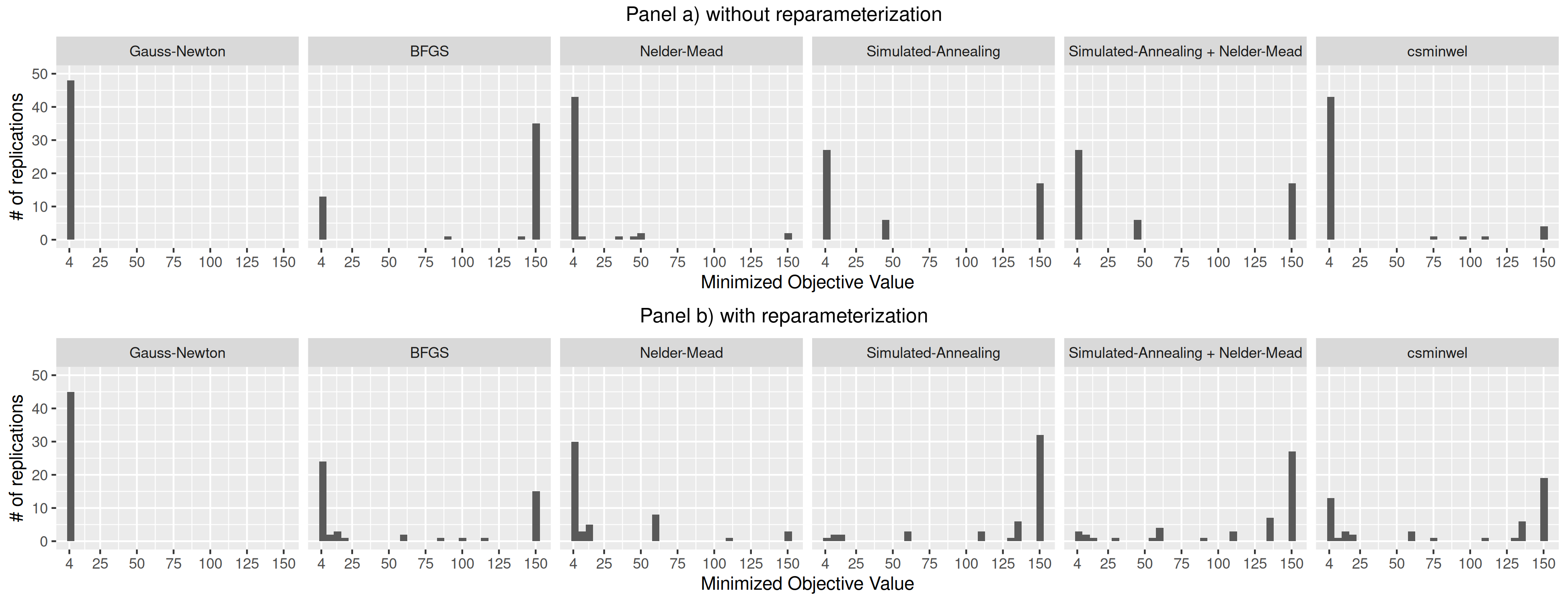
Figure 5: Impulse Response Matching: distribution of minimized objective values

Legend: Comparison for 50 starting values. Minimized objective values for non-crashed optimizations. Objective values are truncated from above at $Q_{n}(\theta)=150$.

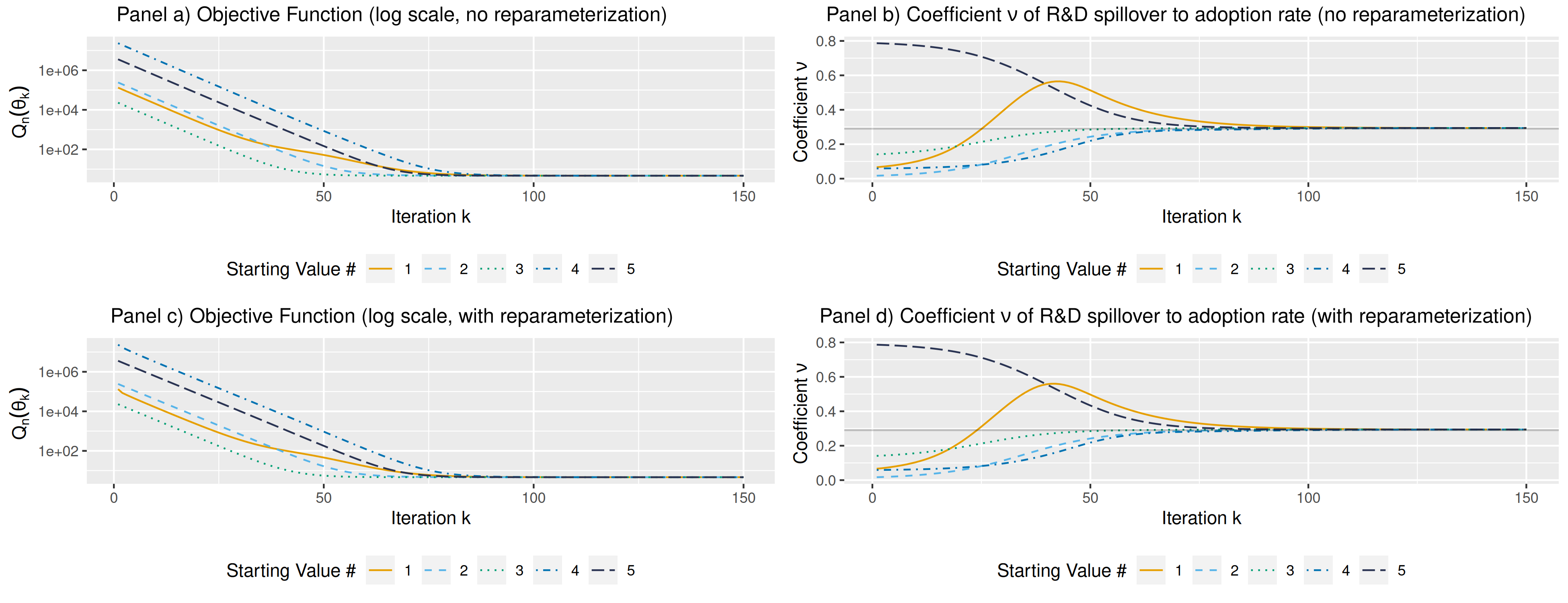
Figure 6: Impulse Response Matching: Gauss-Newton iterations for 5 starting values

Legend: 150 gn iterations for 5 non-crashing starting values. Panels a,c) value of the objective function at each iteration, Panels b,d) coefficient $\eta$ at each iteration; horizontal grey line = full sample estimate.

5 Conclusion

Non-convexity of the GMM objective function is an important challenge for structural estimation, and the survey highlights how practitioners approach this issue. This paper considers an alternative condition under which there are globally convergent algorithms. The results are robust to non-convexity, one-to-one non-linear reparameterizations, and moderate misspecification. Econometric theory emphasizes the role of the weighting matrix $W_{n}$ on the statistical efficiency of the estimator $\hat{\theta}_{n}$. Also, Hall and Inoue (2003), Hansen and Lee (2021) showed it can alter the pseudo-true value of the parameter under misspecification. Here, the rank condition (3’) may or may not hold, depending on $W_{n}$. The condition number $\kappa_{W}$ also affects local convergence. This highlights another role for the weighting matrix: it may facilitate or hinder the estimation itself. Two empirical applications illustrate the performance of the preferred Gauss-Newton algorithm.

Appendix A Proofs for the Main Results

A.1 Primitive Conditions for Assumption 1

In the following we will use the notation: $\overline{g}_{n}(\theta)=1/n\sum_{i=1}^{n}g(\theta;x_{i})$, $g(\theta)=\mathbb{E}[\overline{g}_{n}(\theta)]$, $G(\theta;x_{i})=\partial_{\theta}g(\theta;x_{i})$, $G_{n}(\theta)=1/n\sum_{i=1}^{n}G(\theta;x_{i})$, $G(\theta)=\mathbb{E}[G_{n}(\theta)]$, $Q_{n}(\theta)=\overline{g}_{n}(\theta)^{\prime}W_{n}\overline{g}_{n}(\theta)$, and $Q(\theta)=g(\theta)^{\prime}Wg(\theta)$. $W_{n}$ and $W$ are symmetric. With probability approaching 1 will be abbreviated as wpa1. $\mathcal{B}_{R}(\theta^{\dagger})$ is a closed ball of radius $R$, centered around $\theta^{\dagger}$.

Assumption A1.

Suppose the observations $x_{i}$ are iid and, for some $\delta\in(0,1)$: i. $Q(\theta)=\|g(\theta)\|^{2}_{W}$ has a unique minimum $\theta^{\dagger}\in\text{interior}(\Theta)$ such that $Q(\theta^{\dagger})=0$, $\mathbb{E}[\|g(\theta;x_{i})\|^{2}]<\infty$, for all $\theta\in\Theta$, ii. $g(\theta;x_{i})$ and $g(\theta)$ are twice continuously differentiable on $\Theta$, iii. $\mathbb{E}[\|G(\theta;x_{i})\|^{2}]<\infty$, for all $\theta\in\Theta$, there exist a $\bar{L}(\cdot)\geq 0$ such that for any $(\theta_{1},\theta_{2})\in\Theta^{2}$, $\|G(\theta_{1};x_{i})-G(\theta_{2};x_{i})\|\leq\bar{L}(x_{i})\|\theta_{1}-\theta_{2}\|$, where $\mathbb{E}[|\bar{L}(x_{i})|^{2}]<\infty$, and $\mathbb{E}[\bar{L}(x_{i})]\leq(1-\delta)L$, for some $R_{G}>0$ such that $\mathcal{B}_{(1+\delta)R_{G}}(\theta^{\dagger})\subseteq\Theta$, $\sigma_{\min}[G(\theta)]\geq(1+\delta)\underline{\sigma}>0$ for all $\|\theta-\theta^{\dagger}\|\leq(1+\delta)R_{G}$, iv. The parameters space $\Theta$ is convex and compact, and v. $W_{n}\overset{p}{\to}W$, $0<(1+\delta)\underline{\lambda}_{W}\leq\lambda_{\min}(W)\leq\lambda_{\max}(W)(1-\delta)\overline{\lambda}_{W}<\infty$.

Remarks.

The condition $Q(\theta^{\dagger})=0$ is only used to prove that the arg-minimizer $\hat{\theta}_{n}$ is unique wpa1. It could be relaxed to allow for moderate misspecification, at the cost of longer derivations and several bounds on the amount of misspecification $\varphi$, as in Theorem 3. The condition that $x_{i}$ are iid can also be weakened to allow for non-identically distributed dependent observations by appropriately adjusting the moment conditions in A1i, iii which are used to derive uniform laws of large numbers for $\overline{g}_{n}$ and $G_{n}$.

Lemma A1.

Assumption A1 implies Assumption 1.

Proof of Lemma A1.

Assumption 1ii, iv follow from A1ii, iv. Use Weyl’s perturbation inequality for singular values (Bhatia, 2013, Problem III.6.5) to find $\lambda_{\min}(W_{n})\geq\lambda_{\min}(W)-\sigma_{\max}(W_{n}-W)\geq(1+\delta)\underline{\lambda}_{W}-o_{p}(1)\geq\underline{\lambda}_{W}$, wpa 1. Likewise, $\lambda_{\max}(W_{n})\leq\overline{\lambda}_{W}$, wpa1. This yields Assumption 1v.

Assumption A1iii and compactness imply uniform convergence of the sample Jacobian $\sup_{\theta\in\Theta}\|G_{n}(\theta)-G(\theta)\|=o_{p}(1)$, see Jennrich (1969). We also have uniform convergence for the same moments. Condition ii implies $\overline{g}_{n}(\theta)-g(\theta)=o_{p}(1)$, for all $\theta$. Notice that $\|[\overline{g}_{n}(\theta_{1})-g(\theta_{1})]-[\overline{g}_{n}(\theta_{2})-g(\theta_{2})]\|=\|[G_{n}(\tilde{\theta})-G(\tilde{\theta})](\theta_{1}-\theta_{2})\|\leq[\sup_{\theta\in\Theta}\|G_{n}(\theta)-G(\theta)\|]\|\theta_{1}-\theta_{2}\|$, where the $\sup$ is a $o_{p}(1)$ by uniform convergence of $G_{n}$. Using a finite cover and arguments similar to Jennrich (1969), this implies uniform convergence: $\sup_{\theta\in\Theta}\|\overline{g}_{n}(\theta)-g(\theta)\|=o_{p}(1)$.

Then, uniform convergence of $\overline{g}_{n}$ and $W_{n}\overset{p}{\to}W$ imply uniform converge of $Q_{n}$ to $Q$. Continuity and the global identification condition A1i. imply $\hat{\theta}_{n}\overset{p}{\to}\theta^{\dagger}$ (Newey and McFadden, 1994, Th2.1). This implies that $\|\theta-\hat{\theta}_{n}\|\leq R_{G}\Rightarrow\|\theta-\theta^{\dagger}\|\leq R_{G}+o_{p}(1)\leq(1+\delta)R_{G}$, wpa 1, i.e. $\mathcal{B}_{R_{G}}(\hat{\theta}_{n})\subseteq\mathcal{B}_{(1+\delta)R_{G}}(\theta^{\dagger})\subseteq\Theta$. This implies $\hat{\theta}_{n}\in\text{interior}(\Theta)$, wpa1. Then, for the same $\theta$, $\sigma_{\min}[G(\theta)]\geq(1+\delta)\underline{\sigma}$, wpa1. Apply Weyl’s inequality for singular values to find that, uniformly in $\theta$: $\sigma_{\min}[G_{n}(\theta)]\geq\sigma_{\min}[G_{n}(\theta)]-\sigma_{\max}[G(\theta)-G_{n}(\theta)]\geq(1+\delta)\underline{\sigma}-o_{p}(1)\geq\underline{\sigma}>0$, wpa 1. Take any two $\theta_{1},\theta_{2}$ in $\Theta$, $\|G_{n}(\theta_{1})-G_{n}(\theta_{2})\|\leq 1/n\sum_{i=1}^{n}\bar{L}(x_{i})\|\theta_{1}-\theta_{2}\|\leq[(1+\delta)L+o_{p}(1)]\|\theta_{1}-\theta_{2}\|\leq L\|\theta_{1}-\theta_{2}\|$, wpa1, using a law of large numbers for $\bar{L}(x_{i})$. This yields all the conditions in Assumption 1iii.

Remains to show that the sample arg-minimizer $\hat{\theta}_{n}$ is unique, wpa1, so that Assumption 1i also holds. Having shown that Assumption 1ii-v holds, we can use it in the following. Using the same steps as in the beginning of the proof of Theorem 2:

$$(\underline{\lambda}-C\|\overline{g}_{n}(\hat{\theta}_{n})\|_{W_{n}})\|\theta-\hat{\theta}_{n}\|^{2}\leq 2[Q_{n}(\theta)-Q_{n}(\hat{\theta}_{n})],$$

wpa1, but here only locally, i.e. uniformly in $\|\theta-\hat{\theta}_{n}\|\leq R_{G}$. Any approximate minimizer is in this neighborhood wpa1, by consistency, so we only need to check the unicity of an exact minimizer within this neighborhood.

We have $\underline{\lambda}=\min_{\|\theta-\hat{\theta}_{n}\|\leq R_{G}}\lambda_{\min}(G_{n}(\theta)^{\prime}W_{n}G_{n}(\theta))\geq\underline{\sigma}^{2}\underline{\lambda}_{W}$, wpa1, and $C:=2\sqrt{\lambda_{\max}(W_{n})}L$, bounded wpa1 as well. Now $Q_{n}(\hat{\theta}_{n})=o_{p}(1)$ by uniform convergence and A1i, $Q(\theta^{\dagger})=0$, likewise $(\underline{\lambda}-C\|\overline{g}_{n}(\hat{\theta}_{n})\|_{W_{n}})\geq 1/2\underline{\lambda}>0$, wpa1. Take $\hat{\theta}_{n}$ to be an exact minimizer, and any $\theta\neq\hat{\theta}_{n}$ such that $\|\theta-\hat{\theta}_{n}\|\leq R_{G}$, then $Q_{n}(\theta)\geq Q_{n}(\hat{\theta}_{n})+1/4\underline{\lambda}\|\theta-\hat{\theta}_{n}\|^{2}>Q_{n}(\hat{\theta}_{n})$, wpa1. This implies that the arg-minimizer $\hat{\theta}_{n}$ is unique wpa1 and concludes the proof. ∎

A.2 Proofs for Section 3.1

Proof of Proposition 1 (Gauss-Newton).

Take $\theta_{k}\in\Theta$, the update (1) can be re-written as:

$$\theta_{k+1}-\hat{\theta}_{n}= \Big{(}I_{d}-\gamma P_{k}G_{n}(\theta_{k})^{\prime}W_{n}G_{n}(\theta_{k})\Big{)}(\theta_{k}-\hat{\theta}_{n})$$ (A.1)

$$-\gamma P_{k}G_{n}(\theta_{k})^{\prime}W_{n}[\overline{g}_{n}(\theta_{k})-G_{n}(\theta_{k})(\theta_{k}-\hat{\theta}_{n})].$$

For gn, $P_{k}G_{n}(\theta_{k})^{\prime}W_{n}G_{n}(\theta_{k})\ =I_{d}$ so that we have:

$$\theta_{k+1}-\hat{\theta}_{n}= (1-\gamma)(\theta_{k}-\hat{\theta}_{n})$$ (A.1’)

$$-\gamma P_{k}G_{n}(\theta_{k})^{\prime}W_{n}[\overline{g}_{n}(\theta_{k})-\overline{g}_{n}(\hat{\theta}_{n})-G_{n}(\theta_{k})(\theta_{k}-\hat{\theta}_{n})]$$

$$-\gamma P_{k}[G_{n}(\theta_{k})-G_{n}(\hat{\theta}_{n})]^{\prime}W_{n}\overline{g}_{n}(\hat{\theta}_{n}),$$

using the first-order condition $G_{n}(\hat{\theta}_{n})^{\prime}W_{n}\overline{g}_{n}(\hat{\theta}_{n})=0$. From Assumption 1, there exists $R_{G}>0$ such that: $\underline{\sigma}\leq\sigma_{\min}[G_{n}(\theta_{k})]$ for any $\|\theta_{k}-\hat{\theta}_{n}\|\leq R_{G}$, which implies that $P_{k}$ is well defined and bounded. Since $G_{n}$ is Lipschitz continuous with constant $L\geq 0$:

$$\|P_{k}G_{n}(\theta_{k})^{\prime}W_{n}[\overline{g}_{n}(\theta_{k})-\overline{g}_{n}(\hat{\theta}_{n})-G_{n}(\theta_{k})(\theta_{k}-\hat{\theta}_{n})]\|\leq\underline{\sigma}^{-1}\sqrt{\overline{\lambda}_{W}/\underline{\lambda}_{W}}L\|\theta_{k}-\hat{\theta}_{n}\|^{2},$$

We also have:

$$\|P_{k}[G_{n}(\theta_{k})-G_{n}(\hat{\theta}_{n})]^{\prime}W_{n}\overline{g}_{n}(\hat{\theta}_{n})\|\leq\underline{\sigma}^{-2}(\sqrt{\overline{\lambda}_{W}}/\underline{\lambda}_{W})L\|\overline{g}_{n}(\hat{\theta}_{n})\|_{W_{n}}\|\theta_{k}-\hat{\theta}_{n}\|.$$

Combine these two inequalities into (A.1’) to find:

$$\|\theta_{k+1}-\hat{\theta}_{n}\|$$ (A.1”)

$$\leq\left(1-\gamma+\gamma\left[\underline{\sigma}^{-1}\sqrt{\overline{\lambda}_{W}/\underline{\lambda}_{W}}L\|\theta_{k}-\hat{\theta}_{n}\|+\underline{\sigma}^{-2}(\sqrt{\overline{\lambda}_{W}}/\underline{\lambda}_{W})L\|\overline{g}_{n}(\hat{\theta}_{n})\|_{W_{n}}\right]\right)\|\theta_{k}-\hat{\theta}_{n}\|.$$

Now take any $\tilde{\gamma}\in(0,\gamma)$, let:

$$\tilde{R}_{n}=\frac{\gamma-\tilde{\gamma}}{\gamma}\left[L^{-1}\underline{\sigma}\sqrt{\underline{\lambda}_{W}/\overline{\lambda}_{W}}\right]-(\underline{\sigma}^{-1}/\sqrt{\underline{\lambda}_{W}})\|\overline{g}_{n}(\hat{\theta}_{n})\|_{W_{n}}.$$

Let $R_{n}=\min(\tilde{R}_{n},R_{G})$, for any $\|\theta_{k}-\hat{\theta}_{n}\|\leq R_{n}$, we have $\|\theta_{k+1}-\hat{\theta}_{n}\|\leq(1-\tilde{\gamma})\|\theta_{k}-\hat{\theta}_{n}\|\leq R_{n}$. By recursion, we then have for any $\|\theta_{0}-\hat{\theta}_{n}\|\leq R_{n}$:

$$\|\theta_{k+1}-\hat{\theta}_{n}\|\leq(1-\tilde{\gamma})\|\theta_{k}-\hat{\theta}_{n}\|\leq\dots\leq(1-\tilde{\gamma})^{k+1}\|\theta_{0}-\hat{\theta}_{n}\|,$$

as stated in (2). ∎

Proof of Proposition 1 (General Case).

Take $\theta_{k}\in\Theta$, the update (1) can be re-written as:

$$\theta_{k+1}-\hat{\theta}_{n}= \Big{(}I_{d}-\gamma P_{k}G_{n}(\theta_{k})^{\prime}W_{n}G_{n}(\theta_{k})\Big{)}(\theta_{k}-\hat{\theta}_{n})$$ (A.1)

$$-\gamma P_{k}G_{n}(\theta_{k})^{\prime}W_{n}[\overline{g}_{n}(\theta_{k})-G_{n}(\theta_{k})(\theta_{k}-\hat{\theta}_{n})].$$

Taking norms on both sides this identity yields:

$$\|\theta_{b+1}-\hat{\theta}_{n}\|\leq \sigma_{\max}\Big{[}I_{d}-\gamma P_{k}G_{n}(\theta_{k})^{\prime}W_{n}G_{n}(\theta_{k})\Big{]}\|\theta_{b}-\hat{\theta}_{n}\|$$ (A.1’)

$$+\gamma\|P_{k}G_{n}(\theta_{k})^{\prime}W_{n}[\overline{g}_{n}(\theta_{k})-G_{n}(\theta_{k})(\theta_{k}-\hat{\theta}_{n})]\|,$$

where $\sigma_{\max}$ returns the largest singular value. We will now bound each of these two terms. First, note that $\sigma_{\max}[I_{d}-\gamma P_{k}G_{n}(\theta_{k})^{\prime}W_{n}G_{n}(\theta_{k})]=\sigma_{\max}[I_{d}-\gamma P_{k}^{1/2}G_{n}(\theta_{k})^{\prime}W_{n}G_{n}(\theta_{k})P_{k}^{1/2}]=\max_{j=1,\dots,d}|\lambda_{j}[I_{d}-\gamma P_{k}^{1/2}G_{n}(\theta_{k})^{\prime}W_{n}G_{n}(\theta_{k})P_{k}^{1/2}]|$, where $\lambda_{j}$ are the eigenvalues. Because this is a difference of Hermitian matrices, Weyl’s perturbation inequality (Bhatia, 2013, Corollary III.2.2) implies the following bounds:

$$1-\gamma\lambda_{\max}[P_{k}^{1/2}G_{n}(\theta_{k})^{\prime}W_{n}G_{n}(\theta_{k})P_{k}^{1/2}] \leq\lambda_{\min}[I_{d}-\gamma P_{k}^{1/2}G_{n}(\theta_{k})^{\prime}W_{n}G_{n}(\theta_{k})P_{k}^{1/2}]$$

$$\leq\lambda_{\max}[I_{d}-\gamma P_{k}^{1/2}G_{n}(\theta_{k})^{\prime}W_{n}G_{n}(\theta_{k})P_{k}^{1/2}]$$

$$\leq 1-\gamma\lambda_{\min}[P_{k}^{1/2}G_{n}(\theta_{k})^{\prime}W_{n}G_{n}(\theta_{k})P_{k}^{1/2}].$$

Let $\overline{\sigma}=\max_{\theta\in\Theta}\sigma_{\max}[G_{n}(\theta)]$, suppose $0<\gamma<[\overline{\lambda}_{P}\overline{\lambda}_{W}\overline{\sigma}^{2}]^{-1}$, we then have:

$$0\leq 1-\gamma\lambda_{\max}[P_{k}^{1/2}G_{n}(\theta_{k})^{\prime}W_{n}G_{n}(\theta_{k})P_{k}^{1/2}]\leq 1-\gamma\lambda_{\min}[P_{k}^{1/2}G_{n}(\theta_{k})^{\prime}W_{n}G_{n}(\theta_{k})P_{k}^{1/2}],$$

so that we are only concerned with the upper bound. From Assumption 1, $\|\theta-\hat{\theta}_{n}\|\leq R_{G}\Rightarrow\sigma_{\min}[G_{n}(\theta)]\geq\underline{\sigma}$. Combine with the bound for $\gamma$ to find:

$$0\leq\sigma_{\max}[I_{d}-\gamma P_{k}G_{n}(\theta_{k})^{\prime}W_{n}G_{n}(\theta_{k})]\leq 1-\gamma\underline{\lambda}_{P}\underline{\lambda}_{W}\underline{\sigma}^{2}<1,$$

for any choice of $\gamma\in(0,[\overline{\lambda}_{P}\overline{\lambda}_{W}\overline{\sigma}^{2}]^{-1})$. For the second term in (A.1), using the identity $G_{n}(\hat{\theta}_{n})^{\prime}W_{n}\overline{g}_{n}(\hat{\theta}_{n})=0$ and the mean value Theorem, we have for some intermediate value $\tilde{\theta}_{k}$:

$$P_{k}G_{n}(\theta_{k})^{\prime}W_{n}[\overline{g}_{n}(\theta_{k})-G_{n}(\theta_{k})(\theta_{k}-\hat{\theta}_{n})]= P_{k}G_{n}(\theta_{k})^{\prime}W_{n}[G_{n}(\tilde{\theta}_{k})-G_{n}(\theta_{k})](\theta_{k}-\hat{\theta}_{n})$$

$$+P_{k}[G_{n}(\theta_{k})-G_{n}(\hat{\theta}_{n})]^{\prime}W_{n}\overline{g}_{n}(\hat{\theta}_{n}).$$

Since $G_{n}$ is Lipschitz continuous with constant $L\geq 0$:

$$\|(\ref{eq:update2}^{\prime})\| \leq(1-\gamma\underline{\lambda}_{P}\underline{\lambda}_{W}\underline{\sigma}^{2})\|\theta_{b}-\hat{\theta}_{n}\|+\gamma\overline{\lambda}_{P}\overline{\lambda}_{W}\overline{\sigma}L\|\theta_{b}-\hat{\theta}_{n}\|^{2}+\gamma\overline{\lambda}_{P}\overline{\lambda}_{W}^{1/2}L\|\overline{g}_{n}(\hat{\theta}_{n})\|_{W_{n}}\|\theta_{b}-\hat{\theta}_{n}\|$$

$$=\Big{(}1-\gamma\underline{\lambda}_{P}\underline{\lambda}_{W}\underline{\sigma}^{2}+\gamma\Big{[}\overline{\lambda}_{P}\overline{\lambda}_{W}\overline{\sigma}L\|\theta_{b}-\hat{\theta}_{n}\|+\overline{\lambda}_{P}\overline{\lambda}_{W}^{1/2}L\|\overline{g}_{n}(\hat{\theta}_{n})\|_{W_{n}}\Big{]}\Big{)}\|\theta_{b}-\hat{\theta}_{n}\|.$$

Let $c_{1}=\overline{\lambda}_{P}\overline{\lambda}_{W}\overline{\sigma}L$, $c_{2}=\overline{\lambda}_{P}\overline{\lambda}_{W}^{1/2}L$, pick $\tilde{\gamma}\in(0,\gamma\underline{\lambda}_{P}\underline{\lambda}_{W}\underline{\sigma}^{2})$, and assume:

$$\|\theta_{k}-\hat{\theta}_{n}\|\leq\frac{\gamma\underline{\lambda}_{P}\underline{\lambda}_{W}\underline{\sigma}^{2}-\tilde{\gamma}}{\gamma c_{1}}-\frac{c_{2}}{c_{1}}\|\overline{g}_{n}(\hat{\theta}_{n})\|_{W_{n}}:=\tilde{R}_{n}.$$ (A.2)

Take $R_{n}=\min(R_{G},\tilde{R}_{n})$, $\|\theta_{k}-\hat{\theta}_{n}\|\leq R_{n}$ implies that, by construction:

$$\|\theta_{k+1}-\hat{\theta}_{n}\|\leq(1-\tilde{\gamma})\|\theta_{k}-\hat{\theta}_{n}\|\leq\dots\leq(1-\overline{\gamma})^{k+1}\|\theta_{0}-\hat{\theta}_{n}\|,$$

by recursion, if $\|\theta_{0}-\hat{\theta}_{n}\|\leq R_{n}$. ∎

Proof of Theorem 1

In the just-identified case, we will repeatedly use the identities $\overline{g}_{n}(\hat{\theta}_{n})=0$ and $Q_{n}(\hat{\theta}_{n})=\frac{1}{2}\overline{g}_{n}(\hat{\theta}_{n})^{\prime}W_{n}\overline{g}_{n}(\hat{\theta}_{n})=0$. Take any $\theta\in\Theta$, by the Mean Value Theorem there is some $\tilde{\theta}_{n}$ between $\theta$ and $\hat{\theta}_{n}$ such that $\overline{g}_{n}(\theta)=G_{n}(\tilde{\theta}_{n})(\theta-\hat{\theta}_{n})$ which implies:

$$\left(\frac{1}{2}\min_{\theta\in\theta}\lambda_{\min}[G_{n}(\theta)^{\prime}W_{n}G_{n}(\theta)]\right)\|\theta-\hat{\theta}_{n}\|^{2}\leq Q_{n}(\theta)\leq\left(\frac{1}{2}\max_{\theta\in\theta}\lambda_{\max}[G_{n}(\theta)^{\prime}W_{n}G_{n}(\theta)]\right)\|\theta-\hat{\theta}_{n}\|^{2},$$

and, using the full rank assumption, let $0<\underline{\lambda}\leq\overline{\lambda}<\infty$, denote respectively the $\min$ and the $\max$. This yields an equivalence between the two distances $\|\theta-\hat{\theta}_{n}\|$ and $Q_{n}(\theta)$. Apply the Mean Value Theorem to $Q_{n}$, for some $\tilde{\theta}_{k}$ between $\theta_{k}$ and $\theta_{k+1}$ in (1):

$$Q_{n}(\theta_{k+1})=Q_{n}(\theta_{k})+\partial_{\theta}Q_{n}(\theta_{k})^{\prime}(\theta_{k+1}-\theta_{k})+[\partial_{\theta}Q_{n}(\tilde{\theta}_{k})-\partial_{\theta}Q_{n}(\theta_{k})]^{\prime}(\theta_{k+1}-\theta_{k}),$$ (A.3)

where $\partial_{\theta}Q_{n}(\theta_{k})=G_{n}(\theta_{k})^{\prime}W_{n}\overline{g}_{n}(\theta_{k})$ and $\theta_{k+1}-\theta_{k}=-\gamma P_{k}G_{n}(\theta_{k})^{\prime}W_{n}\overline{g}_{n}(\theta_{k})$. This yields a first inequality:

$$\partial_{\theta}Q_{n}(\theta_{k})^{\prime}(\theta_{k+1}-\theta_{k}) =-\gamma\overline{g}_{n}(\theta_{k})^{\prime}W_{n}^{1/2}\left(W_{n}^{1/2}G_{n}(\theta_{k})P_{k}G_{n}(\theta_{k})^{\prime}W_{n}^{1/2}\right)W_{n}^{1/2}\overline{g}_{n}(\theta_{k})$$

$$\leq-\gamma c_{1}\|\overline{g}_{n}(\theta_{k})\|_{W_{n}}^{2},$$

where $c_{1}:=\min_{\theta\in\Theta}\lambda_{\min}[W_{n}^{1/2}G_{n}(\theta)P_{k}G_{n}(\theta)^{\prime}W_{n}^{1/2}]>0$, using the full rank assumption, and $\|\overline{g}_{n}(\theta_{k})\|_{W_{n}}^{2}=Q_{n}(\theta_{k})$. For the second inequality, since $\overline{g}_{n}$ is twice continuously differentiable and $\Theta$ is compact, $\partial_{\theta}Q_{n}$ is Lipschitz continuous with constant $L_{Q}\geq 0$. This implies:

$$\|[\partial_{\theta}Q_{n}(\tilde{\theta}_{k})-\partial_{\theta}Q_{n}(\theta_{k})]^{\prime}(\theta_{k+1}-\theta_{k})\|\leq L_{Q}\|\tilde{\theta}_{k}-\theta_{k}\|\times\|\theta_{k+1}-\theta_{k}\| \leq L_{Q}\|\theta_{k+1}-\theta_{k}\|^{2}$$

$$\leq\gamma^{2}c_{2}\|\overline{g}_{n}(\theta_{k})\|_{W_{n}}^{2},$$

since $\|\theta_{k+1}-\theta_{k}\|=\gamma\|P_{k}G_{n}(\theta_{k})^{\prime}W_{n}\overline{g}_{n}(\theta_{k})\|$ and $\|\tilde{\theta}_{k}-\theta_{k}\|\leq\|\theta_{k+1}-\theta_{k}\|$, setting $c_{2}:=L_{Q}\max_{\theta\in\Theta}\sigma^{2}_{\max}[P_{k}G_{n}(\theta)^{\prime}W_{n}^{1/2}]<+\infty$. Combine the two inequalities into (A.3) to find:

$$Q_{n}(\theta_{k+1})\leq(1-\gamma c_{1}+\gamma^{2}c_{2})Q_{n}(\theta_{k}),$$

for any $\theta_{k}\in\Theta$. The polynomial $P(\gamma)=1-\gamma c_{1}+\gamma^{2}c_{2}$ is such that $P(0)=1,d_{\gamma}P(0)<0$ which implies $P(\gamma)\in(0,1)$ strictly for any $\gamma>0$ sufficiently small. Take any such $\gamma$ and let $(1-\overline{\gamma})^{2}=P(\gamma)\in(0,1)$ for some $\overline{\gamma}\in(0,1)$, by construction. Take any $\theta_{0}\in\Theta$, by recursion:

$$Q_{n}(\theta_{k+1})\leq(1-\overline{\gamma})^{2}Q_{n}(\theta_{k})\leq\dots\leq(1-\overline{\gamma})^{2(k+1)}Q_{n}(\theta_{0}).$$

Now apply the distance equivalence derived earlier to get the desired result:

$$\|\theta_{k+1}-\hat{\theta}_{n}\|\leq(1-\overline{\gamma})^{k+1}\sqrt{\overline{\lambda}/\underline{\lambda}}\|\theta_{0}-\hat{\theta}_{n}\|.$$

∎

Proof of Theorem 2.

The general layout of the proof is similar to the just-identified case. Differences arise because $Q_{n}(\hat{\theta}_{n})\neq 0$ in general and $G_{n}(\theta)$ only has rank $d_{\theta}$ which is less than the dimension of $\overline{g}_{n}$ so that several parts of the proof do not apply anymore. First:

$$Q_{n}(\theta)-Q_{n}(\hat{\theta}_{n})=\frac{1}{2}\left[\overline{g}_{n}(\theta)-\overline{g}_{n}(\hat{\theta}_{n})\right]^{\prime}W_{n}\left[\overline{g}_{n}(\theta)-\overline{g}_{n}(\hat{\theta}_{n})\right]+\left[\overline{g}_{n}(\theta)-\overline{g}_{n}(\hat{\theta}_{n})\right]^{\prime}W_{n}\overline{g}_{n}(\hat{\theta}_{n}).$$

The leading term equals $\frac{1}{2}(\theta-\hat{\theta}_{n})^{\prime}G_{n}(\tilde{\theta}_{n})^{\prime}W_{n}G_{n}(\tilde{\theta}_{n})(\theta-\hat{\theta}_{n})$ which can be bounded above and below using the same approach as before. For the last term, use the first-order condition $G_{n}(\hat{\theta}_{n})^{\prime}W_{n}\overline{g}_{n}(\hat{\theta}_{n})=0$ to get, using $\overline{g}_{n}(\theta)-\overline{g}_{n}(\hat{\theta}_{n})=[G(\tilde{\theta}_{n})-G_{n}(\hat{\theta}_{n})+G_{n}(\hat{\theta}_{n})](\theta-\hat{\theta}_{n})$:

$$\|[\overline{g}_{n}(\theta)-\overline{g}_{n}(\hat{\theta}_{n})]^{\prime}W_{n}\overline{g}_{n}(\hat{\theta}_{n})\| \leq\sqrt{\lambda_{\max}(W_{n})}\|\theta-\hat{\theta}_{n}\|\times\|G_{n}(\hat{\theta}_{n})-G_{n}(\tilde{\theta}_{n})\|\times\|\overline{g}_{n}(\hat{\theta}_{n})\|_{W_{n}}$$

$$\leq\sqrt{\lambda_{\max}(W_{n})}L\|\overline{g}_{n}(\hat{\theta}_{n})\|_{W_{n}}\|\theta-\hat{\theta}_{n}\|^{2},$$

where $L\geq 0$ is the Lipschitz constant of $G_{n}$. Let $0<\underline{\lambda}=\min_{\theta\in\Theta}\lambda_{\min}[G_{n}(\theta)^{\prime}W_{n}G_{n}(\theta)]\leq\overline{\lambda}=\max_{\theta\in\Theta}\lambda_{\max}[G_{n}(\theta)^{\prime}W_{n}G_{n}(\theta)]<\infty$, apply the triangular inequality and its reverse to find the relation:

$$\left(\underline{\lambda}-C\|\overline{g}_{n}(\hat{\theta}_{n})\|_{W_{n}}\right)\|\theta-\hat{\theta}_{n}\|^{2}\leq 2[Q_{n}(\theta)-Q_{n}(\hat{\theta}_{n})]\leq\left(\overline{\lambda}+C\|\overline{g}_{n}(\hat{\theta}_{n})\|_{W_{n}}\right)\|\theta-\hat{\theta}_{n}\|^{2},$$ (A.4)

where $C:=2\sqrt{\lambda_{\max}(W_{n})}L\geq 0$ is finite. As in the just-identified case, we can write:

$$Q_{n}(\theta_{k+1})=Q_{n}(\theta_{k})+\partial_{\theta}Q_{n}(\theta_{k})^{\prime}(\theta_{k+1}-\theta_{k})+[\partial_{\theta}Q_{n}(\tilde{\theta}_{k})-\partial_{\theta}Q_{n}(\theta_{k})]^{\prime}(\theta_{k+1}-\theta_{k}),$$

and bound each of the last two terms. As before, we have:

$$\partial_{\theta}Q_{n}(\theta_{k})^{\prime}(\theta_{k+1}-\theta_{k})=-\gamma\overline{g}_{n}(\theta_{k})^{\prime}W_{n}G_{n}(\theta_{k})P_{k}G_{n}(\theta_{k})^{\prime}W_{n}\overline{g}_{n}(\theta_{k}),$$

however $\text{dim}(W_{n}^{1/2}\overline{g}_{n}(\theta_{k}))>\text{rank}[W_{n}^{1/2}G_{n}(\theta_{k})P_{k}G_{n}(\theta_{k})^{\prime}W_{n}^{1/2}]$, the model being over-identified. Hence, we only have $\partial_{\theta}Q_{n}(\theta_{k})^{\prime}(\theta_{k+1}-\theta_{k})\leq 0$ which, unlike the just-identified case, does not imply a strict contraction. Nevertheless, we have $\overline{g}_{n}(\theta_{k})=G_{n}(\tilde{\theta}_{k})(\theta_{k}-\hat{\theta}_{n})+\overline{g}_{n}(\hat{\theta}_{n})$ where $\text{dim}(\theta_{k}-\hat{\theta}_{n})$ equals the rank of the matrix above. Let $A_{k}=W_{n}^{1/2}G_{n}(\theta_{k})P_{k}G_{n}(\theta_{k})^{\prime}W_{n}^{1/2}$:

$$-\gamma\overline{g}_{n}(\theta_{k})^{\prime}W_{n}G_{n}(\theta_{k}) P_{k}G_{n}(\theta_{k})^{\prime}W_{n}\overline{g}_{n}(\theta_{k})$$

$$= -\gamma\left[\overline{g}_{n}(\theta_{k})-\overline{g}_{n}(\hat{\theta}_{n})\right]^{\prime}W_{n}^{1/2}A_{k}W_{n}^{1/2}\left[\overline{g}_{n}(\theta_{k})-\overline{g}_{n}(\hat{\theta}_{n})\right]$$ (A.5)

$$-\gamma\overline{g}_{n}(\hat{\theta}_{n})^{\prime}W_{n}^{1/2}A_{k}W_{n}^{1/2}\overline{g}_{n}(\hat{\theta}_{n})$$ (A.6)

$$-2\gamma\overline{g}_{n}(\hat{\theta}_{n})^{\prime}W_{n}^{1/2}A_{k}W_{n}^{1/2}\left[\overline{g}_{n}(\theta_{k})-\overline{g}_{n}(\hat{\theta}_{n})\right].$$ (A.7)

Now, bound these terms one at a time:

$$(\ref{eq:1}) =-\gamma(\theta_{k}-\hat{\theta}_{n})^{\prime}G_{n}(\tilde{\theta}_{k})^{\prime}W_{n}^{1/2}A_{k}W_{n}^{1/2}G_{n}(\tilde{\theta}_{k})(\theta_{k}-\hat{\theta}_{n})$$

$$\leq-\gamma\|\theta_{k}-\hat{\theta}_{n}\|^{2}\min_{\theta\in\Theta}\lambda_{\min}[G_{n}(\theta)^{\prime}W_{n}^{1/2}A_{k}W_{n}^{1/2}G_{n}(\theta)]$$

$$\leq-\gamma c_{1n}[Q_{n}(\theta_{k})-Q_{n}(\hat{\theta}_{n})],$$

where the last inequality comes from (A.4) above, and

$$c_{1n}:=\min_{\theta\in\Theta}\lambda_{\min}[G_{n}(\theta)^{\prime}W_{n}^{1/2}A_{k}W_{n}^{1/2}G_{n}(\theta)](\overline{\lambda}/2+C/2\|\overline{g}_{n}(\hat{\theta}_{n})\|_{W_{n}})^{-1}>0,$$

is bounded below by a strictly positive value with probability approaching 1, using Assumption 2 and condition (3’). To see why condition (3’) is critical, notice that $G_{n}(\theta)^{\prime}W_{n}^{1/2}A_{k}W_{n}^{1/2}G_{n}(\theta)=G_{n}(\theta)^{\prime}W_{n}G_{n}(\theta_{k})P_{k}G_{n}(\theta_{k})^{\prime}W_{n}G_{n}(\theta)$ is symmetric and has full rank if both $G_{n}(\theta)^{\prime}W_{n}G_{n}(\theta_{k})$ and $P_{k}$ have full rank. Both condition (3’) and Assumption 2 need to hold for $c_{1n}$ to be non-zero. Then $(\ref{eq:2})\leq-\gamma Q_{n}(\hat{\theta}_{n})\lambda_{\min}(A_{k})\leq 0.$ For the remaining term, apply the Cauchy-Schwarz inequality, the Mean Value Theorem, and (A.4) to find the last bound:

$$\|(\ref{eq:3})\| \leq 2\gamma\sqrt{Q_{n}(\hat{\theta}_{n})}\frac{\max_{\theta\in\Theta}\sigma_{\max}[A_{k}W_{k}^{1/2}G_{n}(\theta)]}{[\underline{\lambda}/2-C/2\|\overline{g}_{n}(\hat{\theta}_{n})\|_{W_{n}}]^{1/2}}[Q_{n}(\theta_{k})-Q_{n}(\hat{\theta}_{n})]^{1/2}$$

Let $c_{3n}:=2\max_{\theta\in\Theta}\sigma_{\max}[A_{k}W_{k}^{1/2}G_{n}(\theta)][\underline{\lambda}/2-C/2\|\overline{g}_{n}(\hat{\theta}_{n})\|_{W_{n}}]^{-1/2}$. As in the just-identified case, $\partial_{\theta}Q_{n}$ is Lipschitz continuous with constant $L_{Q}\geq 0$, which yields the same inequality as in the proof of Theorem 1:

$$\|[\partial_{\theta}Q_{n}(\tilde{\theta}_{k})-\partial_{\theta}Q_{n}(\theta_{k})]^{\prime}(\theta_{k+1}-\theta_{k})\|\leq\gamma^{2}L_{Q}\max_{\theta\in\Theta}\sigma_{\max}^{2}[P_{k}G_{n}(\theta)^{\prime}W_{n}^{1/2}]Q_{n}(\theta_{k}).$$

Let $c_{2}:=L_{Q}\max_{\theta\in\Theta}\sigma_{\max}^{2}[P_{k}G_{n}(\theta)^{\prime}W_{n}^{1/2}]\geq 0$. Combine all the inequalities above to get:

$$Q_{n}(\theta_{k+1})-Q_{n}(\hat{\theta}_{n}) \leq(1-\gamma c_{1n}+\gamma^{2}c_{2})[Q_{n}(\theta_{k})-Q_{n}(\hat{\theta}_{n})]$$

$$+\gamma^{2}c_{2}Q_{n}(\hat{\theta}_{n})+\gamma c_{3n}\sqrt{Q_{n}(\hat{\theta}_{n})}\left[Q_{n}(\theta_{k})-Q_{n}(\hat{\theta}_{n})\right]^{1/2}.$$

Because of the square root on $Q_{n}(\theta_{k})-Q_{n}(\hat{\theta}_{n})$, this is a non-linear recursion. To derive explicit convergence results, we will bound it by a linear recursion using:

1. If $[Q_{n}(\theta_{k})-Q_{n}(\hat{\theta}_{n})]^{1/2}\geq 2c_{3n}/c_{1n}\sqrt{Q_{n}(\hat{\theta}_{n})}$, then:

   $$Q_{n}(\theta_{k+1})-Q_{n}(\hat{\theta}_{n})\leq(1-\gamma\frac{c_{1n}}{2}+\gamma^{2}c_{2})[Q_{n}(\theta_{k})-Q_{n}(\hat{\theta}_{n})]+\gamma^{2}c_{2}Q_{n}(\hat{\theta}_{n}).$$

2. Otherwise:

   $$Q_{n}(\theta_{k+1})-Q_{n}(\hat{\theta}_{n})\leq(1-\gamma c_{1n}+\gamma^{2}c_{2})[Q_{n}(\theta_{k})-Q_{n}(\hat{\theta}_{n})]+\left(\gamma^{2}c_{2}+2\gamma\frac{c_{3n}^{2}}{c_{1n}}\right)Q_{n}(\hat{\theta}_{n}).$$

A majorization of these two bounds implies:

$$Q_{n}(\theta_{k+1})-Q_{n}(\hat{\theta}_{n})\leq\left(1-\gamma\frac{c_{1n}}{2}+\gamma^{2}c_{2}\right)\left[Q_{n}(\theta_{k})-Q_{n}(\hat{\theta}_{n})\right]+\left(\gamma^{2}c_{2}+2\gamma\frac{c_{3n}^{2}}{c_{1n}}\right)Q_{n}(\hat{\theta}_{n}).$$ (A.8)

Let $P_{n}(\gamma)=(1-\gamma\frac{c_{1n}}{2}+\gamma^{2}c_{2})$. Then, using the same arguments as in the just-identified case, for $\gamma>0$ sufficiently small, we have $P_{n}(\gamma)=(1-\overline{\gamma})^{2}\in(0,1)$, i.e. (1) is a strict contraction globally. Iterate on the recursion to find:

$$Q_{n}(\theta_{k+1})-Q_{n}(\hat{\theta}_{n})\leq(1-\overline{\gamma})^{2(k+1)}[Q_{n}(\theta_{0})-Q_{n}(\hat{\theta}_{n})]+\frac{\gamma^{2}c_{2}+2\gamma\frac{c_{3n}^{2}}{c_{1n}}}{1-(1-\overline{\gamma})^{2}}Q_{n}(\hat{\theta}_{n}).$$

Apply the distance equivalence to find:

$$\|\theta_{k+1}-\hat{\theta}_{n}\|^{2}\leq (1-\overline{\gamma})^{2(k+1)}\left(\underline{\lambda}/2-C/2\|\overline{g}_{n}(\hat{\theta}_{n})\|_{W_{n}}\right)^{-1}[Q_{n}(\theta_{0})-Q_{n}(\hat{\theta}_{n})]$$

$$+\left(\underline{\lambda}/2-C/2\|\overline{g}_{n}(\hat{\theta}_{n})\|_{W_{n}}\right)^{-1}\frac{\gamma^{2}c_{2}+2\gamma\frac{c_{3n}^{2}}{c_{1n}}}{1-(1-\overline{\gamma})^{2}}Q_{n}(\hat{\theta}_{n}).$$

For the choice of $\gamma>0$ which yields the result, there exists a $R_{n}>0$ for which Proposition 1 holds. Then in large samples we have:

$$\left(\underline{\lambda}/2-C/2\|\overline{g}_{n}(\hat{\theta}_{n})\|_{W_{n}}\right)^{-1}\frac{\gamma^{2}c_{2}+2\gamma\frac{c_{3n}^{2}}{c_{1n}}}{1-(1-\overline{\gamma})^{2}}Q_{n}(\hat{\theta}_{n})\leq R_{n}^{2}/2,$$

with increasing probability. For $k$ large enough:

$$(1-\overline{\gamma})^{2(k)}\left(\underline{\lambda}/2-C/2\|\overline{g}_{n}(\hat{\theta}_{n})\|_{W_{n}}\right)^{-1}[Q_{n}(\theta_{0})-Q_{n}(\hat{\theta}_{n})]\leq R_{n}^{2}/2,$$

as well. Then, with increasing probability, for this choice of $k$ we have:

$$\|\theta_{k}-\hat{\theta}_{n}\|\leq R_{n},$$

apply Proposition 1 for another $j\geq 0$ iterations to find:

$$\|\theta_{k+j}-\hat{\theta}_{n}\|\leq(1-\tilde{\gamma})^{j}R_{n},$$

where $\tilde{\gamma}$ is the convergence rate in Proposition 1 which need not the same as the global rate derived above. This concludes the proof. ∎

Proof of Proposition 2

Take $\theta$ such that $G_{n}(\theta)^{\prime}W_{n}\overline{g}_{n}(\theta)=0$, then for some intermediate value $\tilde{\theta}_{n}$:

$$G_{n}(\theta)^{\prime}W_{n}G_{n}(\tilde{\theta}_{n})(\theta-\hat{\theta}_{n})=-G_{n}(\theta)^{\prime}W_{n}\overline{g}_{n}(\hat{\theta}_{n}).$$

Take norms on both sides to find:

$$\|\theta-\hat{\theta}_{n}\|\leq\frac{\max_{\theta\in\Theta}\sigma_{\max}[G_{n}(\theta)W_{n}^{1/2}]}{\min_{\theta_{1},\theta_{2}\in\Theta}\sigma_{\min}[G_{n}(\theta_{1})^{\prime}W_{n}G_{n}(\theta_{2})]}\|\overline{g}_{n}(\hat{\theta}_{n})\|_{W_{n}}:=C_{1}\|\overline{g}_{n}(\hat{\theta}_{n})\|_{W_{n}}.$$

This implies that $\|\theta-\hat{\theta}_{n}\|\leq C_{1}\|\overline{g}_{n}(\hat{\theta}_{n})\|_{W_{n}}$ which is not quite the desired result. Using $G_{n}(\hat{\theta}_{n})^{\prime}W_{n}\overline{g}_{n}(\hat{\theta}_{n})=0$, we can further write:

$$G_{n}(\theta)^{\prime}W_{n}G_{n}(\tilde{\theta}_{n})(\theta-\hat{\theta}_{n})=-[G_{n}(\theta)-G_{n}(\hat{\theta}_{n})]^{\prime}W_{n}\overline{g}_{n}(\hat{\theta}_{n}),$$

where now $\|[G_{n}(\theta)-G_{n}(\hat{\theta}_{n})]^{\prime}W_{n}^{1/2}\|\leq L\sqrt{\overline{\lambda}_{W}}C_{1}\|\overline{g}_{n}(\hat{\theta}_{n})\|_{W_{n}}$, using the Lipschitz continuity of $G$, the bound for $\|\theta-\hat{\theta}_{n}\|$ and the eigenvalue bound for $W_{n}$. Now we have:

$$\|\theta-\hat{\theta}_{n}\|\leq\frac{L\sqrt{\overline{\lambda}_{W}}C_{1}}{\min_{\theta_{1},\theta_{2}\in\Theta}\sigma_{\min}[G_{n}(\theta_{1})^{\prime}W_{n}G_{n}(\theta_{2})]}\|\overline{g}_{n}(\hat{\theta}_{n})\|^{2}_{W_{n}}:=C\|\overline{g}_{n}(\hat{\theta}_{n})\|^{2}_{W_{n}}.$$

which is the desired result. ∎

A.3 Proofs for Section 3.2

Proof of Proposition 3 (Gauss-Newton):

Following the proof of Proposition 1:

$$\|\theta_{k+1}-\hat{\theta}_{n}\|$$ (A.1”)

$$\leq\left(1-\gamma+\gamma\left[\underline{\sigma}^{-1}\sqrt{\overline{\lambda}_{W}/\underline{\lambda}_{W}}L\|\theta_{k}-\hat{\theta}_{n}\|+\underline{\sigma}^{-2}(\sqrt{\overline{\lambda}_{W}}/\underline{\lambda}_{W})L\|\overline{g}_{n}(\hat{\theta}_{n})\|_{W_{n}}\right]\right)\|\theta_{k}-\hat{\theta}_{n}\|.$$

Take $\tilde{\gamma}\in(0,\gamma)$, and $\tilde{R}_{n}$ such that:

$$\tilde{R}_{n}=\frac{\gamma-\tilde{\gamma}}{\gamma}\left[L^{-1}\underline{\sigma}\sqrt{\underline{\lambda}_{W}/\overline{\lambda}_{W}}\right]-(\underline{\sigma}^{-1}/\sqrt{\underline{\lambda}_{W}})\|\overline{g}_{n}(\hat{\theta}_{n})\|_{W_{n}}.$$

We have

$$\text{plim}_{n\to\infty}\tilde{R}_{n}=\tilde{R}=\frac{\gamma-\tilde{\gamma}}{\gamma}[L^{-1}\underline{\sigma}\sqrt{\underline{\lambda}_{W}/\overline{\lambda}_{W}}]-(\underline{\sigma}^{-1}/\sqrt{\underline{\lambda}_{W}})\varphi>0\Leftrightarrow\varphi<[1-\tilde{\gamma}/\gamma]\frac{\underline{\sigma}^{2}\underline{\lambda}_{W}}{L\sqrt{\overline{\lambda}_{W}}}.$$

Under the stated Assumptions, for any $\varphi\geq 0$ such that $\varphi<\frac{\underline{\sigma}^{2}\underline{\lambda}_{W}}{L\sqrt{\overline{\lambda}_{W}}}$, there exists $\tilde{\gamma}\in(0,\gamma)$, sufficiently small such that the above strict inequality holds. Then, $\tilde{R}_{n}\geq(1-\varepsilon)\tilde{R}>0$ with probability approaching $1$ for any $\varepsilon\in(0,1)$. Let $R_{n}=\min(\tilde{R}_{n},R_{G})$, take $\|\theta_{0}-\hat{\theta}_{n}\|\leq R_{n}$, by recursion:

$$\|\theta_{k+1}-\hat{\theta}_{n}\|\leq(1-\tilde{\gamma})\|\theta_{k}-\hat{\theta}_{n}\|\leq\dots\leq(1-\tilde{\gamma})^{k+1}\|\theta_{0}-\hat{\theta}_{n}\|,$$

with probability approaching $1$, for all $k\geq 0$. This is the desired result. ∎

Proof of Theorem 3:

The layout of the proof closely follows that of Theorem 2. Recall inequality (A.4):

$$\left(\underline{\lambda}-C\|\overline{g}_{n}(\hat{\theta}_{n})\|_{W_{n}}\right)\|\theta-\hat{\theta}_{n}\|^{2}\leq 2[Q_{n}(\theta)-Q_{n}(\hat{\theta}_{n})]\leq\left(\overline{\lambda}+C\|\overline{g}_{n}(\hat{\theta}_{n})\|_{W_{n}}\right)\|\theta-\hat{\theta}_{n}\|^{2},$$

where $0<\underline{\lambda}=\min_{\theta\in\Theta}\lambda_{\min}[G_{n}(\theta)^{\prime}W_{n}G_{n}(\theta)]\leq\overline{\lambda}=\max_{\theta\in\Theta}\lambda_{\max}[G_{n}(\theta)^{\prime}W_{n}G_{n}(\theta)]<\infty$, and $C:=2\sqrt{\lambda_{\max}(W_{n})}L\geq 0$ are finite. Condition (6’) implies $0<\underline{\lambda}-C\varphi$ since $\underline{\lambda}\geq\underline{\sigma}^{2}\underline{\lambda}_{W}$ when (3) holds. Then, for any $\delta\in(0,1)$, we have $(\underline{\lambda}-C\|\overline{g}_{n}(\hat{\theta}_{n})\|_{W_{n}})\geq(1-\delta)[\underline{\lambda}-C\varphi]>0$, with probability approaching $1$ (wpa1). This implies that the norm equivalence holds and is informative, with high probability, in large samples. Now recall inequality (A.8):

$$Q_{n}(\theta_{k+1})-Q_{n}(\hat{\theta}_{n})\leq\left(1-\gamma\frac{c_{1n}}{2}+\gamma^{2}c_{2}\right)\left[Q_{n}(\theta_{k})-Q_{n}(\hat{\theta}_{n})\right]+\left(\gamma^{2}c_{2}+2\gamma\frac{c_{3n}^{2}}{c_{1n}}\right)Q_{n}(\hat{\theta}_{n}),$$

where:

$$c_{1n} =\min_{\theta\in\Theta}\lambda_{\min}[G_{n}(\theta)^{\prime}W_{n}^{1/2}A_{k}W_{n}^{1/2}G_{n}(\theta)](\overline{\lambda}/2+C/2\|\overline{g}_{n}(\hat{\theta}_{n})\|_{W_{n}})^{-1},$$

$$c_{2} =L_{Q}\max_{\theta\in\Theta}\sigma_{\max}^{2}[P_{k}G_{n}(\theta)^{\prime}W_{n}^{1/2}],$$

$$c_{3n} =2\max_{\theta\in\Theta}\sigma_{\max}[A_{k}W_{n}^{1/2}G_{n}(\theta)][\underline{\lambda}/2-C/2\|\overline{g}_{n}(\hat{\theta}_{n})\|_{W_{n}}]^{-1/2},$$

$L_{Q}$ is the Lipschitz constant of $\partial_{\theta}Q_{n}$ and $A_{k}=W_{n}^{1/2}G_{n}(\theta_{k})P_{k}G_{n}(\theta_{k})^{\prime}W_{n}^{1/2}$ is an idempotent matrix for gn. Together, (3’) and (6’) imply the following upper and lower bounds holds wpa1:

$$0<\underline{c}_{1}:=\frac{2}{3}\rho^{2}([\underline{\sigma}/\overline{\sigma}]^{2}\kappa^{-1}_{W})^{2}\leq c_{1n}\leq 2[\overline{\sigma}/\underline{\sigma}]^{2}\kappa_{W}:=\overline{c}_{1}<\infty,$$

where $\overline{\sigma}\geq\underline{\sigma}$ is such that $\sigma_{\max}[G_{n}(\theta)]\leq\overline{\sigma}$ for all $\theta\in\Theta$ and $\kappa_{W}=\overline{\lambda}_{W}/\underline{\lambda}_{W}$. The upper bound relies on $\sigma_{\max}(A_{k})=1$ so the numerator is less than $\overline{\sigma}^{2}\overline{\lambda}_{W}$, while for the denominator $\|\overline{g}_{n}(\hat{\theta}_{n})\|_{W_{n}}\geq 0$ and $\overline{\lambda}\geq\underline{\sigma}^{2}\underline{\lambda}_{W}$. For the lower bound, condition (3’) implies the numerator is greater than $\inf_{\theta\in\Theta}\sigma_{\min}[G_{n}(\theta)^{\prime}W_{n}G_{n}(\theta_{k})]^{2}\lambda_{\min}(P_{k})\geq\rho^{2}[\underline{\sigma}^{2}\underline{\lambda}_{W}]^{2}[\overline{\sigma}^{2}\overline{\lambda}_{W}]^{-1}$. For the denominator of the lower bound, notice that $0\leq\varphi<\underline{\lambda}/C$ implies $C\|\overline{g}_{n}(\hat{\theta}_{n})\|_{W_{n}}\leq 2C\varphi\leq 2\underline{\lambda}\leq 2\overline{\lambda}$, wpa 1, which – with a bound on $\overline{\lambda}$ – yields the resulting bound $\underline{c}_{1}$. Also, wpa1:

$$0\leq c_{3n}\leq\overline{c}_{3}[\underline{\lambda}/2-C/2\|\overline{g}_{n}(\hat{\theta}_{n})\|_{W_{n}}]^{-1/2}.$$

where $\overline{c}_{3}=2\overline{\sigma}\overline{\lambda}^{1/2}_{W}$ since $\sigma_{\max}(A_{k})=1$ for gn. Combine these bounds to find that, wpa1 and uniformly in $\theta_{k}$ we have:

$$Q_{n}(\theta_{k+1})-Q_{n}(\hat{\theta}_{n})\leq\left(1-\gamma\frac{\underline{c}_{1}}{2}+\gamma^{2}c_{2}\right)\left[Q_{n}(\theta_{k})-Q_{n}(\hat{\theta}_{n})\right]+\left(\gamma^{2}c_{2}+2\gamma\frac{c^{2}_{3n}}{c_{1n}}\right)Q_{n}(\hat{\theta}_{n}),$$

which does not depend on $\varphi$. For $\gamma\in(0,1)$ small enough, pick $\overline{\gamma}\in(0,1)$ such that $(1-\gamma\frac{\underline{c}_{1}}{2}+\gamma^{2}c_{2})=(1-\overline{\gamma})^{2}$ and

$$C_{n}=\frac{\gamma^{2}c_{2}+2\gamma c_{3n}^{2}/c_{1n}}{[1-(1-\overline{\gamma})^{2}][\underline{\lambda}/2-C/2\|\overline{g}_{n}(\hat{\theta}_{n})\|_{W_{n}}]}=O_{p}(1),$$

as in Theorem 2. Then we have:

$$Q_{n}(\theta_{k+1})-Q_{n}(\hat{\theta}_{n})\leq(1-\overline{\gamma})^{2k}\left[Q_{n}(\theta_{0})-Q_{n}(\hat{\theta}_{n})\right]+C_{n}[\underline{\lambda}/2-C/2\|\overline{g}_{n}(\hat{\theta}_{n})\|_{W_{n}}]Q_{n}(\hat{\theta}_{n}),$$

iterate on this inequality and apply the norm equivalence to find that (5’) holds wpa1.

As in Theorem 2, we further need to invoke the local convergence results to show that $\theta_{k}\to\hat{\theta}_{n}$ as $k$ increases. For that, we need to show that for some $\delta\in(0,1)$, sufficient small, we have $C_{n}Q_{n}(\hat{\theta}_{n})\leq(1-\delta)R_{n}^{2}$, defined in Proposition 3. Note that condition (3’) implies, without loss of generality, that $R_{G}>\tilde{R}_{n}=R_{n}$ in Proposition 3.

If $\varphi=0$, we have $Q_{n}(\hat{\theta}_{n})=o_{p}(1)$ and $C_{n}=O_{p}(1)$ which together yield $C_{n}Q_{n}(\hat{\theta}_{n})=o_{p}(1)\leq(1-\delta)\tilde{R}_{n}^{2}$ wpa1, as in Theorem 2. Now suppose $\varphi>0$, then we have, for any $\delta\in(0,1)$, that $Q_{n}(\hat{\theta}_{n})\leq[1-\delta]^{-1}\varphi^{2}$ wpa1. We also have: $\{\underline{\lambda}/2-C/2\|\overline{g}_{n}(\hat{\theta}_{n})\|_{W_{n}}\}^{-1}\leq\{(1-\delta)\Delta\}^{-1}$ wpa1, where $\Delta=1/2[\underline{\sigma}^{2}\underline{\lambda}_{W}-2L\overline{\lambda}_{W}^{1/2}\varphi]$. Combine these with the bounds for $c_{1n}$, $c_{3n}$ above to find that wpa1:

$$C_{n}Q_{n}(\hat{\theta}_{n})\leq\frac{\gamma^{2}c_{2}+2\gamma\overline{c}_{3}^{2}/[(1-\delta)\Delta\underline{c}_{1}]}{[\gamma\underline{c}_{1}-\gamma^{2}c_{2}](1-\delta)^{2}\Delta}\varphi^{2}\leq\frac{\Delta\gamma^{2}c_{2}+2\gamma\overline{c}_{3}^{2}/\underline{c}_{1}}{[\gamma\underline{c}_{1}-\gamma^{2}c_{2}](1-\delta)^{3}\Delta^{2}}\varphi^{2},$$

using $(1-\overline{\gamma})^{2}=(1-\gamma\underline{c}_{1}/2+\gamma^{2}c_{2})$. If inequality (7) holds strictly, then for $\delta\in(0,1)$ small enough we also have:

$$\frac{\Delta\gamma^{2}c_{2}+2\gamma\overline{c}^{2}_{3}/\underline{c}_{1}}{[\gamma\underline{c}_{1}/2-\gamma^{2}c_{2}]\Delta^{2}}\varphi^{2}\leq(1-\delta)^{5}\left((1-\varepsilon)\frac{\underline{\sigma}}{L\sqrt{\kappa}_{W}}-\frac{\varphi}{\underline{\sigma}\sqrt{\underline{\lambda}_{W}}}\right)^{2}.$$ (A.9)

Next, note that wpa1: $(1-\delta)^{2}[(1-\varepsilon)\frac{\underline{\sigma}}{L\sqrt{\kappa}_{W}}-\frac{\varphi}{\underline{\sigma}\sqrt{\underline{\lambda}_{W}}}]^{2}\leq(1-\delta)[(1-\varepsilon)\frac{\underline{\sigma}}{L\sqrt{\kappa}_{W}}-\frac{\|\overline{g}_{n}(\hat{\theta}_{n})\|_{W_{n}}}{\underline{\sigma}\sqrt{\underline{\lambda}_{W}}}]^{2}=(1-\delta)\tilde{R}^{2}_{n}$ from Proposition 3. Set $\tilde{\gamma}$ such that $\varepsilon=\tilde{\gamma}/\gamma$ (or smaller). Putting these inequalities together implies that wpa1:

$$C_{n}\|\overline{g}_{n}(\hat{\theta}_{n})\|_{W_{n}}^{2}\leq(1-\delta)\tilde{R}_{n}^{2},$$

for the same small enough $\delta\in(0,1)$. Now take $k\geq k_{n}$ given in the Theorem, wpa1 $\|\theta_{k}-\hat{\theta}_{n}\|\leq\tilde{R}_{n}$ when $k\geq k_{n}$ because $k_{n}$ was chosen such that the leading term is less than $\delta\tilde{R}_{n}^{2}$ to be added to $(1-\delta)\tilde{R}_{n}^{2}$ above. Since the conditions for Proposition 3 hold, we have for $k=k_{n}+j$, $j\geq 0$: $\|\theta_{k}-\hat{\theta}_{n}\|\leq(1-\tilde{\gamma})^{j}\tilde{R}_{n},$ as desired. ∎

Appendix B R Code for the MA(1) Example

⬇

library(stats) # fit an AR(p) model

library(pracma) # compute jacobian

n = 200 # sample size n

theta = -1/2 # MA(1) coefficient

set.seed(123) # set the seed for random numbers

e = rnorm(n+1) # draw innovations

y = e[2:(n+1)] - theta*e[1:n] # generate MA(1) data

p = 12 # number of lags for the AR(p) models

beta $\bm{\leftarrow}$ function(theta) {

# computes the p-limit of the OLS estimates

# V = covariance matrix of (y_{t-1},...,y_{t-p})

V = diag(p+1)*(1+theta^∧2) # variances on the diagonal

diag(V[,-1]) = -theta # autocovariance

V = t(V) # transpose

diag(V[,-1]) = -theta # autocovariance

return(

solve( V[2:(p+1),2:(p+1)], V[1,2:(p+1)] )

# p-limit = inv(V)*( vector of autocovariances )

)

}

# Fit the AR(p) auxiliary model:

ols_p = c(ar.ols( y, aic = FALSE, order.max = p, demean = FALSE, intercept = FALSE )$ar)

moments $\bm{\leftarrow}$ function(theta) {

# computes the sample moments gn

return( ols_p - beta(theta) ) # gn = psi_n - psi(theta)

}

objective $\bm{\leftarrow}$ function(theta,disp = FALSE) {

# compute the sample objective Qn

if (disp == TRUE) {

print(round(theta,3)) # print to tack R’s optimization paths

}

mm = moments(theta) # compute sample moments gn

return( t(mm)%*%mm ) # compute Qn = gn’*gn (W = Id)

}

dQ $\bm{\leftarrow}$ function(theta,disp=FALSE) {

# compute the derivative of Qn

# gradient of Qn = -2*d psi(theta)/ d theta’ * gn(theta)

return(-2*t(jacobian(beta,theta))%*%moments(theta))

}

# L-BFGS-B: with bound constraints

o1 = optim(0.95,objective,gr=dQ,method="L-BFGS-B",lower=c(-1),upper=c(1),disp=TRUE)

# BFGS: without bound constraints

o2 = optim(0.95,objective,gr=dQ,method="BFGS",disp=TRUE)

# *********************************

# Gauss-Newton

# *********************************

gamma = 0.1 # learning rate

coefsGN = rep(0,150) # 150 iterations in total

coefsGN[1] = 0.95 # starting value: theta = 0.95

for (b in 2:150) { # main loop for Gauss-Newton

Gn = -jacobian(beta,coefsGN[b-1]) # 1. compute Jacobian

mom = moments(coefsGN[b-1]) # 2. compute moments

coefsGN[b] = coefsGN[b-1] - gamma*solve(t(Gn)%*%Gn,t(Gn)%*%mom) # 3. update

} # repeat for each b

# Put the results into a table:

results = matrix(NA,2,3)

colnames(results) = c(’L-BFGS-B’,’BFGS’,’GN’)

results[1,] = c(o1$par,o2$par,coefsGN[150])

results[2,] = sapply(results[1,],objective)

rownames(results) = c(’theta’,’Qn(theta)’)

print(results,digits=3)

# Output should look like this:

# L-BFGS-B BFGS GN

# theta -1.0 -6.979 -0.626

# Qn(theta) 1.7 0.397 0.101

Appendix C Additional Simulation, Empirical Results

C.1 Estimating an MA(1) model

The following reports gn results with $\gamma\in\{0.1,0.2,0.4,0.6,0.8,1\}$, $p=1$ and $p=12$, equal and optimal weighting ($p=12$).

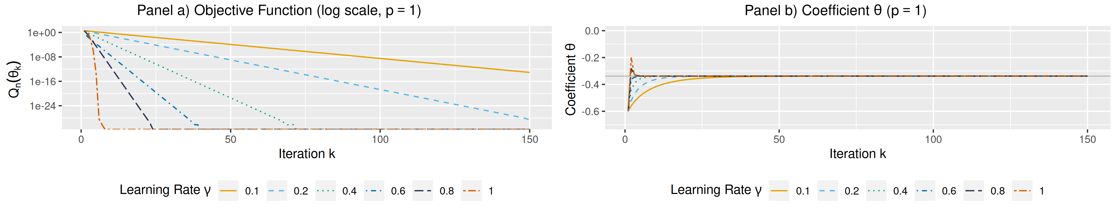
Figure C7: gn iterations: different learning rates

Legend: simulated sample of size $n=200$, $\theta^{\dagger}=-1/2$, $\overline{g}_{n}(\theta)=\hat{\beta}_{n}-\beta(\theta)$. Grey horizontal line: $\hat{\theta}_{n}=-0.339$. Just Identified ($p=1$).

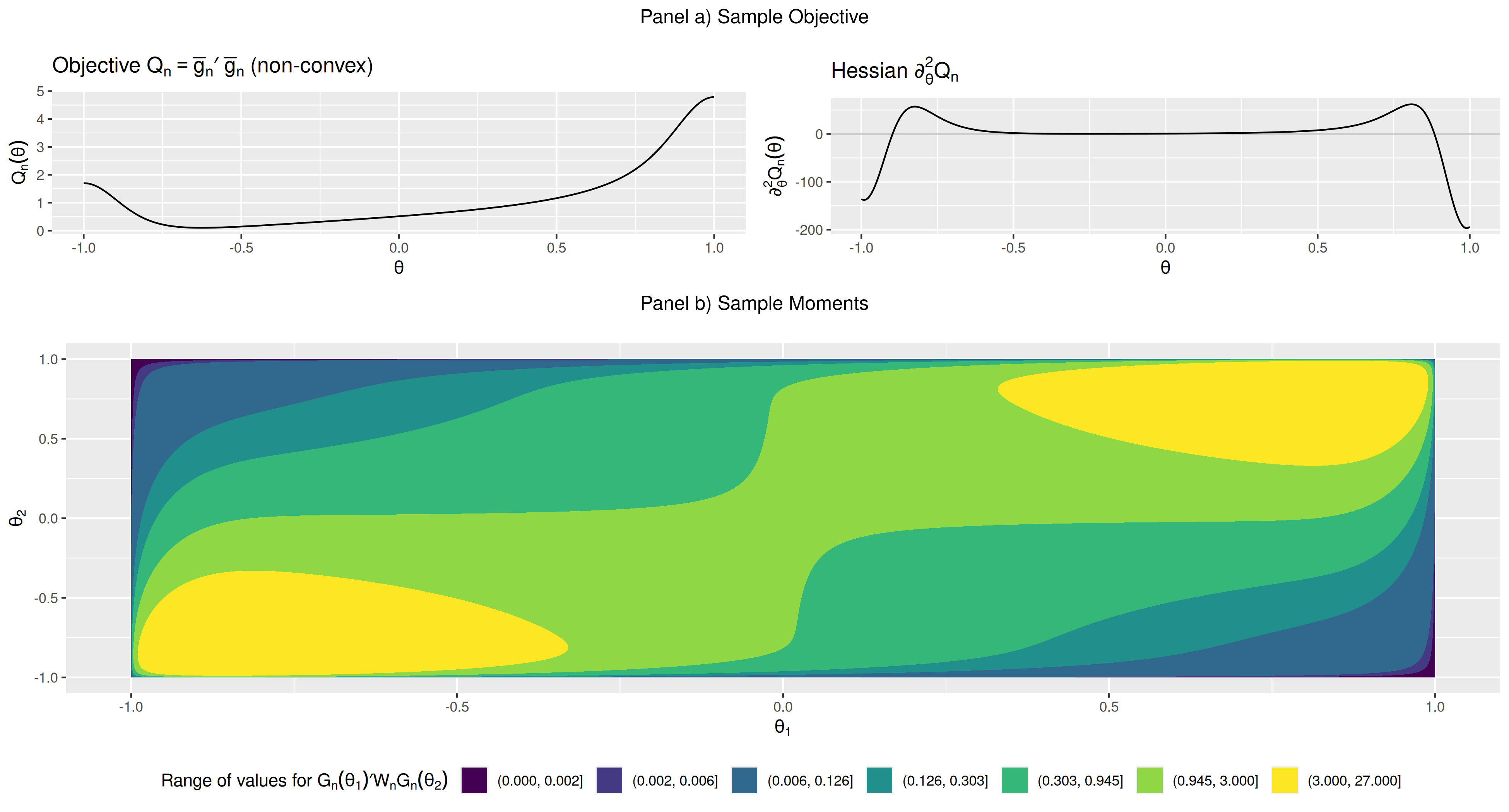
Figure C8: Non-convexity and the rank condition ($p=12$, equal weighting $W_{n}=I_{d}$)

Legend: simulated sample of size $n=200$, $\theta^{\dagger}=-1/2$, $\overline{g}_{n}(\theta)=\hat{\beta}_{n}-\beta(\theta)$, $W_{n}=I_{d}$. The GMM objective (panel a) is non-convex but the sample moments (panel b) satisfy the rank condition: $G_{n}(\theta_{1})^{\prime}G_{n}(\theta_{2})$ is full rank (non-zero) for all $(\theta_{1},\theta_{2})\in(-1,1)\times(-1,1)$.

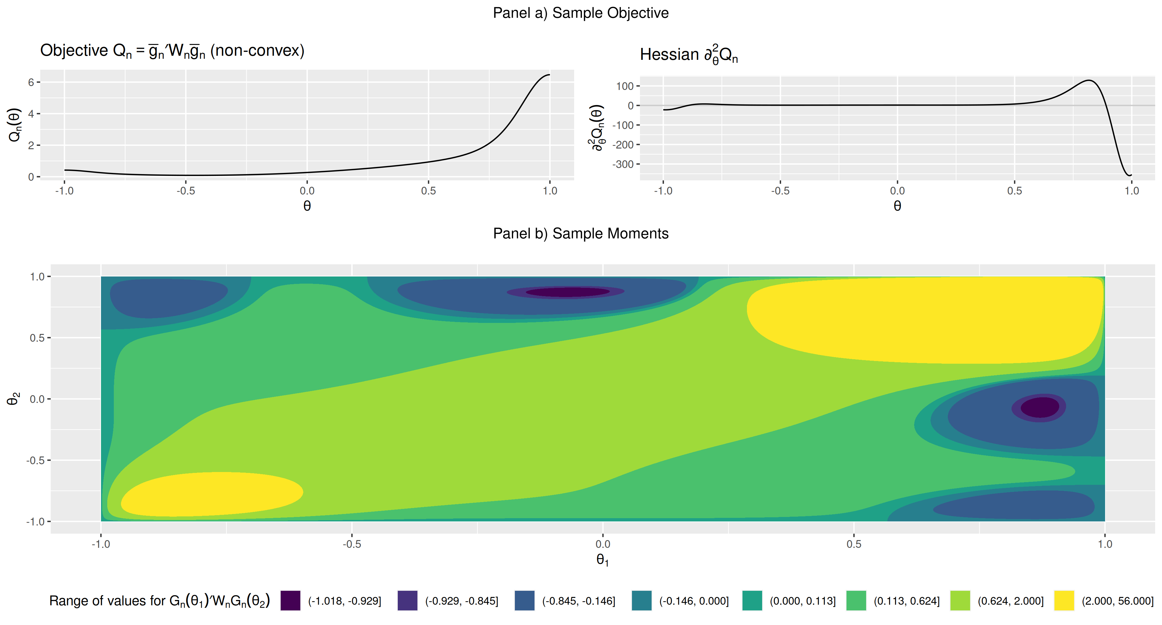
Figure C9: Non-convexity and the rank condition ($p=12$, optimal weighting $W_{n}=V_{n}^{-1}$)

Legend: simulated sample of size $n=200$, $\theta^{\dagger}=-1/2$, $\overline{g}_{n}(\theta)=\hat{\beta}_{n}-\beta(\theta)$, $W_{n}=V_{n}^{-1}$ with $V_{n}=n\hat{\text{var}}(\hat{\beta}_{n})$. The GMM objective (panel a) is non-convex but the sample moments (panel b) does not satisfy the rank condition: $G_{n}(\theta_{1})^{\prime}V_{n}^{-1}G_{n}(\theta_{2})$ is not full rank (non-zero) for all $(\theta_{1},\theta_{2})\in(-1,1)\times(-1,1)$.

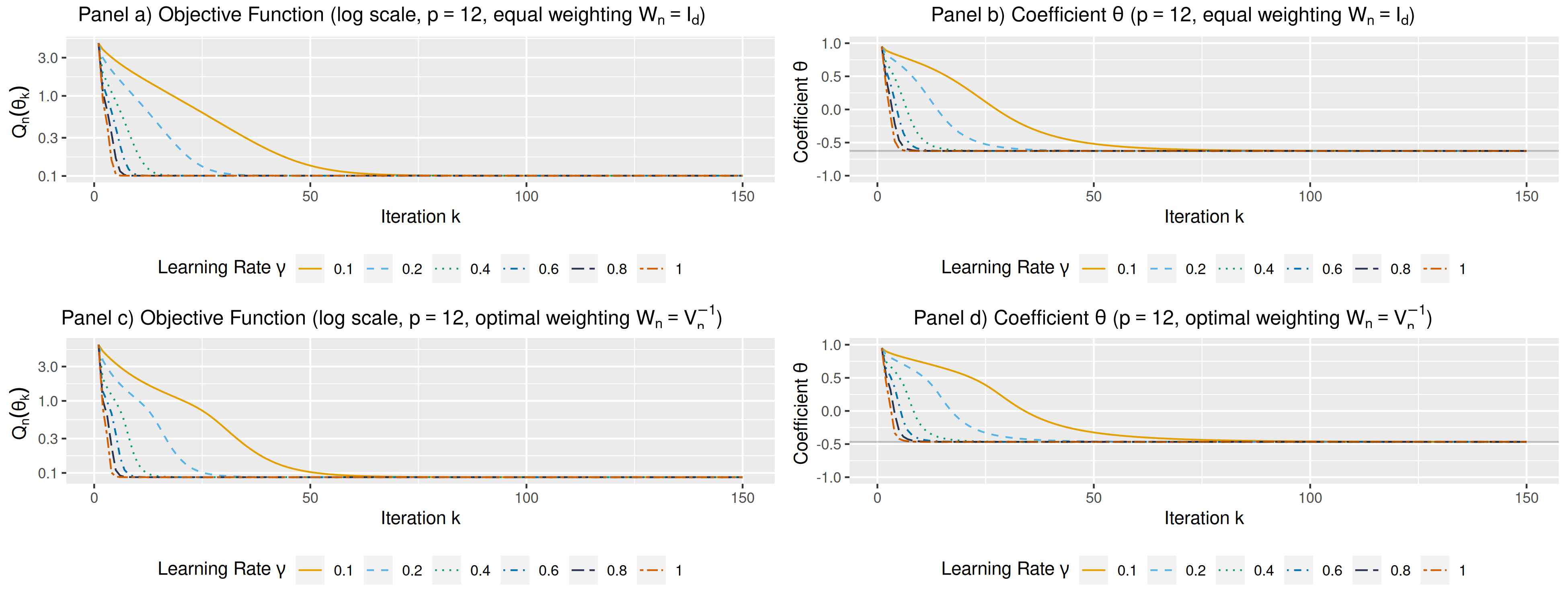
Figure C10: gn iterations: equal and optimal weighting, different learning rates

Legend: simulated sample of size $n=200$, $\theta^{\dagger}=-1/2$, $\overline{g}_{n}(\theta)=\hat{\beta}_{n}-\beta(\theta)$, $W_{n}=I_{d}$ (equal weighting, top panel), or $W_{n}=V_{n}^{-1}$ (optimal weighting, bottom panel), with $V_{n}=n\hat{\text{var}}(\hat{\beta}_{n})$. Grey horizontal line: $\hat{\theta}_{n}=-0.626$ (equal weighting), $\hat{\theta}_{n}=-0.466$ (optimal weighting).

C.2 Demand for Cereal

Table C5: Demand for Cereal: gn with different learning rates

		stdev				income				objs	# of
		const.	price	sugar	mushy	const.	price	sugar	mushy		crashes
true	est	0.28	2.03	-0.01	-0.08	3.58	0.47	-0.17	0.69	33.84	-
	se	0.11	0.76	0.01	0.15	0.56	3.06	0.02	0.26	-
	avg	0.28	2.03	-0.01	-0.08	3.58	0.47	-0.17	0.69	33.84
$\gamma=0.1$	std	0.00	0.00	0.00	0.00	0.00	0.00	0.00	0.00	0.00	0
	avg	0.28	2.03	-0.01	-0.08	3.58	0.47	-0.17	0.69	33.84
$\gamma=0.2$	std	0.00	0.00	0.00	0.00	0.00	0.00	0.00	0.00	0.00	0
	avg	0.28	2.03	-0.01	-0.08	3.58	0.47	-0.17	0.69	33.84
$\gamma=0.4$	std	0.00	0.00	0.00	0.00	0.00	0.00	0.00	0.00	0.00	0
	avg	0.28	2.03	-0.01	-0.08	3.58	0.47	-0.17	0.69	33.84
$\gamma=0.6$	std	0.00	0.00	0.00	0.00	0.00	0.00	0.00	0.00	0.00	0
	avg	0.28	2.03	-0.01	-0.08	3.58	0.47	-0.17	0.69	33.84
$\gamma=0.8$	std	0.00	0.00	0.00	0.00	0.00	0.00	0.00	0.00	0.00	0
	avg	0.28	2.03	-0.01	-0.08	3.58	0.47	-0.17	0.69	33.84
$\gamma=1$	std	0.00	0.00	0.00	0.00	0.00	0.00	0.00	0.00	0.00	0

Legend: Comparison for 50 starting values in $[-10,10]\times\dots\times[-10,10]$. Avg, Std: sample average and standard deviation of optimizer outputs. true: full sample estimate (est) and standard errors (se). Objs: avg and std of minimized objective value. # of crashes: optimization terminated because the objective function returned an error. gn run with $\gamma\in\{0.1,0.2,0.4,0.6,0.8,1\}$ for $k=150$ iterations for all starting values.

C.3 Impulse Response Matching

The following tables report results for gn using a range of tuning parameters $\gamma$. Since the rank condition (3’) does not hold towards the lower bound for $\eta,\nu$, gn alone can crash and/or fail to converge. Following Forneron (2023), we can introduce a global step:

$$\theta_{k+1}=\theta_{k}-\gamma P_{k}G_{n}(\theta_{k})^{\prime}W_{n}\overline{g}_{n}(\theta_{k})$$ (1)

$$\text{if }\|\overline{g}_{n}(\theta^{k+1})\|_{W_{n}}<\|\overline{g}_{n}(\theta_{k+1})\|_{W_{n}},\text{ set }\theta_{k+1}=\theta^{k+1}$$

where the sequence $(\theta^{k})_{k\geq 0}$ is predetermined and dense in $\Theta$. The results rely on the Sobol sequence, independently randomized for each of the 50 starting values. Results are reported with and without the global step. Also, the former implements error-handling (try-catch).

Table C6: Without reparameterization : gn with different learning rates

		$\eta$	$\nu$	$\rho_{s}$	$\sigma_{s}$	objs	# of crashes
true	est	0.30	0.29	0.39	0.17	4.65	-
gn without global step
	avg	0.30	0.29	0.39	0.17	4.65
$\gamma=0.1$	std	0.00	0.00	0.00	0.00	0.00	2
	avg	0.30	0.29	0.39	0.17	4.65
$\gamma=0.2$	std	0.00	0.00	0.00	0.00	0.00	2
	avg	0.30	0.29	0.39	0.17	4.65
$\gamma=0.4$	std	0.00	0.00	0.00	0.00	0.00	4
	avg	0.30	0.29	0.39	0.17	4.65
$\gamma=0.6$	std	0.00	0.00	0.00	0.00	0.00	8
	avg	0.30	0.29	0.39	0.17	4.65
$\gamma=0.8$	std	0.00	0.00	0.00	0.00	0.00	12
	avg	0.30	0.29	0.39	0.17	4.65
$\gamma=1$	std	0.00	0.00	0.00	0.00	0.00	28
gn with global step
	avg	0.30	0.29	0.39	0.17	4.65
$\gamma=0.1$	std	0.00	0.00	0.00	0.00	0.00	0
	avg	0.30	0.29	0.39	0.17	4.65
$\gamma=0.2$	std	0.00	0.00	0.00	0.00	0.00	0
	avg	0.30	0.29	0.39	0.17	4.65
$\gamma=0.4$	std	0.00	0.00	0.00	0.00	0.00	0
	avg	0.30	0.29	0.39	0.17	4.65
$\gamma=0.6$	std	0.00	0.00	0.00	0.00	0.00	0
	avg	0.30	0.29	0.39	0.17	4.65
$\gamma=0.8$	std	0.00	0.00	0.00	0.00	0.00	0
	avg	0.30	0.29	0.39	0.17	4.65
$\gamma=1$	std	0.00	0.00	0.00	0.00	0.00	0
lower bound		0.05	0.01	-0.95	0.01	-	-
upper bound		0.99	0.90	0.95	12	-	-

Legend: Comparison for 50 starting values. true: full sample estimate (est). gn with global step: Gauss-Netwon augmented with a global sequence. Both are run for $k=150$ iterations in total, for all starting values. Objs: avg and std of minimized objective value. # of crashes: optimization terminated because objective returned error. Lower/upper bound used for the reparameterization.

Table C7: With reparameterization : gn with different learning rates

		$\eta$	$\nu$	$\rho_{s}$	$\sigma_{s}$	objs	# of crashes
true	est	0.30	0.29	0.39	0.17	4.65	-
gn without global step
	avg	0.30	0.29	0.39	0.17	4.65
$\gamma=0.1$	std	0.00	0.00	0.00	0.00	0.00	5
	avg	0.30	0.29	0.39	0.17	4.65
$\gamma=0.2$	std	0.00	0.00	0.00	0.00	0.00	10
	avg	0.30	0.29	0.39	0.17	4.65
$\gamma=0.4$	std	0.00	0.00	0.00	0.00	0.00	20
	avg	0.30	0.29	0.39	0.17	4.65
$\gamma=0.6$	std	0.00	0.00	0.00	0.00	0.00	22
	avg	0.30	0.29	0.39	0.17	4.65
$\gamma=0.8$	std	0.00	0.00	0.00	0.00	0.00	25
	avg	0.30	0.29	0.39	0.17	4.65
$\gamma=1$	std	0.00	0.00	0.00	0.00	0.00	29
gn with global step
	avg	0.30	0.29	0.39	0.17	4.65
$\gamma=0.1$	std	0.00	0.00	0.00	0.00	0.00	0
	avg	0.30	0.29	0.39	0.17	4.65
$\gamma=0.2$	std	0.00	0.00	0.00	0.00	0.00	0
	avg	0.30	0.29	0.39	0.17	4.65
$\gamma=0.4$	std	0.00	0.00	0.00	0.00	0.00	0
	avg	0.30	0.29	0.39	0.17	4.65
$\gamma=0.6$	std	0.00	0.00	0.00	0.00	0.00	0
	avg	0.30	0.29	0.39	0.17	4.65
$\gamma=0.8$	std	0.00	0.00	0.00	0.00	0.00	0
	avg	0.30	0.29	0.39	0.17	4.65
$\gamma=1$	std	0.00	0.00	0.00	0.00	0.00	0
lower bound		0.05	0.01	-0.95	0.01	-	-
upper bound		0.99	0.90	0.95	12	-	-

Legend: Comparison for 50 starting values. true: full sample estimate (est). gn with global step: Gauss-Netwon augmented with a global sequence. Both are run for $k=150$ iterations in total, for all starting values. Objs: avg and std of minimized objective value. # of crashes: optimization terminated because objective returned error. Lower/upper bound used for the reparameterization.

Appendix D Additional Material for Section 2.2

The Nelder-Mead algorithm.

The following description of the algorithm is based on Nash (1990, Ch14) which R implements in the optimizer optim. The first step is to build a simplex for the $p$-dimensional parameters, i.e. $p+1$ distinct points $\theta_{1},\dots,\theta_{p+1}$ ordered s.t. $Q_{n}(\theta_{1})\leq\dots\leq Q_{n}(\theta_{p+1})$. The simplex is then transformed at each iteration using four operations called reflection, expansion, reduction, and contraction. The algorithm also repeatedly computes the centroid $\theta_{c}$ of the best $p$ points, to do so: take the best $p$ guesses $\theta_{1},\dots,\theta_{p}$ and compute their average: $\theta_{c}=1/p\sum_{\ell=1}^{p}\theta_{\ell}$. Once this is done, go to step R below.

Clearly, the choice of initial simplex can affect the convergence of the algorithm. Typically, one provides a starting value $\theta_{1}$ and then the software picks the remaining $p$ points of the simplex without user input. NM proposed their algorithm with statistical estimation in mind, so they considered using the standard deviation $\sqrt{\sum_{\ell=1}^{n+1}(Q_{n}(\theta_{\ell})-\bar{Q}_{n})^{2}/n}<\text{tol}$ as a convergence criterion, setting $\text{tol}=10^{-8}$ and $\bar{Q}_{n}$ the average of $Q_{n}(\theta_{\ell})$ in their application. Here convergence occurs when the simplex collapses around a single point.

The Grid-Search algorithm.

The procedure is very simple, pick a grid of $k$ points $\theta_{1},\dots,\theta_{k}$, and compute:

$$\tilde{\theta}_{k}=\text{argmin}_{\ell=1,\dots,k}Q_{n}(\theta_{\ell}).$$

The optimization error $\|\tilde{\theta}_{k}-\hat{\theta}_{n}\|$ depends on both $k$ and the choice of grid. The following gives an overview of the approximation error and feasible error rates.

For simplicity, suppose that the parameter space is the unit ball in $\mathbb{R}^{p}$: $\Theta=\mathcal{B}_{2}^{p}$, and $Q_{n}$ is continuous. Under these assumptions, there is an $L\geq 0$ such that $|Q_{n}(\theta_{1})-Q_{n}(\theta_{2})|\leq L\|\theta_{1}-\theta_{2}\|$. $L>0$, unless $Q_{n}$ is constant. This implies: $|Q_{n}(\tilde{\theta}_{k})-Q_{n}(\hat{\theta}_{n})|\leq L(\inf_{1\leq\ell\leq k}\|\theta_{\ell}-\hat{\theta}_{n}\|)$. Suppose we want to ensure $|Q_{n}(\tilde{\theta}_{k})-Q_{n}(\hat{\theta}_{n})|\leq\varepsilon$, then we need $\inf_{1\leq\ell\leq k}\|\theta_{\ell}-\hat{\theta}_{n}\|\leq\varepsilon/L$. Packing arguments (e.g. Vershynin, 2018, Proposition 4.2.12) give a lower bound for $k$ over all grids, and all possible $\hat{\theta}_{n}$: $k\geq\text{vol}(\mathcal{B}_{2}^{p})/\text{vol}([\varepsilon/L]\mathcal{B}_{2}^{p})=[\varepsilon/L]^{-p}$, where vol is the volume.

For the choice of grid, Niederreiter (1983, Theorem 3) shows that low-discrepancy sequences, e.g. the Sobol or Halton points sets, can achieve this rate, up to a logarithmic term. This is indeed a common choice for multi-start and grid search optimization.

In practice, $Q_{n}(\tilde{\theta}_{k})-Q_{n}(\hat{\theta}_{n})$ is typically not the quantity of interest for empirical estimations, rather we are interested in $\|\tilde{\theta}_{k}-\hat{\theta}_{n}\|$. Suppose, in addition, that $\hat{\theta}_{n}\in\text{int}(\Theta)$, and $Q_{n}$ is twice continuously differentiable with positive definite Hessian $H_{n}(\hat{\theta}_{n})$, a local identification condition. Then there exists $0<\underline{\lambda}\leq\overline{\lambda}<\infty$ and $\varepsilon_{1}>0$ s.t. $\|\theta-\hat{\theta}_{n}\|\leq\varepsilon_{1}$ implies:

$$\underline{\lambda}\|\theta-\hat{\theta}_{n}\|^{2}\leq Q_{n}(\theta)-Q_{n}(\hat{\theta}_{n})\leq\overline{\lambda}\|\theta-\hat{\theta}_{n}\|^{2},$$ (D.10)

i.e. $Q_{n}$ is locally strictly convex. If $\hat{\theta}_{n}$ is the unique minimizer of $Q_{n}$, there is a $0<\varepsilon_{2}\leq\varepsilon_{1}$ such that $\inf_{\|\theta-\hat{\theta}_{n}\|\geq\varepsilon_{1}}Q_{n}(\theta)>Q_{n}(\hat{\theta}_{n})+\overline{\lambda}\varepsilon_{2}^{2}$, using a global identification condition. Now, by local identification: $\|\theta-\hat{\theta}_{n}\|\leq\varepsilon_{2}\Rightarrow Q_{n}(\theta)\leq Q_{n}(\hat{\theta}_{n})+\overline{\lambda}\varepsilon_{2}^{2}<\inf_{\|\theta-\hat{\theta}_{n}\|\geq\varepsilon_{1}}Q_{n}(\theta)$. As soon as $k\geq k_{0}$ where $\inf_{1\leq\ell\leq k_{0}}\|\theta_{\ell}-\hat{\theta}_{n}\|\leq\varepsilon_{2}$, we have $\|\tilde{\theta}_{k}-\hat{\theta}_{n}\|\leq\varepsilon_{1}$. Then, for any $k\geq k_{0}$: $\underline{\lambda}\|\tilde{\theta}_{k}-\hat{\theta}_{n}\|^{2}\leq Q_{n}(\tilde{\theta}_{k})-Q_{n}(\hat{\theta}_{n})\leq\overline{\lambda}(\inf_{1\leq\ell\leq k}\|\theta_{\ell}-\hat{\theta}_{n}\|^{2})$ and $\|\tilde{\theta}_{k}-\hat{\theta}_{n}\|\leq[\overline{\lambda}/\underline{\lambda}]^{1/2}(\inf_{1\leq\ell\leq k}\|\theta_{\ell}-\hat{\theta}_{n}\|).$

This reveals the interplay between the identification conditions and the optimization error. The best value $\tilde{\theta}_{k}$ is only guaranteed to be near $\hat{\theta}_{n}$ when $k\geq\varepsilon_{2}^{-p}$ iterations (using packing arguments for the unit ball), where $\varepsilon_{2}$ depends on the global identification condition. Local convergence depends on the ratio $\overline{\lambda}/\underline{\lambda}\geq 1$ which is infinite when $H_{n}(\hat{\theta}_{n})$ is singular. The main drawback of a grid search is its slow convergence. To illustrate, Colacito et al. (2018, pp3443-3445) estimate $p=5$ parameters using a grid search with $k=1551$ points. For simplicity, suppose $\overline{\lambda}/\underline{\lambda}=1$, $k_{0}<k$, and $\Theta=\mathcal{B}_{2}^{p}$, the unit ball, then the worst-case optimization error is $\sup_{\hat{\theta}_{n}\in\Theta}(\inf_{1\leq\ell\leq k}\|\theta_{\ell}-\hat{\theta}_{n}\|)\geq k^{-1/p}\simeq 0.23$. This is ten times larger than all but one of the standard errors reported in the paper.

Simulated Annealing.

Implementations can vary across software, the following will focus on the implementation used in R’s optim function.

The implementation described above relies on the random-walk Metropolis update. Notice that if $Q_{n}(\theta^{\star})\leq Q_{n}(\theta_{\ell-1})$, the exponential term in step 2 is greater than $1$ and $\theta^{\star}$ is always accepted as the next $\theta_{\ell}$, regardless of $u_{\ell}$. Bélisle (1992) gave sufficient condition for $\tilde{\theta}_{k}\overset{a.s.}{\to}\hat{\theta}_{n}$ when $k\to\infty$ and $Q_{n}$ is continuous. In practice, the performance of the Algorithm can be measured by its convergence rate. To get some intuition, we give some simplified derivations below which highlight the role of $T_{k}$ and several quantities which appeared in our discussion of the grid search.

First, notice that for each $k$, steps 1-2 implement the Metropolis algorithm also used for Bayesian inference using random-walk Metropolis-Hastings. The invariant distribution of these two steps is:

$$f_{k}(\theta)=\frac{\exp(-[Q_{n}(\theta)-Q_{n}(\hat{\theta}_{n})]/T_{k})}{\int_{\Theta}\exp(-[Q_{n}(\theta)-Q_{n}(\hat{\theta}_{n})]/T_{k})d\theta},$$

this is called the Gibbs-Boltzmann distribution. When $T_{\infty}=+\infty$, $f_{\infty}$ puts all the probability mass on the unique minimum $\hat{\theta}_{n}$. To build intuition, suppose that $k\geq 1$: $\theta_{k}\sim f_{k}$. Because SA is a stochastic algorithm, the approximation error $\|\theta_{k}-\hat{\theta}_{n}\|$ is random, but can be quantified using $\mathbb{P}(\|\theta_{k}-\hat{\theta}_{n}\|\geq\varepsilon)$. In the following we will assume the temperature schedule to be $T_{k}=T_{1}/\log(k)$, as implemented in R.

The following relies on the same setting, notation and assumptions as the grid search above. First, we can bound the probability that $\theta_{k}$ is outside the $\varepsilon_{1}$-local neighborhood of $\hat{\theta}_{n}$ where $Q_{n}$ is approximately quadratic: $\mathbb{P}(\|\theta_{k}-\hat{\theta}_{n}\|\geq\varepsilon_{1})$. Using the global identification condition:

$$\exp(-[Q_{n}(\theta)-Q_{n}(\hat{\theta}_{n})]/T_{k})\leq\exp(-\overline{\lambda}\varepsilon_{2}^{2}/T_{k})=k^{-\overline{\lambda}\varepsilon_{2}^{2}/T_{1}},\text{ if }\|\theta-\hat{\theta}_{n}\|\geq\varepsilon_{1},$$

where $\varepsilon_{1},$ $\varepsilon_{2}$ were defined in the grid search section above. This gives an upper bound for the numerator in $f_{k}(\theta_{k})$. A lower bound is also required for the denominator. Using (D.10) and the change of variable $\theta=\hat{\theta}_{n}+\sqrt{T_{k}}h$, we have:

$$\exp(-\overline{\lambda}\|h\|^{2})\leq\exp(-[Q_{n}(\hat{\theta}_{n}+\sqrt{T_{k}}h)-Q_{n}(\hat{\theta}_{n})]/T_{k})\leq\exp(-\underline{\lambda}\|h\|^{2}),\text{ if }\|\sqrt{T_{k}}h\|\leq\varepsilon_{1}.$$

Suppose $T_{k}\leq\varepsilon_{1}^{2}$, the two inequalities give us the bound:

$$\mathbb{P}(\|\theta_{k}-\hat{\theta}_{n}\|\geq\varepsilon_{1})\leq\frac{k^{-\overline{\lambda}\varepsilon_{2}^{2}/T_{1}}\text{vol}(\Theta)}{|T_{k}|^{p/2}\int_{\|h\|\leq 1}\exp(-\overline{\lambda}\|h\|^{2})dh}=C[\log(k)]^{d/2}k^{-\overline{\lambda}\varepsilon_{2}^{2}/T_{1}}.$$

This upper bound declines more slowly than for the grid search when $\overline{\lambda}\varepsilon_{2}^{2}/T_{1}<1/p$, which can be the case if $T_{1}$ large and/or $\varepsilon_{2}$ is small. For the lower bound, pick any $\varepsilon\in(0,\varepsilon_{1}/\sqrt{T_{k}})$:

$$\mathbb{P}(\|\theta_{k}-\hat{\theta}_{n}\|\leq\sqrt{T_{k}}\varepsilon)\geq\frac{\int_{\|h\|\leq\varepsilon}\exp(-\overline{\lambda}\|h\|^{2})dh}{\int_{\|h\|\in\mathbb{R}}\exp(-\underline{\lambda}\|h\|^{2})dh+|T_{k}|^{-p/2}\text{vol}(\Theta)k^{-\overline{\lambda}\varepsilon_{2}^{2}/T_{1}}},$$

which has a strictly positive limit. This implies that $\sqrt{\log(k)}\|\theta_{k}-\hat{\theta}_{n}\|\geq O_{p}(1)$, since $T_{k}=T_{1}/\log(k)$. This $\sqrt{\log(k)}$ rate is slower than the grid search. To get faster convergence, some authors have suggested using $T_{k}=T_{1}/k$ and, by default, Matlab sets $T_{k}=T_{1}\cdot 0.95^{k}$. However, theoretical guarantees to have $\theta_{k}\overset{p}{\to}\hat{\theta}_{n}$, as $k\to\infty$ are only available when $T_{k}=T_{1}/\log(k)$.

References

- Andrews (1997) Andrews, D. W. (1997): “A stopping rule for the computation of generalized method of moments estimators,” Econometrica: Journal of the Econometric Society, 913–931.
- Arnoud et al. (2019) Arnoud, A., F. Guvenen, and T. Kleineberg (2019): “Benchmarking Global Optimizers,” NBER Working Paper.
- Bélisle (1992) Bélisle, C. J. (1992): “Convergence theorems for a class of simulated annealing algorithms on ,” Journal of Applied Probability, 29, 885–895.
- Berry et al. (1995) Berry, S., J. Levinsohn, and A. Pakes (1995): “Automobile Prices in Market Equilibrium,” Econometrica, 63, 841.
- Bhatia (2013) Bhatia, R. (2013): Matrix Analysis, vol. 169, Springer Science & Business Media.
- Brunner et al. (2017) Brunner, D., F. Heiss, A. Romahn, and C. Weiser (2017): Reliable estimation of random coefficient logit demand models, 267, DICE Discussion Paper.
- Cameron and Trivedi (2005) Cameron, A. C. and P. K. Trivedi (2005): Microeconometrics: methods and applications, Cambridge University Press.
- Chernozhukov and Hong (2003) Chernozhukov, V. and H. Hong (2003): “An MCMC approach to classical estimation,” Journal of Econometrics, 115, 293–346.
- Colacito et al. (2018) Colacito, R., M. Croce, S. Ho, and P. Howard (2018): “BKK the EZ way: International long-run growth news and capital flows,” American Economic Review, 108, 3416–49.
- Conlon and Gortmaker (2020) Conlon, C. and J. Gortmaker (2020): “Best practices for differentiated products demand estimation with pyblp,” The RAND Journal of Economics, 51, 1108–1161.
- Davidson et al. (2004) Davidson, R., J. G. MacKinnon, et al. (2004): Econometric theory and methods, vol. 5, Oxford University Press New York.
- Dennis and Schnabel (1996) Dennis, J. E. and R. B. Schnabel (1996): Numerical methods for unconstrained optimization and nonlinear equations, SIAM.
- Deuflhard (2005) Deuflhard, P. (2005): Newton methods for nonlinear problems: affine invariance and adaptive algorithms, vol. 35, Springer Science & Business Media.
- Donaldson (2018) Donaldson, D. (2018): “Railroads of the Raj: Estimating the impact of transportation infrastructure,” American Economic Review, 108, 899–934.
- Fang and Wang (1993) Fang, K.-T. and Y. Wang (1993): Number-theoretic methods in statistics, vol. 51, CRC Press.
- Forneron (2023) Forneron, J.-J. (2023): “Noisy, Non-Smooth, Non-Convex Estimation of Moment Condition Models,” arXiv preprint arXiv:2301.07196.
- Gourieroux and Monfort (1996) Gourieroux, C. and A. Monfort (1996): Simulation-based econometric methods, Oxford university press.
- Hall and Inoue (2003) Hall, A. R. and A. Inoue (2003): “The large sample behaviour of the generalized method of moments estimator in misspecified models,” Journal of Econometrics, 114, 361–394.
- Hansen (2022a) Hansen, B. E. (2022a): Econometrics, Princeton University Press.
- Hansen (2022b) ——— (2022b): Probability and Statistics for Economists, Princeton University Press.
- Hansen and Lee (2021) Hansen, B. E. and S. Lee (2021): “Inference for iterated GMM under misspecification,” Econometrica, 89, 1419–1447.
- Hayashi (2011) Hayashi, F. (2011): Econometrics, Princeton University Press.
- Jennrich (1969) Jennrich, R. I. (1969): “Asymptotic properties of non-linear least squares estimators,” The Annals of Mathematical Statistics, 40, 633–643.
- Knittel and Metaxoglou (2014) Knittel, C. R. and K. Metaxoglou (2014): “Estimation of random-coefficient demand models: two empiricists’ perspective,” Review of Economics and Statistics, 96, 34–59.
- Lagarias et al. (1998) Lagarias, J. C., J. A. Reeds, M. H. Wright, and P. E. Wright (1998): “Convergence properties of the Nelder–Mead simplex method in low dimensions,” SIAM Journal on optimization, 9, 112–147.
- Lemieux (2009) Lemieux, C. (2009): Monte Carlo and Quasi-Monte Carlo Sampling, Springer Series in Statistics, Springer New York.
- Lise and Robin (2017) Lise, J. and J.-M. Robin (2017): “The Macrodynamics of Sorting between Workers and Firms,” American Economic Review, 107, 1104–35.
- McCullough and Vinod (2003) McCullough, B. D. and H. D. Vinod (2003): “Verifying the solution from a nonlinear solver: A case study,” American Economic Review, 93, 873–892.
- McKinnon (1998) McKinnon, K. I. (1998): “Convergence of the Nelder–Mead Simplex method to a nonstationary Point,” SIAM Journal on optimization, 9, 148–158.
- Moran and Queralto (2018) Moran, P. and A. Queralto (2018): “Innovation, productivity, and monetary policy,” Journal of Monetary Economics, 93, 24–41.
- Nash (1990) Nash, J. C. (1990): Compact numerical methods for computers: linear algebra and function minimisation, Routledge.
- Nelder and Mead (1965) Nelder, J. A. and R. Mead (1965): “A simplex method for function minimization,” The computer journal, 7, 308–313.
- Nevo (2001) Nevo, A. (2001): “Measuring market power in the ready-to-eat cereal industry,” Econometrica, 69, 307–342.
- Newey and McFadden (1994) Newey, W. and D. McFadden (1994): “Large Sample Estimation and Hypothesis Testing,” in Handbook of Econometrics, North Holland, vol. 36:4, 2111–2234.
- Niederreiter (1983) Niederreiter, H. (1983): “A quasi-Monte Carlo method for the approximate computation of the extreme values of a function,” in Studies in pure mathematics, Springer, 523–529.
- Nocedal and Wright (2006) Nocedal, J. and S. Wright (2006): Numerical Optimzation, Springer, second ed.
- Powell (1973) Powell, M. J. (1973): “On search directions for minimization algorithms,” Mathematical programming, 4, 193–201.
- Quandt (1983) Quandt, R. E. (1983): “Computational problems and methods,” Handbook of econometrics, 1, 699–764.
- Rothenberg (1971) Rothenberg, T. J. (1971): “Identification in parametric models,” Econometrica: Journal of the Econometric Society, 577–591.
- Salanié and Wolak (2022) Salanié, B. and F. A. Wolak (2022): “Fast, Detail-free, and Approximately Correct: Estimating Mixed Demand Systems,” .
- Spall (2005) Spall, J. C. (2005): Introduction to stochastic search and optimization: estimation, simulation, and control, John Wiley & Sons.
- Stokes (2004) Stokes, H. H. (2004): “On the advantage of using two or more econometric software systems to solve the same problem,” Journal of Economic and Social Measurement, 29, 307–320.
- Vershynin (2018) Vershynin, R. (2018): High-dimensional probability: An introduction with applications in data science, vol. 47, Cambridge university press.
- Wooldridge (2010) Wooldridge, J. M. (2010): Econometric analysis of cross section and panel data, MIT press.