ganX - generate artificially new XRF
a python library to generate MA-XRF raw data out of RGB images

Abstract

In this paper we present the first version of ganX - generate artificially new XRF, a Python library to generate X-ray fluorescence Macro maps (MA-XRF) from a coloured RGB image. To do that, a Monte Carlo method is used, where each MA-XRF pixel signal is sampled out of an XRF signal probability function. Such probability function is computed using a database of couples (pigment characteristic XRF signal, RGB), by a weighted sum of such pigment XRF signal by proximity of the image RGB to the pigment characteristic RGB. The library is released to PyPi and the code is available open source on GitHub.

Keywords Python  $\cdot$ Synthetic Dataset generation  $\cdot$ X-ray Fluorescence Macro mapping (MA-XRF)  $\cdot$ Cultural Heritage,  $\cdot$ Monte Carlo methods  $\cdot$ Artificial Intelligence, Statistical and Deep Learning

1 Introduction

In the last decade, we have witnessed a truly remarkable rise of Artificial Intelligence, Statistical and Deep learning methods (for a non exhaustive list of papers on the history of deep learning, see [1, 2, 3], and references therein).

Inspired by the incredible results obtained thanks to the application of such methods to scientific problems, its adoption in the field of nuclear imaging applied to Cultural Heritage (CH) has begun (see, e.g., [4, 5, 6, 7, 8], especially the nice overview [9], and, of course, the references therein), also in the field of X-ray fluorescence Macro mapping (MA-XRF) [10, 11, 12, 13, 14, 15]. In MA-XRF, the imaging apparatus produces a data cube which, for each pixel, is formed by a spectrum containing fluorescence lines associated with the element composition of the pigment present in the pictorial layers.

MA-XRF data cubes offer an ideal framework for application of unsupervised statistical learning methods [13], due to the huge number of pixel XRF histogram w.r.t. the relatively small number of employed pigment palettes.

Unfortunately, in the realm of supervised statistical (deep) learning applied to CH-based analysis, the situation is flipped [14], since the data cube production is slow, obtaining a small dataset for the complexity of the various task at hand (like automatic pigment identification [14, 15], element recognition [16], and even colour association [11, 12]).

This justifies the emphasis put on the creation of ad hoc synthetic MA-XRF dataset [14]. In this brief paper, we present ganX [17], a Python library for creating synthetic dataset of MA-XRF images, starting from

1. A (set of) RGB image(s); and

2. A Database of pigments;

Such database must have

• A characteristic XRF signal;

• A characteristic, 8-bit, RGB colour.

ganX will use (b) to associate pigment(s) to RGB pixels, and (a) as a probability distribution to generate the MA-XRF data cube via Monte Carlo methods.

At the day of writing, the package is available open access on the Python Package index (PyPi). The package code is open source on GitHub [17], where its documentation is available.

2 Main idea

Inspired by the work done in [14], where the authors generate a synthetic dataset of single-point XRF histogram by using the Fundamental Parameters (FP) method, a physical model based on Sherman’s equations for generating XRF spectra of a sample of known composition [18], we started the development of a simple python package capable of creating MA-XRF data cubes starting from a RGB image and a database of pigments’ XRF signal.

The data generation algorithm comprises two main parts:

1. A RGB clustering of the input image(s), performed with an iterative K-Means, to reduce the colour noise;

2. A Monte Carlo method to generate a XRF histogram of counts for each pixel, after having unsupervisedly associated a (set of) pigment(s) to each RGB pixel.

To perform step 2. above, we compute (pixel-by-pixel) a set of similarity measures in RGB spaces, between the (clustered) RGB and the database indexed pigments’ characteristic RGB; then, an hard thresholding is performed, to (unsupervisedly) reduce the number of pigments.

The full pseudocode of the MA-XRF data generation is

Algorithm 1 Generate MA-XRF

1:RGBclustering, distrToXrf, colorSimilarity $\triangleright$ Import relevant methods

2:procedure generateXRF(pigments_dict_data = $\mathcal{D}_{{color},{hist}}$, rgb_img = $R$)

3:     $R\leftarrow$ RGBclustering($R$)

4:     init $X$; $\triangleright$ Initialise empy XRF data cube

5:     for $r\in R$ do $\triangleright$ Iterate over clusters

6:         init $d$; $\triangleright$ Initialise empty distribution

7:         for $(c,h)\in\mathcal{D}$ do $\triangleright$ Iterate over database

8:              $\alpha\leftarrow$ colorSimilarity($c,r$)

9:              if $\alpha\geq\alpha_{th}$ then

10:                  $d\leftarrow d+\alpha\cdot h$ $\triangleright$ Sum thresholded distribution                        

11:         $d\leftarrow d/\left\lVert d\right\rVert$ $\triangleright$ Normalise distribution

12:         $X[\textrm{idx}(X)==r]\leftarrow$ distrToXrf($d$) $\triangleright$ Use Monte Carlo method only on the Cluster’s pixel      

13:     return $X$

The actual code implementation in Python will leverage the Numpy [19, 20] vectorization to speed up the computation.

The details of the (pseudo)function RGBclustering, distrToXrf, colorSimilarity, are reported in the following subsections.

Note on [14]:

Notice that it is possible to use the FP approach of [14] to build the characteristic pigments’ XRF signal; this implies that it is straightforward to use the ganX library to leverage the synthetic data generation of [14] from single-point XRF to MA-XRF data cubes.

On the other hand, ganX can be used out of real data, comprising measurement whose source origin is complicated enough that no analythic method (such as the FP method) can be used to generate the XRF signal. This latter situation is quite common in the field of Cultural Heritage applications.

Additional note:

Notice also that the spectral signal is not limited to be an XRF characteristic signal; it is possible to generate data cubes out of other spectroscopy techniques, not even in the X-Ray range, such as Fourier Transform InfraRed spectroscopy (FTIR), HyperSpectral Imaging (HSI), Particle Induced X-Ray Emission (PIXE), etc., just to name a few.

2.1 Iterative KMeans clustering

Since the algorithm to generate the MA-XRF data cube relies on the "similarity" between a (set of) reference RGB(s) to the input RGB, an RGB segmentation of the input image is performed to reduce the variance in RGB space, and thus, the noise in the similarity computation.

To perform the clustering, K-Means algorithm [21] was used, in its scikit-learn implementation [22]. One of the main disadvantages of K-Means is that the number of cluster is an a priori parameter. Another issue is its long convergence time.

To address both of those issue, we either

• defined an iterative procedure for evaluating K-Means with different number of centroids;

• used the MiniBatch K-Means algorithm of scikit-learn;

The iteration is performed from a starting value $n_{0}$ of clusters, which is the central value of the iteration, which is performed from $n_{i}=n_{0}-\delta N$ to $n_{f}=n_{0}+\delta N$; $\delta N$ is an additional parameters (defaults to 3). Also, there is a $n_{patience}$ additional argument (i.e., if there is no improvement after $n_{patience}$ iterations, the cycle is broken).

To unsupervisedly compute the performance of the KMeans algorithm at each step, we use the Silhouette Score [23, 24]

The pseudocode implementation of RGBclustering is:

Algorithm 2 IterativeKMeans

1:MiniBatchKMeans, silhouette_score $\triangleright$ Those are standard sklearn class and methods

2:procedure IterativeKMeans(rgb_img = $R$, $n_{0}$)

3:     $n_{i}=n_{0}-\delta N$

4:     $n_{f}=n_{0}+\delta N$

5:     init $C_{f}$;

6:     init $s_{old}\leftarrow-1$;

7:     init count;

8:     for $n\leftarrow n_{i},n_{f}$ do

9:         $C\leftarrow$ MiniBatchKMeans($n$).fit_predict($R$) $\triangleright$ Instantiate, Fit and Predict

10:         $s\leftarrow$ silhouette_score ($C$)

11:         if $s>s_{old}$ then

12:              $C_{f}\leftarrow C$ $\triangleright$ Update the clustering result if this iteration has higher score

13:         else

14:              count++

15:              if count $\geq n_{p}$ then

16:                  break; $\triangleright$ Break loop if we hit the patience limit                             

17:     return $C_{f}$

After that, it is possible to compute the average colour for each cluster and build the clustered image:

Algorithm 3 Clustering RGB images

1:IterativeKMeans

2:procedure RGBclustering(rgb_img = $R$, $n_{0}$)

3:     $C\leftarrow$ IterativeKMeans($R$, $n_{0}$)

4:     init $R_{c}$, $r$, $M$;

5:     for $C_{I}\in C$ do

6:         $r_{I}\leftarrow\frac{1}{\#C_{i}}\sum_{i\in C_{I}}R_{i}$ $\triangleright$ Compute the average RGB in the cluster

7:         $M_{I}\leftarrow$ Bool($R[C_{I}]$) $\triangleright$ Compute the boolean mask of the cluster

8:         $R_{c}\leftarrow R_{c}+r_{I}\cdot M_{I}$ $\triangleright$ Add the cluster RGB image to the full clustered image      

9:     return $R_{c}$, $M$, $r$

2.2 Generating MA-XRF with Monte Carlo methods

To generate the MA-XRF, we use a Monte Carlo method; to do so, we have to assign a probability distribution of XRF signals to an RGB colour. In order to do that, we compute a weighted thresholded sum of indexed XRF signals, where the weights are a similarity measure, as explained in Algorithm 1. In particular, the colorSimilarity method is simply a Delta CIEDE 2000 $\delta_{2000}$ function [25, 26] in the scikit-image package [27], so that

$$\textsc{colorSimilarity}(x,y)=\frac{100-\delta_{2000}(x,y)}{100}\,.$$ (4)

Notice that, since $\delta_{2000}(x,y)\in[0,100]\;\forall x,y$, we have that $\textsc{colorSimilarity}(x,y)\in[0,1]$, where low values represent dissimilar colours, while high values represent perceptually similar colours.

In the class exposing those distance measuring methods, we have implemented also Delta CIEDE 1994 function [28], delta76 function [29], as well as the cosine similarity.

Also, to generate the MA-XRF, we use a Monte Carlo method with the aforementioned discrete probability function. The naïve, slow implementation of such method works pixel-by-pixel:

Algorithm 4 Slow Monte Carlo

1:NumPy as np

2:procedure slowDistrToXrf(num_of_counts = $N$, distr = $h$, size = $s$)

3:     init XRF;

4:     for $i\leftarrow 0,s$ do

5:         XRF$[i]\leftarrow$ slowMonteCarlo($N$, $h$)      

6:     return XRF

7:

8:procedure slowMonteCarlo(num_of_counts = $N$, distr = $h$)

9:     Hist1D $\leftarrow$ np.random.choice( np.arange(0, $h$.size), size = $N$, p = $h$ ) $\triangleright$ Perform the Monte Carlo

10:     $X\leftarrow$ np.bincount( Hist1D, minlength = $h$.size ) $\triangleright$ Get the XRF

11:     return X

The faster implementation of the Monte Carlo methods relies on NumPy vectorisation, and the usage of NumPy Histogram2D generator, namely the np.random.default_rng().choice method; in order to do so, we have to define a two-dimensional bincount, which, at the date of writing, is unavailable in the NumPy package:

Algorithm 5 Monte Carlo

1:NumPy as np

2:procedure DistrToXrf(num_of_counts = $N$, distr = $h$, size = $s$)

3:     rng $\leftarrow$ np.random.default_rng()

4:     Hist2D$\leftarrow$ rng.choice( $h$.size, size = ($s$, $N$), p = $h$, axis = -1 )

5:     XRF $\leftarrow$ bincount2d( arr = Hist2D, bins = $h$.size )

6:     return XRF

7:

8:procedure bincount2d(arr, bins)

9:     if bins is None then

10:         bins $\leftarrow\max$(arr) + 1 $\triangleright$ Get the bins as the max in arr      

11:     init count;

12:     indexing $\leftarrow$ (np.ones_like(arr).T $\cdot$ np.arange(len(arr))).T $\triangleright$ Get the indexes

13:     np.add.at(count, (indexing, arr), 1) $\triangleright$ Insert counts

14:     return count

The code here is highly pythonic, and relies heavily on the NumPy grammar; the key difference between Algorithm 4 and Algorithm 5 is the output shape of the Monte Carlo generator.

In the first case (Algorithm 4), the method np.random.choice generates $N$ random extraction of counts in the range (0, $h$.size) (i.e., the X-ray Energy bins), with each (discrete) bin extraction with the (discrete) probability given by $h$ (i.e., the passed XRF distribution). The resulting array is thus passed to a bin count function np.bincount, with array size fixed to be $h$.size (i.e., the same of the passed XRF distribution). This algorithm is slow because we need a slow, non-pythonic for loop.

In the second case (Algorithm 5), the class np.random.default_rng method choice allows for a 2D array generation, with shape $(s,N)$, i.e.  $N$ extractions for each of the $s$ lines. This is way faster than the for loop due to the fact that NumPy arrays are densely packed arrays of homogeneous type (thus get the benefits of locality of reference), and also because these element-wise operations are gouped together (ofter referred as vectorisation) [19], and are implemented in the strongly-typed language C. Since, at the day of writing, there is no higher-dimensional bin count method natively implemented in NumPy, we have to write it down one, which heavily employs vectorisation to speed up computation. Fortunately, it is possible to define such a method, that is the bincount2d function reported in Algorithm 5; the bincount2d function works in two steps:

1. build a two-dimensional NumPy  array indexing of shape ($s$, $N$) (i.e. the same of the input variable arr), where the entry $\texttt{indexing}_{\text{row},\text{col}}$ is equal to row (i.e. a row of 0s, a row of 1s, etc.)

2. use the vectorised np.add.at method to add at the count NumPy array the appropriate number of counts at the appropriate index.

3 A simple usage example

We have built a small pigment dataset comprising 9 pigments:

1. Lead Red

2. Vermillion

3. Organic Red Dye

4. Lead Tin Yellow

5. Ultramarine

6. Azurite

7. Indigo

8. Malachite

9. Chalk white

Those pigments in the list were chosen either by data availability, as well as similarity with the pigment palette of the work [31], where were conducted a set of non-invasive analysis on illuminated manuscripts.

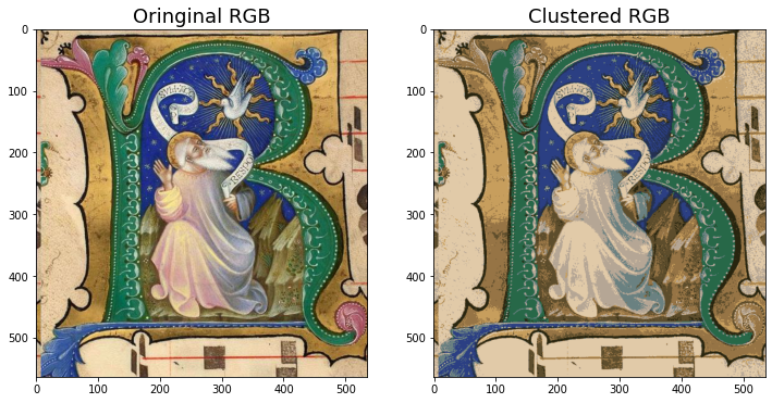
Figure 1: On the left: RGB image of Antiphonary M, folio 32; from [31]. On the right: clustered RGB with Iterative K-Means. Best value in the range $(8,12)$ at $K=11$.

We had access to the raw data of a single MA-XRF map obtained in [31], the map of Antiphonary M, folio 32 (see Figure 1).

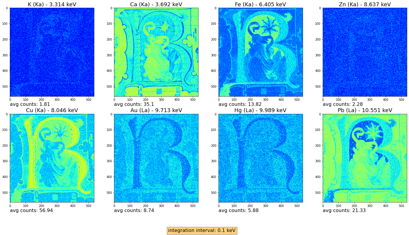
Figure 2: Examples of Elemental maps of the generated XRF with threshold $\alpha=0.2$.

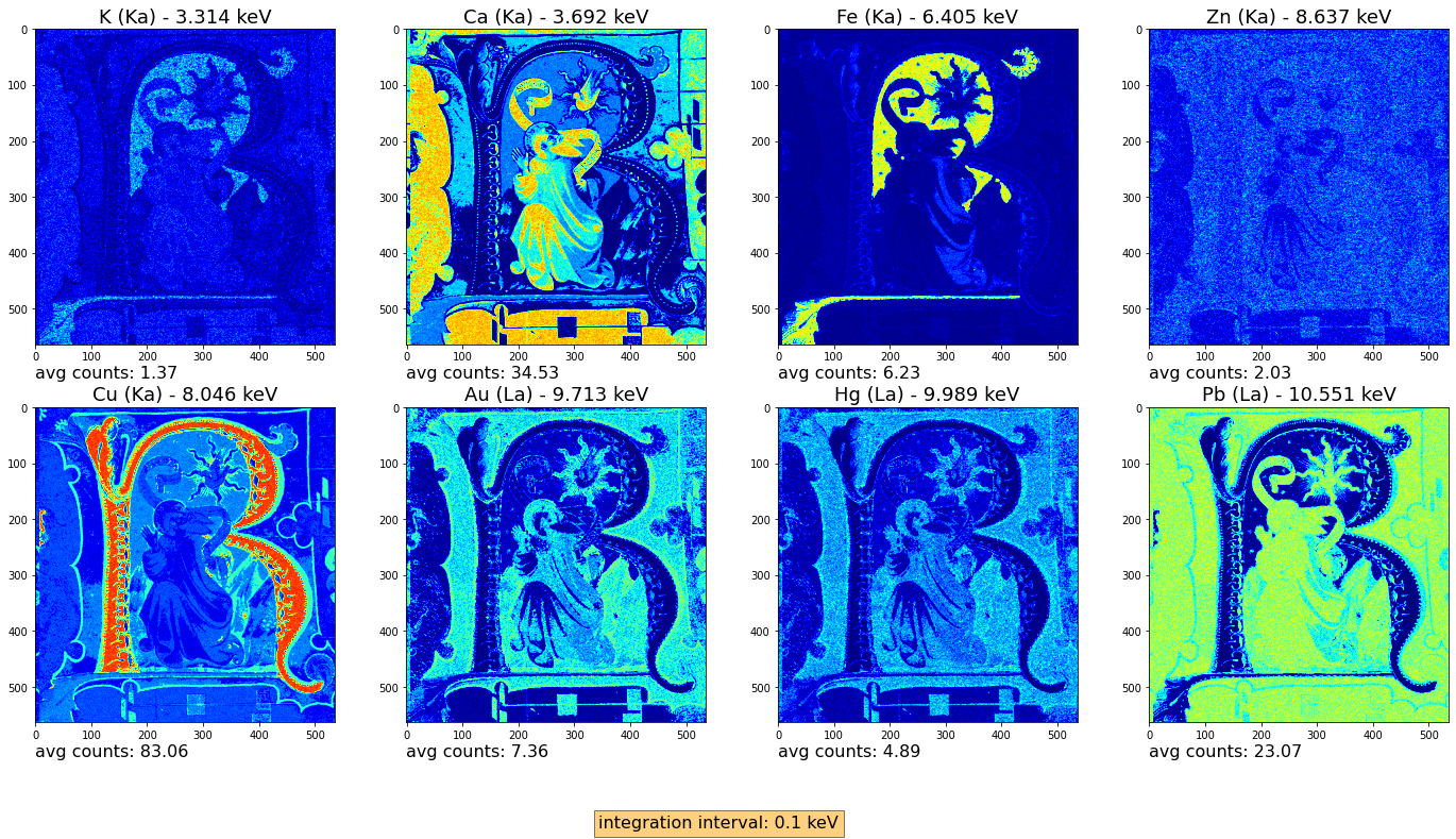
Figure 3: Examples of Elemental maps of the generated XRF with threshold $\alpha=0.6$.

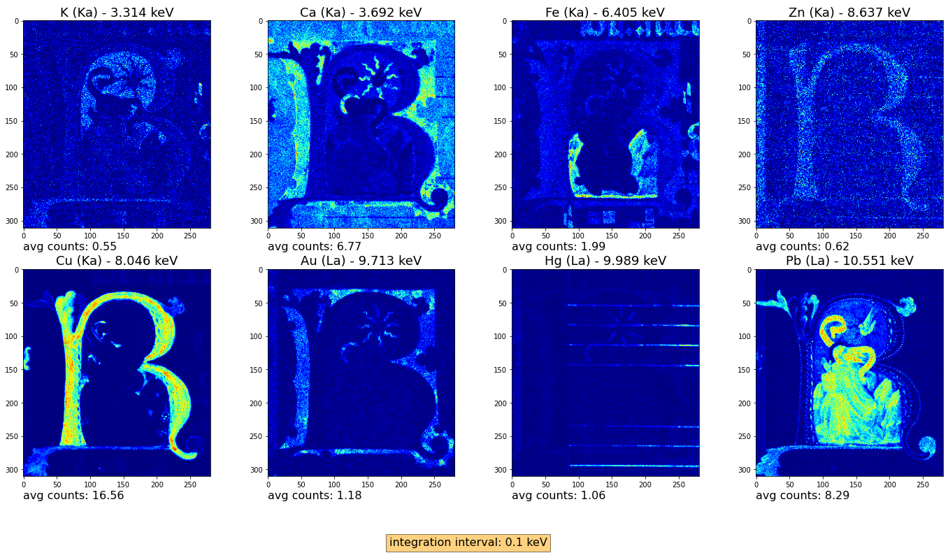
Figure 4: Examples of Elemental maps of the true XRF

We have thus generated the synthetic MA-XRF using the XRFGenerator class of ganX, and we stored it as an HDF5 file. To do so, w have used _num_of_counts$=400$, $\texttt{N\_start}=10$, $\texttt{delta\_N}=2$. $\texttt{N\_patience}=-1$, $\texttt{score\_batch}=1024$ as parameters. As an example, we have performed the generation twice: the first, with $\texttt{generation\_threshold}=0.2$; the second, with $\texttt{generation\_threshold}=0.6$. The choice was mostly random, with the intent to show how different thresholds impact the presence of pigments’ contribution in pixel counts. This is visually evident in Figures 2, 3.

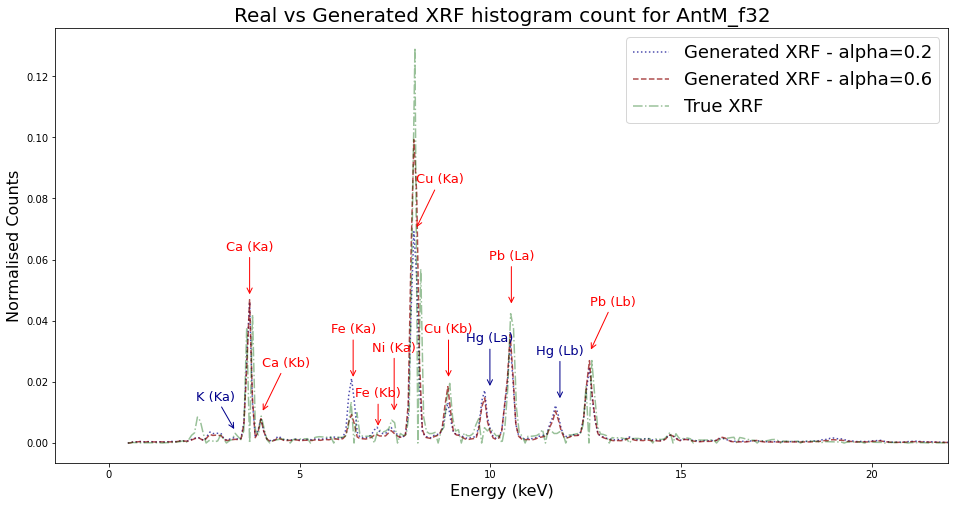
Figure 5: Comparison of the total XRF counts

To visually inspect the generated result, we computed 8 elemental maps: K (K$\alpha$), Ca (K$\alpha$), Fe (K$\alpha$), Zn (K$\alpha$), Cu (K$\alpha$), Au (L$\alpha$), Hg (L$\alpha$), Pb (L$\alpha$). The results are reported in Figures 2, 3, 4.

It is possible to give a numerical hint on the similarity between fake and true XRF in some different ways. We start by inspecting the integrated image histogram, reported in Figure 5. There are reported the generated XRF with threshold $\alpha=0.2$ histogram in dotted blue, the generated XRF with threshold $\alpha=0.6$ histogram in dashed red, and the true XRF histogram in dash-dotted green. The results for various metrics are reported in Table 1. For a brief description of the metrics, see Appendix A

Table 1: Numerical results of comparison between the fake and true XRF histograms reported in Figure 5.

	$\alpha=0.2$	$\alpha=0.6$
Cosine Distance	0.2191	0.1977
Jensen-Shannon	0.3465	0.3363
Chebyshev	0.0602	0.0817
Correlation	0.2343	0.2105
Bray-Curtis	0.3528	0.3203
Chi-square	0.3996	0.3706
Bhattacharyya	0.8529	0.8589

The yellow background metrics represent distances (i.e. the lower, the better), while the blue background metrics represent similarities (i.e. the higher, the better). Notice also that all these measures are plagued by the curse of dimensionality.

Secondly, we may flatten the XRF hypercube spatial dimensions, so that we have a 2D tensor (i.e. a matrix) of shape $(H\cdot W,E)$, where $H$ is the height, $W$ the width, and $E$ the number of energy channels. The visual comparison of those tensors are reported in Figure 6.

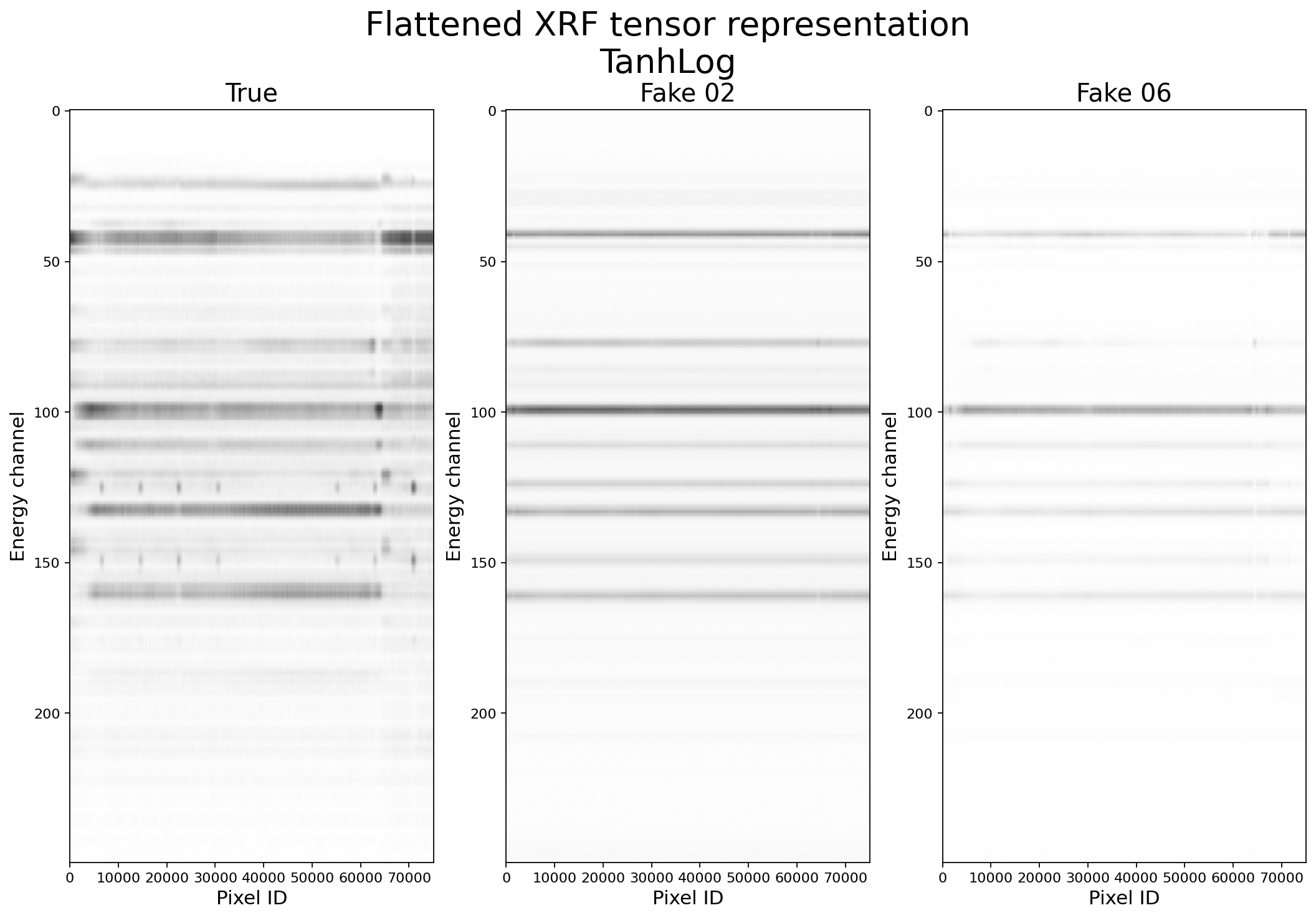
Figure 6: Flattened MA-XRF hypercubes comparison.

We have reported the binary map of the data cubes, after having applied a simple transform to enhance the visualisation of low peaks, i.e. we have mapped $x\mapsto\tanh(\log(1+x))$.

We can then use Structural Similarity Index Measure (SSIM) [32], and its multi-scale version (MS-SSIM) [33], to compute the distances among those. We also generate a random poissonian noise tensor (with the appropriate number of noise counts per pixel) as a reference measure. The results are reporte in Table 2.

Table 2: SSIM and MS-SSIM Scores for varius flattened datacubes comparison.

True vs Fake 0.2 True vs Fake 0.6 Fake 0.2 vs Fake 0.6 True vs Poisson Noise SSIM 0.3491 0.3317 0.4865 0.0878 MS_SSIM 0.4390 0.3697 0.7130 0.1597

Nevertheless, the purpose of this section was merely to illustrate the potentiality of the ganX package.

4 Conclusion

In this brief paper we have presented ganX, a Python package offering methods to generate artificial new MA-XRF data cubes out of an RGB image. This package may be helpful in the Syntethic dataset generation for applications of statistical and deep learning methods in the field of MA-XRF analysis, especially in the field of Cultural Heritage.

The next steps of the ganX package project will be to extend the flexibility of the package, by adding additional features, like to possibility to generate MA-XRF data cubes without a fixed amount of signal per-pixel, but allowing for, e.g. luminosity-based number of counts. Also, we are eploring the possibility of adding Poissonian noise, as well as other noise origin.

Furthermore, we would like to add the actual "GAN" part to ganX, i.e. creating a Generative Adversarial Network to generate the MA-XRF data cubes out of gaussian noise.

Appendix A Metrics

Here we report the definitions of the metrics used in Section 3. Notice that the histograms appearing in 5 are normalised to 1, i.e. can be seen as discrete probability distributions.

Correlation Distance:

The correlation distance between two 1D arrays $u,v$ is defined as

$$\textsc{correlation}(u,v)=1-\frac{u\cdot v}{\left\lVert(u-\bar{u})\right\rVert_{2}\,\left\lVert(v-\bar{v})\right\rVert_{2}}\,,$$ (5)

where $\bar{u},\bar{v}$ are the mean elements of $u,v$.

Cosine Distance:

The cosine distance between two 1D arrays $u,v$ is defined as

$$\textsc{cosine}(u,v)=1-\frac{u\cdot v}{\left\lVert u\right\rVert_{2}\,\left\lVert v\right\rVert_{2}}\,.$$ (6)

The cosine distance is related to the angle $\theta$ between the vectors $u,v\in\mathbb{R}^{N}$, i.e.

$$\cos\theta=\frac{u\cdot v}{\left\lVert u\right\rVert_{2}\,\left\lVert v\right\rVert_{2}}=1-\textsc{cosine}(u,v)\,.$$ (7)

Jensen - Shannon:

The Jensen-Shannon distance between two normalised 1D arrays $u,v$ is defined as

$$\textsc{JensenShannon}(u,v)=\sqrt{\frac{D_{KL}(u||m)+D_{KL}(v||m)}{2}}\,.,$$ (8)

where $m$ is the pointwise mean of $u$ and $v$ and $D_{KL}$ is the Kullback-Leibler divergence (or relative entropy), i.e.

$$D_{KL}(P||Q)=\sum_{n=1}^{N}P(n)\log\frac{P(n)}{Q(n)}\,.$$ (9)

Chebyshev:

The Chebyshev distance between two 1D arrays $u,v$ is defined as

$$\textsc{Chebyshev}(u,v)=\max_{i}\left|u_{i}-v_{i}\right|\,.$$ (10)

Bray-Curtis:

The Bray-Curtis dissimilarity between two 1D arrays $u,v$ is defined as

$$\textsc{BrayCurtis}(u,v)=\sum_{n=1}^{N}\frac{\left|u_{n}-v_{n}\right|}{\left|u_{n}+v_{n}\right|}\,.$$ (11)

Chi-quare

The Chi-square distance between two 1D arrays $u,v$ is defined as

$$\chi^{2}(u,v)=\frac{1}{2}\,\sum_{n=1}^{N}\frac{\left(u_{n}-v_{n}\right)^{2}}{\left|u_{n}+v_{n}\right|}\,.$$ (12)

Bhattacharyya:

The Bhattacharyya coefficient BC between two 1D arrays $u,v$ is defined as

$$\textsc{BC}(u,v)=\sum_{n=1}^{N}\sqrt{u_{n}v_{n}}\,.$$ (13)

The Bhattacharyya coefficient can be also used to compute the Bhattacharyya distance $\textsc{D}_{B}$

$$\textsc{D}_{B}(u,v)=-\log\textsc{BC}(u,v)\,,$$ (14)

as well as the Hellinger distance $H$

$$H(u,v)=\sqrt{1-\textsc{BC}(u,v)}\,.$$ (15)

References

- [1] Haohan Wang and Bhiksha Raj. On the origin of deep learning, 2017.
- [2] Ian Goodfellow, Yoshua Bengio, and Aaron Courville. Deep Learning. MIT Press, 2016. http://www.deeplearningbook.org.
- [3] Aston Zhang, Zachary C. Lipton, Mu Li, and Alexander J. Smola. Dive into deep learning, 2021.
- [4] Tania Kleynhans, Catherine M. Schmidt Patterson, Kathryn A. Dooley, David W. Messinger, and John K. Delaney. An alternative approach to mapping pigments in paintings with hyperspectral reflectance image cubes using artificial intelligence. Heritage Science, 8(1):84, Aug 2020.
- [5] Giorgio A. Licciardi and Fabio Del Frate. Pixel unmixing in hyperspectral data by means of neural networks. IEEE Transactions on Geoscience and Remote Sensing, 49(11):4163–4172, 2011.
- [6] Xiangrong Zhang, Yujia Sun, Jingyan Zhang, Peng Wu, and Licheng Jiao. Hyperspectral unmixing via deep convolutional neural networks. IEEE Geoscience and Remote Sensing Letters, 15(11):1755–1759, 2018.
- [7] Mou Wang, Min Zhao, Jie Chen, and Susanto Rahardja. Nonlinear unmixing of hyperspectral data via deep autoencoder networks. IEEE Geoscience and Remote Sensing Letters, 16(9):1467–1471, 2019.
- [8] Sotiria Kogou, Lynn Lee, Golnaz Shahtahmassebi, and Haida Liang. A new approach to the interpretation of XRF spectral imaging data using neural networks. X-Ray Spectrometry, 50(4), 2020.
- [9] Lingxi Liu, Tsveta Miteva, Giovanni Delnevo, Silvia Mirri, Philippe Walter, Laurence de Viguerie, and Emeline Pouyet. Neural networks for hyperspectral imaging of historical paintings: A practical review. Sensors, 23(5), 2023.
- [10] Qiqin Dai, Henry Chopp, Emeline Pouyet, Oliver Cossairt, Marc Walton, and Aggelos K. Katsaggelos. Adaptive image sampling using deep learning and its application on X-Ray fluorescence image reconstruction. CoRR, abs/1812.10836, 2018.
- [11] Alessandro Bombini, Lucio Anderlini, Luca dell’Agnello, Francesco Giacomini, Chiara Ruberto, and Francesco Taccetti. The AIRES-CH Project: Artificial Intelligence for Digital REStoration of Cultural Heritages Using Nuclear Imaging and Multidimensional Adversarial Neural Networks. In Stan Sclaroff, Cosimo Distante, Marco Leo, Giovanni M. Farinella, and Federico Tombari, editors, Image Analysis and Processing – ICIAP 2022, pages 685–700, Cham, 2022. Springer International Publishing.
- [12] Alessandro Bombini, Lucio Anderlini, Luca dell’Agnello, Francesco Giacomini, Chiara Ruberto, and Francesco Taccetti. Hyperparameter Optimisation of Artificial Intelligence for Digital REStoration of Cultural Heritages (AIRES-CH) Models. In Osvaldo Gervasi, Beniamino Murgante, Sanjay Misra, Ana Maria A. C. Rocha, and Chiara Garau, editors, Computational Science and Its Applications – ICCSA 2022 Workshops, pages 91–106, Cham, 2022. Springer International Publishing.
- [13] Marc Vermeulen, Alicia McGeachy, Bingjie Xu, Henry Chopp, Aggelos Katsaggelos, Rebecca Meyers, Matthias Alfeld, and Marc Walton. XRFast a new software package for processing of MA-XRF datasets using machine learning . J. Anal. At. Spectrom., 37:2130–2143, 2022.
- [14] Cerys Jones, Nathan S. Daly, Catherine Higgitt, and Miguel R. D. Rodrigues. Neural network-based classification of x-ray fluorescence spectra of artists’ pigments: an approach leveraging a synthetic dataset created using the fundamental parameters method. Heritage Science, 10(1):88, Jun 2022.
- [15] Xu Bingjie, Yunan Wu, Pengxiao Hao, Marc Vermeulen, Alicia McGeachy, Kate Smith, Katherine Eremin, Georgina Rayner, Giovanni Verri, Florian Willomitzer, Matthias Alfeld, Jack Tumblin, Aggelos Katsaggelos, and Marc Walton. Can deep learning assist automatic identification of layered pigments from xrf data?, 2022.
- [16] Su Yan, Jun-Jie Huang, Nathan Daly, Catherine Higgitt, and Pier Luigi Dragotti. When de prony met leonardo: An automatic algorithm for chemical element extraction from macro x-ray fluorescence data. IEEE Transactions on Computational Imaging, 7:908–924, 2021.
- [17] Alessandro Bombini. ganX - generate artificially new XRF, 1 2023. https://github.com/androbomb/ganX.
- [18] Jacob Sherman. The theoretical derivation of fluorescent x-ray intensities from mixtures. Spectrochimica acta, 7:283–306, 1955.
- [19] Stéfan van der Walt, S Chris Colbert, and Gaël Varoquaux. The NumPy array: A structure for efficient numerical computation. Computing in Science & Engineering, 13(2):22–30, mar 2011.
- [20] Charles R. Harris, K. Jarrod Millman, Stéfan J. van der Walt, Ralf Gommers, Pauli Virtanen, David Cournapeau, Eric Wieser, Julian Taylor, Sebastian Berg, Nathaniel J. Smith, Robert Kern, Matti Picus, Stephan Hoyer, Marten H. van Kerkwijk, Matthew Brett, Allan Haldane, Jaime Fernández del Río, Mark Wiebe, Pearu Peterson, Pierre Gérard-Marchant, Kevin Sheppard, Tyler Reddy, Warren Weckesser, Hameer Abbasi, Christoph Gohlke, and Travis E. Oliphant. Array programming with NumPy. Nature, 585(7825):357–362, September 2020.
- [21] J. MacQueen. Some methods for classification and analysis of multivariate observations. Proc. 5th Berkeley Symp. Math. Stat. Probab., Univ. Calif. 1965/66, 1, 281-297 (1967)., 1967.
- [22] F. Pedregosa, G. Varoquaux, A. Gramfort, V. Michel, B. Thirion, O. Grisel, M. Blondel, P. Prettenhofer, R. Weiss, V. Dubourg, J. Vanderplas, A. Passos, D. Cournapeau, M. Brucher, M. Perrot, and E. Duchesnay. Scikit-learn: Machine learning in Python. Journal of Machine Learning Research, 12:2825–2830, 2011.
- [23] Peter J. Rousseeuw. Silhouettes: A graphical aid to the interpretation and validation of cluster analysis. Journal of Computational and Applied Mathematics, 20:53–65, 1987.
- [24] L. Kaufman and P. J. Rousseeuw. Finding Groups in Data: An Introduction to Cluster Analysis. A Wiley-Interscience publication. Wiley, 1990.
- [25] M. R. Luo, G. Cui, and B. Rigg. The development of the cie 2000 colour-difference formula: Ciede2000. Color Research & Application, 26(5):340–350, 2001.
- [26] Gaurav Sharma, Wencheng Wu, and Edul N. Dalal. The ciede2000 color-difference formula: Implementation notes, supplementary test data, and mathematical observations. Color Research & Application, 30(1):21–30, 2005.
- [27] Stéfan van der Walt, Johannes L. Schönberger, Juan Nunez-Iglesias, François Boulogne, Joshua D. Warner, Neil Yager, Emmanuelle Gouillart, and Tony Yu. scikit-image: image processing in python. PeerJ, 2:e453, jun 2014.
- [28] M. Melgosa, J. J. Quesada, and E. Hita. Uniformity of some recent color metrics tested with an accurate color-difference tolerance dataset. Appl. Opt., 33(34):8069–8077, Dec 1994.
- [29] Alan R. Robertson. The cie 1976 color-difference formulae. Color Research & Application, 2(1):7–11, 1977.
- [30] I. M. Cortea, L. M. Chiro\textcommabelowsca, L. M. Anghelu\textcommabelowtă, and G. Seri\textcommabelowtan. INFRA-ART: An Open Access Spectral Library of Art-Related Materials as a Digital support Tool for Cultural Heritage Science. ACM Journal on Computing and Cultural Heritage, 16(2), 2023.
- [31] Paola Ricciardi, Anna Mazzinghi, Stefano Legnaioli, Chiara Ruberto, and Lisa Castelli. The Choir Books of San Giorgio Maggiore in Venice: Results of in Depth Non-Invasive Analyses. Heritage, 2(2):1684–1701, 2019.
- [32] Zhou Wang, A.C. Bovik, H.R. Sheikh, and E.P. Simoncelli. Image quality assessment: from error visibility to structural similarity. IEEE Transactions on Image Processing, 13(4):600–612, 2004.
- [33] Z. Wang, E.P. Simoncelli, and A.C. Bovik. Multiscale structural similarity for image quality assessment, 2003.