Structured level/̄2 condition numbers of matrix functions††thanks: Received by the editors on Month/Day/Year. Accepted for publication on Month/Day/Year. Handling Editor: Name of Handling Editor. Corresponding Author: Marcel Schweitzer
Abstract
Matrix functions play an increasingly important role in many areas of scientific computing and engineering disciplines. In such real-world applications, algorithms working in floating-point arithmetic are used for computing matrix functions and additionally, input data might be unreliable, e.g., due to measurement errors. Therefore, it is crucial to understand the sensitivity of matrix functions to perturbations, which is measured by condition numbers. However, the condition number itself might not be computed exactly as well due to round-off and errors in the input. The sensitivity of the condition number is measured by the so-called level/̄2 condition number. For the usual (level-1) condition number, it is well-known that structured condition numbers (i.e., where only perturbations are taken into account that preserve the structure of the input matrix) might be much smaller than unstructured ones, which, e.g., suggests that structure-preserving algorithms for matrix functions might yield much more accurate results than general-purpose algorithms. In this work, we examine structured level/̄2 condition numbers in the particular case of restricting the perturbation matrix to an automorphism group, a Lie or Jordan algebra or the space of quasi-triangular matrices. In numerical experiments, we then compare the unstructured level/̄2 condition number with the structured one for some specific matrix functions such as the matrix logarithm, matrix square root, and matrix exponential.
keywords:
level/̄2 condition number, matrix function, automorphism group, Lie algebra, Jordan algebra, quasi-triangular matrices65F35, 15A16, 65F60
1 Introduction
Matrix functions , where or , such as the matrix exponential, logarithm, and square root are used in a wide variety of applications including the solution of differential equations by exponential integrators, network analysis and machine learning [4, 6, 8, 16, 20, 23, 28]. The condition number measures the sensitivity of a matrix function to perturbations in the input due to rounding or measurement error.
The (level-1) absolute condition number is defined for a matrix function as
| (1.1) |
It can be computed via the Fréchet derivative of the matrix function, a linear function in the perturbation matrix such that satisfies [19, Section 3]
as we outline at the beginning of section 2.1. When the input matrix has some structure described by a Lie or Jordan algebra (e.g. symmetric or skew-Hermitian), and we consider only perturbations that retain this structure, the resulting structured level-1 condition number can be significantly smaller. This has been investigated in [31] for linear systems, matrix inversion, and distance to singularity. The effect of structured perturbations of matrix functions in Lie and the Jordan algebras is also studied by Davies [10]. The structured level-1 condition number using differentials between smooth manifolds is also analysed for automorphism groups in [7].
Unfortunately, the condition number itself might not be computed precisely: previous work on the condition number of the condition number (the so-called level/̄2 condition number) [22] has shown that it can be highly sensitive in some cases. Similar findings are also known for the level/̄2 condition number for solving linear systems [13, 17].
The aim of this work is to investigate the structured level/̄2 condition number of matrix functions by enforcing structure on the perturbation matrices and it is organised as follows. In section 2 we summarise existing work on the unstructured level/̄2 condition number of matrix functions and the structured level-1 condition number. We then build upon these foundations in section 3 and derive upper bounds for structured condition numbers of matrix functions of different structures. We first investigate the case of matrices coming from Lie and Jordan algebras or automorphism groups and then focus on the important case of quasi-triangular matrices. Additionally, for a few specific choices of function and matrix class, we derive exact formulas for the structured level/̄2 condition number. Numerical experiments in section 4 provide a thorough comparison of the structured and unstructured condition numbers for the matrix exponential, logarithm, and square root over a variety of structures. We summarise our findings in section 5 and give some ideas for future work in this area.
2 Previous work on matrix function conditioning
In this section we summarise the current theory on matrix function conditioning, which we build upon to derive corresponding results for the structured level/̄2 condition number in later sections. In particular, we focus here on the structured level-1 condition number and the unstructured level/̄2 condition number. We reproduce some of the derivations in quite a bit of detail, as the concepts and notations introduced there are essential for understanding the derivations of our new results in section 3.
2.1 The unstructured level/̄2 condition number case
In this section we summarise previous results for the unstructured level/̄2 condition number, largely based upon [19] and [22]. To begin, the level-1 condition number is the norm of the first order Fréchet derivative operator , i.e.,
where can in principle be any matrix norm. It is convenient to use the Frobenius norm because of the fact that , where stacks the columns of a matrix into one long vector. This reduces the problem to finding the 2-norm of , the Kronecker form of the Fréchet derivative: The Kronecker form is the matrix of size that satisfies
Using this definition, the condition number in the Frobenius norm can be rewritten as
Higher order derivatives of matrix functions are defined similarly, and in particular the second Fréchet derivative is a multilinear function which satisfies
| (2.2) |
Sufficient conditions for the existence of the second Fréchet derivative are given by Higham and Relton [22, Theorem 3.5]. This theorem also states that is equal to the upper right block of ,
| (2.3) |
where is built using the following recursion
with the identity matrix and the Kronecker product.
Using these building blocks, one can define higher-order condition numbers of matrix functions which capture the sensitivity of the condition number itself to perturbations in . We outline the basic approach here, following largely the derivation in [22]. We begin by defining the absolute level/̄2 condition number via the following equation,
| (2.4) |
We can derive an upper bound for the level/̄2 condition number (see [22]) by combining equations (1.1) and (2.2), which yields
From the triangular inequality we get the upper bound
Using this within the definition of the level/̄2 condition number (2.4) yields
| (2.5) |
where the supremum can be replaced with a maximum in a finite dimensional vector space and since is linear in we can have . Furthermore, as is also linear in , there exists a matrix such that
Using these facts and taking the Frobenius norm in the upper bound (2.5) leads to
| (2.6) |
where is the Kronecker form of the second Fréchet derivative.
We stress that—in contrast to the level-1 condition number—the spectral norm of the Kronecker form only gives an upper bound for the level/̄2 condition number instead of its precise value. The exact value of the level/̄2 condition number can only be determined in certain special cases. Higham and Relton find formulas for the exact level/̄2 condition number for the matrix inverse [22, Section 5.2] and the exponential of normal matrices [22, Section 5.1], while Schweitzer finds an exact formula for certain functions of Hermitian matrices which have a strictly monotonic derivative [30, Section 3].
2.2 The structured case
In this subsection we give a brief recap of the framework within which structured perturbations can be analysed, and proceed to derive similar results to the above for structured matrices.
Let be a smooth square matrix manifold for a field . For a smooth manifold , the element is a tangent vector of at if there is a smooth curve such that , . The set
| (2.7) |
is called the tangent space of at . Furthermore we define a scalar product, from to : for any nonsingular matrix by,
Finally, for any matrix , there exists a unique , called the adjoint of with respect to the scalar product , which is given by
We are interested in three classes of structured matrices associated with : a Jordan algebra , a Lie algebra and an automorphism group defined by
respectively. Practically important choices of are given by the three matrices
| (2.8) |
as , and then correspond to some commonly encountered matrix structures; cf. Table 1. Note that for all choices of from (2.8), we trivially have that with .
| Real/Complex Bilinear forms | |||
|---|---|---|---|
| M | Automorphism Group () | Jordan Algebra () | Lie Algebra () |
| Real orthogonals | Symmetrics | Skew-symmetrics | |
| Complex orthogonals | Complex symmetrics | Complex skew-symmetrics | |
| Pseudo-orthogonals | Pseudo-symmetrics | Pseudo skew-symmetrics | |
| Complex pseudo-orthogonals | Complex pseudo-symmetrics | Complex pseudo-skew-symmetrics | |
| Real perplectics | Persymmetric | Perskew-symmetrics | |
| Real symplectics | Skew-Hamiltonians | Hamiltonians | |
| Complex symplectics | -skew-symmetric | -symmetrics | |
With these fundamentals, we are ready to define the structured level-1 condition number using differentials between tangent spaces to smooth square matrix manifolds, closely following [7].
Definition 2.1.
Let be a smooth matrix function between two smooth square matrix manifolds and . Let be such that is defined. Then the absolute structured level-1 condition number of is
| (2.9) |
The enforced condition restricts the choice of the perturbation to a smaller set than in the unstructured case, so from the definition of the supremum, we get
The structured condition number can equivalently be expressed in terms of the differential of . Precisely, if is -differentiable, then the differential of at the point is the map
where and are tangent spaces as defined in (2.7). Using this definition, it holds
| (2.10) |
where
For practically computing the structured level-1 condition number, one constructs a structured equivalent of the Kronecker form: Let the columns of span the tangent space and let with . Then for we have . Focusing on the Frobenius norm as before, the structured level-1 condition number can be expressed as
where denotes the Moore–Penrose pseudoinverse of . The construction of the tangent space basis is given in [7, Section 3.1], which shows that for we can construct the basis of the tangent space of and as
| (2.11) |
with
where if , if and is a matrix with the columns
and has the column vectors , .
For an automorphism group the basis of the tangent space to at is given by
| (2.12) |
cf. [7, Section 3.2].
3 New results
In this section, we derive our main result, Lemma 3.1, and use it to find upper bounds for structured level/̄2 condition numbers for various different matrix structures in section 3.1 and 3.2. In section 3.3 we discuss two particular cases in which it is possible to exactly compute the structured level/̄2 condition number. In section 3.4, we also comment on how to numerically compute lower bounds for level/̄2 condition numbers, which are required for judging the quality of the upper bounds we obtained.
3.1 The level/̄2 condition number of matrices from Lie and Jordan algebras or automorphism groups
For a smooth matrix function we can define the structured level/̄2 condition number similarly to (2.4), but restricting the perturbation matrix to ,
| (3.13) |
The following lemma provides an upper bound of the structured level/̄2 condition number of .
Lemma 3.1.
Let be a smooth matrix function between two smooth square matrix manifolds and . Let be such that is defined. Then an upper bound for the structured level/̄2 condition number of is given by
| (3.14) |
where the columns of span , the tangent space of at .
Proof 3.2.
Using the first and the second Fréchet derivatives gives
Enforcing the structure on the perturbation matrices and with yields the following upper bound of the structured level/̄2 condition number:
| (3.15) |
where, for the last equality, we used the fact that together with the definition of the 2-norm,
Bounding the 2-norm by the Frobenius norm, we further obtain, starting from (3.15),
again using .
We now modify [22, Algorithm 4.2] to obtain an upper bound for the structured level/̄2 condition number. It requires any algorithm to compute for , where is a smooth matrix manifold and , i.e., for some , and returns . The resulting method is depicted in Algorithm 1.
We briefly comment on the computational cost of Algorithm 1: For typical practically relevant matrix functions, algorithms are available for evaluating them at a cost of . These also directly transfer (via the relation (2.3)) to algorithms for computing at cost , albeit with an additional constant hidden in the , as the matrix in (2.3) is of size . Thus, the overall cost of the algorithm is , where is the dimension of the tangent space and the constant can be expected to be quite large. This makes the algorithm prohibitively expensive even for medium scale problems (a typical limitation that is also already present when computing unstructured level/̄2 or even level-1 condition numbers).
The computational cost of individual Fréchet derivative evaluations can be reduced somewhat by using complex-step approximations [2] or quadrature-based algorithms [30]. While in general, when and the are unstructured, this does not change the asymptotic scaling of Algorithm 1, experiments in [30] indicate that run time can be reduced by about one order of magnitude. If the direction terms are rank-one matrices (which, e.g., happens if the columns of are certain canonical unit vectors), then run time of Algorithm 1 can potentially be reduced to if linear systems with can be solved efficiently; see [30, Section 4.3] for details.
3.2 The level/̄2 condition number of (quasi-)triangular matrices
Another type of matrix structure that differs from those considered in section 2.2 and 3.1 is (quasi-)triangularity, which plays an important role in many algorithms for computing matrix functions. An upper quasi-triangular matrix is a block upper triangular matrix with diagonal blocks of size at most . These commonly occur when using the Schur decomposition: For general , a Schur decomposition with unitary and upper triangular is always guaranteed to exist. Note, however, that and may be complex-valued even if is real. In the case of real-valued , one can instead use a real Schur decomposition , where the matrices and are both real-valued, but is now upper quasi-triangular.
Given a (real) Schur decomposition, the relation shows that evaluating can essentially be reduced to the evaluating at a (quasi-)triangular matrix. This forms the basis of many numerical methods for computing at small and dense matrices : the Schur–Parlett algorithm [11, 21], for example.
Structured level-1 condition numbers of have recently been investigated in [1], and we extend this concept to the level/̄2 case. Quasi-triangular matrices do not fit into the framework of Lie and Jordan algebras or automorphism groups induced by a scalar product, and have an arguably simpler structure. We recall some important properties:
-
1.
The set of quasi-triangular matrices (with a fixed structure of diagonal blocks) forms a subalgebra of and is thus in particular a linear space and a smooth matrix manifold.
-
2.
As is a linear space, we have for any .
-
3.
As any matrix function is a polynomial in and is a subalgebra of , we have , i.e., a function of a quasi-triangular matrix is a quasi-triangular matrix with the same diagonal block structure.
In light of the above observations, Lemma 3.1 also applies to the case of quasi-triangular matrices, and for we can take a basis of the space of upper quasi-triangular matrices (with the induced block structure). Such a basis is easily constructed from canonical unit vectors: Using the notation introduced in [1], let denote a vector that encodes the diagonal block structure of , i.e.,
To clearly indicate that the block structure is fixed, we denote the algebra of all quasi-triangular matrices with block structure encoded by as . Clearly, , where denotes the number of nonzero entries. A (vectorised) basis of is given by
| (3.16) |
The basis (3.16) is orthonormal by construction, so if we take these basis vectors as columns of , we have .
3.3 Exact structured level/̄2 condition numbers for special cases
So far, we were only able to determine upper bounds for the structured level/̄2 condition number, which is in general all one can hope to obtain. However, for a few particular combinations of matrix class, function and used norm, it is possible to give an exact, closed form for .
Exponential of skew-Hermitian matrices
When using the spectral norm (instead of the Frobenius norm that is typically employed), one can exactly compute the structured level/̄2 condition number when comes from the Lie Algebra of skew-Hermitian matrices. Note that exponentials of skew-Hermitian matrices, e.g., play an important role in the simulation of quantum systems, where according to the Schrödinger equation, the evolution of states is governed by , where is the (Hermitian) Hamiltonian of the system; see, e.g., [27]. As a special case of the very general result that the exponential map takes a Lie algebra into its corresponding Lie group, it is well-known that the exponential of a skew-Hermitian matrix is unitary, a property that is fundamental for proving the following result.
Proposition 3.3.
Let be skew-Hermitian. Then, in the spectral norm,
Proof 3.4.
By a result from [32, Section 4] for the unstructured condition number, it holds for any normal matrix that in the spectral norm , where denotes the largest real part of any eigenvalue of (the so-called spectral abscissa). Any skew-Hermitian matrix is normal and has eigenvalues on the imaginary axis, so that , and therefore . We now argue that the same holds for the structured level-1 condition number, i.e., . Consider the skew-Hermitian matrix . We then have and . Taking this into account, we find
| (3.17) |
where we have used in the second to last equality that is unitary and therefore has spectral norm equal to one. From (3.17) it follows that the supremum in (2.9) is at least one. On the other hand, the structured condition number is always bounded above by the unstructured one, so they must agree. Using this, the assertion of the proposition directly follows: From the definition (3.13), we have
where we have used that is again skew-Hermitian.
Exponential of Hermitian matrices
Next, we investigate the Hermitian case. As in the skew-Hermitian case, the structured and unstructured level-1 condition numbers agree, and this time, this carries over to the level/̄2 condition numbers.
Proposition 3.5.
Let be Hermitian. Then, in the spectral norm,
where denotes the largest eigenvalue of .
Proof 3.6.
Proceeding as in the proof of Proposition 3.3, we have that . According to [22, Theorem 5.2], it also holds that . Clearly, for any Hermitian with we have , as the spectral norm of a Hermitian matrix is simply its largest eigenvalue. The upper bound is attained for the Hermitian matrix , and it follows from the definition of the structured level/̄2 condition number that
Remark 3.7.
One might argue that the results of Proposition 3.3 and 3.5 are of limited practical relevance. However, they highlight quite interesting properties and difficulties related to level/̄2 (structured) condition numbers: In both cases, the structured and unstructured level-1 condition numbers agree, but the implications for the level/̄2 condition number are fundamentally different. While in the Hermitian case, the structured and unstructured level/̄2 condition number also always agree, they can never be equal in the skew-Hermitian case (the level/̄2 unstructured condition number of the exponential of a skew-Hermitian matrix is always equal to according to [22, Theorem 5.2]). As the structured condition number is zero, this even shows that without additional assumptions, it is impossible to derive any meaningful bounds on the ratio between the unstructured and structured condition number,
with for relating the structured and unstructured condition numbers (i.e., in general, the unstructured condition number can be “infinitely worse” than the structured one).
3.4 Lower bounds for the unstructured level/̄2 condition number
One fundamental difficulty in gauging the quality of the results obtained in sections 3.1 and 3.2 is that there is no known algorithm to compute the exact level/̄2 condition number (in either the structured or unstructured case) except for very particular special cases where analytic forms are known; see the discussion at the end of section 2.2 for the unstructured case and section 3.3 above for the structured one. Thus, instead of comparing the structured level/̄2 condition number to the unstructured level/̄2 condition number we can only compare upper bounds for both quantities.
This has a fundamental limitation in that we do not know the sharpness of the bounds: if an arbitrary upper bound for quantity lies below an arbitrary upper bound for quantity , this does not tell us anything about the relation between and . Thus, even when (3.14) lies orders of magnitude below (2.6), this does not necessarily mean that and are different. Of course, one can intuitively expect that both bounds (2.6) and (3.14) are similar in quality as they originate in strongly related concepts, but this is not guaranteed.
In order to obtain more robust results, we also compute lower bounds for the level/̄2 condition numbers in our experiments: If an upper bound for the structured condition number lies well below a lower bound for the unstructured condition number, then this is clearly also the case for the exact quantities, which must differ by at least the same amount. To obtain lower bounds, observe that in light of (2.4), for any particular matrix with we clearly have
| (3.18) |
Thus, the right-hand side of (3.18) gives a lower bound of the unstructured condition number for any fixed . Clearly, a similar relation also holds for the structured condition number, provided that is chosen from the according tangent space.
To obtain lower bounds in our experiments, we use the MATLAB built-in function fminsearch, which implements the derivative-free simplex search method from [26] for maximising the right-hand side of (3.18) by choosing . Within our numerical experiments, we replace the limit and use a finite difference quotient instead, with . Strictly speaking, what we obtain this way is only an approximate lower bound, but a comparison to the upper bounds indicates that the result of the optimisation procedure is reliable.
4 Numerical Experiments

The aim of this section is to compare the structured and unstructured level/̄2 condition numbers for the matrix logarithm, matrix square root and matrix exponential. As these cannot be computed exactly, we compare the upper bounds from sections 2.1, 3.1 and 3.2, as well as the approximate lower bounds from section 3.4.
We use MATLAB R2022a on a machine with an AMD Ryzen 7 3700X 8-core CPU to run the experiments. We build test matrices as follows.
-
•
Orthogonal, symplectic and perplectic matrices are built using Jagger’s toolbox [24].
-
•
Hamiltonian matrices are built as
-
•
Quasi-triangular matrices are artificially generated as follows: We generate a diagonal matrix with equidistantly distributed entries in the interval for a specified parameter . We then compute with a randomly sampled matrix and perform a real Schur decomposition to obtain the upper quasi-triangular matrix .
-
•
Alternatively, we obtain quasi-triangular matrices by performing a (real) Schur decomposition of a large set of common benchmark matrices from the matrix function literature; see Appendix A for details on the test set.
Depending on the matrix function we construct using either equation or .
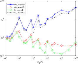
The upper bounds for the structured and unstructured level/̄2 condition numbers are computed using Algorithm 1 and equation (2.6), respectively. For symplectic, perplectic and quasi-triangular matrices the bounds are plotted against the 2-norm condition number for matrix inversion, , whereas for orthogonal matrices we sort the test matrices by increasing values of the unstructured condition number. Within the legend of each plot the acronyms ub and lb are used to indicate upper and lower bounds, meanwhile scond2 and uscond2 denote the structured and unstructured level/̄2 condition numbers.
-
Experiment 4.1.
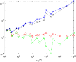
We first consider the matrix logarithm and by taking we construct using equation (2.12). In Algorithm 1 we compute the matrix logarithm by the MATLAB function logm which uses the improved inverse scaling and squaring method [5]. The upper bounds for the structured and unstructured level/̄2 condition numbers are shown in Figure 1 for orthogonal, symplectic and perplectic matrices . Comparing the results obtained from different test matrices, we observe that in particular in the symplectic and perplectic case, the structured condition number is much smaller than the unstructured one (in fact, the structured level/̄2 condition number appears to stay almost constant across all considered test matrices). In the orthogonal case, the difference is less pronounced, but can still be observed clearly. Both the magnitude as well as the slope at which it increases are substantially smaller for the structured level/̄2 condition number.
The lower bounds that we also report confirm that in most cases, our upper bounds are quite tight and the structured condition number is indeed guaranteed to be much smaller than the unstructured one. Let us briefly comment on the fact that for the most ill-conditioned symplectic and perplectic matrices, the lower bound for the unstructured condition number that we report lies above the upper bound. This is likely caused by the fact that it is actually only an approximate lower bound (cf. the discussion in section 3.4) combined with the severe ill-conditioning of the matrix under consideration. Apart from this, our results (also those reported in later experiments) still indicate that in general the lower bounds can be expected to be quite reliable.
-
Experiment 4.2.
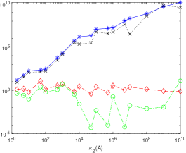
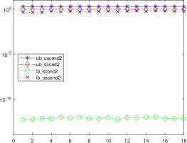
We take the matrix square root and is built by equation (2.12). For computing the matrix square root we use sqrtm which is based on the method given in [12]. The bounds are shown in Figure 2 for orthogonal, symplectic and perplectic matrices . We observe similar results as in the previous experiment. In particular, there is a dramatic increase in the unstructured level/̄2 condition numbers for ill-conditioned matrices, while the structured one again stays roughly constant for symplectic and perplectic matrices and only increases moderately for orthogonal matrices.
The lower bounds again confirm that our results are reliable and show that the upper bounds are quite tight, in particular in the symplectic and perplectic case.
-
Experiment 4.3.
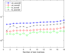
In this experiment we consider the matrix exponential for skew-symmetric and Hamiltonian matrices . We again construct by equation (2.11) and use the MATLAB function expm, which is based on a scaling and squaring algorithm [3] to compute the exponential. Figure 3 demonstrates that the upper bounds for the structured and unstructured level/̄2 condition number behave very similarly in both cases, with the bounds for the unstructured condition number being almost exactly two times as large as the structured one for both kinds of test matrices. In light of Proposition 3.3 (although this result uses the spectral norm and not the Frobenius norm as in this experiment), it is interesting to observe that in the skew-symmetric case, the lower bound stays in the order of . This value close to machine precision appears to confirm that the exact value is zero.
-
Experiment 4.4.
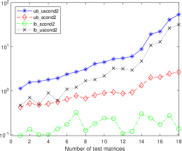
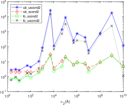
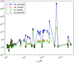
We take randomly generated (as described at the beginning of this section) upper quasi-triangular matrices , with the parameter ranging between and and . Note that we increase the matrix size compared to the previous experiments to allow for more variety in the diagonal block structure of . We compute the upper bounds (2.6) and (3.14) as well as lower bounds for the structured and unstructured level/̄2 condition number. The results are depicted on the left-hand side of Figure 4. As it was the case for the other considered matrix structures, the bounds again confirm that structured level/̄2 conditioning can be much better than unstructured conditioning, in particular for the more ill-conditioned examples. The lower bounds obtained by optimisation are also mostly very tight.
-
Experiment 4.5.
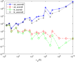
In the final experiment, instead of randomly generating matrices, we compute bounds for the structured and unstructured level/̄2 condition numbers of , where is taken as the upper quasi-triangular factor of the (real) Schur decomposition of a wide range of matrices from the matrix function literature; see Appendix A for details on the test set, which contains 56 matrices in total. All considered matrices are non-normal, so that the matrix from their Schur decomposition is not diagonal. For matrices that are scalable in size (which is, e.g., the case for most matrices coming from built-in MATLAB functions), we again choose them to be from (or the closest possible value if there are certain restrictions on the matrix size ). The resulting condition number bounds are shown on the right-hand side of Figure 4. In particular for those test matrices which are rather well-conditioned, the upper bounds for structured and unstructured condition numbers are very similar and differ by less than one order of magnitude. However, for a large portion of the more ill-conditioned examples, the upper bound of the structured condition number is often several orders of magnitude lower than that for the unstructured one. In almost all cases, the lower bounds confirm that the upper bounds are quite tight for those matrices, indicating that conclusions drawn from those bounds are indeed reasonable. Note that for a few of the more well conditioned matrices, the lower bound for the unstructured condition number actually lies below the upper bound for the structured condition number, so that no guaranteed conclusions can be drawn. As the results suggest that both condition numbers are close to each other anyway, this is not an essential problem, though.
5 Conclusions
This work compares upper and the lower bounds of structured level/̄2 condition numbers of matrix functions with unstructured ones. Our results show that the difference between the bounds of the structured and unstructured level/̄2 condition numbers depends on the choice of the matrices and matrix functions: While for orthogonal matrices, the upper bound of the structured level/̄2 condition number is not significantly smaller than the upper bound of the unstructured one, the importance of structure preserving algorithms emerges for the matrix logarithm and for the matrix square root of matrices in automorphism groups. Further analysis can be done for other matrix functions and matrix factorizations. Additionally, finding more efficient algorithms for computing the level/̄2 condition number would be very important for making the concept practically usable in actual computations.
Acknowledgements
Appendix A Details on test matrices used in Experiment 4.5
In this section, we provide a comprehensive list of the matrices that have been used in Experiment 4.5, i.e., for comparing structured and unstructured condition numbers of quasi-triangular matrices. Most of the test matrices are available via built-in MATLAB routines, but some also come from other toolboxes and benchmark collections. In general, for a test matrix from some benchmark collection, we first compute the Schur decomposition (or the real Schur decomposition if is real), and then use the upper triangular factor as input for the condition number estimation algorithms.
| binomial∗ | forsythe | krylov∗ | rando |
| chebspec | frank | leslie | randsvd |
| chebvand | gearmat | lesp | redheff |
| chow | grcar | lotkin | riemann |
| clement | invhess | parter | smoke |
| cycol | invol∗ | randcolu | |
| dramadah | kahan | randjorth∗ |
| rand |
| randn |
| pascal∗ |
| gfpp |
| makejcf |
| rschur |
| vand |
Table 2 summarises a large part of the matrices we used. Additionally, we used matrices which are not available via built-in MATLAB or toolbox functions:
The following two matrices are taken from [33, Test 3–4],
The next two matrices are from [15, Example 3.10, Example 4.4],
The following matrix is from [25, Section 4],
This matrix comes from [9, Test 2],
The next matrix is taken from [14, Example 6.3],
Additionally, the following four matrices were provided to us by Awad Al-Mohy from his algorithm test set,
References
- [1] Awad H. Al-Mohy. Conditioning of matrix functions of quasi-triangular matrices. Technical report, 2022.
- [2] Awad H. Al-Mohy and Bahar Arslan. The complex step approximation to the higher order Fréchet derivatives of a matrix function. Numer. Algorithms, 87(3):1061–1074, 2021.
- [3] Awad H. Al-Mohy and Nicholas J. Higham. A new scaling and squaring algorithm for the matrix exponential. SIAM J. Matrix Anal. Appl., 31(3):970–989, 2009.
- [4] Awad H. Al-Mohy and Nicholas J. Higham. Computing the action of the matrix exponential, with an application to exponential integrators. SIAM J. Sci. Comput., 33(2):488–511, 2011.
- [5] Awad H. Al-Mohy and Nicholas J. Higham. Improved inverse scaling and squaring algorithms for the matrix logarithm. SIAM J. Sci. Comput., 34(4):C153–C169, 2012.
- [6] Vincent Arsigny, Olivier Commowick, and Nicholas Ayache. A fast and log-Euclidean polyaffine framework for locally linear registration. J. Math Imaging Vis., 33:222–238, 2009.
- [7] Bahar Arslan, Vanni Noferini, and Françoise Tisseur. The structured condition number of a differentiable map between matrix manifolds, with applications. SIAM J. Matrix Anal. Appl., 40(2):774–799, 2019.
- [8] Michele Benzi, Ernesto Estrada, and Christine Klymko. Ranking hubs and authorities using matrix functions. Linear Algebra Appl., 438(5):2447–2474, 2013.
- [9] João R. Cardoso and F. Silva Leite. Theoretical and numerical considerations about Padé approximants for the matrix logarithm. Linear Algebra Appl., 330(1-3):31–42, 2001.
- [10] Philip I. Davies. Structured conditioning of matrix functions. Electron. J. Linear Algebra, 11:132–161, 2004.
- [11] Philip I. Davies and Nicholas J. Higham. A Schur-Parlett algorithm for computing matrix functions. SIAM J. Matrix Anal. Appl., 25(2):464–485, 2003.
- [12] Edvin Deadman, Nicholas J. Higham, and Rui Ralha. A recursive blocked schur algorithm for computing the matrix square root. pages 171–182, 2012.
- [13] James W. Demmel. On condition numbers and the distance to the nearest ill-posed problem. Numer. Math., 51(3):251–289, 1987.
- [14] Luca Dieci, Benedetta Morini, and Alessandra Papini. Computational techniques for real logarithms of matrices. SIAM J. Matrix Anal. Appl., 17(3):570–593, 1996.
- [15] Luca Dieci and Alessandra Papini. Padé approximation for the exponential of a block triangular matrix. Linear Algebra Appl., 308(1-3):183–202, 2000.
- [16] Peter Grindrod and Desmond J. Higham. A dynamical systems view of network centrality. Proc. Roy. Soc. London Ser., 470(2165), 2014.
- [17] Desmond J. Higham. Condition numbers and their condition numbers. Linear Algebra Appl., 214(0):193 – 213, 1995.
-
[18]
Nicholas J. Higham.
The Matrix Computation Toolbox.
http://www.ma.man.ac.uk/~higham/mctoolbox. - [19] Nicholas J. Higham. Functions of Matrices: Theory and Computation. Society for Industrial and Applied Mathematics, Philadelphia, PA, USA, 2008.
- [20] Nicholas J. Higham and Lijing Lin. On th roots of stochastic matrices. Linear Algebra Appl., 435(3):448–463, 2011.
- [21] Nicholas J. Higham and Xiaobo Liu. A multiprecision derivative-free Schur–Parlett algorithm for computing matrix functions. SIAM J. Matrix Anal. Appl., 42(3):1401–1422, 2021.
- [22] Nicholas J. Higham and Samuel D. Relton. Higher order Fréchet derivatives of matrix functions and the level- condition number. SIAM J. Matrix Anal. Appl., 35(3):1019–1037, 2014.
- [23] Robert B. Israel, Jeffrey S. Rosenthal, and Jason Z. Wei. Finding generators for Markov chains via empirical transition matrices, with applications to credit ratings. Math. Finance, 11(2):245–265, 2001.
- [24] David P. Jagger. MATLAB toolbox for classical matrix groups. M.Sc. Thesis, University of Manchester, Manchester, England, 2003.
- [25] Charles Kenney and Alan J. Laub. Condition estimates for matrix functions. SIAM J. Matrix Anal. Appl., 10(2):191–209, 1989.
- [26] Jeffrey C. Lagarias, James A. Reeds, Margaret H. Wright, and Paul E. Wright. Convergence properties of the Nelder–Mead simplex method in low dimensions. SIAM J. Optim., 9(1):112–147, 1998.
- [27] Marco Michel and Sebastian Zell. TimeEvolver: A program for time evolution with improved error bound. Comput. Phys. Commun., 277:108374, 2022.
- [28] Simon T. Parker, David M. Lorenzetti, and Michael D. Sohn. Implementing state-space methods for multizone contaminant transport. Buil. Environ., 71:131–139, 2014.
- [29] Beresford N. Parlett and Kwok C. Ng. Development of an accurate algorithm for . Technical report, California Univ. Berkeley Center for Pure and Applied Mathematics, 1985.
- [30] Marcel Schweitzer. Integral representations for higher-order Fréchet derivatives of matrix functions: Quadrature algorithms and new results on the level-2 condition number. Linear Algebra Appl., 656:247–276, 2023.
- [31] Françoise Tisseur and Stef Graillat. Structured condition numbers and backward errors in scalar product spaces. Electron. J. Linear Algebra, 15:159–177, 2006.
- [32] Charles Van Loan. The sensitivity of the matrix exponential. SIAM J. Numer. Anal., 14(6):971–981, 1977.
- [33] Robert C. Ward. Numerical computation of the matrix exponential with accuracy estimate. SIAM J. Numer. Anal., 14(4):600–610, 1977.