The Effects of High-frequency Anticipatory Trading:
Small Informed Trader vs. Front-runner

Abstract

In this paper, the interactions between a large informed trader (IT, for short) and a high-frequency trader (HFT, for short) who can anticipate the former’s incoming order are studied in an extended Kyle’s model. Equilibria under various specific situations are discussed. We find that, in equilibrium, HFT always trades in the same direction as the large order in advance. However, whether or not she provides liquidity back depends on her inventory aversion and predictive ability, as well as the market activeness. She may supply liquidity to the market (act as a front-runner) or continue to take it away (in this case we call her a small IT). Small IT always harms the large trader while front-runner may benefit her. Besides, we have some surprising findings: (1) increasing the noise in HFT’s signal may in fact decrease IT’s profit; (2) although providing liquidity, a front-runner may harm IT more than a small IT. As for other market participants, the existence of HFT reduces the loss of normal-speed small uninformed traders and accelerates price discovery.

Keywords: High-frequency trading; Anticipatory trading; Inventory aversion; Front-runner; Small informed trader

1 Introduction

Anticipatory traders detect large trading interest and make profits from the anticipation ([1], [2]). This issue has attracted wide attention from researchers, investors, and regulators. As mentioned in Hirschey (2021) [3], the speed advantages of high-frequency traders (HFTs) in processing information and trading enable them to predict and trade ahead of future order flow. Since HFTs participate in a significantly large proportion of trading nowadays ([4], [5], [6] and [7]), their conduction of anticipatory trading makes it a major concern.

Whether anticipatory trading benefits or hurts the predicted investor is debatable. A series of literature suggests that the effects are negative. Brunnermeier and Pedersen (2005) [8] believes that predators who ascertain the liquidation needs of a large trader take away liquidity that might otherwise have gone to the latter, so the large trader is harmed. Korajczyk and Murphy (2019) [9] finds that HFTs submit more same-direction orders during institutional trades, which brings higher transaction costs for predicted traders. Hirschey (2021) [3] shows that non-HFTs pay additional costs caused by HFTs’ anticipatory trading. While some studies have different views. Bessembinder et al. (2016) [10] shows both theoretically and empirically that in a sufficiently resilient market, anticipatory traders tend to provide liquidity to the large trader and thus benefit her. Likewise, Murphy and Thirumalai (2017) [11], Brøgger [12] (2021) and Yan et al. (2022) [13] all find evidences that the predictable order flow attracts liquidity suppliers and obtains a lower price impact.

In this paper, through an extended Kyle’s (1985) [14] model, we consider the interactions between a large informed trader (IT) and an HFT who (1) predicts, to a certain extent, IT’s future order; (2) trades in front of and with IT; (3) adjusts positions based on her inventory aversion. We are interested in HFT’s trading strategies and how IT and market quality are affected by them. We find that, given different conditions, HFT will play, though sharing some common features, two distinct roles. One role is displayed as betting on the asset value like an informed investor, which we call “small IT”. The other appears to exploit the market impact caused by the large order, as a front-runner. Although their initial trading behavior is similar, they ultimately have completely different effects.

Furthermore, a general comprehensive analysis has been made under various circumstances differentiated by HFT’s inventory aversion, her predictive ability, and the sizes of noise trading in the market. We show that, before IT’s order is executed, both small IT and front-runner build up positions in the same direction as it. When the informed order is being executed, small IT will still trade along it, while front-runner will trade against it. If HFT cares little about the inventory, she will act as a small IT. Otherwise, she front-runs when the prediction signal is inaccurate. If HFT is extremely inventory averse, she will front-run in any case. These two roles coincide with “opportunistic traders” and “high-frequency traders” in Kirilenko et al. (2017) [7]: they both trade at a high speed, but the former holds significantly larger positions than the latter. However, HFT does not always exploit the speed advantage. If almost all noise traders are as slow as IT, HFT will give up trading ahead of them and become a normal-speed anticipatory trader.

The influences of small IT and front-runner on IT are totally different. It is unsurprising that IT is worse off with a small IT. However, front-runner possibly favors her. This happens when front-runner’s signal is rough enough or there are adequate high-speed noise orders in the market. From the perspective of liquidity provision, we might intuitively believe that a small IT causes more harm to IT than a front-runner. But this paper shows that the opposite holds true when most noise traders are slow and HFT predicts accurately.

We also explore the influences of prediction accuracy. When IT is harmed, she will be less hurt if HFT receives a less accurate signal, which consists with the finding in Sağlam (2020) [15] that the price impact of the predictability is smaller when order anticipation becomes more difficult. When IT is benefited by HFT, her profit may decrease as the signal gets noisier, which seems counterintuitive. Actually, the finding in Brøgger [12] (2021) supports it: less predictable flows are associated with higher price impact.

As for market quality, we find that the existence of an anticipatory HFT reduces the loss of normal-speed noise traders. It is because the asset information is disclosed earlier, which lowers the subsequent intensity of price impact and consequently cuts down noise traders’ costs. It provides a possible explanation for the finding in Korajczyk and Murphy (2019) [9] that high-frequency trading brings lower transaction costs for small, uninformed trades. For the same reason, price is discovered earlier, which is in accordance with the finding in Brogaard et al. (2014) [16] that the direction of HFTs’ liquidity demanding orders predicts short-horizon price movements. However, the anticipatory HFT does not produce any extra information, so the ultimate pricing error does not decrease.

The paper is organized as follows. Section 2 illustrates some related literature. In Section 3, we set up the model. In Section 4, we discuss the equilibrium through both theoretical and numerical ways. Section 5 concludes and all the proofs are displayed in the Appendix.

2 Related Literature

This paper contributes to the theoretical literature on anticipatory trading, which generally includes front-running and back-running. Li (2018) [17] models front-running HFTs and studies the impacts of HFTs’ speed heterogeneity. Yang and Zhu (2020) [2] models back-runners who use order anticipation strategies based on past order flows and concludes that informed traders counteract this by randomizing their orders. The critical difference of anticipatory traders in [17], [2] and this paper is in the inventory management: (1) front-runners in [17] can be regarded as infinitely inventory averse, they must completely close their positions; (2) back-runners in [2] bear no inventory pressure, they accumulate positions; (3) this paper considers HFTs with different inventory aversion, and obtains specific conditions where HFT holds assets or not.

An inventory averse HFT in our model presents short-time frames for establishing and liquidating positions, as mentioned in SEC (2010) [1]. This low inventory pattern has also been verified in Menkveld (2013) [18] and Kirilenko et al. (2017) [7].

When it comes to inventory management, a related work is Roşu (2019) [19]. Roşu studies traders who receive a stream of signals and differ in their speed of processing information. Fast traders use immediate information, while slow traders use lagged one. As a result, the former’s order flow predicts the latter’s. When fast trader is inventory averse enough, she no longer makes long-term bets but unloads her inventory to slower traders, which is proved in this paper as well. In our model, IT has firsthand information about the asset value and HFT infers part of it through a prediction signal. HFT employs this information before the informed order is executed, which also displays her ability to process information faster. This paper differs from [19] in several aspects. First, we focus on whether and when the predicted investor IT is harmed or benefited. Second, we consider the equilibria not only under different inventory aversion, like [19], but also under different sizes of noise trading and signal accuracy, which enables us to get further conclusions.

This paper also contributes to theoretical high-frequency trading literature. For this topic, see Hoffmann (2014) [20], Foucault et al. (2016) [21], Baldauf and Mollner (2020) [22], and the survey of Menkveld (2016) [23], as well as the works mentioned before.

This paper relates to predatory trading, too. Typical works include Brunnermeier and Pedersen (2005) [8], Carlin et al. (2007) [24], Schöneborn and Schied (2009) [25], and Bessembinder et al. (2016) [10], which discuss predatory trading in price impact models, where the impact coefficients are exogenously given. This paper follows Kyle’s setting, where the information-transfer structure between market and investors is modeled and the impact coefficients are endogenously decided. In this framework, some metrics of market quality, like price discovery, can be explored. Another work that should be mentioned is Bernhardt and Taub (2008) [26], who also considers anticipatory trading within Kyle’s framework, but models an investor aware of the current and future noise trading as well as the asset value. So this investor front-runs future noise traders, which is different from HFT in this paper who front-runs a large informed trader and benefits normal-speed noise traders.

3 The Model and Equilibrium

We start by introducing the following two-stage dynamic market model for high-frequency trading, which is an extension of the classic Kyle’s model.

Assets and participants. In this market, a risky asset is traded whose true value or ex-post liquidation value, $v$, is normally distributed as

$$v\sim N(p_{0},\sigma_{v}^{2}).$$

There is also a risk-free asset with zero interest rate, which provides inter-temporal value accumulations only.

Four types of participants are modeled: (1) dealers, who observe the aggregate order flow and are assumed to be competitive and risk-neutral. The Bertrand competition forces them to make zero expected profit and hence set the transaction price of the risky asset as the expectation of $v$ conditional on the information they have; (2) a normal-speed large informed trader (IT, for short), who privately knows $v$; (3) a strategic high-frequency trader (HFT, for short), who is capable to get a signal about IT’s future trading; (4) noise traders, who trade randomly. We suppose that both IT and HFT are risk-neutral and seek to maximize their expected P&L, while HFT may conduct inventory management as well.

Timeline and trading structure. We consider three time points , $t=0,\,1,\,2.$ At $t=0,$ IT sends a market order of quantity $i$, based on her private knowledge about $v$. However, for some reasons, e.g., the submission delay, as in [17], [22], the order is not executed until $t=2$.

Hirschey (2021) [3] finds evidence supporting that HFTs can recognize non-HFTs’ persistent informed order flow in real time, which allows them to anticipate these orders. Inspired by this, we assume that HFT detects IT’s intention immediately after the order $i$ is sent. But we will not get to the bottom of how HFT predicts the order flow specifically, which lies beyond the scope of this paper. Instead, HFT is supposed to receive a noisy signal about $i$:

$$\hat{i}=i+\varepsilon,$$

where $\varepsilon$ is independent of $i$ and follows $N(0,\sigma_{\varepsilon}^{2})$.

Practically, the signal noise may come from: (1) market regulations about information disclosure, which makes it difficult for HFT to filter useful news about large trader’s trading; (2) the limitation of HFT’s technology, which brings the prediction error. The standard deviation of $\varepsilon$ represents the accuracy of HFT’s signal. The smaller the $\sigma_{\varepsilon}$, the higher the accuracy.

Since HFT rarely has delay in sending orders, we assume her orders are executed at once: (1) during $(0,1)$, HFT sends the order $x_{1},$ which is executed at $t=1;$ (2) during $(1,2)$, HFT sends the order $x_{2},$ which is executed at $t=2.$ The noise orders during period 1 and 2 are respectively denoted by $u_{1}$ and $u_{2}$, where

$$u_{1}\sim N(0,\sigma_{1}^{2})\quad\text{and}\quad u_{2}\sim N(0,\sigma_{2}^{2}),$$

are independent of each other and any other random variables.

To sum up, the total order flow $y_{1}$ and $y_{2}$ executed at $t=1$ and $t=2$ are

$$y_{1}=x_{1}+u_{1}\quad\text{and}\quad y_{2}=i+x_{2}+u_{2}.$$

Equilibrium. The main purpose of the current paper is to study HFT’s trading strategy in equilibrium and how other investors and market quality are affected by her trading, compared to the classic Kyle’s model when there is no HFT.

The profit of IT is:

$$\pi^{\text{IT}}(i)=i(v-p_{2}).$$

The profits of HFT in period 1 and 2 respectively are:

$$\pi_{1}^{\text{HFT}}(x_{1})=x_{1}(v-p_{1})\quad\text{and}\quad\pi_{2}^{\text{HFT}}(x_{2})=x_{2}(v-p_{2}).$$

Due to HFT’s limited risk-bearing capacity or capital constraints, as mentioned in [7] and [19], HFT may bear an inventory cost. Thus we introduce a quadratic form of inventory penalty:

$$-\gamma(x_{1}+x_{2})^{2},$$

where $\gamma$ describes HFT’s inventory aversion. The reason why we only penalize the position at $t=2$ rather than positions at both $t=1$ and $2$, like Roşu (2019) [19] and Herrmann et al. (2020) [27], is that the total duration of our model can be very short, even a few seconds, so the penalty to the time-2 inventory is in line with the situation that the end-of-minute and end-of-day net inventories of HFTs are low, as in Kirilenko et al. (2017) [7].

We now give the definition of equilibrium.

Definition 1.

The equilibrium is defined as a collection of prices and strategies: $\{p_{1},p_{2},i,x_{1},x_{2}\}$, such that the following weak-efficiency condition and two optimization conditions are satisfied.

1. Given IT’s strategy $i$ and HFT’s strategies $x_{1},x_{2}$, dealers set prices according to the weak-efficiency rule:

   $$p_{1}=\mathbb{E}\left(v|y_{1}\right),$$

   $$p_{2}=\mathbb{E}\left(v|y_{1},y_{2}\right).$$

2. Given dealers’ quotes $p_{1},p_{2}$ and HFT’s strategies $x_{1},x_{2}$, in the pure-strategy equilibrium, IT maximizes her expected profit over all measurable strategies $\bar{i}(v)$:

   $$i=\arg\max\ \mathbb{E}\left(\left.\pi^{\text{IT}}(\bar{i})\right|v\right).$$

   In the mixed-strategy equilibrium, IT should be indifferent among all realizations of pure strategies, i.e., $\forall i=i(v),\mathbb{E}\left(\left.\pi^{\text{IT}}(i)\right|v\right)$ are the same.

3. Given dealers’ quotes $p_{1},p_{2}$ and IT’s strategy $i$, HFT maximizes her expected profit with inventory penalty over all measurable strategies $\bar{x}_{2}(\hat{i},y_{1})$ in period 2 and her total expected profit with inventory penalty over all measurable strategies $\bar{x}_{1}(\hat{i})$ in period 1:

   $$\left\{\begin{aligned} &x_{2}=\arg\max\ \mathbb{E}\left(\pi_{2}^{\text{HFT}}(\bar{x}_{2})-\gamma(x_{1}+\bar{x}_{2})^{2}\Big{|}\hat{i},y_{1}\right);\\ &x_{1}=\arg\max\ \mathbb{E}\left(\pi_{1}^{\text{HFT}}(\bar{x}_{1})+\pi_{2}^{\text{HFT}}(x_{2})-\gamma(\bar{x}_{1}+x_{2})^{2}\Big{|}\hat{i}\right).\end{aligned}\right.$$

Within the normal-distribution framework, we conjecture a linear structure of the equilibrium, which consists with Kyle (1985) [14], Bernhardt and Miao (2004) [28] and Bernhardt and Taud (2008) [26]:

$$p_{1}=p_{0}+\lambda_{1}y_{1},$$ (1)

$$p_{2}=p_{0}+\lambda_{21}y_{1}+\lambda_{22}y_{2},$$

$$i=\alpha(v-p_{0})+z,$$

$$x_{1}=\beta_{1}\hat{i},$$

$$x_{2}=\beta_{21}\hat{i}+\beta_{22}u_{1}+\beta_{23}x_{1},$$

where $z\sim N(0,\sigma_{z}^{2})$ is the endogenous noise added by IT. When considering the mixed-strategy equilibrium, $\sigma_{z}>0$; while in the pure-strategy equilibrium, $\sigma_{z}=0$. IT’s mixed strategy follows Huddart, Hughes and Levine (2001) [29] and Yang and Zhu (2020) [2].

Note that, HFT’s time-2 strategy

$$x_{2}=\beta_{21}\hat{i}+\beta_{22}y_{1}+(\beta_{23}-\beta_{22})x_{1},$$

the first part represents HFT’s reliance on signal $\hat{i}$, the second part represents the adjustment according to the information already exposed through $y_{1}$, and the third part represents the adjustment to the existing inventory $x_{1}$.

HFT’s strategies $x_{1}$ and $x_{2}$ can also be written as

$$x_{1}=\beta_{1}\hat{i},$$

$$x_{2}=(\beta_{21}+\beta_{23}\beta_{1})\hat{i}+\beta_{22}u_{1},$$

where the coefficients $\beta_{1}$ and $\beta_{21}+\beta_{23}\beta_{1}$ represent whether or not she follows the signal to trade. Hence, these two coefficients stand for the trading directions of $x_{1}$ and $x_{2}$. When the coefficient is positive (negative), we say that HFT tends to trade in the same (opposite) direction as IT. Based on this, we define two kinds of strategies:

• small IT: HFT trades in the same direction as IT in both periods;

• front-runner: HFT trades in the same direction as IT in period 1 but in the opposite direction in period 2.

Small IT accumulates positions and makes profits from holding assets. While for front-runner, the total profit can be divided into two parts, one is from the market impact and the other is from investment in the asset:

$$\pi_{1}^{\text{HFT}}(x_{1})+\pi_{2}^{\text{HFT}}(x_{2})=\underbrace{(-x_{2})(p_{2}-p_{1})}_{\text{Impact profit}}+\underbrace{(x_{1}+x_{2})(v-p_{1})}_{\text{Holding profit}}.$$ (2)

At last, we introduce three parameters which will be useful to characterize the equilibrium:

$$\theta_{1}=\sigma_{1}^{2}/\sigma_{2}^{2},\ \text{the relative size of market noise over two periods;}$$

$$\theta_{\varepsilon}=\sigma_{\varepsilon}^{2}/\sigma_{2}^{2},\ \text{HFT's signal accuracy;}$$

$$\Gamma=\frac{\gamma}{\sigma_{v}/\sigma_{2}},\ \text{the dimensionless form of HFT's inventory aversion.}$$

Since there is no general equilibrium for $\theta_{1}>0$ and $\theta_{1}=0,$ we discuss the two cases separately: (1) $\theta_{1}>0,$ i.e., the market is active in both periods, noise orders come from high-speed traders as well as normal-speed traders; (2) $\theta_{1}=0,$ i.e., noise traders are slower than HFT.

4 Main Results

4.1 Equilibrium in the general dynamic model ($\theta_{1}>0$)

First, we study the optimal strategies of dealers, HFT and IT respectively.

Dealers’ quotes. As stated in the former section, risk-neutral and competitive dealers set the transaction prices as the expectations of $v$ conditioned on the order flow information.

At $t=1$, when HFT builds up the position $x_{1}$, the transaction price is

$$p_{1}=\mathbb{E}(v|y_{1})=p_{0}+\lambda_{1}y_{1},$$

where, given by the linear conjecture and projection theorem,

$$\lambda_{1}=\frac{\sigma_{v}}{\sigma_{y_{1}}}\rho_{(v,y_{1})}=\frac{\alpha\beta_{1}\sigma_{v}^{2}}{\beta_{1}^{2}(\alpha^{2}\sigma_{v}^{2}+\sigma_{z}^{2}+\sigma_{\varepsilon}^{2})+\sigma_{1}^{2}}.$$ (3)

At $t=2$, when IT’s order $i$ and HFT’s order $x_{2}$ are being executed, the transaction price is

$$p_{2}=\mathbb{E}(v|y_{1},y_{2})=p_{0}+\lambda_{21}y_{1}+\lambda_{22}y_{2},$$

where, still by the projection theorem,

$$\lambda_{21}=\frac{\sigma_{v}}{\sigma_{y_{1}}}\frac{\rho_{(v,y_{1})}-\rho_{(y_{1},y_{2})}\rho_{(v,y_{2})}}{1-\rho^{2}_{(y_{1},y_{2})}}=\frac{\alpha\sigma_{v}^{2}\{-\sigma_{1}^{2}\beta_{22}[1+\beta_{21}+\beta_{1}(\beta_{23}-\beta_{22})]+\sigma_{2}^{2}\beta_{1}-\sigma_{\varepsilon}^{2}\beta_{1}(\beta_{21}+\beta_{23}\beta_{1})\}}{\Sigma},$$ (4)

$$\lambda_{22}=\frac{\sigma_{v}}{\sigma_{y_{2}}}\frac{\rho_{(v,y_{2})}-\rho_{(v,y_{1})}\rho_{(y_{1},y_{2})}}{1-\rho_{(y_{1},y_{2})}^{2}}=\frac{\alpha\sigma_{v}^{2}\{\sigma_{1}^{2}[1+\beta_{21}+\beta_{1}(\beta_{23}-\beta_{22})]+\sigma_{\varepsilon}^{2}\beta_{1}^{2}\}}{\Sigma},$$ (5)

and

$$\Sigma=(\alpha^{2}\sigma_{v}^{2}+\sigma_{z}^{2})\{\sigma_{1}^{2}[1+\beta_{21}+\beta_{1}(\beta_{23}-\beta_{22})]^{2}+(\sigma_{2}^{2}+\sigma_{\varepsilon}^{2})\beta_{1}^{2}\}+\sigma_{1}^{2}\sigma_{\varepsilon}^{2}[\beta_{21}+\beta_{1}(\beta_{23}-\beta_{22})]^{2}+\sigma_{2}^{2}(\beta_{1}^{2}\sigma_{\varepsilon}^{2}+\sigma_{1}^{2}).$$

Since HFT partly detects the intention of IT and trades along/against the informed order $i$, $i$ has indirect impacts on the price. Under linear structures, the total impact of $i$ on $p_{2}$, $\lambda_{2}i$, turns out to be a combination of different-time impacts:

$$\lambda_{2}=\lambda_{21}\beta_{1}+\lambda_{22}(1+\beta_{21}+\beta_{23}\beta_{1}).$$ (6)

The part $\lambda_{21}\beta_{1}$ is from HFT’s time-1 trading $x_{1}$ and the part $\lambda_{22}(1+\beta_{21}+\beta_{23}\beta_{1})$ is from $i+x_{2}$.

HFT’s strategies. Given dealers’ quotes $p_{1},p_{2}$ and IT’s strategy $i$, HFT’s objective function in period 2 is

$$\mathbb{E}\left(\pi_{2}^{\text{HFT}}-\gamma(x_{1}+x_{2})^{2}\Big{|}\hat{i},y_{1}\right)$$

$$= -(\lambda_{22}+\gamma)x_{2}^{2}+x_{2}\left(\frac{\alpha\sigma_{v}^{2}(1-\lambda_{22}\alpha)-\lambda_{22}\sigma_{z}^{2}}{\alpha^{2}\sigma_{v}^{2}+\sigma_{z}^{2}+\sigma_{\varepsilon}^{2}}\hat{i}-\lambda_{21}u_{1}-(\lambda_{21}+2\gamma)x_{1}\right)-\gamma x_{1}^{2}.$$

It is maximized at $x_{2}=\beta_{21}\hat{i}+\beta_{22}u_{1}+\beta_{23}x_{1}$ when the second order condition (SOC)

$$\lambda_{22}+\gamma>0$$ (7)

holds, where

$$\beta_{21}=\frac{\alpha\sigma_{v}^{2}(1-\lambda_{22}\alpha)-\lambda_{22}\sigma_{z}^{2}}{2(\lambda_{22}+\gamma)(\alpha^{2}\sigma_{v}^{2}+\sigma_{z}^{2}+\sigma_{\varepsilon}^{2})},$$ (8)

$$\beta_{22}=\frac{-\lambda_{21}}{2(\lambda_{22}+\gamma)},$$ (9)

$$\beta_{23}=\frac{-(\lambda_{21}+2\gamma)}{2(\lambda_{22}+\gamma)}.$$ (10)

HFT’s objective function in period 1 is

$$\mathbb{E}\left(\pi_{1}^{\text{HFT}}+\pi_{2}^{\text{HFT}}-\gamma(x_{1}+x_{2})^{2}\Big{|}\hat{i}\right)$$

$$= -\big{[}\lambda_{1}+\gamma-(\lambda_{22}+\gamma)\beta_{23}^{2}\big{]}x_{1}^{2}+x_{1}\hat{i}\left(\frac{\alpha\sigma_{v}^{2}}{\alpha^{2}\sigma_{v}^{2}+\sigma_{z}^{2}+\sigma_{\varepsilon}^{2}}+2(\lambda_{22}+\gamma)\beta_{21}\beta_{23}\right)+(\lambda_{22}+\gamma)(\beta_{21}^{2}\hat{i}^{2}+\beta_{22}^{2}\sigma_{1}^{2}).$$

It is maximized at $x_{1}=\beta_{1}\hat{i}$ when the SOC

$$\lambda_{1}+\gamma-(\lambda_{22}+\gamma)\beta_{23}^{2}>0$$ (11)

holds, where

$$\beta_{1}=\frac{\frac{\alpha\sigma_{v}^{2}}{\alpha^{2}\sigma_{v}^{2}+\sigma_{z}^{2}+\sigma_{\varepsilon}^{2}}+2(\lambda_{22}+\gamma)\beta_{21}\beta_{23}}{2\left[\lambda_{1}+\gamma-(\lambda_{22}+\gamma)\beta_{23}^{2}\right]}.$$ (12)

IT’s strategy. Given dealers’ quotes $p_{1},p_{2}$ and HFT’s strategies $x_{1},x_{2}$, IT’s expected profit is

$$\mathbb{E}\left(\left.\pi^{\text{IT}}\right|v\right)= -\lambda_{2}i^{2}+i(v-p_{0}).$$

In the pure-strategy equilibrium, the expected profit is maximized at $i=\alpha(v-p_{0})$ when the SOC

$$\lambda_{2}>0$$ (13)

holds, where

$$\alpha=\frac{1}{2\lambda_{2}}.$$ (14)

In the mixed-strategy equilibrium, IT is indifferent for all $i=i(v),$ so the coefficients of $i^{2}$ and $i$ in the expected profit should both be zero, which is impossible. Consequently, it is always better for IT to take the pure strategy. We only need to consider pure-strategy equilibrium in the following, with $\sigma_{z}=0$, which we call “equilibrium” for simplicity.

Equilibrium. From the former discussions, prices and strategies are decided by parameters $\lambda_{1},\lambda_{21},\lambda_{22},\alpha,\\ \beta_{1},\beta_{21},\beta_{22},\beta_{23}.$ So given asset’s volatility $\sigma_{v}$ and time-2 market noise $\sigma_{2}$, define

$$\Lambda_{1}=\frac{\lambda_{1}}{\sigma_{v}/\sigma_{2}},\Lambda_{21}=\frac{\lambda_{21}}{\sigma_{v}/\sigma_{2}},\Lambda_{22}=\frac{\lambda_{22}}{\sigma_{v}/\sigma_{2}},A=\frac{\alpha}{\sigma_{2}/\sigma_{v}},$$

the equilibrium can be written in the trading-intensity form $\{\Lambda_{1},\Lambda_{21},\Lambda_{22},A,\beta_{1},\beta_{21},\beta_{22},\beta_{23}\}$. Substitute the new-defined parameters into equations (3),(4),(5),(8),(9),(10),(12),(14) and SOCs (7),(11),(13), we find that, the equilibrium is only decided by $\{\theta_{1},\theta_{\varepsilon},\Gamma\}.$ In the theorem below, we further simplify the equilibrium conditions.

Theorem 1.

The equilibrium is characterized by $\{\Lambda_{22},A,\beta_{1}\}$ through system (19). In equilibrium,

$$\Lambda_{1}=\frac{A\beta_{1}}{\beta_{1}^{2}(A^{2}+\theta_{\varepsilon})+\theta_{1}},$$

$$\Lambda_{21}=\frac{A^{3}\Lambda_{22}[2(\beta_{1}-1)\Gamma-\Lambda_{22}]+A^{2}\Gamma+2A\theta_{\varepsilon}\Lambda_{22}[(\beta_{1}-1)\Gamma-\Lambda_{22}]+\theta_{\varepsilon}(\Gamma+\Lambda_{22})}{A\beta_{1}(A^{2}+\theta_{\varepsilon})(2\Gamma+\Lambda_{22})},$$

$$\beta_{21}=\frac{A(1-A\Lambda_{22})}{2(A^{2}+\theta_{\varepsilon})(\Gamma+\Lambda_{22})},$$

$$\beta_{22}=-\frac{\Lambda_{21}}{2(\Gamma+\Lambda_{22})},$$

$$\beta_{23}=-\frac{2\Gamma+\Lambda_{21}}{2(\Gamma+\Lambda_{22})}.$$

Thus, the expected profit of IT is

$$\mathbb{E}(\pi^{\text{IT}})=\frac{\sigma_{2}\sigma_{v}}{2}A;$$

the expected profit and expected inventory penalty of HFT are

$$\mathbb{E}(\pi_{1}^{\text{HFT}}+\pi_{2}^{\text{HFT}})= \sigma_{2}\sigma_{v}\{A(\beta_{1}\beta_{23}+\beta_{21})[1-A(\beta_{1}\beta_{23}\Lambda_{22}+\beta_{1}\Lambda_{21}+\beta_{21}\Lambda_{22}+\Lambda_{22})]+A\beta_{1}(1-A\beta_{1}\Lambda_{1})$$

$$- \beta_{1}^{2}\theta_{\varepsilon}\Lambda_{1}-\theta_{\varepsilon}(\beta_{1}\beta_{23}+\beta_{21})[\beta_{1}(\beta_{23}\Lambda_{22}+\Lambda_{21})+\beta_{21}\Lambda_{22}]-\beta_{22}\theta_{1}(\beta_{22}\Lambda_{22}+\Lambda_{21})\},$$

$$\mathbb{E}[-\gamma(x_{1}+x_{2})^{2}]= -\sigma_{2}\sigma_{v}\Gamma[\beta_{22}^{2}\theta_{1}+(A^{2}+\theta_{\varepsilon})(\beta_{1}\beta_{23}+\beta_{1}+\beta_{21})^{2}];$$

the price discovery variables are

$$\mathbb{E}(v-p_{1})^{2} =\sigma_{v}^{2}[(A\beta_{1}\Lambda_{1}-1)^{2}+\beta_{1}^{2}\Lambda_{1}^{2}\theta_{\varepsilon}+\Lambda_{1}^{2}\theta_{1}],$$

$$\mathbb{E}(v-p_{2})^{2} =\frac{\sigma_{v}^{2}}{2};$$

and the aggregate loss of noise traders is

$$\sigma_{2}\sigma_{v}(\Lambda_{1}\theta_{1}+\Lambda_{22}).$$

Remark 1.

When $\Gamma=\infty,$ system (19) has analytical solutions, and the equilibrium always exists. In this case, HFT is averse to any inventories, as a result,

$$\beta_{21}=\beta_{22}=0,\beta_{23}=-1,$$

i.e., the $x_{1}\_x_{2}$ strategy becomes an $x\_(-x)$ strategy. HFT is actually a front-runner who takes liquidity away at $t=1$, and supplies equal liquidity back at $t=2$, making profits only from price impact.

This type of participants has been specifically studied in [19] and [17]. We have also conducted a detailed analysis of this special case, and readers can refer to [30].

When $\theta_{\varepsilon}=\Gamma=0,$ system (19) has no solution. In fact, under this condition, HFT receives a noiseless signal and bears no inventory pressure. If IT traded, HFT would be perfectly aware of $v$ by learning the informed order and also fully engaged in trading. IT would lose the informational monopoly by trading, which is not optimal for her. However, if she did not trade, the price impact coefficients would all be zero, not trading is not the best either. Consequently, we have the following corollary:

Corollary 1.

When $\theta_{\varepsilon}=\Gamma=0,$ the equilibrium does not exist.

In Section 4.1.1, we consider numerical solutions of system (19), as suggested by [31]. We do a large number of experiments for parameter cases other than Corollary 1 and analyze the corresponding equilibrium.

4.1.1 Numerical results

In this part, we investigate how HFT’s inventory aversion and signal accuracy affect the equilibrium, in different markets distinguished by $\theta_{1}$. According to the model assumptions, noise trading in period 2 comes from both high-speed and normal-speed traders, but noise traders in period 1 are all high-speed. So it is sensible to assume that $\sigma_{1}\leq\sigma_{2},$ i.e., $\theta_{1}\in(0,1]$.

The existence of equilibrium. The equilibrium exists for all $\theta_{\varepsilon}>0$. When $\theta_{\varepsilon}=0,$ for any $\theta_{1},$ there exists a critical $\tilde{\Gamma}=\tilde{\Gamma}(\theta_{1})$ (as shown in Figure 1), when $\Gamma\in[0,\tilde{\Gamma}),$ the equilibrium does not exist. The reason is similar to the reason for Corollary 1.

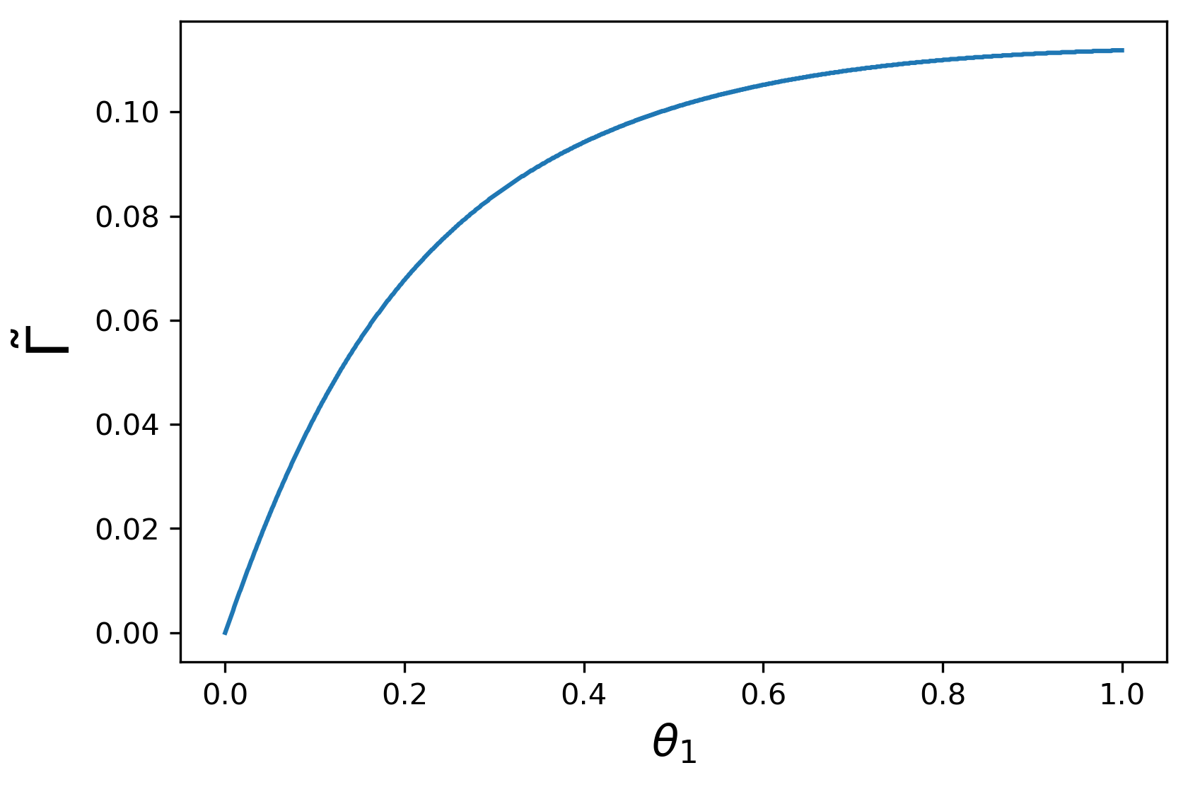
Figure 1: Given $\theta_{1}\in(0,1]$ and $\theta_{\varepsilon}=0$, the critical $\tilde{\Gamma}(\theta_{1})$ for equilibrium existence.

In the following, we only consider cases with

$$\theta_{\varepsilon}\in[10^{-4},9],\ \text{i.e., }\frac{\sigma_{\varepsilon}}{\sigma_{2}}\in[10^{-2},3].$$

When $\theta_{\varepsilon}<10^{-4}$ or $\theta_{\varepsilon}>9$, the results seem to have no essential changes.

Strategies and profits of HFT and IT. To show the results more clearly, we divide them into three situations with respect to HFT’s different inventory-averse levels. For IT, the profit has a linear relationship with the action, i.e., $\mathbb{E}(\pi^{\text{IT}})=\frac{\sigma_{2}\sigma_{v}}{2}A,$ so we only show the results for profit.

(1) HFT is light inventory averse $\bm{(\Gamma\in[0,1]).}$ Figure 2 presents the direction of HFT’s order $x_{1}$: in period 1, HFT always builds up positions in the same direction as IT.

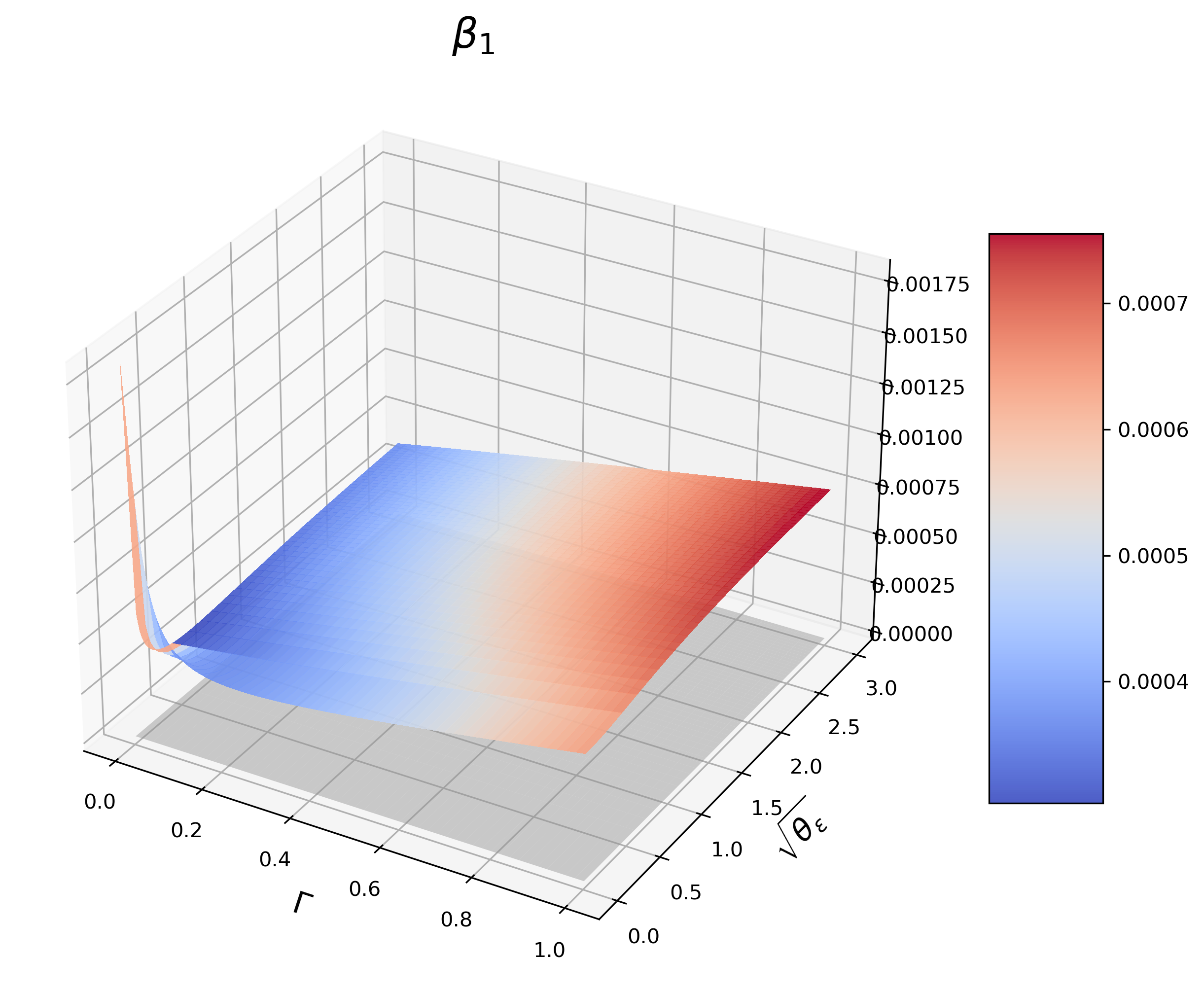
(a) $\theta_{1}=10^{-4}.$

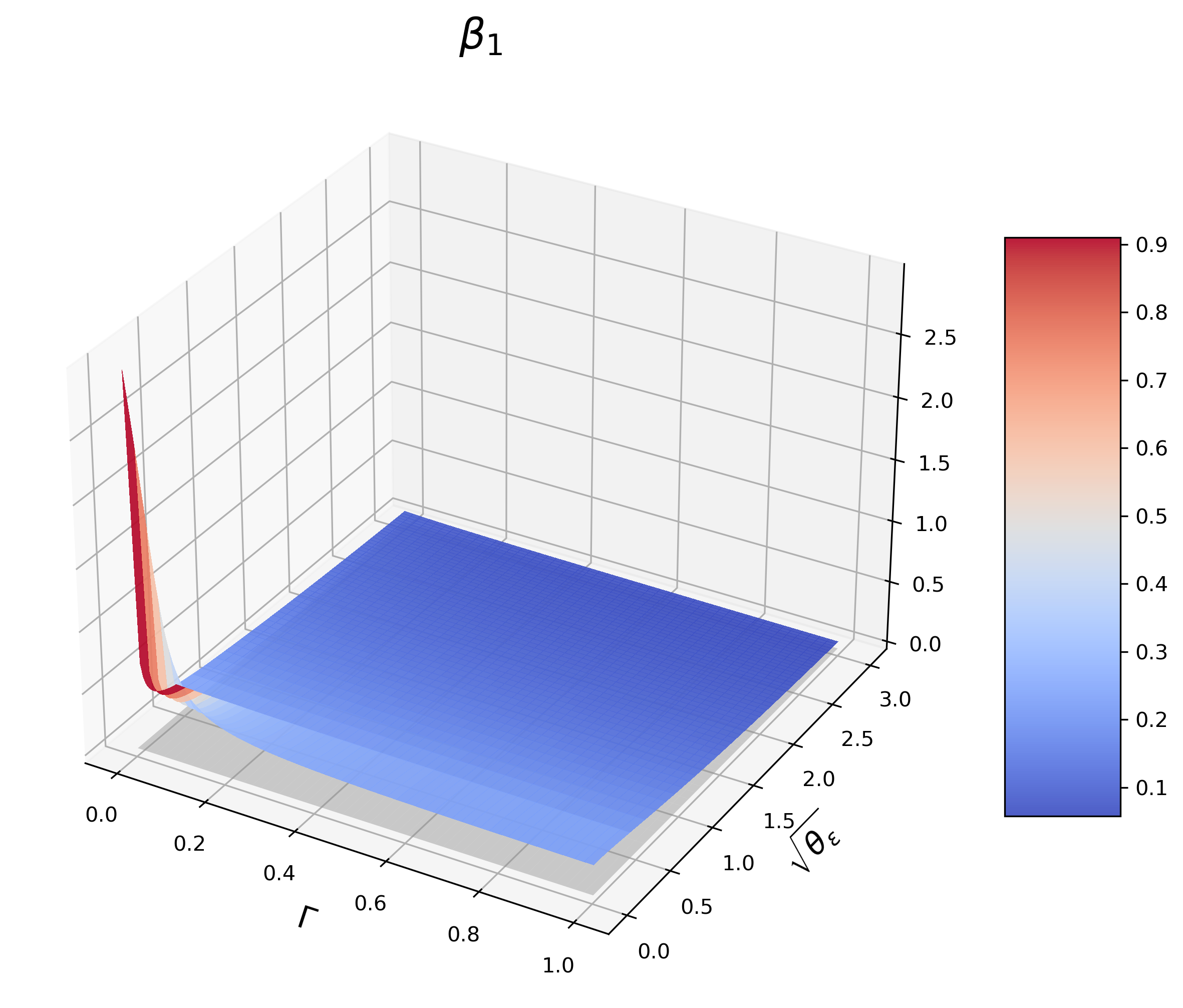
(b) $\theta_{1}=0.1.$

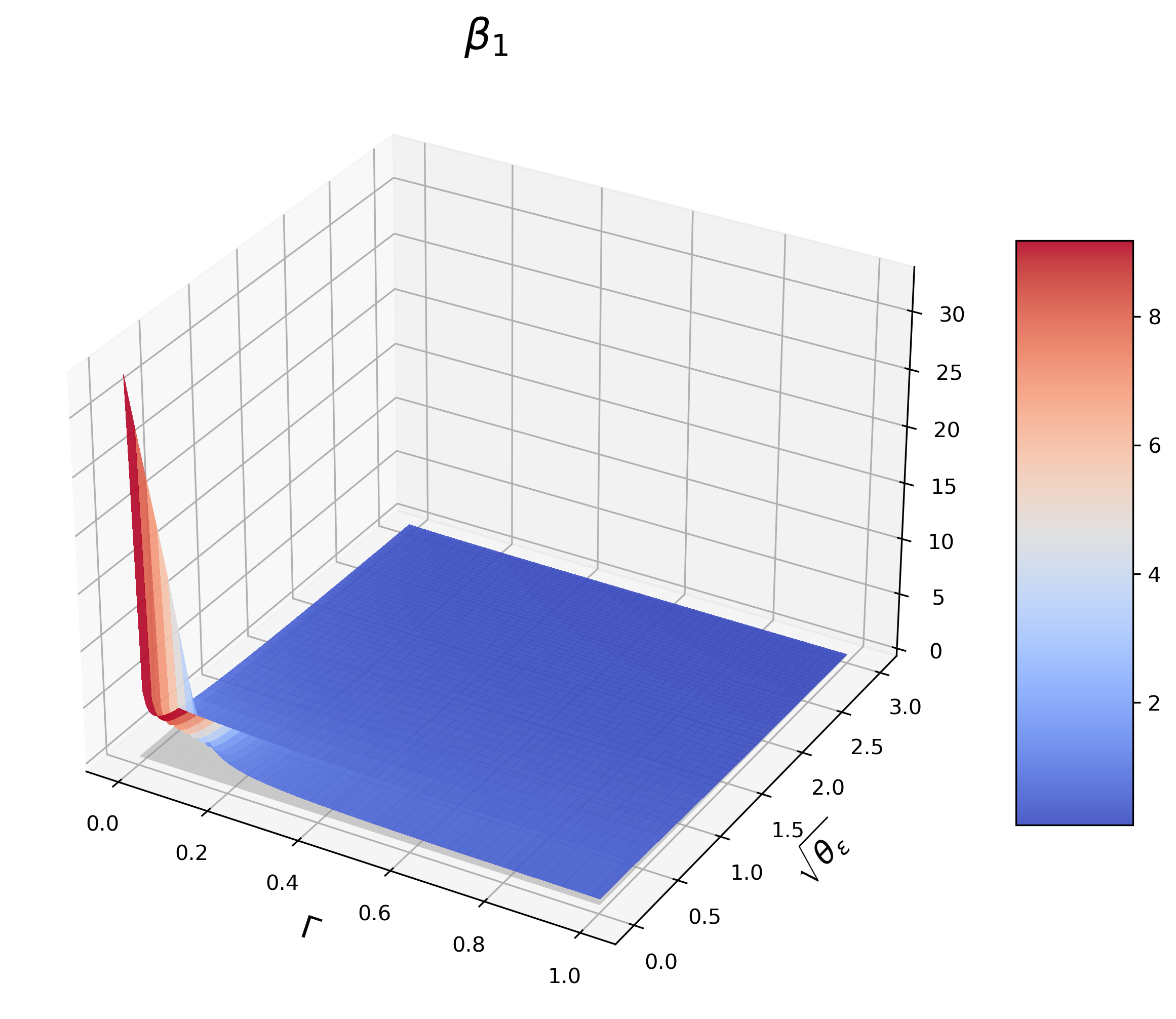
(c) $\theta_{1}=1.$

Figure 2: Direction of $x_{1},\Gamma\in[0,1]$. The grey plane refers to $\beta_{1}=0$,
which is the dividing plane of $x_{1}$’s direction.

(a) $\theta_{1}=10^{-4}.$

(b) $\theta_{1}=0.1.$

(c) $\theta_{1}=1.$

Figure 3: Direction of $x_{2},\Gamma\in[0,1]$. The grey plane refers to $\beta_{21}+\beta_{23}\beta_{1}=0$,
which is the dividing plane of $x_{2}$’s direction.

The direction of $x_{2}$ is shown in Figure 3. When the colored surface falls below the grey plane, HFT front-runs, otherwise, she acts as a small IT. As can be seen from (b) and (c), if the inventory penalty $\Gamma$ is mild, HFT acts as a small IT. Otherwise, HFT acts as a front-runner when the signal is relatively vague. It also holds for $\theta_{1}=10^{-4}$, which will be illustrated later. It is because the signal vagueness makes HFT quite uncertain about $v$, so in period 2, she closes some positions to reduce inventory cost. Comparing (b) and (c), when $\theta_{1}$ is larger, HFT trades reversely for smaller $\Gamma$ and $\theta_{\varepsilon}$. Since larger the $\theta_{1},$ less the impact $x_{1}$ can cause, and larger the position she is able to establish, which puts her under greater inventory pressure. From (c), we further see that when $\Gamma$ grows to a certain extent, HFT acts as a front-runner even if the signal is perfect.

Figure 4 compares HFT’s holding and impact profit in (2), which indicates that the former has the upper hand. When acting as a small IT or a front-runner with less inventory aversion, HFT infers information about $v$ and bets on it, the profits are mainly from investments in the risky asset.

(a) $\theta_{1}=10^{-4}.$

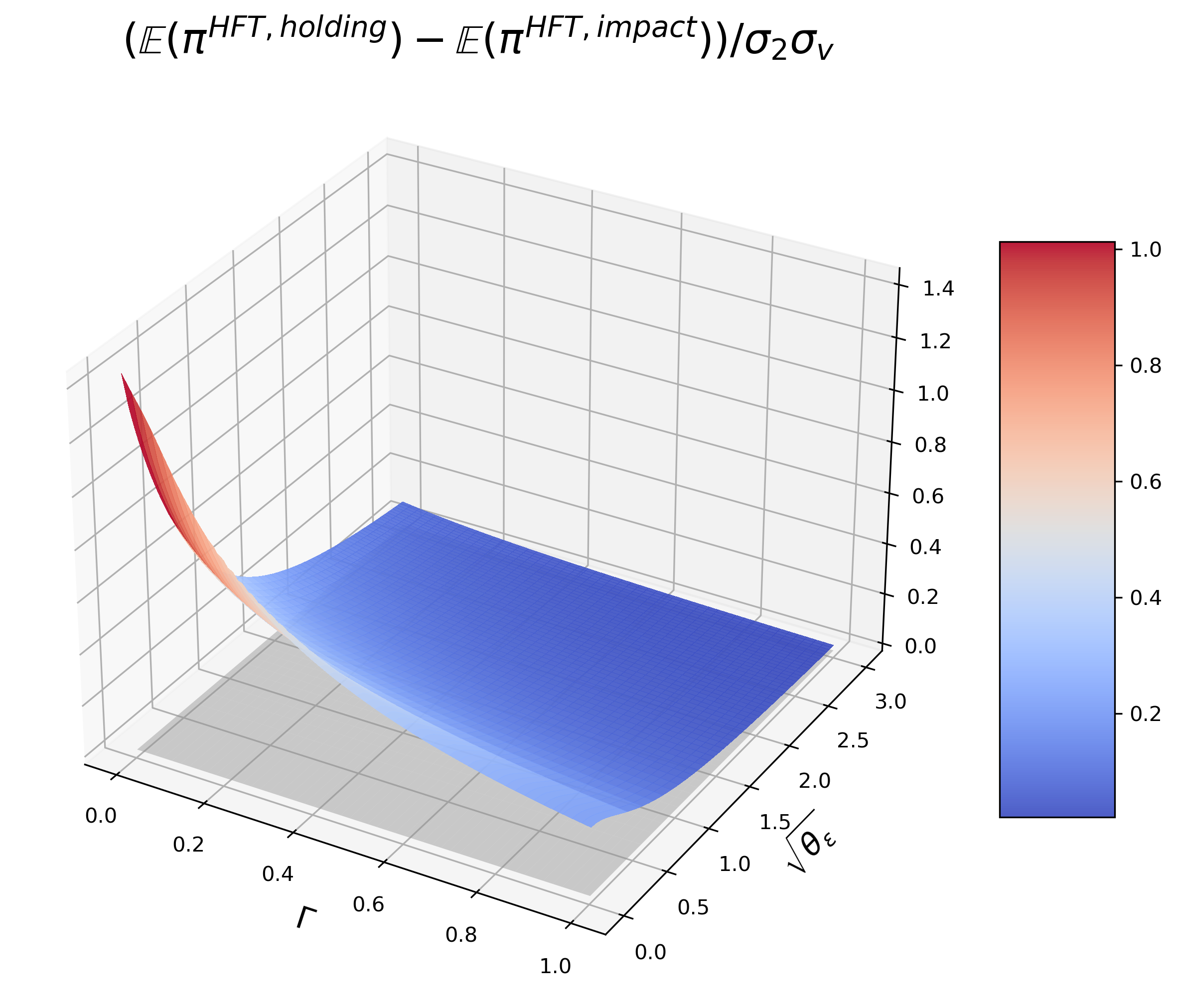
(b) $\theta_{1}=0.1.$

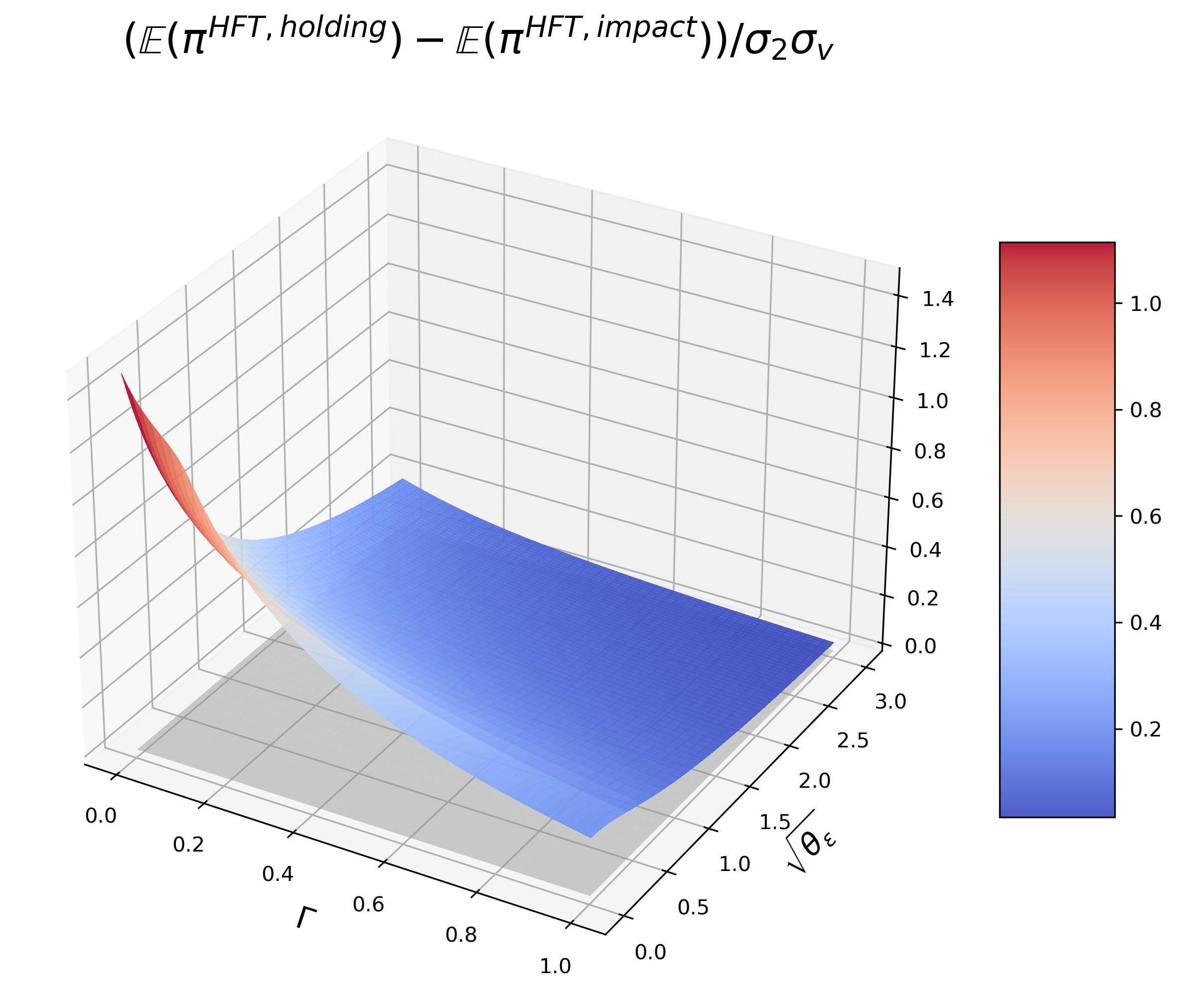
(c) $\theta_{1}=1.$

Figure 4: Comparation of HFT’s holding and impact profit, $\Gamma\in[0,1]$.
The grey plane refers to $\mathbb{E}(\pi^{\text{HFT,holding}})=\mathbb{E}(\pi^{\text{HFT,impact}})$.

HFT’s total profit is given in Figure 5. In general, it decreases with $\theta_{\varepsilon}$ and $\Gamma$. It is because a rough signal disables her to distinguish $v$ from $\hat{i}$ precisely, while the large inventory aversion prevents her from holding a large position, either of the above makes her trade more conservatively and receive fewer profits. Surprisingly, from (c), when $\theta_{1}$ is large and $\theta_{\varepsilon}$ is small, HFT’s profit first increases with $\Gamma$. Since for minor $\Gamma$s, HFT’s loss on signal inaccuracy drops rapidly as $\Gamma$ grows, which exceeds the decrease of investment income. When $\theta_{1}$ is small or $\theta_{\varepsilon}$ is large, the reduction in loss on signal noise is insignificant, as a result, HFT’s profit decreases.

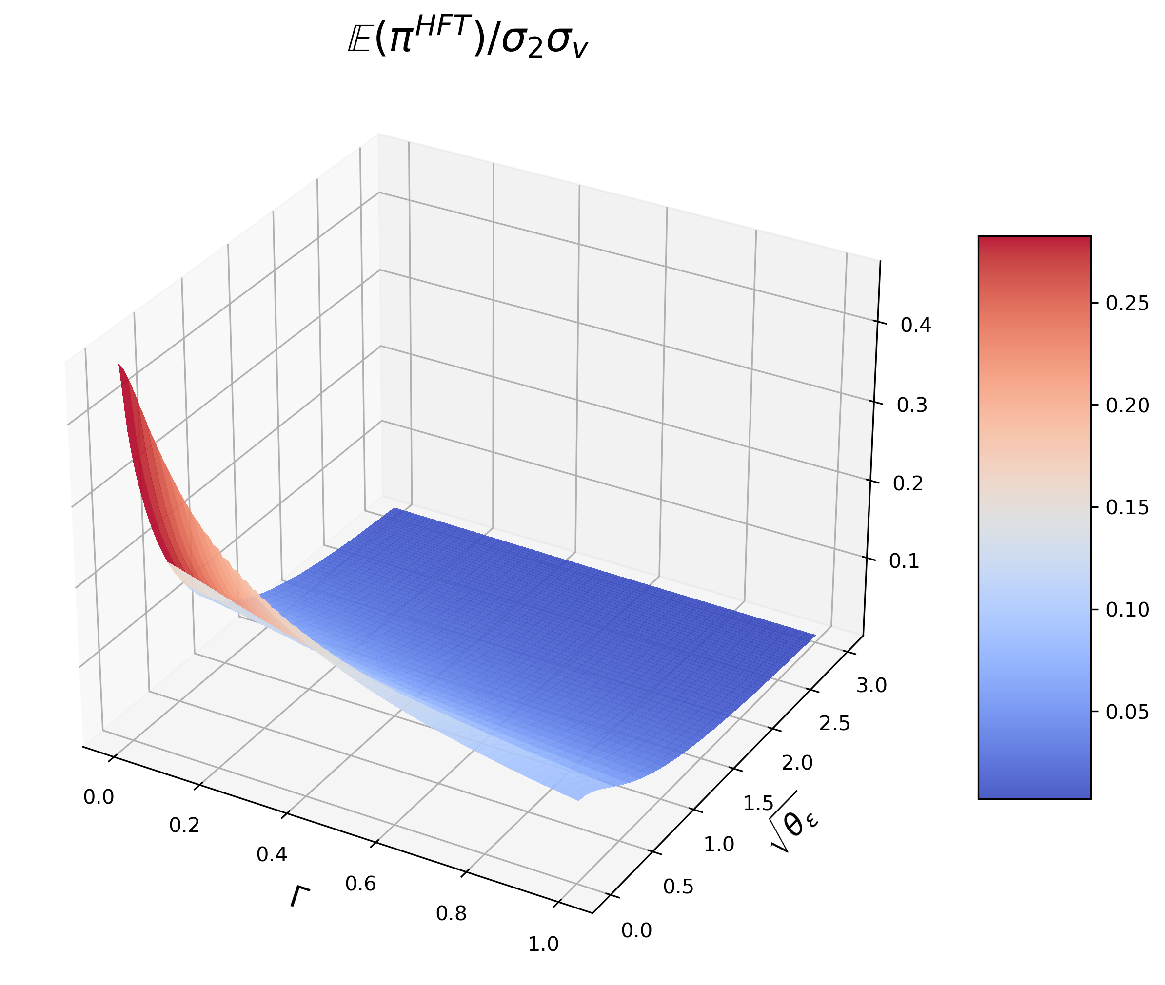
(a) $\theta_{1}=10^{-4}.$

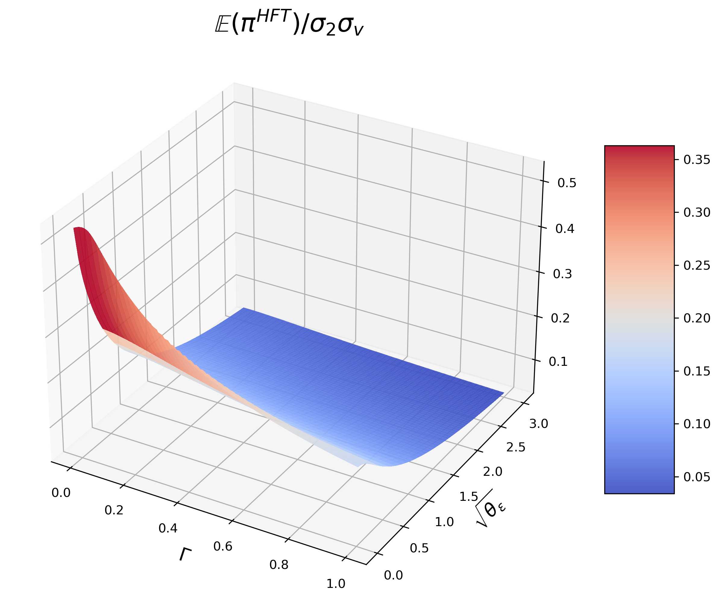
(b) $\theta_{1}=0.1.$

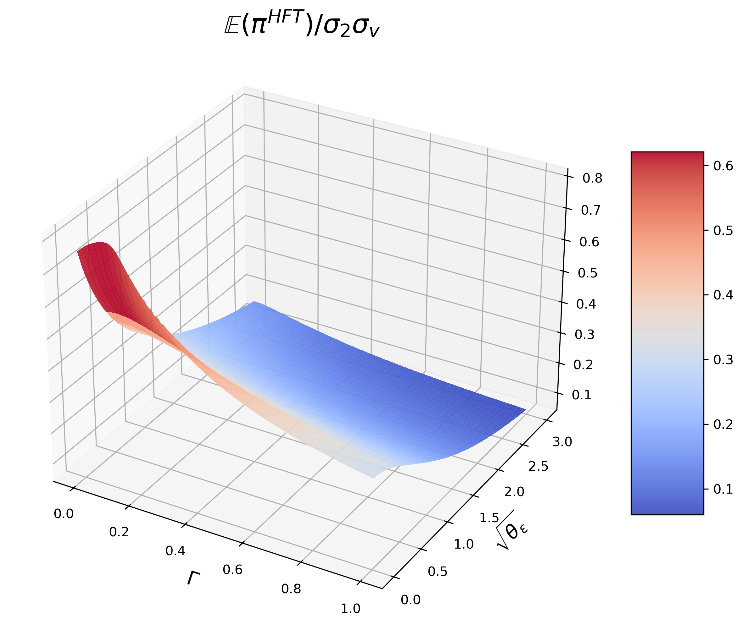
(c) $\theta_{1}=1.$

Figure 5: HFT’s profit, $\Gamma\in[0,1]$.

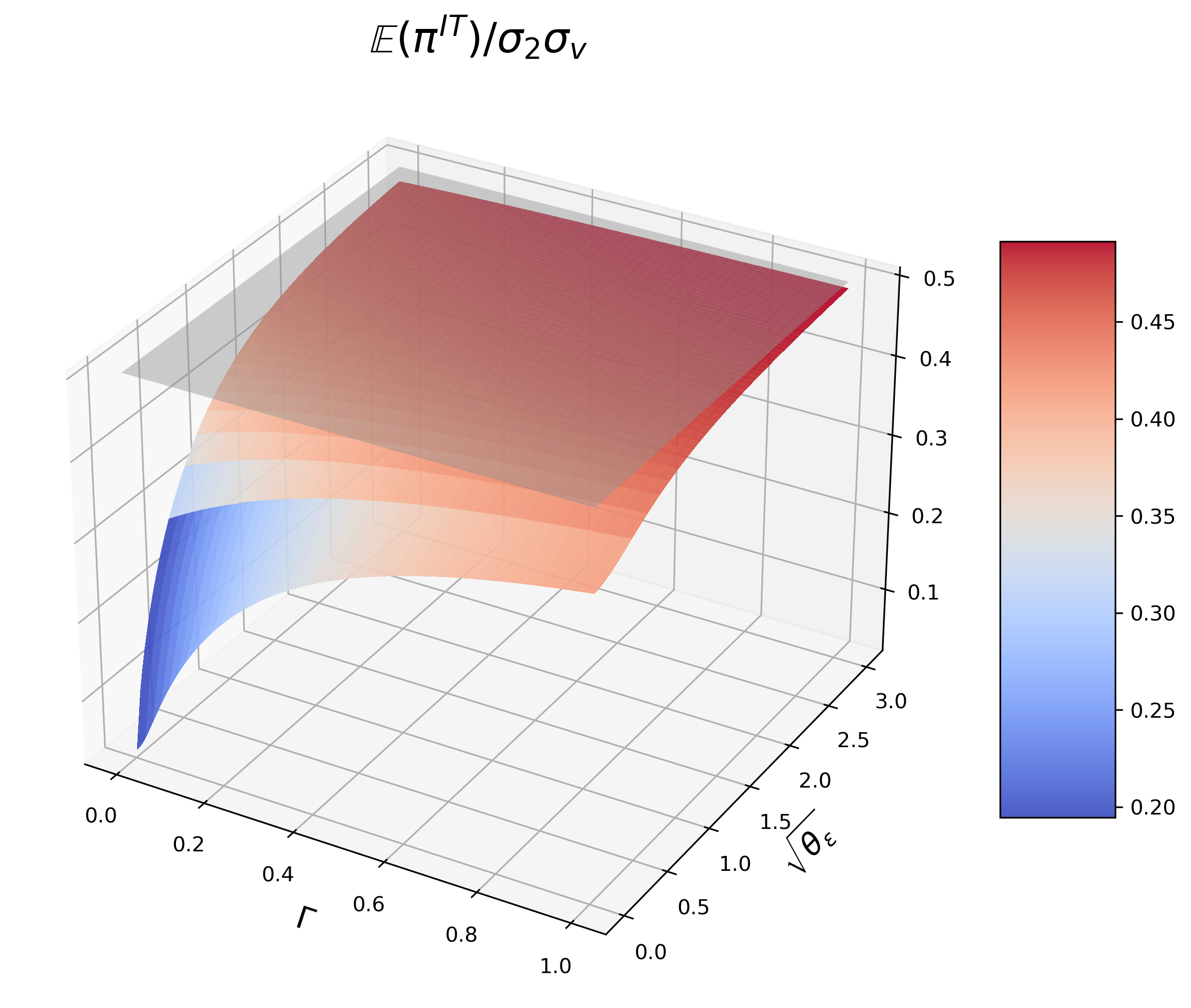
(a) $\theta_{1}=10^{-4}.$

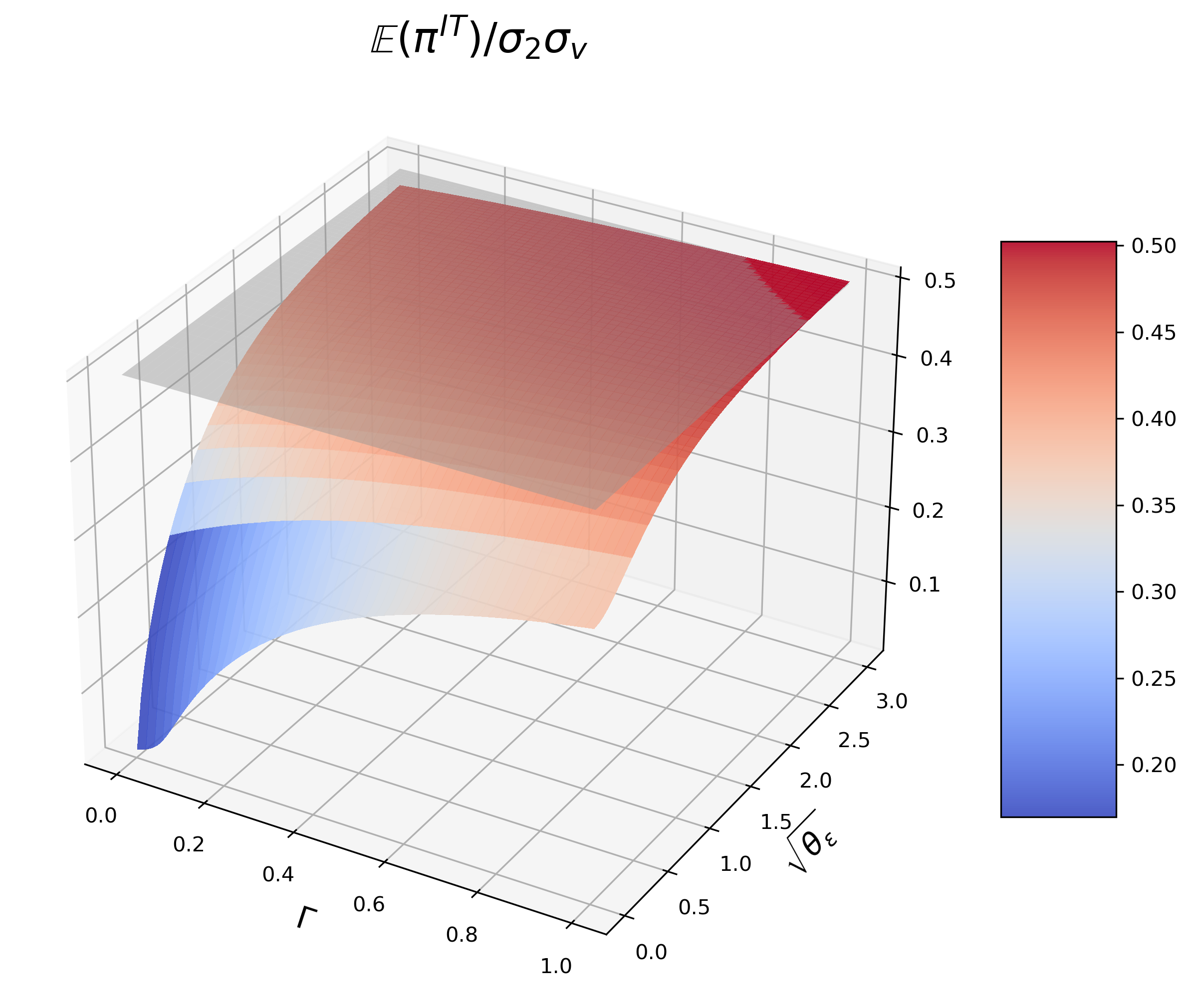
(b) $\theta_{1}=0.1.$

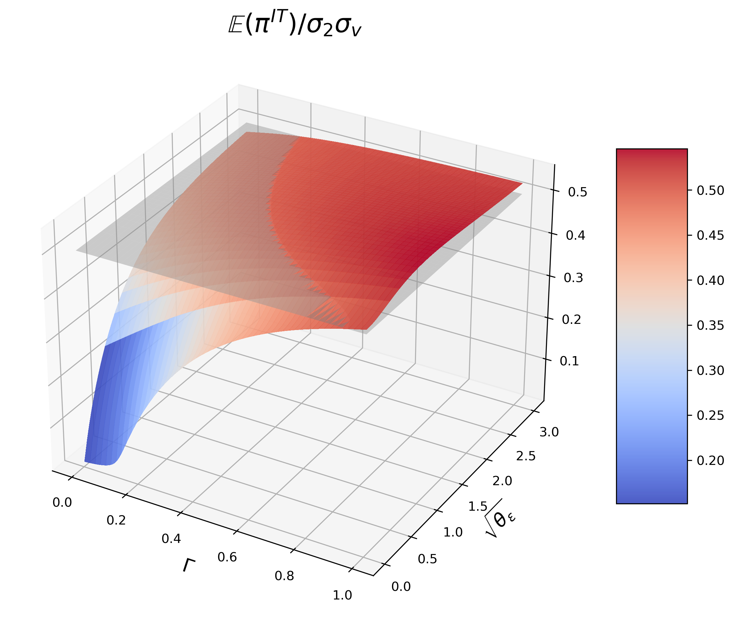
(c) $\theta_{1}=1.$

Figure 6: IT’s profit, $\Gamma\in[0,1]$. The grey plane refers to $\mathbb{E}(\pi^{\text{IT}})=\frac{\sigma_{2}\sigma_{v}}{2},$
which is IT’s profit without HFT.

Combining Figure 6 and Figure 3, IT is always worse off with a small IT, since the latter increases her price impact in both periods. When $\theta_{1}\geq 0.1,$ HFT benefits IT as $\Gamma$ and $\theta_{\varepsilon}$ grow to a certain extent (see (b) and (c) of Figure 6). In this case, HFT front-runs, the time-2 transaction cost she shares for IT exceeds the loss caused by her time-1 trades. When $\theta_{1}\in(0,0.1),$ it is also true but needs larger $\Gamma$ and $\theta_{\varepsilon}.$ Given $\theta_{1}$ and $\Gamma$, in the area where HFT harms IT, IT’s profit always increases with $\theta_{\varepsilon}$, since the signal noise protects IT from being precisely detected.

Comparing IT’s profits with different $\theta_{1},$ we find that the phenomenon of HFT benefiting IT is more likely to appear for larger $\theta_{1}$. On the one hand, a larger $\theta_{1}$ leads HFT to take front-running strategy in more cases. On the other hand, more time-1 noise trading decreases $x_{1}$’s adverse impact. Both of the above are advantageous to IT. Given $\theta_{1}$ and $\theta_{\varepsilon},$ HFT’s final position decreases with $\Gamma$, either from less same-direction trading or from more opposite-direction trading, which implies a greater likelihood of HFT benefiting IT. To sum up, there is a critical value of $\theta_{\varepsilon}$, with which HFT benefits IT, and this critical value decreases with $\theta_{1}$ and $\Gamma$.

(2) HFT is medium inventory averse $\bm{(\Gamma\in[1,20]).}$ Relying on the speed advantage, HFT still trades in the same direction as IT at $t=1$ (see Figure 7). Comparing (a) of Figure 3 and 8, when HFT is more inventory averse, she is more likely to provide liquidity back at $t=2$.

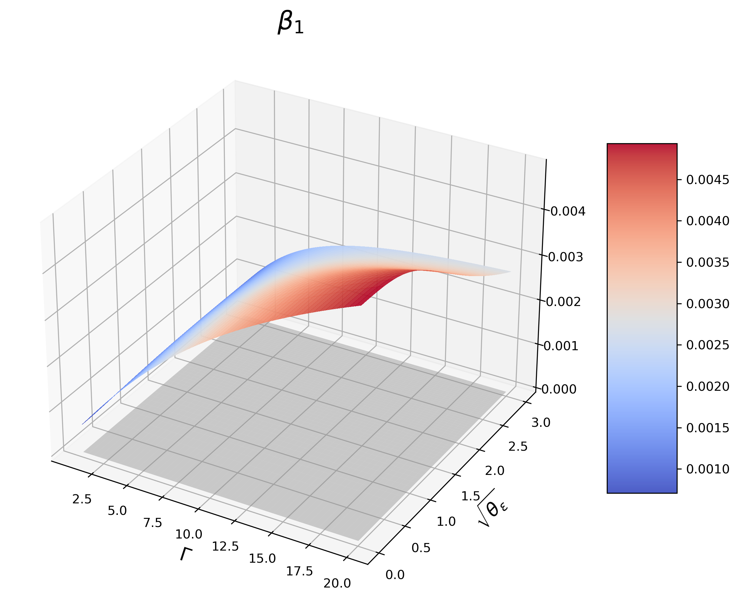
(a) $\theta_{1}=10^{-4}.$

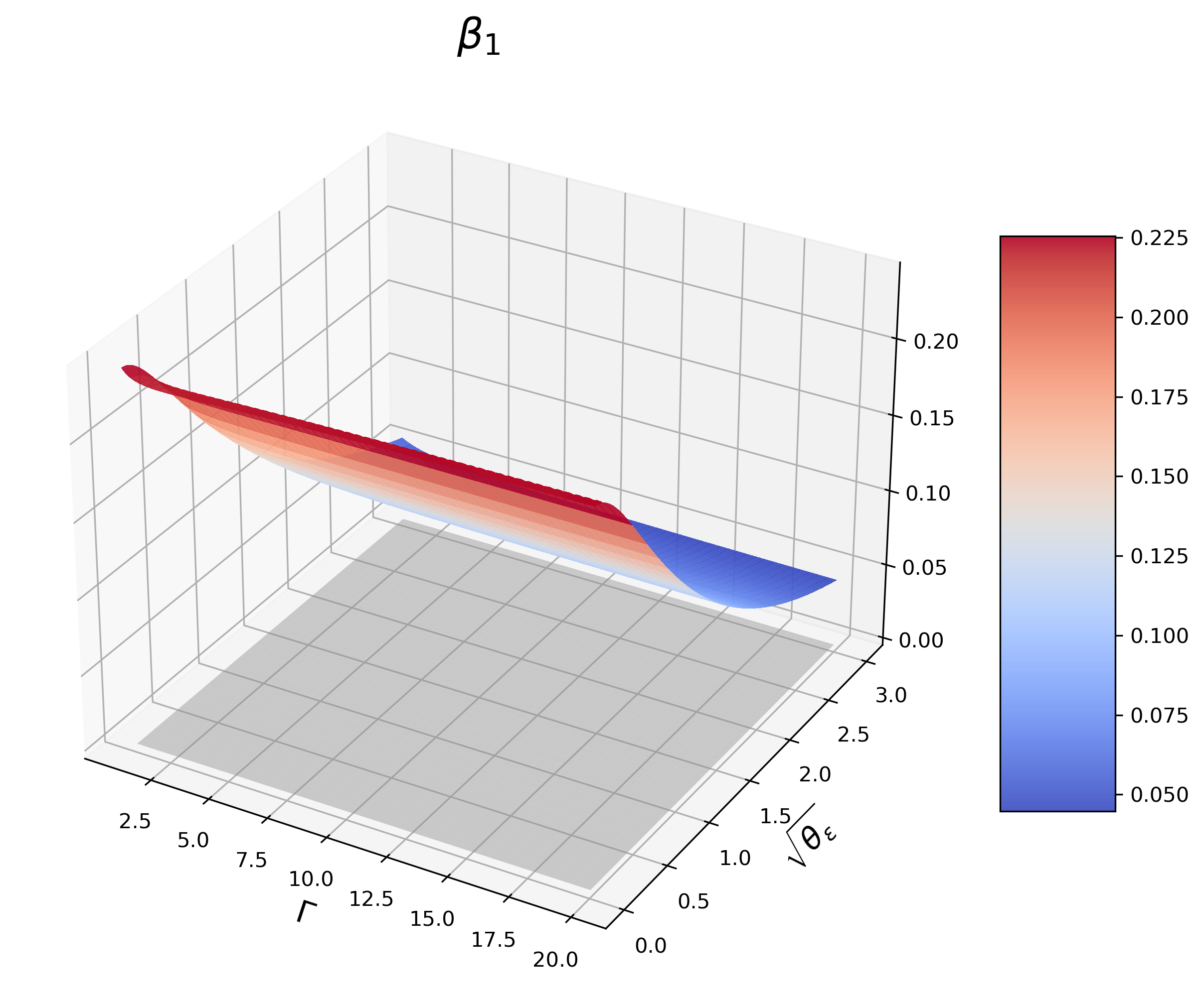
(b) $\theta_{1}=0.1.$

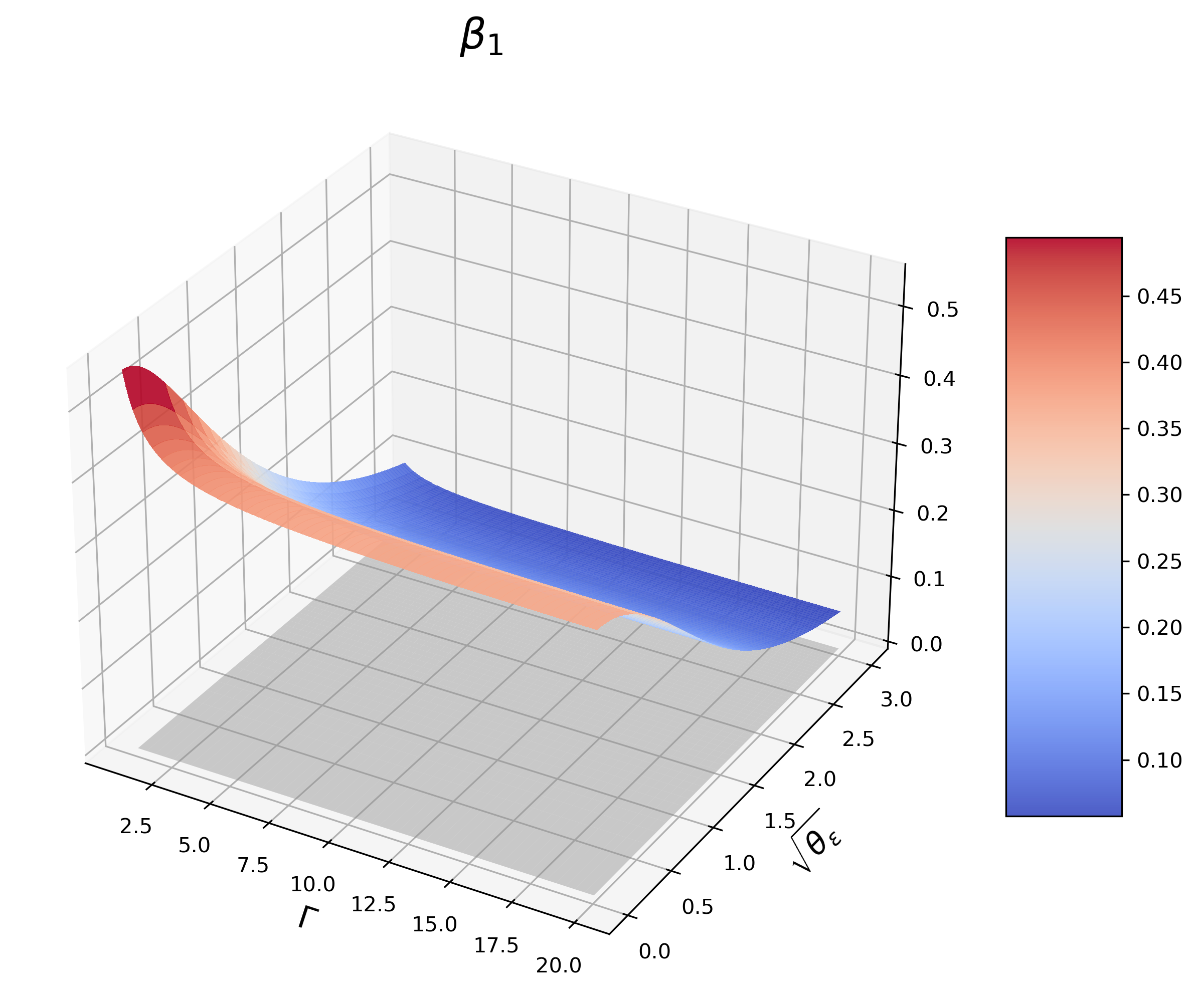
(c) $\theta_{1}=1.$

Figure 7: Direction of $x_{1},\Gamma\in[1,20]$. The grey plane refers to $\beta_{1}=0$,
which is the dividing plane of $x_{1}$’s direction.

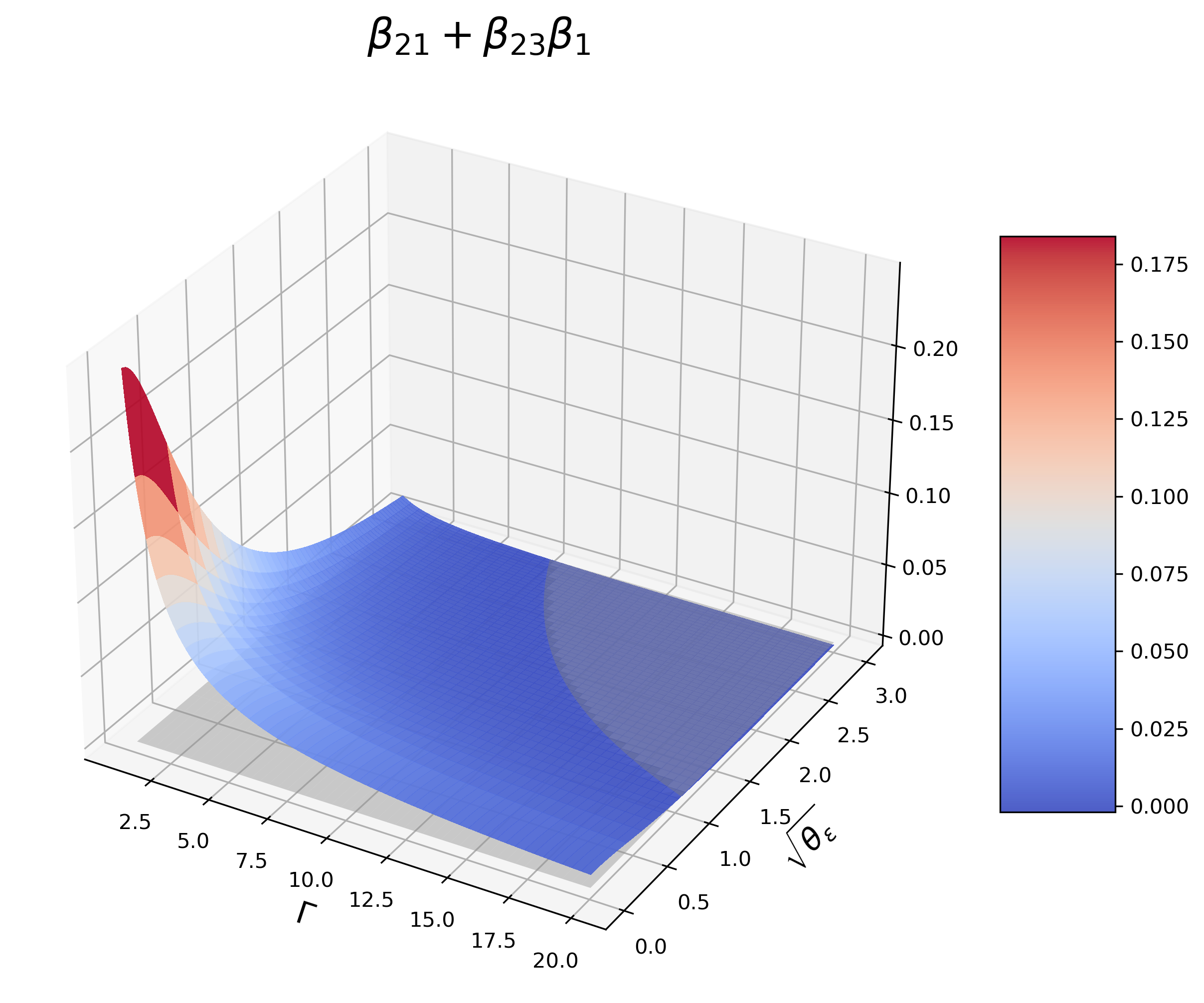
(a) $\theta_{1}=10^{-4}.$

(b) $\theta_{1}=0.1.$

(c) $\theta_{1}=1.$

Figure 8: Direction of $x_{2},\Gamma\in[1,20]$. The grey plane refers to $\beta_{21}+\beta_{23}\beta_{1}=0$,
which is the dividing plane of $x_{2}$’s direction.

The origin of HFT’s profit is further analyzed through Figure 9. In (b) and (c), front-runners with high inventory aversion no longer bets on $v$, their profits mainly come from the price impact caused by IT’s order. It also holds for $\theta_{1}=10^{-4},$ which needs very large $\Gamma$s. HFT’s total profit is given in Figure 10, it still decreases with $\Gamma$ and $\theta_{\varepsilon}$.

(a) $\theta_{1}=10^{-4}.$

(b) $\theta_{1}=0.1.$

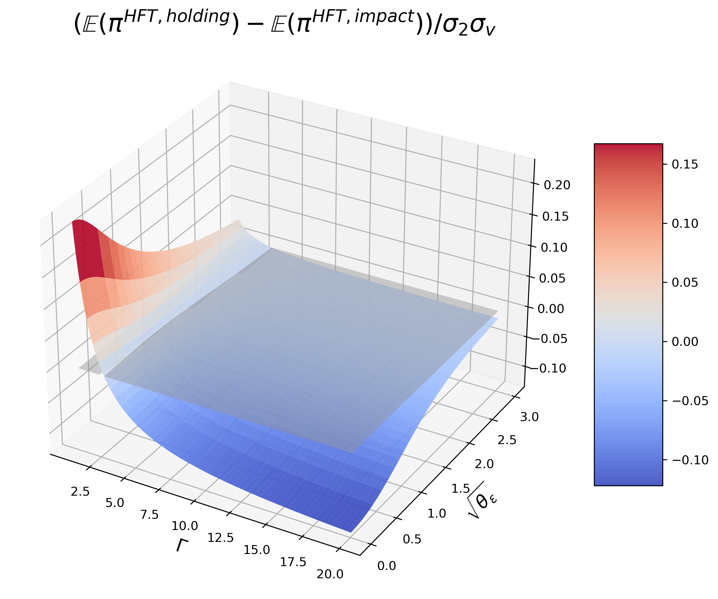
(c) $\theta_{1}=1.$

Figure 9: Comparation of HFT’s holding and impact profit, $\Gamma\in[1,20]$.
The grey plane refers to $\mathbb{E}(\pi^{\text{HFT,holding}})=\mathbb{E}(\pi^{\text{HFT,impact}})$.

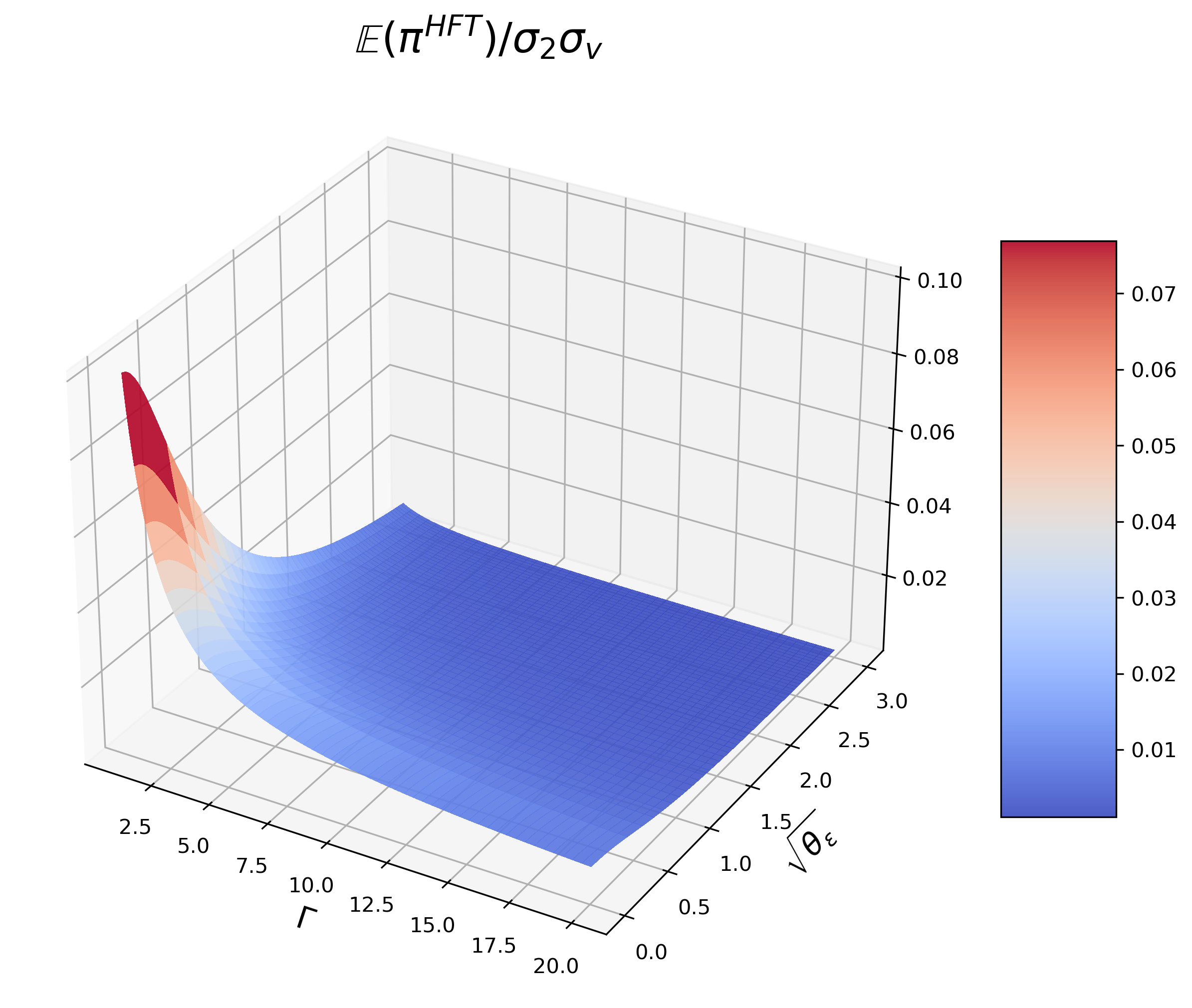
(a) $\theta_{1}=10^{-4}.$

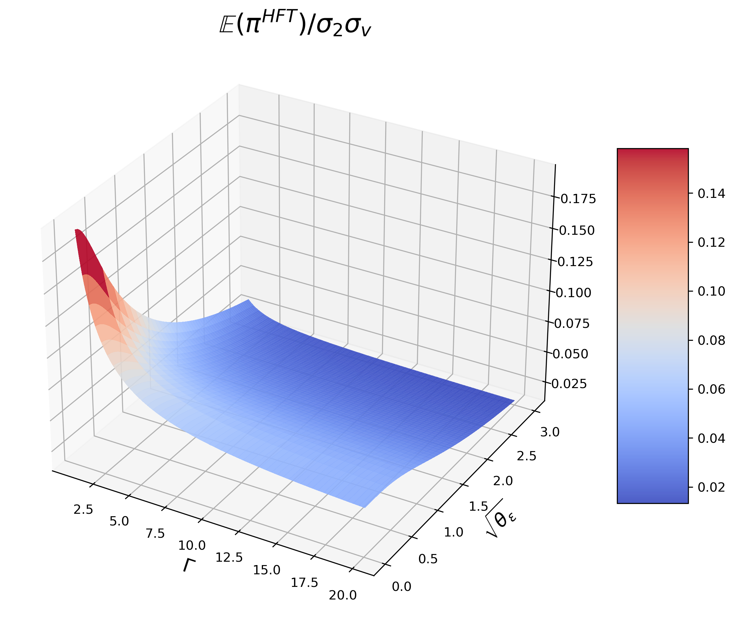
(b) $\theta_{1}=0.1.$

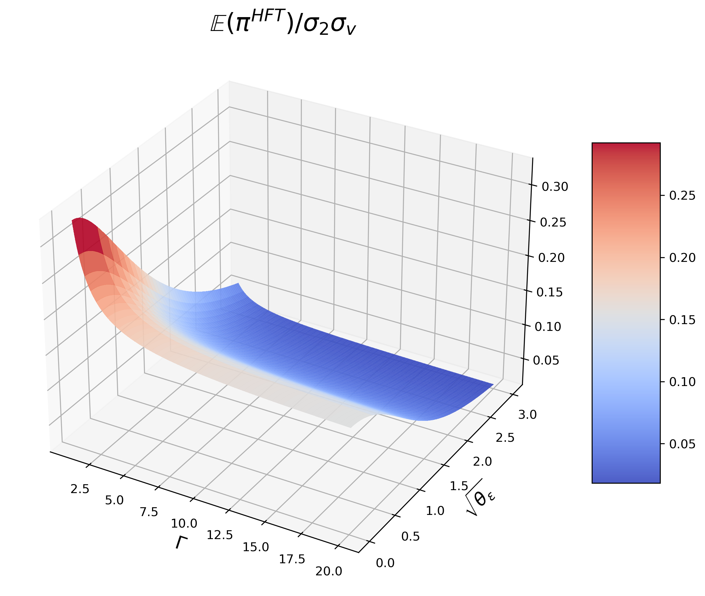
(c) $\theta_{1}=1.$

Figure 10: HFT’s profit, $\Gamma\in[1,20]$.

As shown in (b) and (c) of Figure 11, IT can still be benefited by the front-running HFT. Surprisingly, in this case, as indicated by (c), her profit may decrease with $\theta_{\varepsilon}$. The reason is: given $\theta_{1}$ and $\Gamma$, when the signal noise increases to a certain extent, HFT is unwilling to establish large positions at $t=1$ (see (c) of Figure 7), and there is no need for her to liquidate large positions at $t=2$ (see (c) of Figure 8), which makes her share less impact for IT, consequently, IT’s profit starts to decrease. Actually, this holds for any $\theta_{1}\in(0,1],$ but is more possible to happen for larger $\theta_{1}$, because if market noise has already provided enough shelter for IT, more signal noise may backfire. However, although IT’s profit is declining, it stays higher than that without the front-runner.

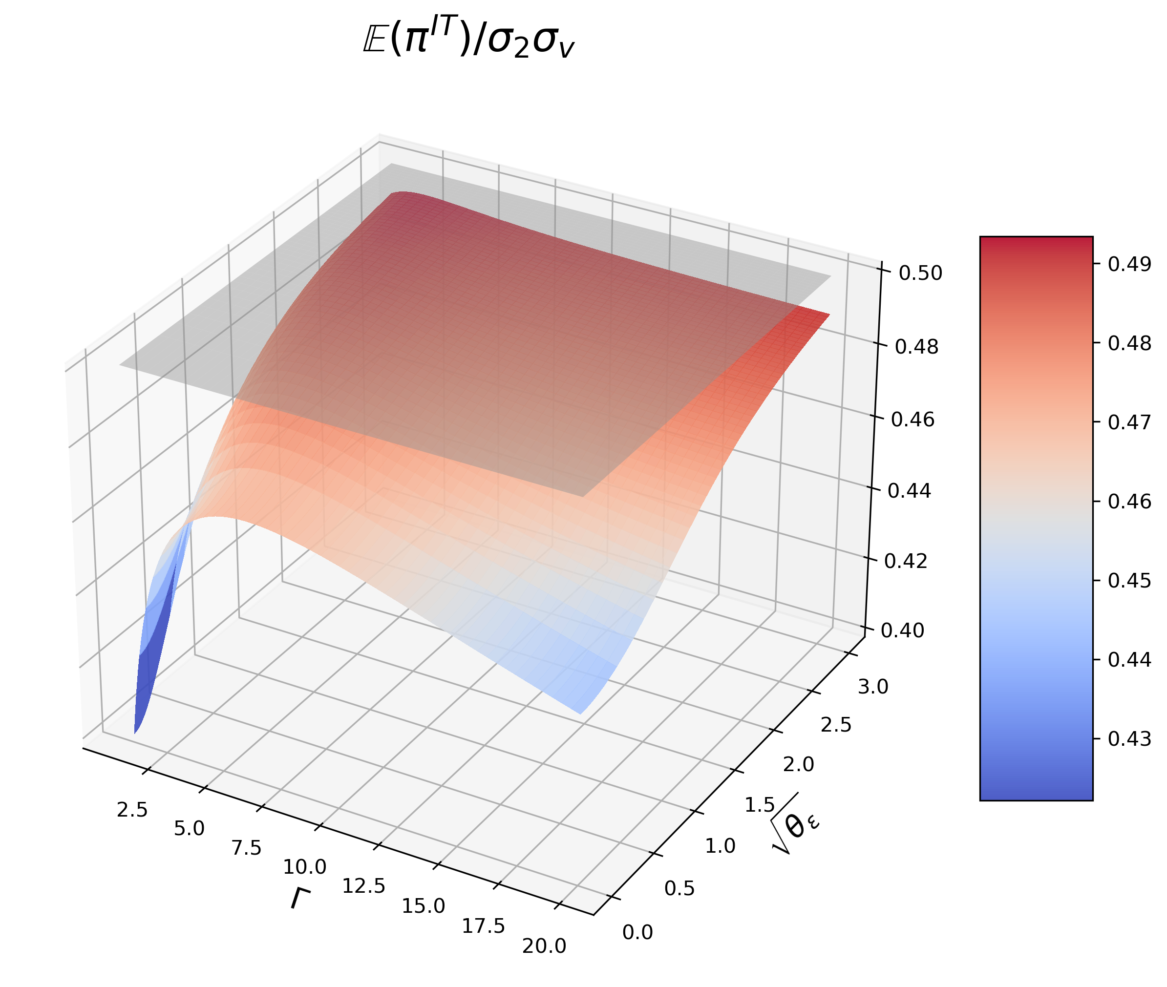
(a) $\theta_{1}=10^{-4}.$

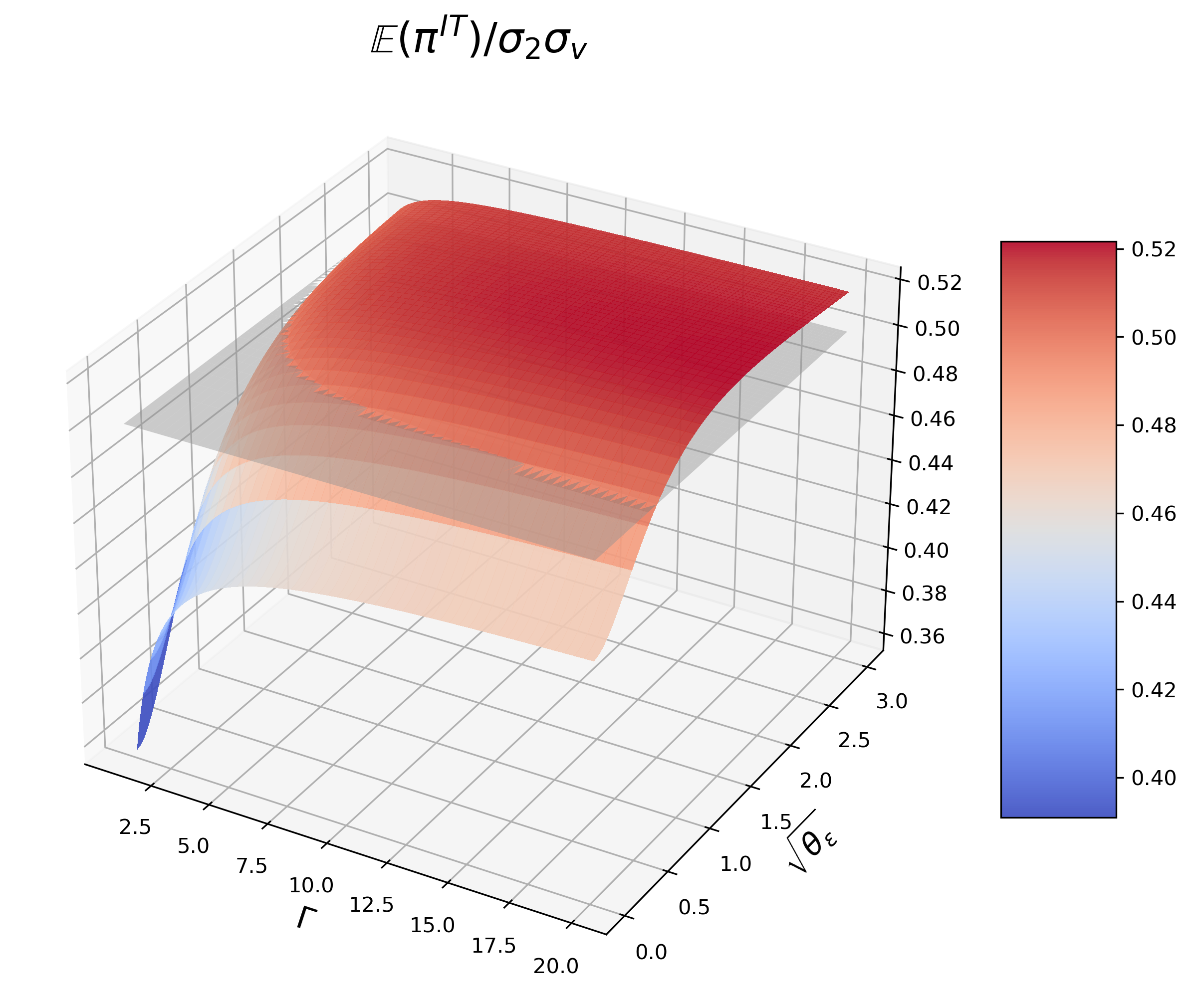
(b) $\theta_{1}=0.1.$

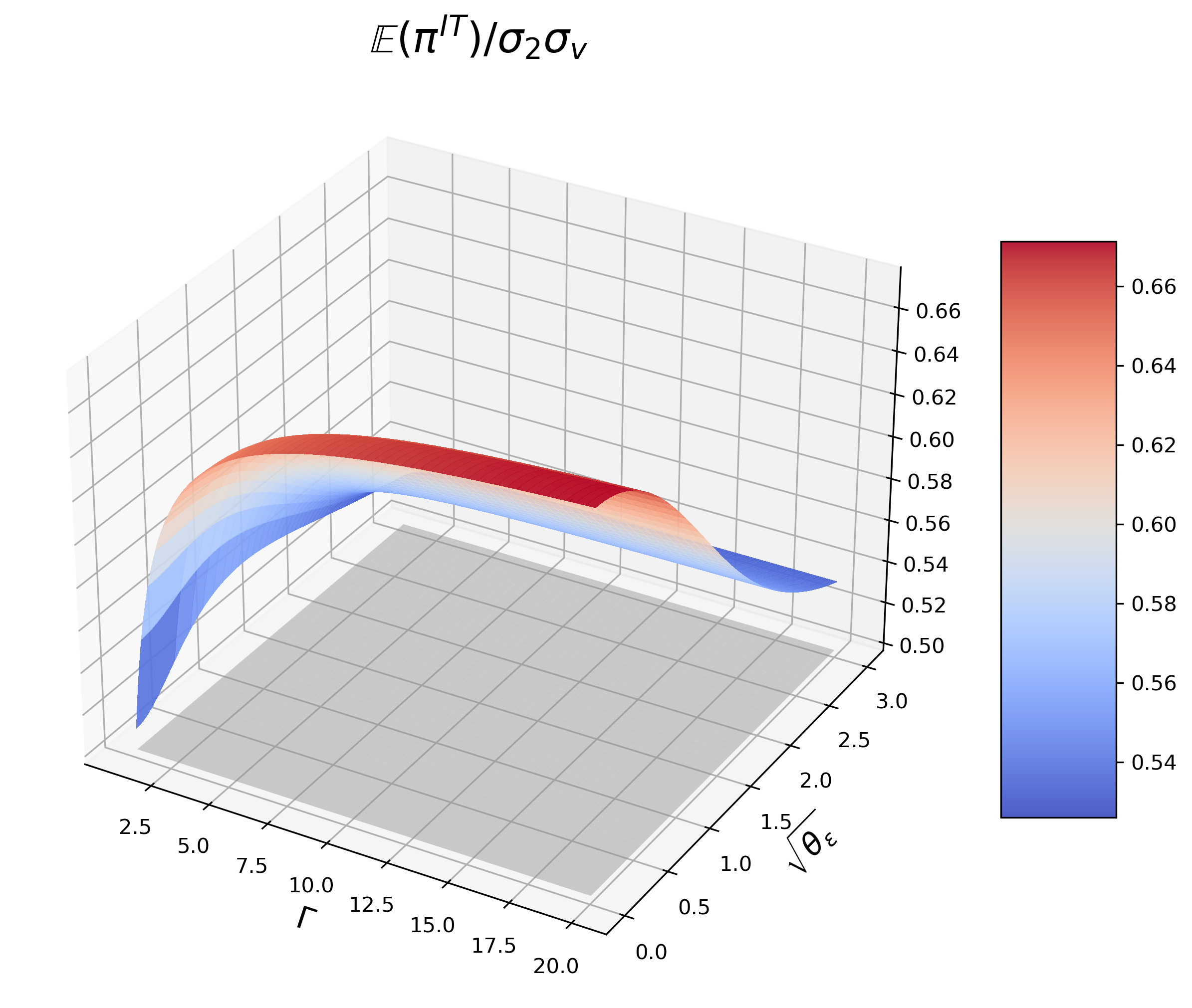
(c) $\theta_{1}=1.$

Figure 11: IT’s profit, $\Gamma\in[1,20]$. The grey plane refers to $\mathbb{E}(\pi^{\text{IT}})=\frac{\sigma_{2}\sigma_{v}}{2},$
which is IT’s profit without HFT.

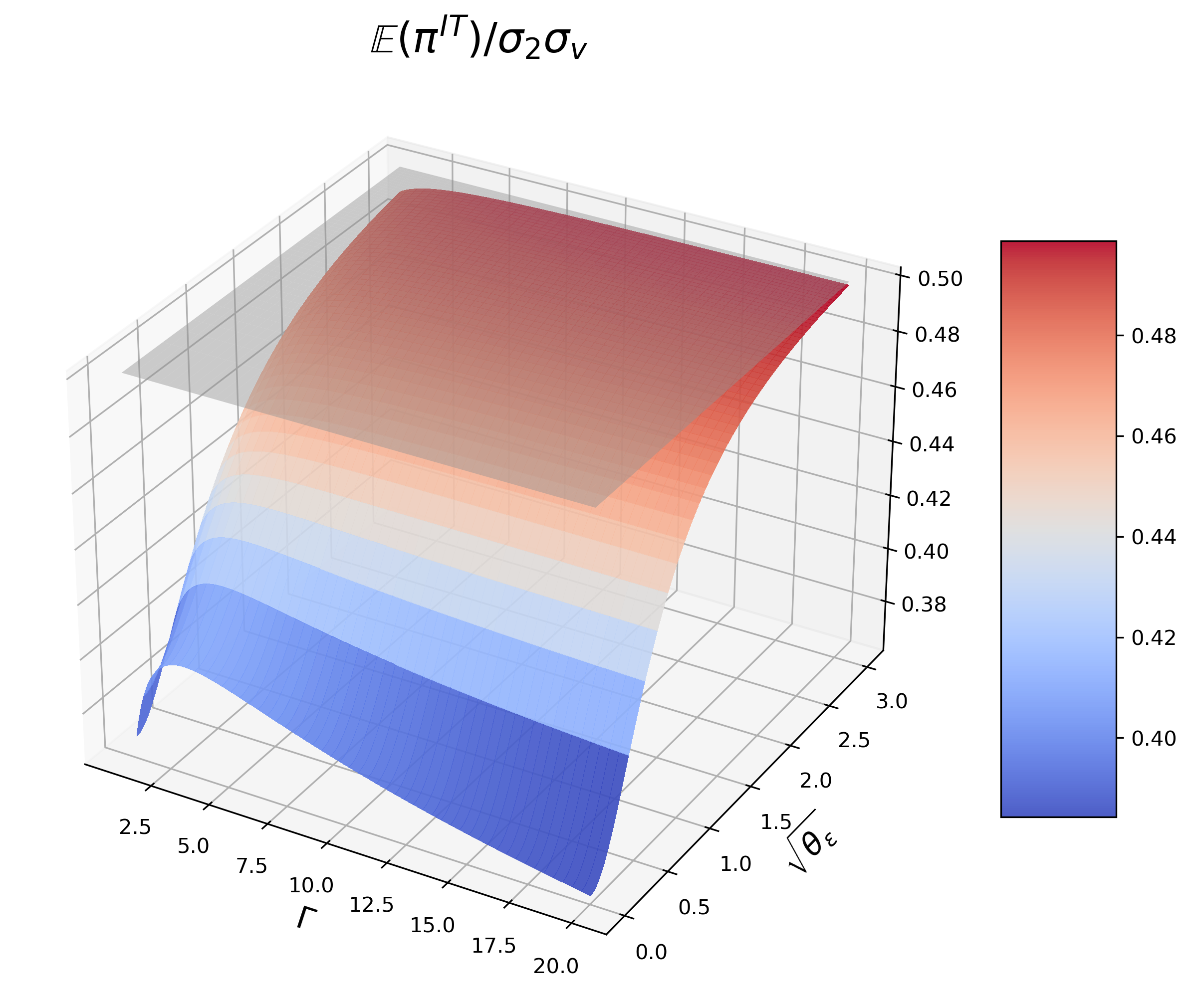
(a) IT’s profit.

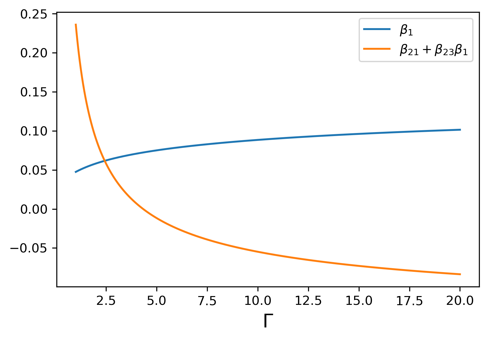
(b) HFT’s directions, $\theta_{\varepsilon}=10^{-4}.$

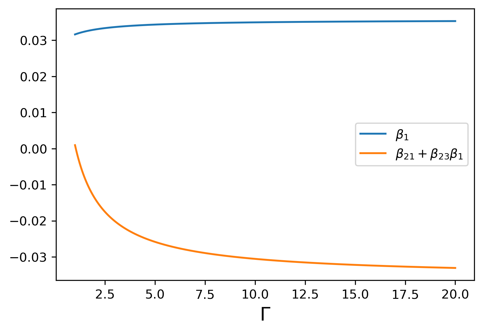
(c) HFT’s directions, $\theta_{\varepsilon}=4.$

Figure 12: $\theta_{1}=0.01$, IT’s profit and HFT’s trading directions.

Another noteworthy phenomenon is that given $\theta_{1}\in(0,0.07266)$, when HFT’s signal is not overly noisy, IT’s profit could decrease with $\Gamma$, which is not quite in line with common sense because a larger $\Gamma$ should deter HFT from establishing a large position to anticipate IT’s trading. In order to explain this pattern, we take $\theta_{1}=0.01$ as an example (in Figure 12). When $\theta_{\varepsilon}\leq 1.0531,$ IT’s profit indeed follows the increase-decrease pattern, as shown in (a). From (b) and (c), when $\Gamma$ is relatively small, $x_{2}$ declines sharply in both figures, which causes less impact, so IT’s profit increases. When $\Gamma$ is relatively large, for (c), since $\theta_{\varepsilon}=4,$ HFT is unsure about $v$, the increase of $x_{1}$ is always slower than the decrease of $x_{2}$, IT’s profit keeps increasing. However, in (b), both $x_{1}$ and $x_{2}$ change steadily. Since there is little noise trading during period 1, the increase of $x_{1}$ brings larger adverse impact for IT, and IT’s profit decreases.

We may wonder what kind of role HFT is playing when IT’s profit attains its maximum. We find surprisingly that when the time-1 market noise is small and HFT’s signal is relatively accurate, for example, (1) $\theta_{1}=10^{-4},\theta_{\varepsilon}\leq 9$; (2) $\theta_{1}=0.01,\theta_{\varepsilon}\leq 0.2,$ IT’s profit is maximal when HFT is a small IT. In other words, when HFT harms IT, in some extreme cases, she may harm IT more when she is a front-runner than she is a small IT. At the first glance, it contradicts with the finding of Roşu (2019) [19] that investors are better-off with a sufficiently inventory-averse fast trader. This is because [19] compares a specific small IT ($\Gamma=0$) with a specific front-runner ($\Gamma$ is sufficiently large), but we compare the small IT who harms IT least with all front-runners.

(3) HFT is extremely inventory averse $\bm{(\Gamma>20).}$ For extremely large $\Gamma$, most results remain the same as in the former case, except for HFT’s profit: when there is little high-speed noise trading, HFT may make more profits with a less accurate signal, as shown in (a) of Figure 13. It is because HFT’s profit is mainly decided by her intensity and the impact caused by IT, when $\theta_{1}$ is relatively small, HFT trades more conservatively but IT may trade more aggressively as $\theta_{\varepsilon}$ grows. When both $\theta_{1}$ and $\theta_{\varepsilon}$ are small, the latter dominates the former, so HFT’s profit increases; when $\theta_{1}$ or $\theta_{\varepsilon}$ is large, the opposite is true.

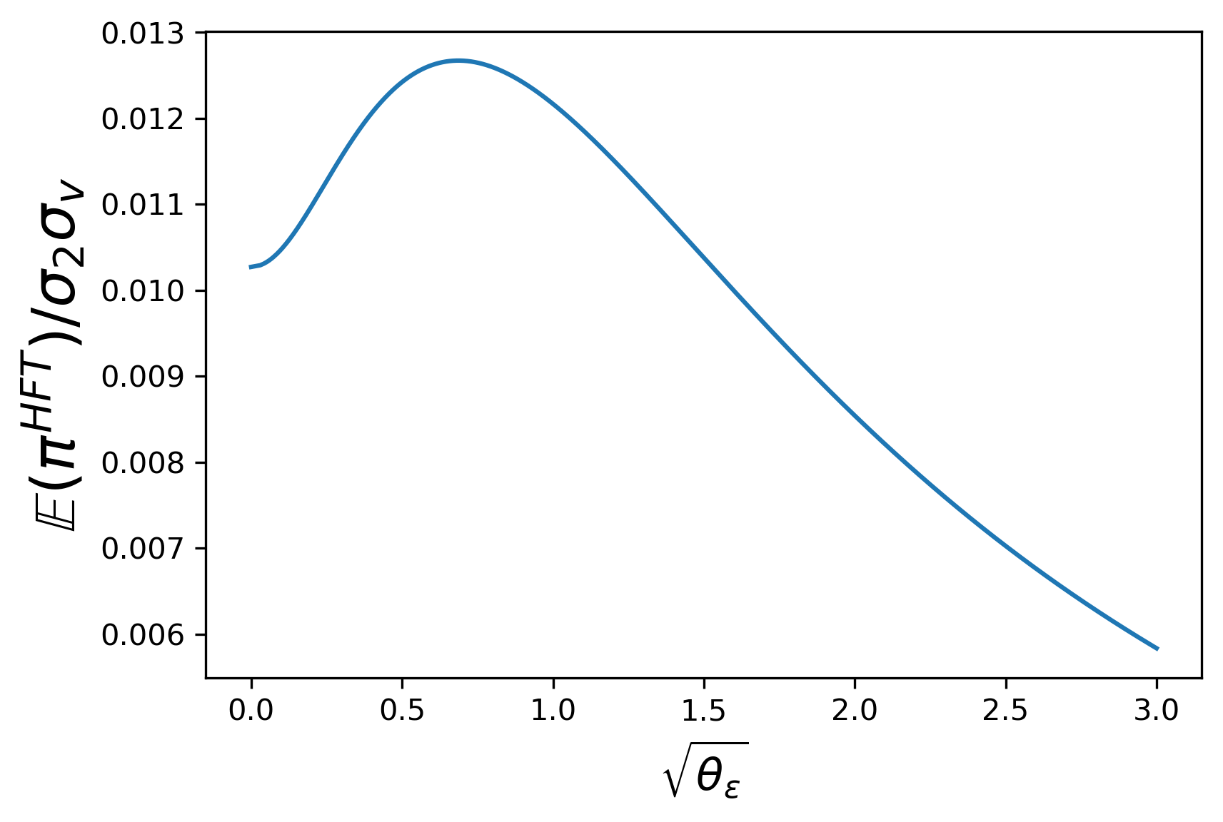
(a) HFT’s profit.

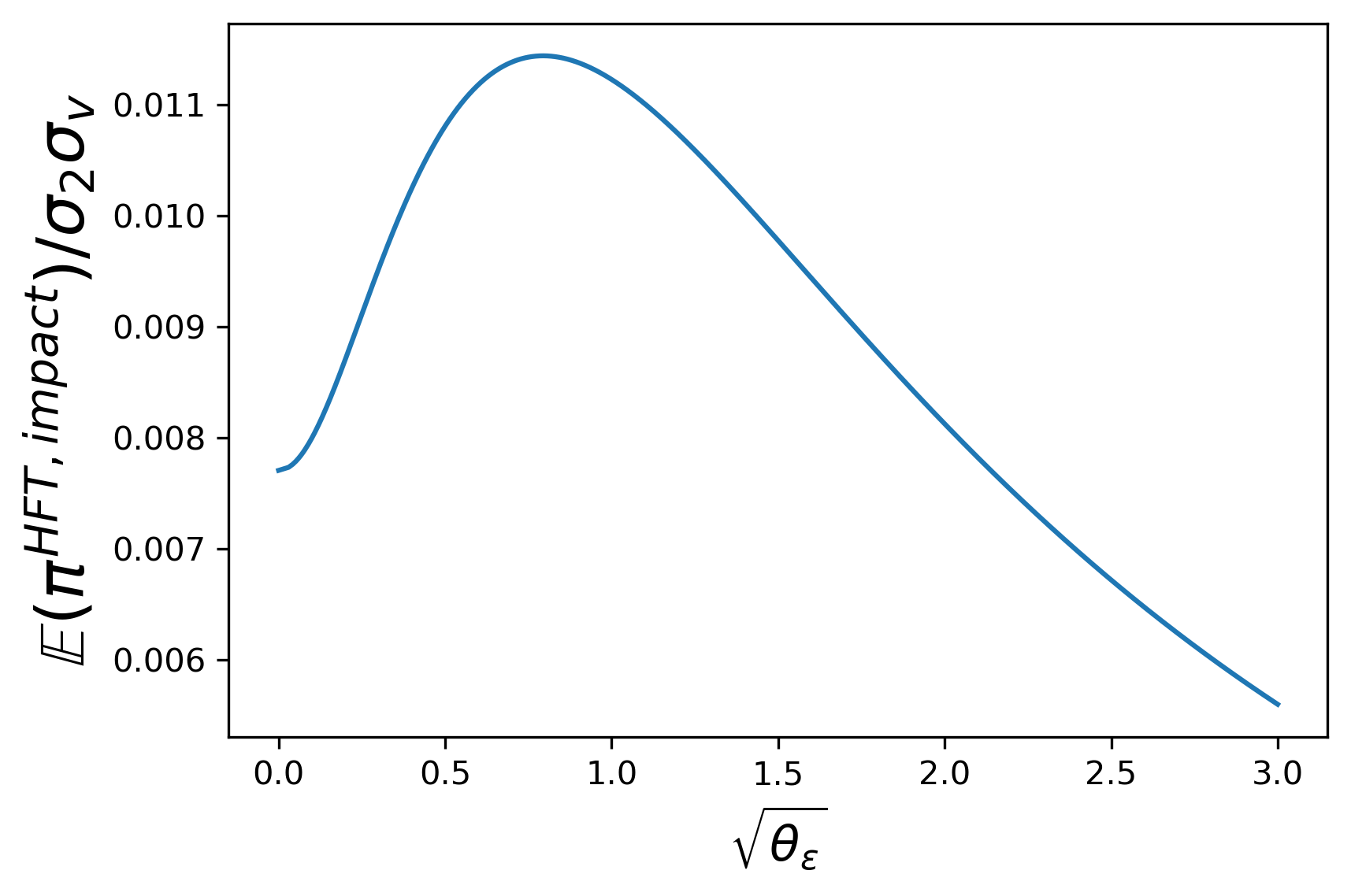
(b) HFT’s impact profit.

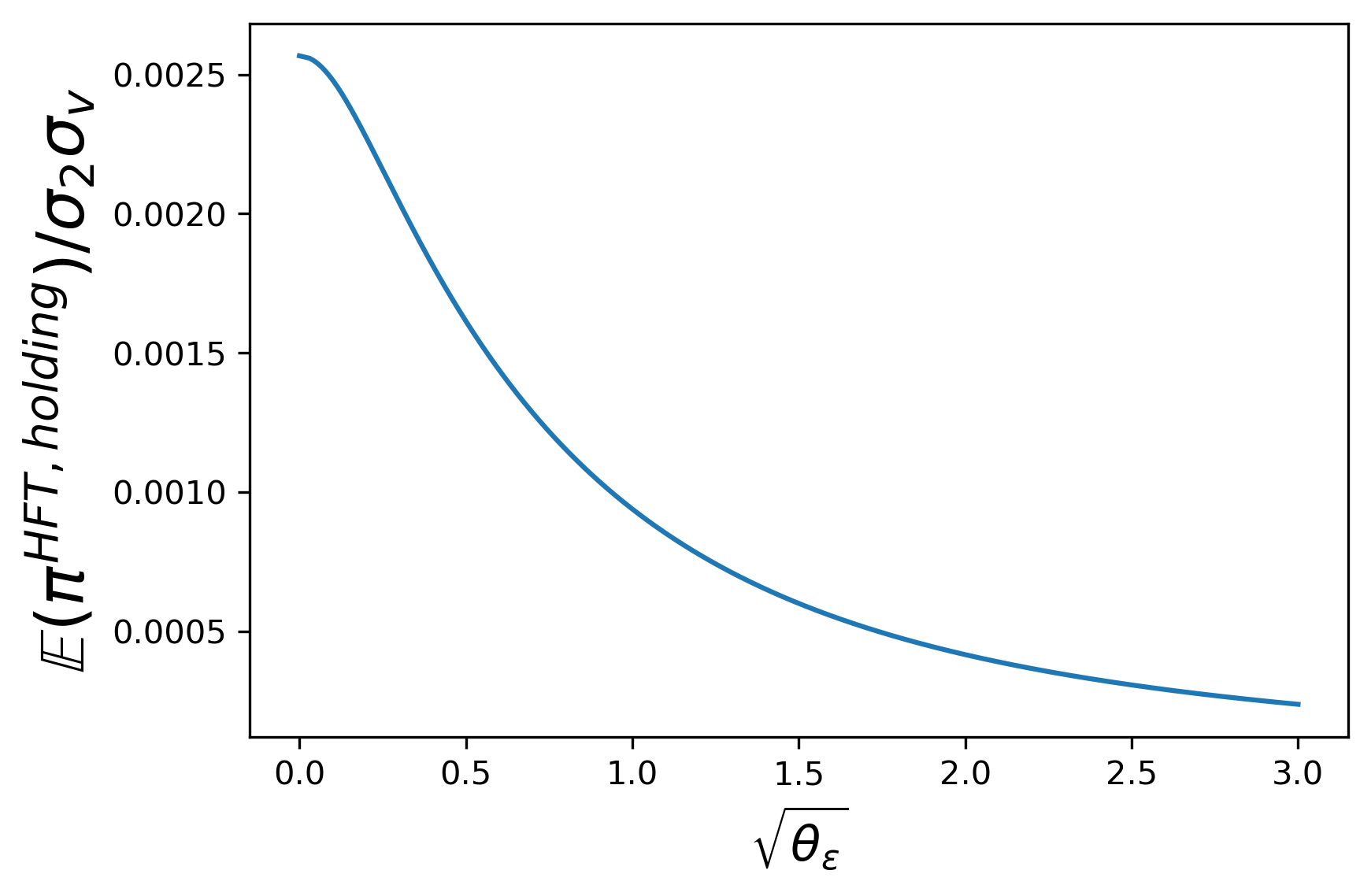
(c) HFT’s holding profit.

Figure 13: $\theta_{1}=0.01,\Gamma=100.$

The reason why we do not see front-runner’s total profit increases with $\theta_{\varepsilon}$ when $\Gamma\in[0,20]$ is that, $\Gamma$ is not yet large enough to allow the increase of impact profit to exceed the decrease of holding profit.

Loss of noise traders. As shown in Figure 14, expectedly, the aggregate loss of noise traders in period 1 grows with $\theta_{1},$ since a larger $\theta_{1}$ indicates that more uninformed investors are suffering from trading with informed investors.

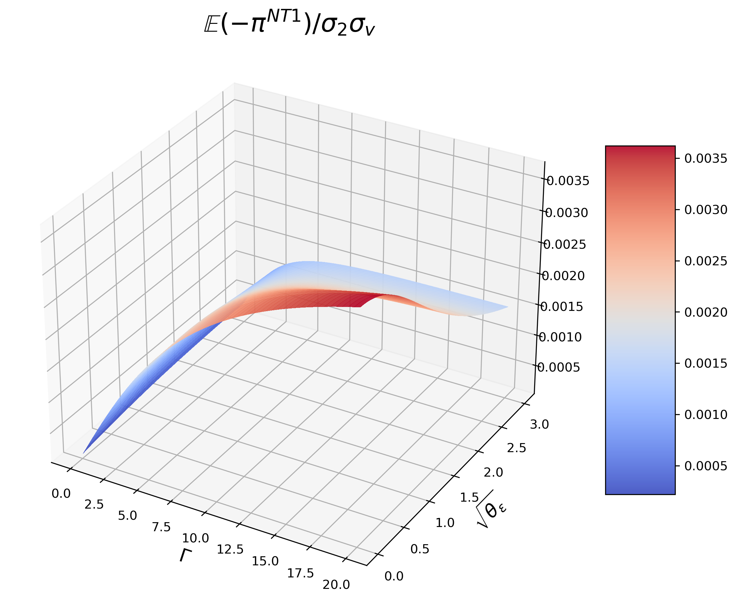
(a) $\theta_{1}=10^{-4}.$

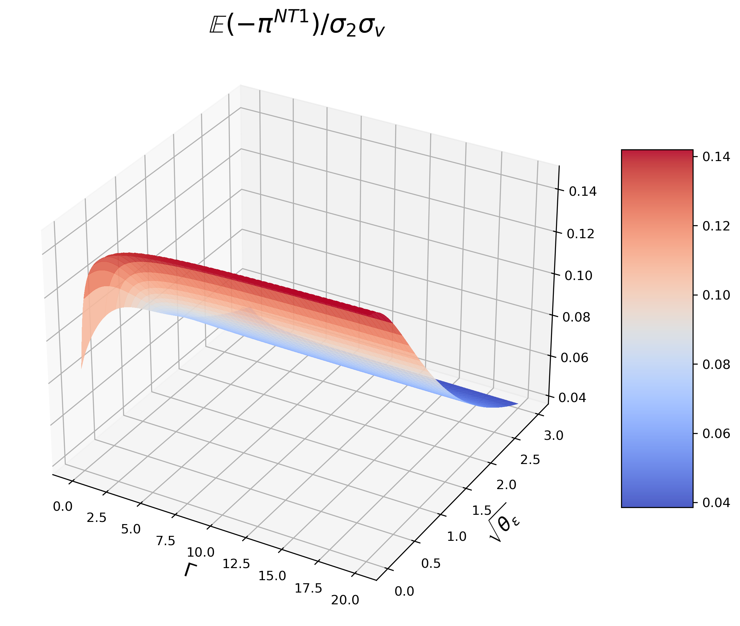
(b) $\theta_{1}=0.1.$

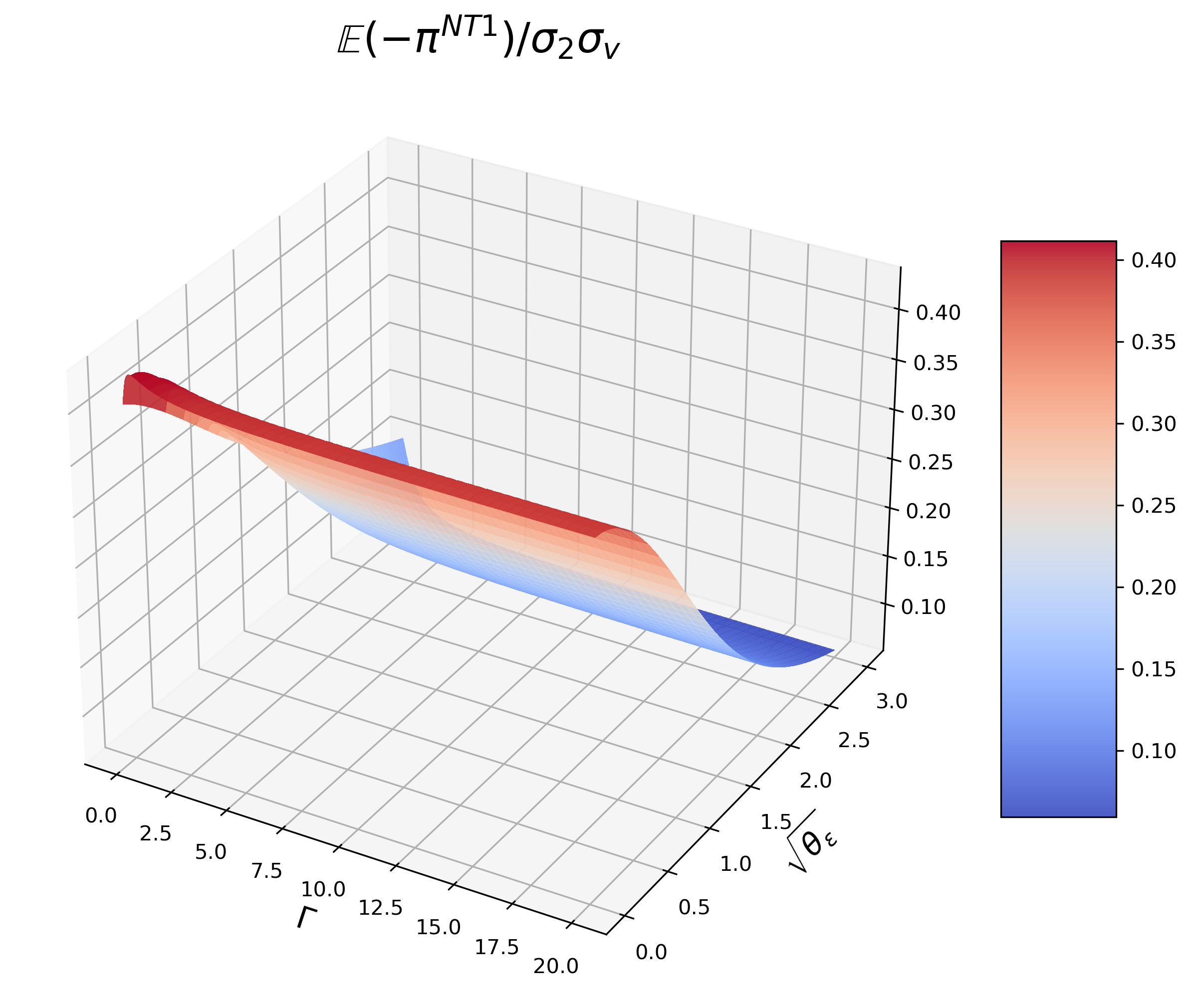
(c) $\theta_{1}=1.$

Figure 14: Loss of noise traders in period 1.

Figure 15 states that HFT benefits normal-speed noise traders since the loss of noise traders in period 2 is always less than that without HFT. In Kyle’s model, where there are only IT, dealers, and noise traders, the informativeness of order flow $y=i+u_{2}$ is $\frac{\sigma_{v}}{2\sigma_{2}}$. While, with HFT, information about $v$ has been exposed through the time-1 trading $y_{1}$. Thus, the price is less sensitive to the surprise component in $y_{2}$ (i.e., $y_{2}-\mathbb{E}(y_{2}|y_{1})$), which makes the informativeness $\lambda_{22}<\frac{\sigma_{v}}{2\sigma_{2}},$ implying less loss of noise traders in period 2.

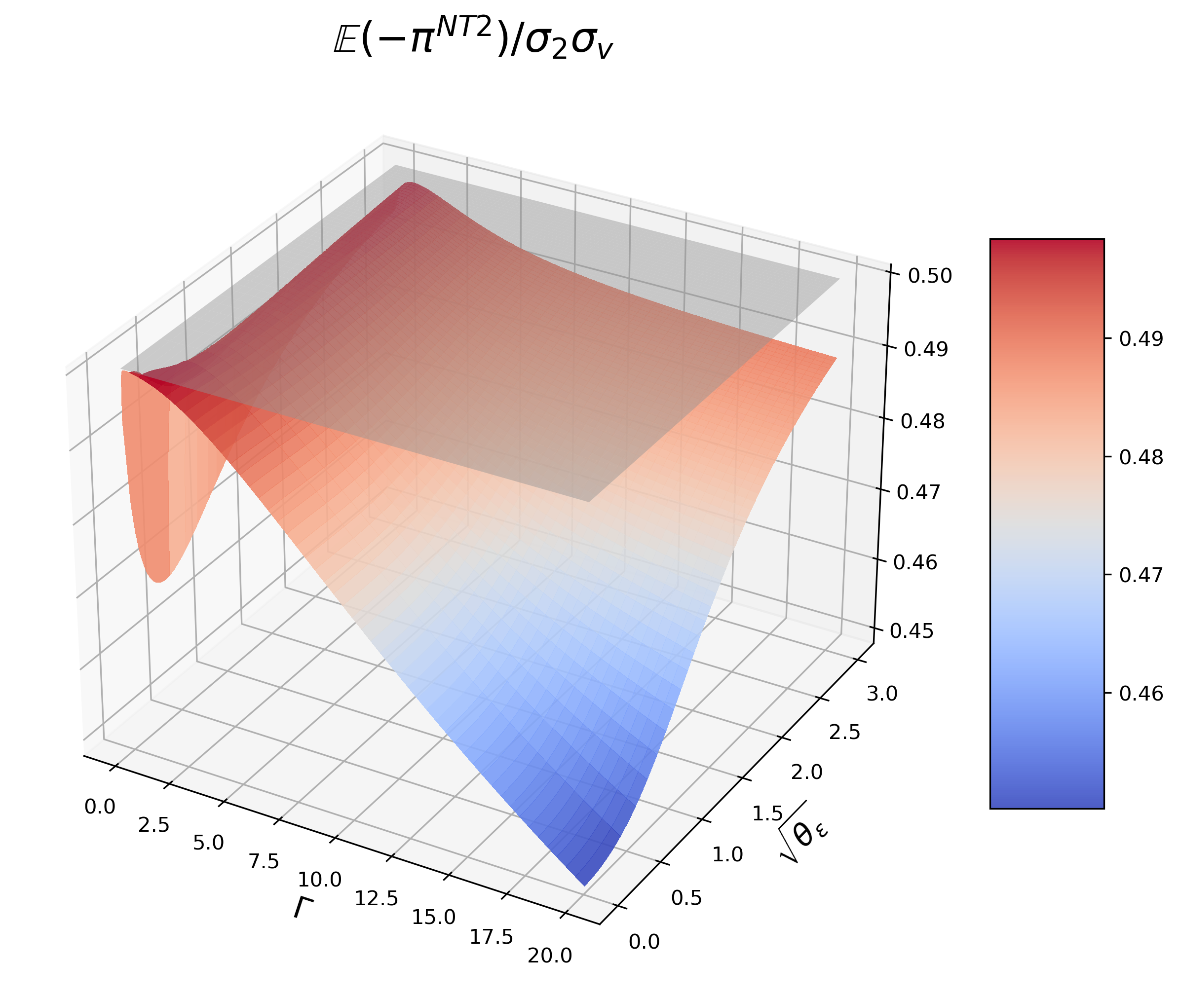
(a) $\theta_{1}=10^{-4}.$

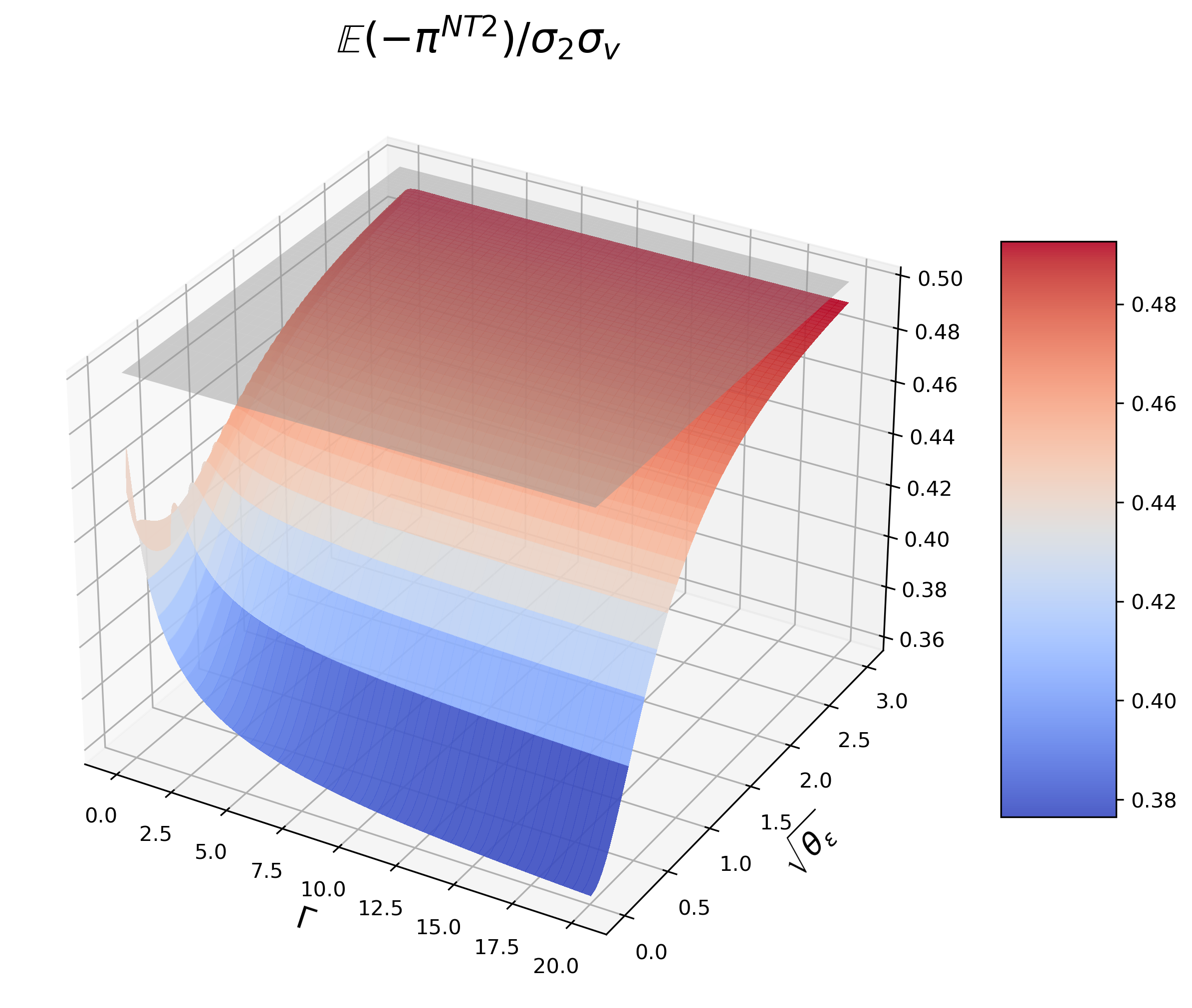
(b) $\theta_{1}=0.1.$

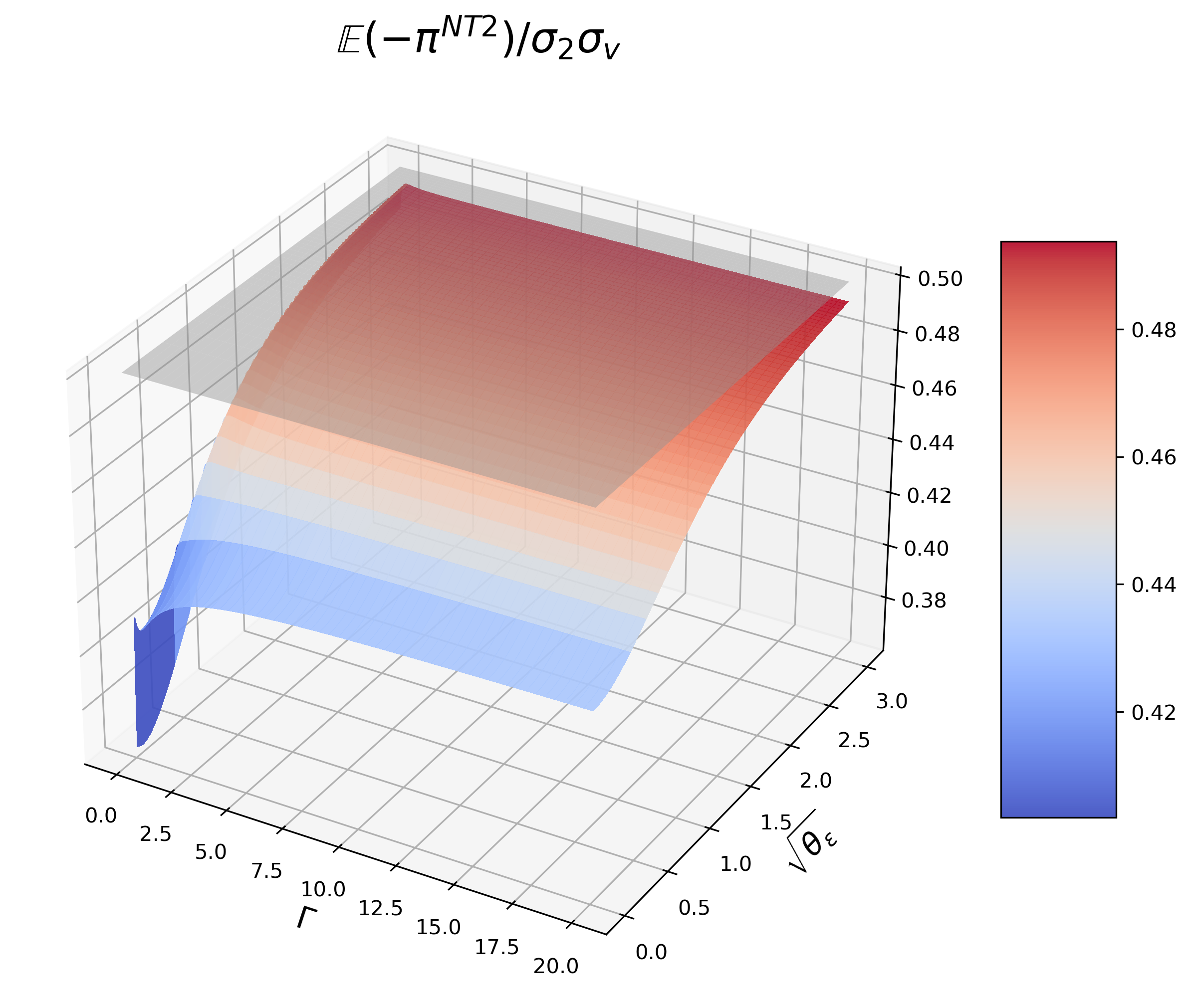
(c) $\theta_{1}=1.$

Figure 15: Loss of noise traders in period 2. The grey plane refers $\mathbb{E}(-\pi^{\text{NT2}})=\frac{\sigma_{2}\sigma_{v}}{2},$
which is the loss of noise traders without HFT.

Price discovery. The price information is unfolded earlier through HFT’s trading. In general, the time-1 pricing error is reduced as $\Gamma$ increases and $\theta_{\varepsilon}$ decreases. In most cases, IT trades more aggressively with a larger $\Gamma$ and hence leaks more information to HFT. On the other hand, a smaller $\theta_{\varepsilon}$ lets HFT predict more precisely. All of the above make $x_{1}$ contain more information about $v$. However, the time-2 pricing error is always $\frac{\sigma_{v}^{2}}{2},$ as proved by Theorem 1, which is the result of IT’s optimization. IT will only release information to this extent, regardless of whether IT is facing a small IT or a front-runner.

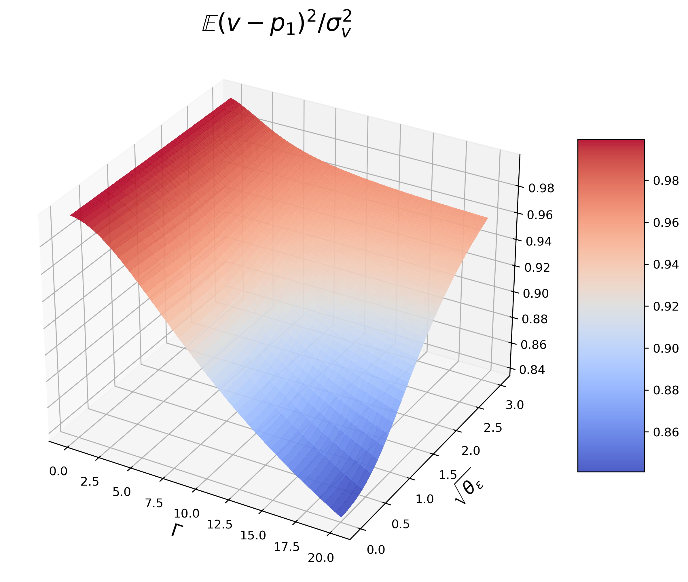
(a) $\theta_{1}=10^{-4}.$

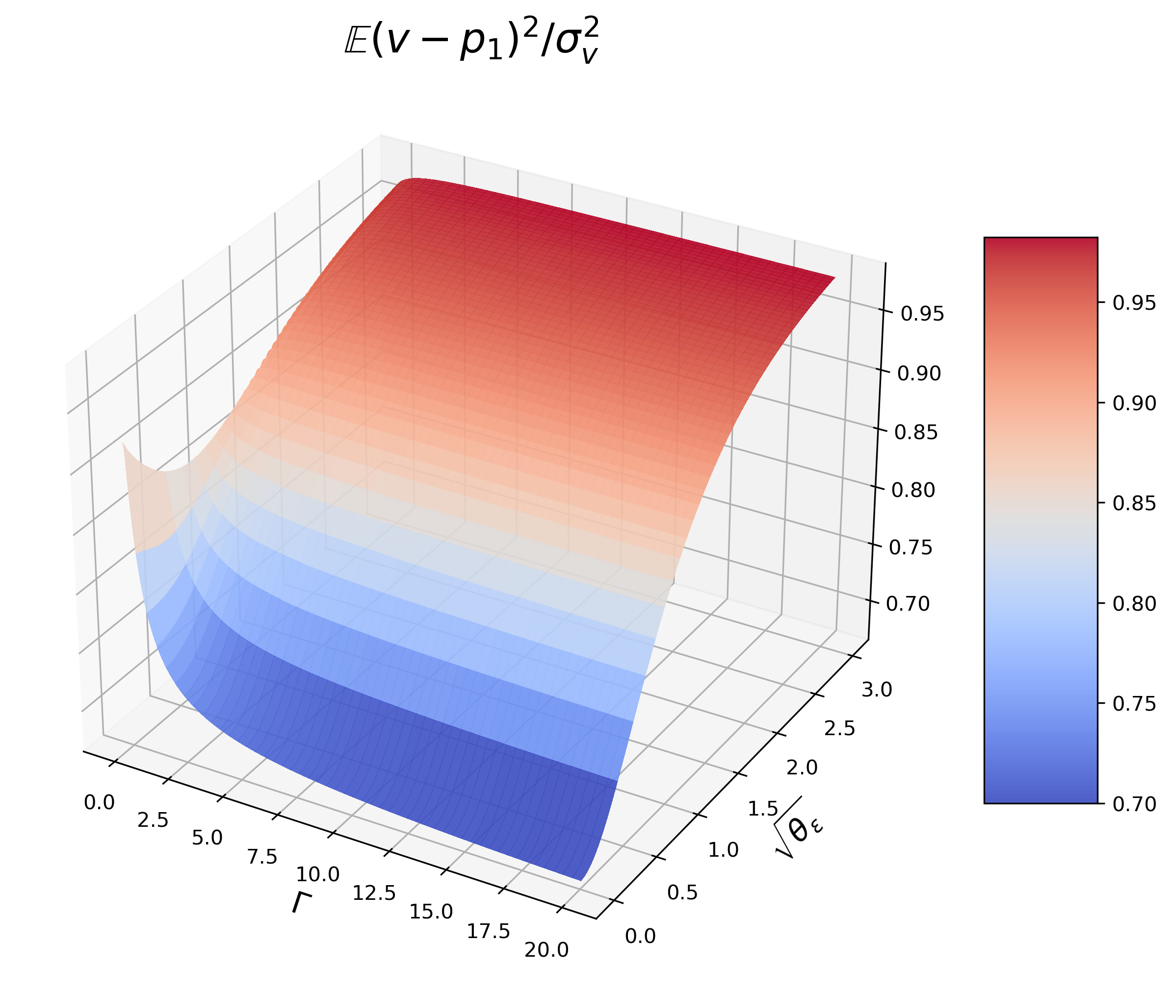
(b) $\theta_{1}=0.1.$

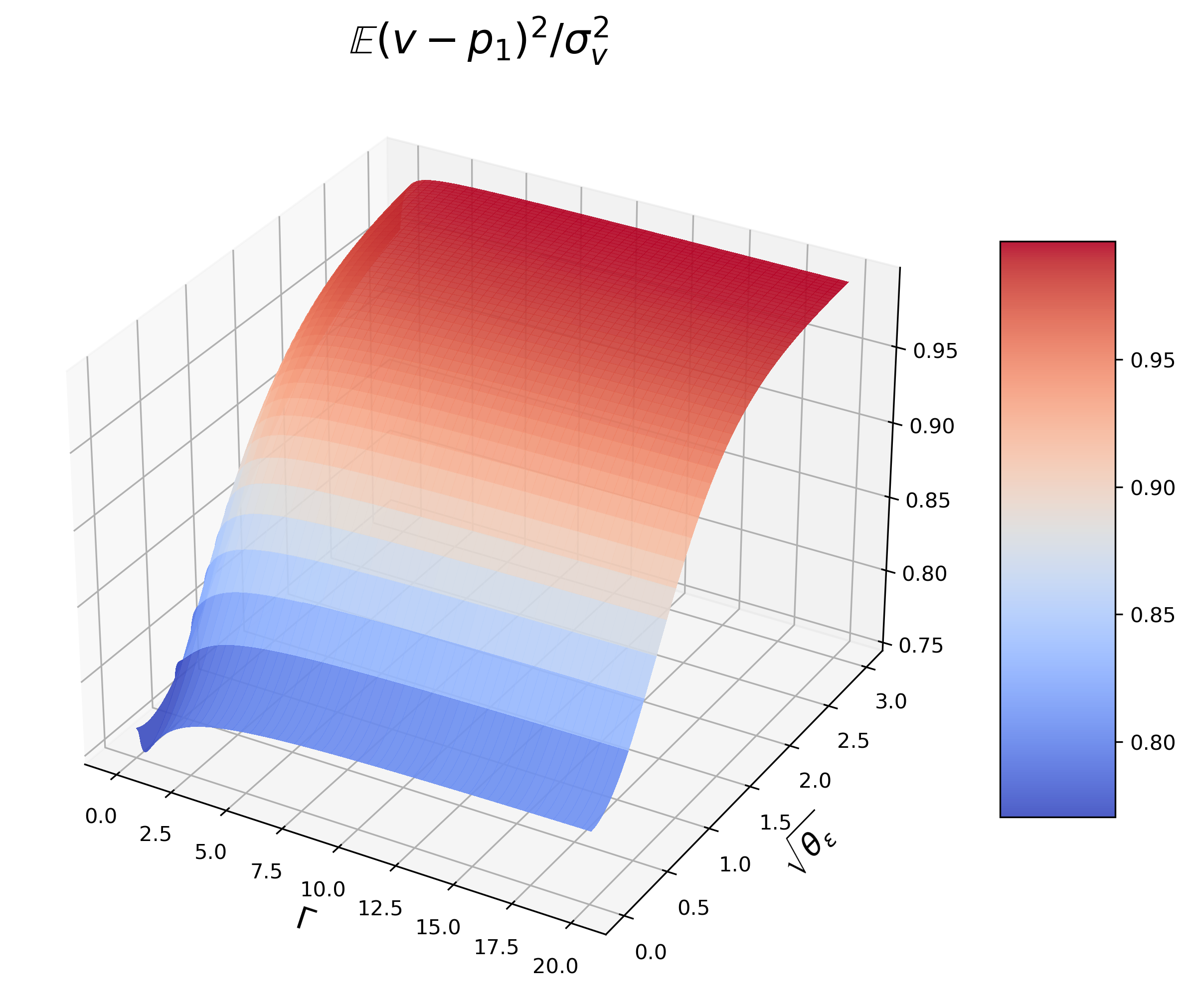
(c) $\theta_{1}=1.$

Figure 16: Time-1 pricing error.

4.1.2 Conclusions

HFT’s strategies. For any $\theta_{1}\in(0,1]$, there exists a $\underline{\Gamma}=\underline{\Gamma}(\theta_{1})$ and a $\overline{\Gamma}=\overline{\Gamma}(\theta_{1}),$ with $\frac{\partial\underline{\Gamma}(\theta_{1})}{\theta_{1}}<0,\frac{\partial\overline{\Gamma}(\theta_{1})}{\theta_{1}}<0,$ to distinguish HFT’s role, as shown in Figure 17: (1) when $\Gamma\in[0,\underline{\Gamma}],$ HFT is a small IT; (2) when $\Gamma\in[\overline{\Gamma},+\infty],$ HFT is a front-runner; (3) when $\Gamma\in(\underline{\Gamma},\overline{\Gamma}),$ there exists a $\overline{\theta}_{\varepsilon}=\overline{\theta}_{\varepsilon}(\theta_{1},\Gamma),$ with $\frac{\partial\overline{\theta}_{\varepsilon}(\theta_{1},\Gamma)}{\theta_{1}}<0,\frac{\partial\overline{\theta}_{\varepsilon}(\theta_{1},\Gamma)}{\Gamma}<0,$ if $\theta_{\varepsilon}>\overline{\theta}_{\varepsilon},$ HFT will act a front-runner. Otherwise, she acts as a small IT.

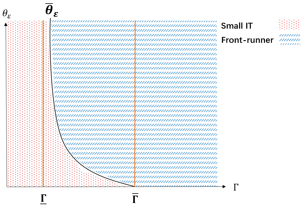
Figure 17: HFT’s strategies.

HFT’s influences on IT. IT could be benefited by front-runner, but is always harmed by small IT, as shown in Figure 18. Given $\theta_{1}\in(0,1]$ and $\Gamma>\underline{\Gamma}(\theta_{1})$, there exists a $\tilde{\theta}_{\varepsilon}=\tilde{\theta}_{\varepsilon}(\theta_{1},\Gamma)\geq\overline{\theta}_{\varepsilon}(\theta_{1},\Gamma),$ with $\frac{\partial\tilde{\theta}_{\varepsilon}(\theta_{1},\Gamma)}{\partial\theta_{1}}<0,\frac{\partial\tilde{\theta}_{\varepsilon}(\theta_{1},\Gamma)}{\partial\Gamma}<0,$ if $\theta_{\varepsilon}>\tilde{\theta}_{\varepsilon}$, IT will be benefited by front-runner.

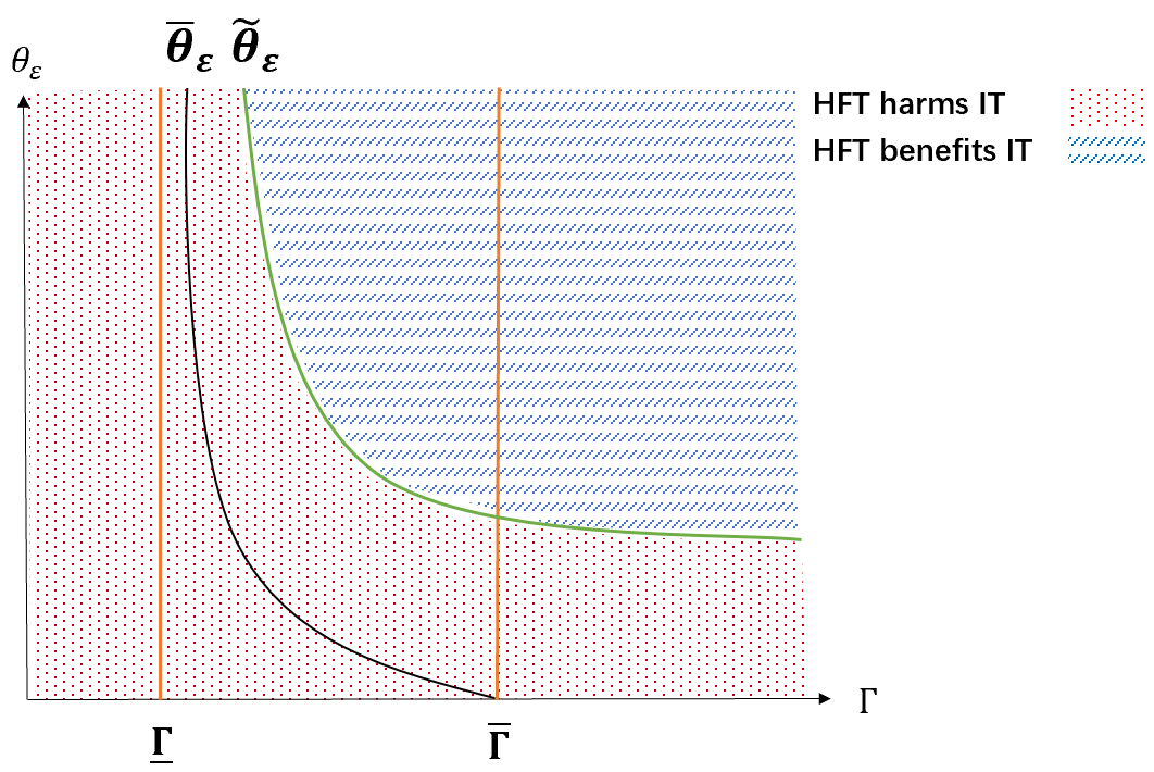
Figure 18: HFT’s influences on IT.

$\theta_{\varepsilon}$’s influences on IT’s profit. As shown in Figure 19, when IT is harmed by HFT, increasing $\theta_{\varepsilon}$ always makes IT less harmed. When IT is benefited by HFT, there exists a $\hat{\theta}_{\varepsilon}=\hat{\theta}_{\varepsilon}(\theta_{1},\Gamma)\geq\tilde{\theta}_{\varepsilon}(\theta_{1},\Gamma),$ with $\frac{\partial\hat{\theta}_{\varepsilon}(\theta_{1},\Gamma)}{\partial\theta_{1}}<0,\frac{\partial\hat{\theta}_{\varepsilon}(\theta_{1},\Gamma)}{\partial\Gamma}<0,$ if $\theta_{\varepsilon}>\hat{\theta}_{\varepsilon},$ IT’s profit will decrease with it.

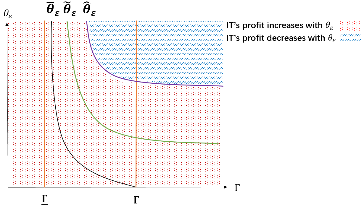
Figure 19: $\theta_{\varepsilon}$’s influences on IT’s profit.

4.2 Equilibrium in the case $\theta_{1}=0$

Now we discuss the equilibrium when noise traders are all normal-speed. In this case,

$$y_{1}=x_{1},\ y_{2}=i+x_{2}+u_{2}.$$

Dealers’ quotes. Given IT and HFT’s strategies,

$$p_{1}=\mathbb{E}(v|y_{1})=p_{0}+\lambda_{1}y_{1},$$

$$p_{2}=\mathbb{E}(v|y_{1},y_{2})=p_{0}+\lambda_{21}y_{1}+\lambda_{22}y_{2}.$$

When $x_{1}\neq 0,$ i.e., $\beta_{1}\neq 0$,

$$\lambda_{1}=\frac{\alpha}{\beta_{1}(\alpha^{2}\sigma_{v}^{2}+\sigma_{\varepsilon}^{2})},\lambda_{21}=\frac{\alpha\sigma_{v}^{2}[\sigma_{2}^{2}-\sigma_{\varepsilon}^{2}(\beta_{21}+\beta_{1}\beta_{23})]}{\beta_{1}[\alpha^{2}\sigma_{v}^{2}(\sigma_{2}^{2}+\sigma_{\varepsilon}^{2})+\sigma_{2}^{2}\sigma_{\varepsilon}^{2}]},\lambda_{22}=\frac{\alpha\sigma_{v}^{2}\sigma_{\varepsilon}^{2}}{\alpha^{2}\sigma_{v}^{2}(\sigma_{2}^{2}+\sigma_{\varepsilon}^{2})+\sigma_{2}^{2}\sigma_{\varepsilon}^{2}}.$$ (15)

When $x_{1}=0,$ i.e., $\beta_{1}=0$,

$$\lambda_{1}=\lambda_{21}=\infty,\lambda_{22}=\frac{\alpha\sigma_{v}^{2}(1+\beta_{21})}{\alpha^{2}\sigma_{v}^{2}(1+\beta_{21})^{2}+\sigma_{\varepsilon}^{2}\beta_{21}^{2}+\sigma_{2}^{2}}.$$ (16)

IT and HFT’s strategies. The optimizations of IT and HFT are similar to those with $\theta_{1}>0$.

In this case, the equilibrium systems have no solutions as shown in the proof of Theorem 2 in Appendix.

Theorem 2.

Neither of the mixed-strategy or pure-strategy equilibrium exists for $\theta_{1}=0$.

4.3 Equilibrium when $\theta_{1}\rightarrow 0$

When $\theta_{\varepsilon}>0,$ the equilibrium exists for $\theta_{1}>0$, as mentioned in 4.1.1. When $\theta_{\varepsilon}=0$, given sufficiently small $\theta_{1}$, $\tilde{\Gamma}(\theta_{1})\rightarrow 0,$ which enables the existence of equilibrium. And thus we can investigate the limit results whenever $\theta_{\varepsilon}>0$ or $\Gamma>0.$

Theorem 3.

When $\theta_{\varepsilon}>0$ or $\Gamma\in(0,\infty),$ in equilibrium, as $\theta_{1}\rightarrow 0$, HFT’s strategies

$$x_{1}\rightarrow 0,\ \text{a.s.,}$$

$$x_{2}\rightarrow\beta_{21}\hat{i},\ \text{a.s.;}$$

IT’s strategy

$$i\rightarrow\alpha(v-p_{0}),\ \text{a.s.;}$$

the liquidation prices

$$p_{1}\rightarrow p_{0},\ \text{a.s.,}$$

$$p_{2}\rightarrow p_{0}+\lambda_{22}y_{2},\ \text{a.s.,}$$

where $\beta_{21}\geq 0$ solves the equation

$$0=\beta_{21}-\frac{2\beta_{21}+1}{2\sqrt{\frac{1}{\beta_{21}^{2}\theta_{\varepsilon}+1}}(2\beta_{21}^{2}\theta_{\varepsilon}+2\beta_{21}\theta_{\varepsilon}+\theta_{\varepsilon}+1)(\sqrt{\frac{1}{\beta_{21}^{2}\theta_{\varepsilon}+1}}+2\Gamma)},$$ (17)

and

$$\alpha=\frac{\sigma_{2}}{\sigma_{v}}\frac{\sqrt{1+\beta_{21}^{2}\theta_{\varepsilon}}}{1+\beta_{21}},$$

$$\lambda_{22}=\frac{\sigma_{v}}{2\sigma_{2}}\frac{1}{\sqrt{1+\beta_{21}^{2}\theta_{\varepsilon}}}.$$

The expected profit of IT

$$\mathbb{E}(\pi^{\text{IT}})\rightarrow\frac{\sigma_{2}\sigma_{v}}{2}\frac{\sqrt{1+\beta_{21}^{2}\theta_{\varepsilon}}}{1+\beta_{21}}\leq\frac{\sigma_{2}\sigma_{v}}{2};$$

the expected profit and expected inventory penalty of HFT

$$\mathbb{E}(\pi^{\text{HFT}})\rightarrow\frac{\sigma_{2}\sigma_{v}}{2}\frac{\beta_{21}(1-\beta_{21}\theta_{\varepsilon})}{\sqrt{1+\beta_{21}^{2}\theta_{\varepsilon}}(1+\beta_{21})},$$

$$\mathbb{E}(-\gamma x_{2}^{2})\rightarrow-\sigma_{2}\sigma_{v}\Gamma\beta_{21}^{2}[\theta_{\varepsilon}+\frac{1+\beta_{21}^{2}\theta_{\varepsilon}}{(1+\beta_{21})^{2}}];$$

the price discovery variables are

$$\mathbb{E}(v-p_{1})^{2}\rightarrow\sigma_{v}^{2},$$

$$\mathbb{E}(v-p_{2})^{2}\rightarrow\frac{\sigma_{v}^{2}}{2};$$

and the aggregate loss of noise traders converges to

$$\lambda_{22}\sigma_{2}^{2}.$$

When there is little noise trading in period 1 ($\theta_{1}\rightarrow 0$), HFT’s time-1 order will bring huge transaction cost to her, so she prefers to do nothing. For IT, the information leakage causes HFT to trade along her, her profit is lower than that without HFT.

It should be noted that when $\theta_{1}\rightarrow 0,$ the equilibrium converges to that when HFT is normal-speed as all other investors. It becomes a static game between IT and another partially informed trader with the same speed. We conclude that HFT almost gives up her speed advantage when there are few high-frequency noise traders.

5 Conclusion

We build up a theoretical model to investigate high-frequency order anticipation strategies and their influences on large trader IT and market quality. The way HFT implements anticipatory trading can be quite different when the inventory aversion and signal precision change: she may act as a small IT or a front-runner. IT is benefited only when HFT provides her with liquidity, i.e., when HFT acts as a front-runner. Some surprising results appear when the size of high-speed noise trading differs: (1) when it is relatively small, front-runner may harm the large trader more than small IT and HFT may profit more with a less accurate signal if she is sufficiently inventory averse; (2) when it is relatively large and the front-runner is beneficial to IT, adding any noise in HFT’s signal can decrease IT’s profit. With the presence of HFT, the loss of normal-speed noise traders is reduced and price discovery is accelerated. However, in any case, the final level of price discovery remains unchanged. If almost all the noise traders are as slow as IT, HFT gives up her speed advantage and becomes normal-speed, too.

Appendix

Proof of Theorem 1. Substitute (3), (8), (9), (10) into (14), we have

$$\Lambda_{21}=\frac{A^{3}\Lambda_{22}[2(\beta_{1}-1)\Gamma-\Lambda_{22}]+A^{2}\Gamma+2A\theta_{\varepsilon}\Lambda_{22}[(\beta_{1}-1)\Gamma-\Lambda_{22}]+\theta_{\varepsilon}(\Gamma+\Lambda_{22})}{A\beta_{1}(A^{2}+\theta_{\varepsilon})(2\Gamma+\Lambda_{22})}.$$ (18)

Then substitute (3), (8), (9), (10), (18) into (4), (5), (12) and three SOCs, we get the simplified system of equilibrium:

$$0= \beta_{1}-(A^{4}(-\Lambda_{22})(\Lambda_{22}(2\Gamma+\Lambda_{22})-4\beta_{1}\Gamma(\Gamma+\Lambda_{22}))+A^{3}\Lambda_{22}((2\beta_{1}+3)\Gamma+2\beta_{1}\Lambda_{22}+\Lambda_{22})$$ (19)

$$+ A^{2}(4\beta_{1}\theta_{\varepsilon}\Gamma^{2}\Lambda_{22}+\Gamma(2(2\beta_{1}-1)\theta_{\varepsilon}\Lambda_{22}^{2}-1)-2\theta_{\varepsilon}\Lambda_{22}^{3})+A(2\beta_{1}+3)\theta_{\varepsilon}\Lambda_{22}(\Gamma+\Lambda_{22})-\theta_{\varepsilon}(\Gamma+\Lambda_{22}))/$$

$$(\beta_{1}(A^{2}+\theta_{\varepsilon})^{2}(\Gamma+\Lambda_{22})(2\Gamma+\Lambda_{22})(\frac{4A\beta_{1}}{A^{2}\beta_{1}^{2}+\beta_{1}^{2}\theta_{\varepsilon}+\theta_{1}}$$

$$- \frac{(A^{3}(4\beta_{1}\Gamma(\Gamma+\Lambda_{22})-\Lambda_{22}(2\Gamma+\Lambda_{22}))+A^{2}\Gamma+2A\theta_{\varepsilon}(\Gamma+\Lambda_{22})(2\beta_{1}\Gamma-\Lambda_{22})+\theta_{\varepsilon}(\Gamma+\Lambda_{22}))^{2}}{A^{2}\beta_{1}^{2}(A^{2}+\theta_{\varepsilon})^{2}(\Gamma+\Lambda_{22})(2\Gamma+\Lambda_{22})^{2}}+4\Gamma)),$$

$$0= (2(\beta_{1}-1)\Gamma-\Lambda_{22})\Lambda_{22}(4((\theta_{\varepsilon}+\theta_{1}+1)\Gamma^{2}+2(\theta_{\varepsilon}+1)\Lambda_{22}\Gamma+(\theta_{\varepsilon}+1)\Lambda_{22}^{2})\beta_{1}^{2}-4\Gamma(2\Gamma+\Lambda_{22})\theta_{1}\beta_{1}$$

$$+ (2\Gamma+\Lambda_{22})^{2}\theta_{1})A^{7}-(8\theta_{\varepsilon}\Gamma(\Gamma+\Lambda_{22})^{2}\beta_{1}^{3}-4((\theta_{\varepsilon}+\theta_{1}-1)\Gamma^{3}+\Lambda_{22}(2\theta_{\varepsilon}-\theta_{1}-3)\Gamma^{2}$$

$$+ (\theta_{\varepsilon}-3)\Lambda_{22}^{2}\Gamma-\Lambda_{22}^{3})\beta_{1}^{2}+4\Gamma(2\Gamma^{2}-\Lambda_{22}\Gamma-\Lambda_{22}^{2})\theta_{1}\beta_{1}-(\Gamma-\Lambda_{22})(2\Gamma+\Lambda_{22})^{2}\theta_{1})A^{6}$$

$$+ (8\theta_{\varepsilon}\Gamma\Lambda_{22}((2\theta_{\varepsilon}+3\theta_{1}+3)\Gamma^{2}+2(2\theta_{\varepsilon}+3)\Lambda_{22}\Gamma+(2\theta_{\varepsilon}+3)\Lambda_{22}^{2})\beta_{1}^{3}-2\theta_{\varepsilon}(4\Lambda_{22}(2\theta_{\varepsilon}+7\theta_{1}+3)\Gamma^{3}$$

$$+ (2\Lambda_{22}^{2}(11\theta_{\varepsilon}+8\theta_{1}+16)-1)\Gamma^{2}+(4(5\theta_{\varepsilon}+7)\Lambda_{22}^{3}-2\Lambda_{22})\Gamma+\Lambda_{22}^{2}((6\theta_{\varepsilon}+8)\Lambda_{22}^{2}-1))\beta_{1}^{2}$$

$$+ 2\Gamma((11\theta_{\varepsilon}+4)\Lambda_{22}^{3}+4\Gamma^{2}(6\theta_{\varepsilon}\Lambda_{22}+\Lambda_{22})+\Gamma(8(4\theta_{\varepsilon}+1)\Lambda_{22}^{2}-1))\theta_{1}\beta_{1}-(2\Gamma+\Lambda_{22})(2(3\theta_{\varepsilon}+2)\Lambda_{22}^{3}$$

$$+ 4\Gamma^{2}(2\theta_{\varepsilon}\Lambda_{22}+\Lambda_{22})+\Gamma(2(7\theta_{\varepsilon}+4)\Lambda_{22}^{2}-1))\theta_{1})A^{5}+(-16\theta_{\varepsilon}^{2}\Gamma(\Gamma+\Lambda_{22})^{2}\beta_{1}^{3}$$

$$+ 4\theta_{\varepsilon}((2\theta_{\varepsilon}+3\theta_{1}-1)\Gamma^{3}+\Lambda_{22}(6\theta_{\varepsilon}-\theta_{1}-3)\Gamma^{2}+3(2\theta_{\varepsilon}-1)\Lambda_{22}^{2}\Gamma+(2\theta_{\varepsilon}-1)\Lambda_{22}^{3})\beta_{1}^{2}$$

$$- 8\theta_{\varepsilon}\Gamma^{2}(2\Gamma+\Lambda_{22})\theta_{1}\beta_{1}+(\Gamma+\Lambda_{22})((8\theta_{\varepsilon}+4)\Gamma^{2}+4(2\theta_{\varepsilon}\Lambda_{22}+\Lambda_{22})\Gamma+\theta_{\varepsilon}\Lambda_{22}^{2})\theta_{1})A^{4}$$

$$+ \theta_{\varepsilon}(8\theta_{\varepsilon}\Gamma\Lambda_{22}((\theta_{\varepsilon}+3\theta_{1}+3)\Gamma^{2}+2(\theta_{\varepsilon}+3)\Lambda_{22}\Gamma+(\theta_{\varepsilon}+3)\Lambda_{22}^{2})\beta_{1}^{3}-4\theta_{\varepsilon}\Lambda_{22}(2(\theta_{\varepsilon}+5\theta_{1}+3)\Gamma^{3}$$

$$+ \Lambda_{22}(6\theta_{\varepsilon}+7\theta_{1}+17)\Gamma^{2}+2(3\theta_{\varepsilon}+8)\Lambda_{22}^{2}\Gamma+(2\theta_{\varepsilon}+5)\Lambda_{22}^{3})\beta_{1}^{2}+2\Gamma(8(\theta_{\varepsilon}+1)\Lambda_{22}^{3}$$

$$+ 4(5\theta_{\varepsilon}+4)\Gamma\Lambda_{22}^{2}+4(3\theta_{\varepsilon}+2)\Gamma^{2}\Lambda_{22}-\Lambda_{22}-2\Gamma)\theta_{1}\beta_{1}-\Lambda_{22}(\Gamma+\Lambda_{22})(8(\theta_{\varepsilon}+2)\Gamma^{2}$$

$$+ 4(4\theta_{\varepsilon}+7)\Lambda_{22}\Gamma+4(2\theta_{\varepsilon}+3)\Lambda_{22}^{2}-1)\theta_{1})A^{3}+4\theta_{\varepsilon}(-2\theta_{\varepsilon}^{2}\Gamma(\Gamma+\Lambda_{22})^{2}\beta_{1}^{3}+\theta_{\varepsilon}((\theta_{\varepsilon}+3\theta_{1}+1)\Gamma^{3}$$

$$+ \Lambda_{22}(4\theta_{\varepsilon}+\theta_{1}+3)\Gamma^{2}+(5\theta_{\varepsilon}+3)\Lambda_{22}^{2}\Gamma+(2\theta_{\varepsilon}+1)\Lambda_{22}^{3})\beta_{1}^{2}-\theta_{\varepsilon}\Gamma(2\Gamma^{2}+3\Lambda_{22}\Gamma+\Lambda_{22}^{2})\theta_{1}\beta_{1}$$

$$+ (\Gamma+\Lambda_{22})^{2}((\theta_{\varepsilon}+2)\Gamma+2\theta_{\varepsilon}\Lambda_{22}+\Lambda_{22})\theta_{1})A^{2}+2\theta_{\varepsilon}^{2}(4\theta_{\varepsilon}\Gamma\Lambda_{22}((\theta_{1}+1)\Gamma^{2}+2\Lambda_{22}\Gamma+\Lambda_{22}^{2})\beta_{1}^{3}$$

$$- \theta_{\varepsilon}(\Gamma+\Lambda_{22})(4\Lambda_{22}^{3}+8\Gamma\Lambda_{22}^{2}+4\Gamma^{2}(\theta_{1}+1)\Lambda_{22}+\Lambda_{22}+\Gamma)\beta_{1}^{2}$$

$$+ \Gamma(4\Lambda_{22}^{3}+8\Gamma\Lambda_{22}^{2}+4\Gamma^{2}\Lambda_{22}-\Lambda_{22}-\Gamma)\theta_{1}\beta_{1}-(\Gamma+\Lambda_{22})^{2}(4\Lambda_{22}^{2}+4\Gamma\Lambda_{22}+1)\theta_{1})A$$

$$+ 4\theta_{\varepsilon}^{2}(\Gamma+\Lambda_{22})(\theta_{\varepsilon}((\theta_{1}+1)\Gamma^{2}+2\Lambda_{22}\Gamma+\Lambda_{22}^{2})\beta_{1}^{2}+(\Gamma+\Lambda_{22})^{2}\theta_{1}),$$

$$0= A^{4}\Lambda_{22}(4\beta_{1}^{2}(\Gamma^{2}(\theta_{\varepsilon}+\theta_{1}+1)+2(\theta_{\varepsilon}+1)\Gamma\Lambda_{22}+(\theta_{\varepsilon}+1)\Lambda_{22}^{2})-4\beta_{1}\Gamma\theta_{1}(2\Gamma+\Lambda_{22})+\theta_{1}(2\Gamma+\Lambda_{22})^{2})$$

$$- 2A^{3}(2\beta_{1}^{2}\theta_{\varepsilon}(\Gamma+\Lambda_{22})^{2}-2\beta_{1}\Gamma^{2}\theta_{1}+\Gamma\theta_{1}(2\Gamma+\Lambda_{22}))+A^{2}(4\beta_{1}^{2}\theta_{\varepsilon}\Lambda_{22}(\Gamma^{2}(\theta_{\varepsilon}+2\theta_{1}+2)$$

$$+ 2(\theta_{\varepsilon}+2)\Gamma\Lambda_{22}+(\theta_{\varepsilon}+2)\Lambda_{22}^{2})-4\beta_{1}\theta_{\varepsilon}\Gamma\Lambda_{22}\theta_{1}(2\Gamma+\Lambda_{22})+\theta_{1}(4(\theta_{\varepsilon}+1)\Gamma^{2}\Lambda_{22}$$

$$+ 8(\theta_{\varepsilon}+1)\Gamma\Lambda_{22}^{2}+4(\theta_{\varepsilon}+1)\Lambda_{22}^{3}-2\Gamma-\Lambda_{22}))-4A\theta_{\varepsilon}(\beta_{1}^{2}\theta_{\varepsilon}(\Gamma+\Lambda_{22})^{2}-\beta_{1}\Gamma^{2}\theta_{1}+\theta_{1}(\Gamma+\Lambda_{22})^{2})$$

$$+ 4\theta_{\varepsilon}\Lambda_{22}(\beta_{1}^{2}\theta_{\varepsilon}(\Gamma^{2}(\theta_{1}+1)+2\Gamma\Lambda_{22}+\Lambda_{22}^{2})+\theta_{1}(\Gamma+\Lambda_{22})^{2}),$$

$$0< \Lambda_{22}+\Gamma,$$

$$0< A,$$

$$0< 4\Gamma+\frac{4A\beta_{1}}{A^{2}\beta_{1}^{2}+\beta_{1}^{2}\theta_{\varepsilon}+\theta_{1}}$$

$$- \frac{(A^{3}(4\beta_{1}\Gamma(\Gamma+\Lambda_{22})-\Lambda_{22}(2\Gamma+\Lambda_{22}))+A^{2}\Gamma+2A\theta_{\varepsilon}(\Gamma+\Lambda_{22})(2\beta_{1}\Gamma-\Lambda_{22})+\theta_{\varepsilon}(\Gamma+\Lambda_{22}))^{2}}{A^{2}\beta_{1}^{2}(A^{2}+\theta_{\varepsilon})^{2}(\Gamma+\Lambda_{22})(2\Gamma+\Lambda_{22})^{2}}.$$

For investors’ profits and market variables, we only prove the time-2 pricing error is always $\frac{\sigma_{v}^{2}}{2}.$ Substitute (4), (5) into (14), we have

$$A=\sqrt{\frac{\theta_{1}\theta_{\varepsilon}(\beta_{21}+\beta_{1}(\beta_{23}-\beta_{22}))^{2}+\beta_{1}^{2}\theta_{\varepsilon}+\theta_{1}}{\theta_{1}(1+\beta_{21}+\beta_{1}(\beta_{23}-\beta_{22}))^{2}+(1+\theta_{\varepsilon})\beta_{1}^{2}}}.$$ (20)

Calculate $\mathbb{E}(v-p_{2})^{2}$ and substitute (4), (5), (20) into it, we prove it.

Proof of Corollary 1. Substitute (8),(9),(10),(12) into (14),

$$A(-\Lambda_{21}^{2}+2\Lambda_{21}\Lambda_{22}+4A\Lambda_{1}\Lambda_{21})=0.$$

Since $A>0,$ we have

$$A=\frac{\Lambda_{21}(\Lambda_{21}-2\Lambda_{22})}{4\Lambda_{1}\Lambda_{22}^{2}}.$$ (21)

By SOC (7) and (11), we have

$$\Lambda_{22}>0,\Lambda_{1}>\Lambda_{22}\beta_{23}^{2}>0,$$ (22)

Combining (21), (22) and $A>0$, if $\Lambda_{21}>0$, we have $\Lambda_{21}>2\Lambda_{22}.$ Substitute (21) into (3), it becomes

$$\Lambda_{1}(\Lambda_{21}^{2}+4\Lambda_{22}^{2}(4\Lambda_{1}^{2}\theta_{1}-1))=0.$$

Since $\Lambda_{1}>0,$

$$\Lambda_{22}=\frac{\Lambda_{21}}{2\sqrt{1-4\Lambda_{1}^{2}\theta_{1}}}>\frac{\Lambda_{21}}{2}.$$

We got two contradictory conclusions. If $\Lambda_{21}<0,$ substitute (21) into (4), we have

$$0= 64\Lambda_{1}^{2}\Lambda_{21}\Lambda_{22}^{4}\theta_{1}+\Lambda_{1}(4\Lambda_{21}^{3}\Lambda_{22}\theta_{1}-8\Lambda_{21}^{2}\Lambda_{22}^{2}\theta_{1}+16\Lambda_{21}\Lambda_{22}^{3}-32\Lambda_{22}^{4})+\Lambda_{21}^{5}\theta_{1}$$

$$- 4\Lambda_{21}^{4}\Lambda_{22}\theta_{1}+4\Lambda_{21}^{3}\Lambda_{22}^{2}\theta_{1}+4\Lambda_{21}^{3}\Lambda_{22}^{2}-16\Lambda_{21}^{2}\Lambda_{22}^{3}+16\Lambda_{21}\Lambda_{22}^{4},$$

however the RHS is always strictly negative, so the equilibrium does not exist.

Proof of Theorem 2. For mixed-strategy equilibrium, it does noe exists since IT faces a quadratic optimization. For pure-strategy equilibrium, in any cases, if $A=0,$ the prices will always be $p_{0}$ during the whole trading periods. Given such quotes, IT would find her trading has no price impact, her optimization tells $A=\infty$, which contradicts with $A=0.$ Thus, there is no equilibrium when $A=0.$

When $\theta_{1}=0,\beta_{1}\neq 0$, combining with the discussion above, SOC (13) requires $A>0$. By Equations (15),(14),(8),(9),(10),

$$A=\sqrt{\frac{\theta_{\varepsilon}}{1+\theta_{\varepsilon}}},$$

$$\beta_{21}=\frac{A}{2(\theta_{\varepsilon}(A+\Gamma)+A^{2}(1+\theta_{\varepsilon})\Gamma)},$$

$$\beta_{23}=\frac{A(\beta_{21}\theta_{\varepsilon}-1)-2\beta_{1}\theta_{\varepsilon}\Gamma-2A^{2}\beta_{1}(1+\theta_{\varepsilon})\Gamma}{A\beta_{1}\theta_{\varepsilon}+2\beta_{1}\theta_{\varepsilon}\Gamma+2A^{2}\beta_{1}(1+\theta_{\varepsilon})\Gamma},$$

$$\beta_{22}=\frac{A(-1+(\beta_{21}+\beta_{1}\beta_{23})\theta_{\varepsilon})}{2(A\beta_{1}\theta_{\varepsilon}+\beta_{1}\theta_{\varepsilon}\Gamma+A^{2}\beta_{1}(1+\theta_{\varepsilon})\Gamma)},$$

$$\Lambda_{1}=\frac{A}{\beta_{1}(A^{2}+\theta_{\varepsilon})},$$

$$\Lambda_{21}=\frac{-A(-1+(\beta_{21}+\beta_{1}\beta_{23})\theta_{\varepsilon})}{\beta_{1}(\theta_{\varepsilon}+A^{2}(1+\theta_{\varepsilon}))},$$

$$\Lambda_{22}=\frac{A\theta_{\varepsilon}}{\theta_{\varepsilon}+A^{2}(1+\theta_{\varepsilon})}.$$

Substitute those into Equation (12), when $\theta_{\varepsilon}>0$ and $0<\Gamma<\infty$ we have

$$\beta_{1}=\frac{-16\theta_{\varepsilon}\sqrt{\frac{\theta_{\varepsilon}}{\theta_{\varepsilon}+1}}\Gamma^{3}-20\theta_{\varepsilon}\Gamma^{2}-2\Gamma(8\sqrt{\frac{\theta_{\varepsilon}}{\theta_{\varepsilon}+1}}\Gamma^{2}+3\sqrt{\frac{\theta_{\varepsilon}}{\theta_{\varepsilon}+1}}+4\Gamma)-8\theta_{\varepsilon}\sqrt{\frac{\theta_{\varepsilon}}{\theta_{\varepsilon}+1}}\Gamma-\theta_{\varepsilon}}{2\theta_{\varepsilon}^{2}\Gamma(\sqrt{\frac{\theta_{\varepsilon}}{\theta_{\varepsilon}+1}}+2\Gamma)+8\theta_{\varepsilon}\Gamma^{2}+4\sqrt{\frac{\theta_{\varepsilon}}{\theta_{\varepsilon}+1}}\theta_{\varepsilon}\Gamma},$$

which implies the SOC (11) is

$$\Lambda_{1}+\Gamma-(\Lambda_{22}+\Gamma)\beta_{23}^{2}$$

$$= -(\theta_{\varepsilon}\Gamma(\theta_{\varepsilon}^{3}(1280\sqrt{\frac{\theta_{\varepsilon}}{\theta_{\varepsilon}+1}}\Gamma^{5}+736\sqrt{\frac{\theta_{\varepsilon}}{\theta_{\varepsilon}+1}}\Gamma^{3}+33\sqrt{\frac{\theta_{\varepsilon}}{\theta_{\varepsilon}+1}}\Gamma+512\Gamma^{6}+1344\Gamma^{4}+218\Gamma^{2}+2)$$

$$+2\theta_{\varepsilon}^{2}(1536\sqrt{\frac{\theta_{\varepsilon}}{\theta_{\varepsilon}+1}}\Gamma^{5}+832\sqrt{\frac{\theta_{\varepsilon}}{\theta_{\varepsilon}+1}}\Gamma^{3}+30\sqrt{\frac{\theta_{\varepsilon}}{\theta_{\varepsilon}+1}}\Gamma+512\Gamma^{6}+1248\Gamma^{4}+172\Gamma^{2}+1)$$

$$+64\Gamma^{3}(8\sqrt{\frac{\theta_{\varepsilon}}{\theta_{\varepsilon}+1}}\Gamma^{2}+5\sqrt{\frac{\theta_{\varepsilon}}{\theta_{\varepsilon}+1}}+4\Gamma)+4\theta_{\varepsilon}\Gamma(576\sqrt{\frac{\theta_{\varepsilon}}{\theta_{\varepsilon}+1}}\Gamma^{4}+312\sqrt{\frac{\theta_{\varepsilon}}{\theta_{\varepsilon}+1}}\Gamma^{2}+7\sqrt{\frac{\theta_{\varepsilon}}{\theta_{\varepsilon}+1}}$$

$$+128\Gamma^{5}+352\Gamma^{3}+36\Gamma)))/(2(\theta_{\varepsilon}+1)^{2}(\sqrt{\frac{\theta_{\varepsilon}}{\theta_{\varepsilon}+1}}+4\Gamma)^{2}(2\Gamma(8\sqrt{\frac{\theta_{\varepsilon}}{\theta_{\varepsilon}+1}}\Gamma^{2}+3\sqrt{\frac{\theta_{\varepsilon}}{\theta_{\varepsilon}+1}}+4\Gamma)$$

$$+\theta_{\varepsilon}(16\sqrt{\frac{\theta_{\varepsilon}}{\theta_{\varepsilon}+1}}\Gamma^{3}+8\sqrt{\frac{\theta_{\varepsilon}}{\theta_{\varepsilon}+1}}\Gamma+20\Gamma^{2}+1))^{2})$$

$$<0,$$

the equilibrium does not exist. When $\theta_{\varepsilon}>0$ and $\Gamma=0$ or $\Gamma=\infty$, we have $\beta_{1}=0,$ which contradicts with the assumption $\beta_{1}\neq 0.$ When $\theta_{\varepsilon}=0,$ we have $A=0,$ which is also incorrect. So there is no equilibrium when $\beta_{1}\neq 0$.

When $\beta_{1}=0$, the market impact coefficients follow (16). For HFT, in period 2,

$$\mathbb{E}(x_{2}(v-p_{2})-\gamma(x_{1}+x_{2})^{2}|\hat{i},y_{1})$$

$$= -(\lambda_{22}+\gamma)x_{2}^{2}+x_{2}(\frac{1-\lambda_{22}\alpha}{2(\lambda_{22}+\gamma)}\hat{i}-\frac{\lambda_{21}+2\gamma}{2(\lambda_{22}+\gamma)}x_{1}).$$

It can be uniquely maximized at $x_{2}=\beta_{21}\hat{i}+\beta_{23}x_{1}$ if SOC (7) holds, where

$$\beta_{21}=\frac{1-\lambda_{22}\alpha}{2(\lambda_{22}+\gamma)},\beta_{23}=-\frac{\lambda_{21}+2\gamma}{2(\lambda_{22}+\gamma)}.$$

Then in period 1,

$$\mathbb{E}(x_{1}(v-p_{1})+x_{2}(v-p_{2})-\gamma(x_{1}+x_{2})^{2}|\hat{i},y_{1})$$

$$= -(\lambda_{1}+\gamma-(\lambda_{22}+\gamma)\beta_{23}^{2})x_{1}^{2}+x_{1}(\frac{\alpha\sigma_{v}^{2}}{\alpha^{2}\sigma_{v}^{2}+\sigma_{\varepsilon}^{2}}+2(\lambda_{22}+\gamma)\beta_{21}\beta_{23})\hat{i}.$$

However, substitute the impact coefficients and $\beta_{23}$ into SOC,

$$\lambda_{1}+\gamma-(\lambda_{22}+\gamma)\beta_{23}^{2}$$

$$= \frac{-\lambda_{21}^{2}+4\lambda_{1}\lambda_{22}+4\gamma(\lambda_{1}+\lambda_{22}-\lambda_{21})}{4(\lambda_{22}+\gamma)}$$

$$< 0,$$

so the equilibrium does not exist either.

Proof of Theorem 3. When $\theta_{\varepsilon}>0,0\leq\Gamma<\infty$ or $\theta_{\varepsilon}\geq 0,0<\Gamma<\infty,$ through numerical experiments, we find that $\beta_{1}=O(\theta_{1}^{a}).$ Then we derive $a$ through theoretical analyses. Given IT’s intensity $0<\alpha<\infty,$ if $a>1,$

$$\lambda_{1}\sim 0,$$

$$\Sigma\sim\alpha^{2}\sigma_{v}^{2}\sigma_{1}^{2}(1+\beta_{21})^{2}+\sigma_{1}^{2}\sigma_{\varepsilon}^{2}\beta_{21}^{2}+\sigma_{2}^{2}\sigma_{1}^{2}\sim O(\sigma_{1}^{2}),$$

$$\lambda_{22}\sim\frac{\alpha\sigma_{v}^{2}}{\Sigma}\sigma_{1}^{2}(1+\beta_{21})\sim O(1),$$

$$\lambda_{21}\sim-\frac{\alpha\sigma_{v}^{2}}{\Sigma}\sigma_{1}^{2}\beta_{22}(1+\beta_{21}).$$

When $\Gamma=0,$ SOC (11) fails. When $\Gamma>0,$ in limit, we have

$$\beta_{22}=-\frac{\lambda_{21}}{\lambda_{22}}$$

and

$$\beta_{22}=-\frac{\lambda_{21}}{2(\lambda_{22}+\gamma)},$$

which hold simultaneously only if

$$\lambda_{21}\rightarrow\infty,$$

so SOC (11) can fail.

If $\frac{1}{2}<a<1,$

$$\lambda_{1}\sim O(\frac{\beta_{1}}{\sigma_{1}^{2}}),$$

$$\Sigma\sim\alpha^{2}\sigma_{v}^{2}\sigma_{1}^{2}(1+\beta_{21})^{2}+\sigma_{1}^{2}\sigma_{\varepsilon}^{2}\beta_{21}^{2}+\sigma_{2}^{2}\sigma_{1}^{2}\sim O(\sigma_{1}^{2}),$$

$$\lambda_{22}\sim\frac{\alpha\sigma_{v}^{2}}{\Sigma}\sigma_{1}^{2}(1+\beta_{21})\sim O(1),$$

$$\lambda_{21}\sim\frac{\alpha\sigma_{v}^{2}}{\Sigma}(-\sigma_{1}^{2}\beta_{22}(1+\beta_{21})+\sigma_{2}^{2}\beta_{1}-\sigma_{\varepsilon}^{2}\beta_{1}\beta_{21})\geq O(\frac{\beta_{1}}{\sigma_{1}^{2}}).$$

Then the SOC (11) is negative if $\theta_{1}$ is small enough.

If $a=\frac{1}{2}$,

$$\lambda_{1}\sim O(\frac{1}{\sigma_{1}}),$$

$$\Sigma\sim\alpha^{2}\sigma_{v}^{2}(\sigma_{1}^{2}(1+\beta_{21})^{2}+\beta_{1}^{2}(\sigma_{2}^{2}+\sigma_{\varepsilon}^{2}))+\sigma_{1}^{2}\sigma_{\varepsilon}^{2}\beta_{21}^{2}+\sigma_{2}^{2}(\beta_{1}^{2}\sigma_{\varepsilon}^{2}+\sigma_{1}^{2})\sim O(\sigma_{1}^{2}),$$

$$\lambda_{22}\sim\frac{\alpha\sigma_{v}^{2}}{\Sigma}(\sigma_{1}^{2}(1+\beta_{21})+\sigma_{\varepsilon}^{2}\beta_{1}^{2})\sim O(1),$$

$$\lambda_{21}\sim\frac{\alpha\sigma_{v}^{2}}{\Sigma}(-\sigma_{1}^{2}\beta_{22}(1+\beta_{21})+\sigma_{2}^{2}\beta_{1}-\sigma_{\varepsilon}^{2}\beta_{1}(\beta_{21}+\beta_{23}\beta_{1}))\geq O(\frac{1}{\sigma_{1}}),$$

The SOC (11) can be negative either.

If $0<a<\frac{1}{2}$,

$$\lambda_{1}\sim O(\frac{1}{\beta_{1}}),$$

$$\Sigma\sim\alpha^{2}\sigma_{v}^{2}\beta_{1}^{2}(\sigma_{2}^{2}+\sigma_{\varepsilon}^{2})+\beta_{1}^{2}\sigma_{2}^{2}\sigma_{\varepsilon}^{2}\sim O(\beta_{1}^{2}),$$

$$\lambda_{22}\sim\frac{\alpha\sigma_{v}^{2}}{\Sigma}\sigma_{\varepsilon}^{2}\beta_{1}^{2}\sim O(1),$$

$$\lambda_{21}\sim\frac{\alpha\sigma_{v}^{2}}{\Sigma}(\sigma_{2}^{2}\beta_{1}-\sigma_{\varepsilon}^{2}\beta_{1}(\beta_{21}+\beta_{23}\beta_{1}))\geq O(\frac{1}{\beta_{1}}),$$

The SOC (11) can be negative either.

Consequently, we must have $\beta_{1}\sim O(\theta_{1})$. We assume

$$\lim_{\theta_{1}\rightarrow 0}\frac{\beta_{1}}{\theta_{1}}=\zeta(\theta_{\varepsilon},\Gamma),$$

which can be found through numerical methods:

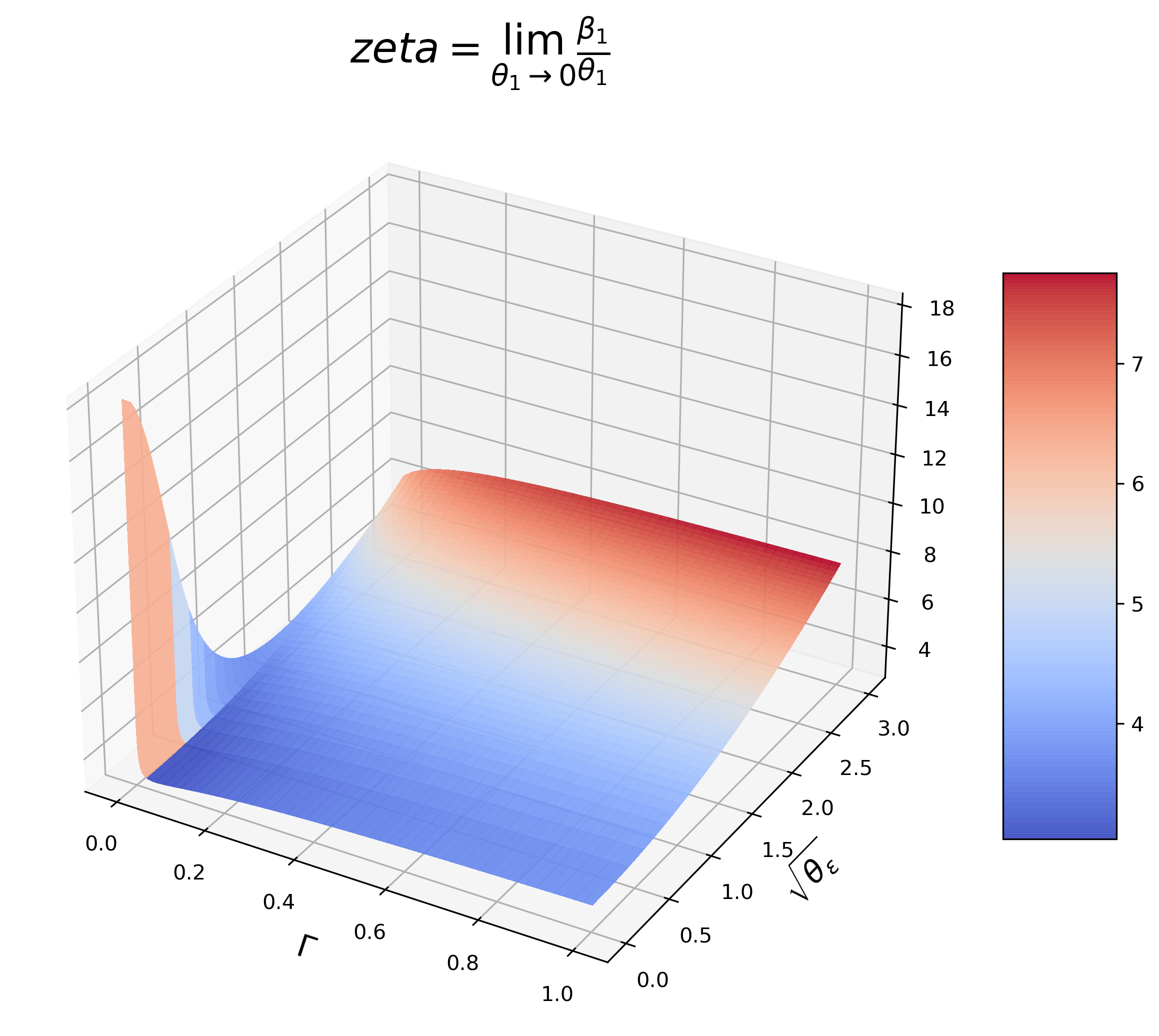
(a) $\Gamma\in[0,1].$

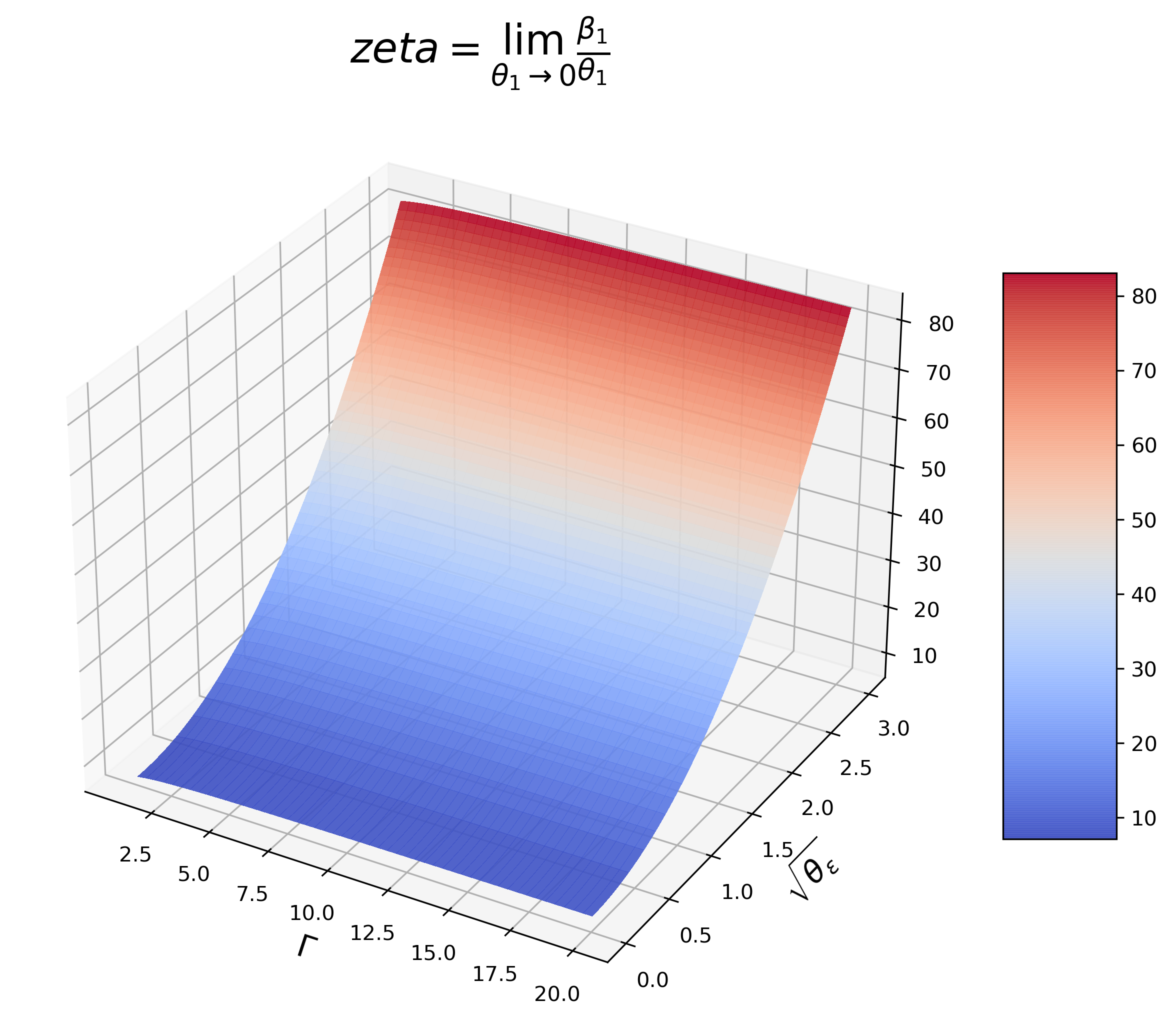
(b) $\Gamma\in[1,20].$

Figure 20: $\zeta(\theta_{\varepsilon},\Gamma),\theta_{\varepsilon}\in[10^{-4},9]$.

Actually, SOC (11) holds only if $|\beta_{23}|<\infty$, i.e., $\lambda_{21}<\infty.$ So when $\theta_{1}\rightarrow 0,$ the equilibrium conditions as $\theta_{1}\rightarrow 0$ are given by

$$\lambda_{22}=\frac{\alpha\sigma_{v}^{2}(1+\beta_{21})}{\alpha^{2}\sigma_{v}^{2}(1+\beta_{21})^{2}+\sigma_{\varepsilon}^{2}\beta_{21}^{2}+\sigma_{2}^{2}},$$ (23)

$$\alpha=\frac{1}{2(\lambda_{22}(1+\beta_{21}))},$$

$$\beta_{21}=\frac{1-\lambda_{22}\alpha}{2(\lambda_{22}+\gamma)}\frac{\alpha\sigma_{v}^{2}}{\alpha\sigma_{v}^{2}+\sigma_{\varepsilon}^{2}},$$

$$\alpha>0,$$

$$\lambda_{22}+\gamma>0.$$

If it is solved, $\{\lambda_{1},\lambda_{21},\beta_{22},\beta_{23}\}$ are given by

$$\lambda_{1}=\alpha\sigma_{v}^{2}\zeta,$$

$$\lambda_{21}=\frac{\alpha\sigma_{v}^{2}(-\beta_{22}(1+\beta_{21})+\sigma_{2}^{2}\zeta-\sigma_{\varepsilon}^{2}\zeta\beta_{21})}{\alpha^{2}\sigma_{v}^{2}(1+\beta_{21})^{2}+\sigma_{\varepsilon}^{2}\beta_{21}^{2}+\sigma_{2}^{2}},$$

$$\beta_{22}=-\frac{\lambda_{21}}{2(\lambda_{22}+\gamma)},$$

$$\beta_{23}=-\frac{\lambda_{21}+2\gamma}{2(\lambda_{22}+\gamma)}.$$

Further simplify three equations in (23), we find that $\beta_{21}$ satisfies (17). We denote the RHS of Equation (17) $f(\beta_{21}),$ when $\theta_{\varepsilon}>0$ or $0<\Gamma<\infty,$ we have

$$f(0)<0,f(\infty)>0,$$

$$f^{\prime}(\beta_{21})>0,\forall\beta_{21}>0.$$

so there must exist a unique $\beta_{21}>0$, such that $f(\beta_{21})=0$.

In the limit, $\mathbb{E}(\pi^{\text{IT}})<\frac{\sigma_{2}\sigma_{v}}{2}$ if and only if

$$\beta_{21}^{2}(\theta_{\varepsilon}-1)<2\beta_{21},$$ (24)

which holds for $\theta_{\varepsilon}\leq 1.$ When $\theta_{\varepsilon}>1,$

$$f(\frac{2}{\theta_{\varepsilon}-1})=\frac{3\theta_{\varepsilon}^{2}-2\theta_{\varepsilon}-1+8\Gamma(\theta_{\varepsilon}^{2}+2\theta_{\varepsilon}+8)}{2(\theta_{\varepsilon}-1)(\theta_{\varepsilon}+1)(\theta_{\varepsilon}-1+2\Gamma(\theta_{\varepsilon}+1))}>0,$$

(24) holds.

References

- [1] Securities, Exchange Commission, et al. Concept release on equity market structure, release no. 34-61358; file no. Technical report, S7-02-10, 2010.
- [2] Liyan Yang and Haoxiang Zhu. Back-running: Seeking and hiding fundamental information in order flows. The Review of Financial Studies, 33(4):1484–1533, 2020.
- [3] Nicholas Hirschey. Do high-frequency traders anticipate buying and selling pressure? Management Science, 67(6):3321–3345, 2021.
- [4] Terrence Hendershott, Charles M Jones, and Albert J Menkveld. Does algorithmic trading improve liquidity? The Journal of finance, 66(1):1–33, 2011.
- [5] Alain P Chaboud, Benjamin Chiquoine, Erik Hjalmarsson, and Clara Vega. Rise of the machines: Algorithmic trading in the foreign exchange market. The Journal of Finance, 69(5):2045–2084, 2014.
- [6] Jonathan Brogaard, Björn Hagströmer, Lars Nordén, and Ryan Riordan. Trading fast and slow: Colocation and liquidity. The Review of Financial Studies, 28(12):3407–3443, 2015.
- [7] Andrei Kirilenko, Albert S. Kyle, Mehrdad Samadi, and Tugkan Tuzun. The flash crash: High frequency trading in an electronic market. The Journal of Finance, 72(3), 2017.
- [8] Markus K Brunnermeier and Lasse Heje Pedersen. Predatory trading. The Journal of Finance, 60(4):1825–1863, 2005.
- [9] Robert A Korajczyk and Dermot Murphy. High-frequency market making to large institutional trades. The Review of Financial Studies, 32(3):1034–1067, 2019.
- [10] Hendrik Bessembinder, Allen Carrion, Laura Tuttle, and Kumar Venkataraman. Liquidity, resiliency and market quality around predictable trades: Theory and evidence. Journal of Financial Economics, 121(1):142–166, 2016.
- [11] Dermot P Murphy and Ramabhadran S Thirumalai. Short-term return predictability and repetitive institutional net order activity. Journal of Financial Research, 40(4):455–477, 2017.
- [12] Søren Bundgaard Brøgger. The market impact of predictable flows: Evidence from leveraged VIX products. Journal of Banking & Finance, 133:106280, 2021.
- [13] Lei Yan, Scott H Irwin, and Dwight R Sanders. Sunshine vs. predatory trading effects in commodity futures markets: New evidence from index rebalancing. Journal of Commodity Markets, 26:100195, 2022.
- [14] Albert S Kyle. Continuous auctions and insider trading. Econometrica: Journal of the Econometric Society, pages 1315–1335, 1985.
- [15] Mehmet Sağlam. Order anticipation around predictable trades. Financial Management, 49(1):33–67, 2020.
- [16] Jonathan Brogaard, Terrence Hendershott, and Ryan Riordan. High-frequency trading and price discovery. The Review of Financial Studies, 27(8):2267–2306, 2014.
- [17] Wei Li. High frequency trading with speed hierarchies. Available at SSRN 2365121, 2018.
- [18] Menkveld and J. Albert. High frequency trading and the new-market makers. Journal of Financial Markets, 16(4):712–740, 2013.
- [19] Ioanid Roşu. Fast and slow informed trading. Journal of Financial Markets, 43:1–30, 2019.
- [20] Peter Hoffmann. A dynamic limit order market with fast and slow traders. Journal of Financial Economics, 113(1):156–169, 2014.
- [21] Thierry Foucault, Johan Hombert, and Ioanid Roşu. News trading and speed. The Journal of Finance, 71(1):335–382, 2016.
- [22] Markus Baldauf and Joshua Mollner. High-frequency trading and market performance. The Journal of Finance, 75(3):1495–1526, 2020.
- [23] Albert J Menkveld. The economics of high-frequency trading: Taking stock. Annual Review of Financial Economics, 8:1–24, 2016.
- [24] Bruce Ian Carlin, Miguel Sousa Lobo, and S Viswanathan. Episodic liquidity crises: Cooperative and predatory trading. The Journal of Finance, 62(5):2235–2274, 2007.
- [25] Torsten Schöneborn and Alexander Schied. Liquidation in the face of adversity: stealth vs. sunshine trading. In EFA 2008 Athens Meetings Paper, 2009.
- [26] Dan Bernhardt and Bart Taub. Front-running dynamics. Journal of Economic Theory, 138(1):288–296, 2008.
- [27] Sebastian Herrmann, Johannes Muhle-Karbe, Dapeng Shang, and Chen Yang. Inventory management for high-frequency trading with imperfect competition. SIAM Journal on Financial Mathematics, 11(1):1–26, 2020.
- [28] Dan Bernhardt and Jianjun Miao. Informed trading when information becomes stale. The Journal of Finance, 59(1):339–390, 2004.
- [29] S. Huddart, J. S. Hughes, and C. B. Levine. Public disclosure and dissimulation of insider trades. Econometrica, 69(3):665–681, 2001.
- [30] Ziyi Xu and Xue Cheng. Are large traders harmed by front-running HFTs? Available at SSRN 4274653, 2022.
- [31] David A Cox, John Little, and Donal O’shea. Using algebraic geometry, volume 185. Springer Science & Business Media, 2006.