An FPTAS for Budgeted Laminar Matroid Independent Set

Abstract

We study the budgeted laminar matroid independent set problem. The input is a ground set, where each element has a cost and a non-negative profit, along with a laminar matroid over the elements and a budget. The goal is to select a maximum profit independent set of the matroid whose total cost is bounded by the budget. Several well known special cases, where we have, e.g., no matroid constraint (the classic knapsack problem) or a uniform matroid constraint (knapsack with a cardinality constraint), admit a fully polynomial-time approximation scheme (FPTAS). In contrast, the budgeted matroid independent set (BMI) problem with a general matroid has an efficient polynomial-time approximation scheme (EPTAS) but does not admit an FPTAS. This implies an EPTAS for our problem, which is the best known result prior to this work.

We present an FPTAS for budgeted laminar matroid independent set, improving the previous EPTAS for this matroid family and generalizing the FPTAS known for knapsack with a cardinality constraint and multiple-choice knapsack. Our scheme is based on a simple dynamic program which utilizes the tree-like structure of laminar matroids.

1 Introduction

Knapsack is one of the most fundamental problems in combinatorial optimization, which has been continuously studied in the past half century. [14, 24, 20, 3]. Considerable attention was given to a generalization of knapsack including an additional matroid constraint [22, 4, 25, 23, 28, 1, 21, 10]. In this work we consider the knapsack problem with a laminar matroid constraint.

A matroid is a set system $(S,{\mathcal{I}})$, where $S$ is a finite set and ${\mathcal{I}}\subseteq 2^{S}$ such that (i) $\emptyset\in{\mathcal{I}}$, (ii) for all $A\in{\mathcal{I}}$ and $B\subseteq A$ it holds that $B\in{\mathcal{I}}$, and (iii) for all $A,B\in{\mathcal{I}}$ where $|A|>|B|$ there is $e\in A\setminus B$ such that $B\cup\{e\}\in{\mathcal{I}}$. We focus on the family of laminar matroids, defined below.

Definition 1.1.

Given a finite set $S$, ${\mathcal{F}}\subseteq 2^{S}\setminus\{\emptyset\}$ is a laminar family on $S$ if for any $X,Y\in{\mathcal{F}}$ one of the following holds: $X\cap Y=\emptyset$, or $X\cap Y=X$, or $X\cap Y=Y$.

Definition 1.2.

Let ${\mathcal{F}}$ be a laminar family on a finite set $S$; also, let $k:{\mathcal{F}}\rightarrow\mathbb{N}_{>0}$ and ${\mathcal{I}}_{{\mathcal{F}},k}=\{A\subseteq S~{}:~{}|A\cap X|\leq k(X)~{}\forall X\in{\mathcal{F}}\}$. Then $(S,{\mathcal{I}}_{{\mathcal{F}},k})$ is a laminar matroid.

The independent sets ${\mathcal{I}}_{{\mathcal{F}},k}$ in the laminar matroid $(S,{\mathcal{I}}_{{\mathcal{F}},k})$ are all subsets of elements $A$ such that for any set $X\in{\mathcal{F}}$ in the laminar family, $|A\cap X|$ does not violate the cardinality constraint $k(X)$. It is well known (see, e.g., [19, 13]) that laminar matroids are indeed matroids.

In this paper, we study the budgeted laminar matroid independent set (BLM) problem. The input is a tuple $I=(S,{\mathcal{F}},k,c,p,B)$, where $S$ is a finite set, ${\mathcal{F}}$ is a laminar family on $S$ such that $S\in{\mathcal{F}}$, $k:{\mathcal{F}}\rightarrow\mathbb{N}_{>0}$ gives cardinality bounds to ${\mathcal{F}}$, $c:S\rightarrow\mathbb{N}$ is a cost function, $p:S\rightarrow\mathbb{N}$ is a profit function, and $B\in\mathbb{N}$ is a budget. A solution of $I$ is an independent set $T\in{\mathcal{I}}_{{\mathcal{F}},k}$ of the laminar matroid $(S,{\mathcal{I}}_{{\mathcal{F}},k})$ such that $c(T)=\sum_{e\in T}c(e)\leq B$. The goal is to find a solution $T$ of $I$ such that $p(T)=\sum_{e\in T}p(e)$ is maximized.

There are a few notable special cases of BLM; we use our notation to formally define them. Consider an instance $I$ of BLM. If ${\mathcal{F}}\setminus\{S\}$ is a partition of $S$ and $k(S)\geq|S|$ then $(S,{\mathcal{I}}_{{\mathcal{F}},k})$ is a partition matroid, and we say that $I$ is a knapsack with partition matroid instance. Moreover, the special case of knapsack with partition matroid where $k(X)=1~{}\forall X\in({\mathcal{F}}\setminus\{S\})$ is the multiple-choice knapsack [28]. Alternatively, if ${\mathcal{F}}=\{S\}$ then $(S,{\mathcal{I}}_{{\mathcal{F}},k})$ is a uniform matroid, and $I$ is a cardinality constrained knapsack instance [22].

A natural application of BLM arises in the context of cloud computing, where limited network bandwidth limit plays a vital role (see, e.g., [29, 27, 26]). Consider a network $G=(V,E)$, that is a directed tree with a root $M$ associated with a cloud computer. Each leaf in $G$ represents a client. Each client sends a job to $M$, which can process the job and broadcast the results through the network back to the client. The jobs have processing times and values. Also, $M$ has a bound on the total processing time of admitted jobs. Moreover, each node $v\in V$ in the network has a limited bandwidth, $k(v)$, so that $v$ can broadcast the results of at most $k(v)$ jobs to its descendant clients. The goal is to maximize the total value of complete jobs subject to the processing time and bandwidth bounds.

We can cast this problem as a BLM instance by taking the set of elements $S$ to be the se of jobs, where the profit and cost of each element are the value and processing time of the corresponding job. Now, we define a laminar family ${\mathcal{F}}$ on the set of elements, where for each vertex $v\in V$ there is a set $X_{v}\in{\mathcal{F}}$ containing all jobss that belong to clients (i.e., leaves) in the subtree rooted by $v$, where the cardinality bound of $X_{v}$ is the bandwidth limit $k(X_{v})=k(v)$. For other applications of laminar matroids, see e.g., [13, 15, 19].

We focus in this paper on approximation schemes for BLM. Let $\textnormal{OPT}(I)$ be the value of an optimal solution for an instance $I$ of a maximization problem $\Pi$. For $\alpha\in(0,1]$, we say that ${\mathcal{A}}$ is an $\alpha$-approximation algorithm for $\Pi$ if, for any instance $I$ of $\Pi$, ${\mathcal{A}}$ outputs a solution of value at least $\alpha\cdot\textnormal{OPT}(I)$. A polynomial-time approximation scheme (PTAS) for $\Pi$ is a family of algorithms $(A_{{\varepsilon}})_{{\varepsilon}>0}$ such that, for any ${\varepsilon}>0$, $A_{{\varepsilon}}$ is a polynomial-time $(1-{\varepsilon})$-approximation algorithm for $\Pi$. An efficient PTAS (EPTAS) is a PTAS $(A_{{\varepsilon}})_{{\varepsilon}>0}$ with running time of the form $f\left(\frac{1}{{\varepsilon}}\right)\cdot|I|^{O(1)}$, where $f$ is an arbitrary computable function. The running time of an EPTAS might be impractically high; this motivates the study of the following important subclass of EPTAS: $(A_{{\varepsilon}})_{{\varepsilon}>0}$ is a fully PTAS (FPTAS) if the running time of $A_{{\varepsilon}}$ is of the form ${\left(\frac{|I|}{{\varepsilon}}\right)}^{O(1)}$.

Figure 1: Complexity of knapsack generalizations with various families of matroid constraints.

We note that budgeted independent set with a general matroid constraint admits an EPTAS; however, the existence of an FPTAS was ruled out [11]. In contrast, well known special cases of BLM such as cardinality constrained knapsack [22] and multiple-choice knapsack [28] admit FPTAS. The question whether budgeted independent set admits an FPTAS on other classes of matroids (e.g., laminar, graphic, or linear matroid) remained open.

In this paper we resolve this open question for laminar matroids. Our main result is an FPTAS for BLM, improving upon the existing EPTAS for this family, and generalizing the FPTAS for the special cases of cardinality constrained knapsack and multiple-choice knapsack. Specifically,

Theorem 1.3.

There is an algorithm FPTAS that given a BLM instance $I$ and ${\varepsilon}>0$ finds in time $O\left(|I|^{5}\cdot{\varepsilon}^{-2}\right)$ a solution $T$ for $I$ of profit $p(T)\geq(1-{\varepsilon})\cdot\textnormal{OPT}(I)$.

We give in Figure 1 a complexity overview of the related problems. To derive an FPTAS, we first find a pseudo-polynomial time algorithm for BLM. Our technique is based on dynamic programming (DP), which exploits the tree-like structure of laminar matroids. More concretely, let $I=(S,{\mathcal{F}},k,c,p,B)$ be a BLM instance and $X\in{\mathcal{F}}$ a maximal set in the laminar family, not contained in any other set except for $S$. We first construct (recursively) DP tables for elements contained in $X$ and separately for elements contained in $S\setminus X$. Then, we combine the two DP tables into a DP table for the original instance $I$. We rely on the key property that combining any two independent sets $T_{1}\subseteq X$ and independent set $T_{2}\subseteq S\setminus X$ yields an independent set $T_{1}\cup T_{2}$ as long as the overall cardinality (i.e., $|T_{1}\cup T_{2}|$) satisfies the cardinality bound of $S$. Finally, our FPTAS is obtained by standard rounding of the profits. We remark that we did not attempt to optimize the running time; instead, our goal is to obtain a simple FPTAS for the problem.

1.1 Related Work

BLM is an immediate generalization of the classic $0/1$-knapsack problem. While the knapsack problem is known to be NP-hard, it admits an FPTAS. Other notable special cases of BLM that admit an FPTAS include cardinality constrained knapsack [22, 4, 25, 23] and multiple choice knapsack [28, 1, 21].

Chakaravarthy et al. [5] considered the knapsack cover with a matroid constraint (KCM) problem, which is dual to budgeted matroid independent set. In this variant, we are given a matroid ${\mathcal{M}}=(S,{\mathcal{I}})$, a cost function $c:S\rightarrow\mathbb{R}_{\geq 0}$, a size function $s:S\rightarrow\mathbb{R}_{\geq 0}$, and a demand $D\in\mathbb{R}_{\geq 0}$. The goal is to find $A\in{\mathcal{I}}$ such that $s(A)=\sum_{e\in A}s(e)\geq D$ such that $c(A)=\sum_{e\in A}c(e)$ is minimized. They obtain a PTAS for a general matroid ${\mathcal{M}}$, and an FPTAS when ${\mathcal{M}}$ is a partition matroid. The constrained minimum spanning tree problem is a special case of KCM where $(S,{\mathcal{I}})$ is a graphic matroid. The constrained minimum spanning tree problem admits an EPTAS [17] and an FPTAS which violates the budget constraint by a factor of $(1+{\varepsilon})$ [18].

As BLM is a special case of the budgeted matroid independent set problem, a PTAS for the problem follows from the works of [16, 6, 2]. An EPTAS for BMI was recently presented in [10] and generalized for budgeted matroid intersection in [9]. As shown in [11], this is the best possible.

1.2 Organization of the Paper

Section 2 gives preliminary results and notations. In Section 3 we give a pseudo-polynomial time algorithm for BLM. Section 4 presents our FPTAS. We conclude in Section 5 with a discussion.

2 Preliminaries

Given a set $S$, a function $f:S\rightarrow\mathbb{N}$, and $R\subseteq S$, let $f(R)=\sum_{e\in R}f(e)$. Also, we sometimes use $f$ to denote a restriction of $f$ to a subset of the domain $S^{\prime}\subseteq S$. Let $I=(S,{\mathcal{F}},k,c,p,B)$ be a BLM instance; we use ${\mathcal{I}}(I)={\mathcal{I}}_{{\mathcal{F}},k}$ to denote the independent sets of the instance. For some $G\subseteq S$ define ${\mathcal{F}}_{\subseteq G}=\{Y\in{\mathcal{F}}~{}|~{}Y\subseteq G\}$ as all sets in ${\mathcal{F}}$ that are contained in $G$. We define below operations on $I$, generating modified BLM instances. We say that a set $X\in{\mathcal{F}}\setminus\{S\}$ is a maximal set if it is not contained in any other set in ${\mathcal{F}}\setminus\{S\}$. For a maximal set $X\in{\mathcal{F}}\setminus\{S\}$, define the BLM instances $I\cap X=(X,{\mathcal{F}}_{\subseteq X},k,c,p,B)$ and $I\setminus X=\big{(}S\setminus X,{\mathcal{F}}_{\subseteq(S\setminus X)}\cup\{S\setminus X\},\bar{k},c,p,B\big{)}$ such that for all $Y\in{\mathcal{F}}_{\subseteq(S\setminus X)}\cup\{S\setminus X\}$

$$\bar{k}(Y)=\begin{cases}k(Y)~{}~{}&Y\in{\mathcal{F}}\\ k(S),~{}~{}&\textnormal{otherwise}.\end{cases}$$

Note that the only set $Y$ that potentially does not belong to ${\mathcal{F}}$ is $Y=S\setminus X$. Observe that $I\cap X$ and $I\setminus X$ can be viewed as restrictions of $I$ to $X$ and $S\setminus X$, respectively. The next observations follow from the above definitions and the properties of laminar families.

Observation 2.1.

For a BLM instance $I=(S,{\mathcal{F}},k,c,p,B)$ and a maximal set $X\in({\mathcal{F}}\setminus\{S\})$ it holds that $I\cap X$ and $I\setminus X$ are BLM instances.

We use $\uplus$ to denote disjoint union.

Observation 2.2.

For a BLM instance $I=(S,{\mathcal{F}},k,c,p,B)$ and a maximal set $X\in({\mathcal{F}}\setminus\{S\})$ the following holds.

1. For any $Q_{1}\in{\mathcal{I}}(I\cap X)$ and $Q_{2}\in{\mathcal{I}}(I\setminus X)$ such that $|Q_{1}\uplus Q_{2}|\leq k(S)$ it holds that $Q_{1}\uplus Q_{2}\in{\mathcal{I}}(I)$.

2. For any $Q\in{\mathcal{I}}(I)$ it holds that $Q\cap X\in{\mathcal{I}}(I\cap X)$ and $Q\setminus X\in{\mathcal{I}}(I\setminus X)$.

3 A Pseudo-polynomial Time Algorithm

In this section we give a pseudo-polynomial time algorithm for BLM. Let $I=(S,{\mathcal{F}},k,c,p,B)$ be a BLM instance, and define $P_{I}=\{0,1,\ldots,|S|\cdot\max_{e\in S}p(e)\}$. Observe that for any solution $T\subseteq S$ it holds that $p(T)\in P_{I}$. Also, there may be $t\in P_{I}$ such that $t\neq p(T)$ for any $T\subseteq S$. Our algorithm computes the following table.

Definition 3.1.

For any BLM instance $I=(S,{\mathcal{F}},k,c,p,B)$, define the DP table of $I$ as the function $\textnormal{{DP}}_{I}:\{0,....|S|\}\times P_{I}\to\mathbb{N}\cup\infty$ such that for all $q\in\{0,1,\ldots,|S|\}$ and $t\in P_{I}$,

$$\textnormal{{DP}}_{I}(q,t)=\min_{Q\in{\mathcal{I}}_{{\mathcal{F}},k}\textnormal{ s.t. }|Q|=q,~{}p(Q)=t}c(Q).$$

For any $q\in\{0,1,\ldots,|S|\}$ and $t\in P_{I}$, the entry $\textsf{DP}_{I}(q,t)$ gives the minimum cost of an independent set in ${\mathcal{I}}_{{\mathcal{F}},k}$ of exactly $q$ elements and profit equal to $t$; if there is no such independent set then $\textsf{DP}_{I}(q,t)=\infty$. Also, $\textsf{DP}_{I}(q,t)=\infty$ if $q$ or $t$ do not belong to the domain of $\textsf{DP}_{I}$ (e.g., $q=|S|+1$).

We formulate a dynamic program which computes the table $\textsf{DP}_{I}$. Informally, the table $\textsf{DP}_{I}$ is constructed by taking a maximal set $X\in{\mathcal{F}}\setminus\{S\}$ in the laminar family (recall that a maximal set is not a subset of any other set in ${\mathcal{F}}\setminus\{S\}$). Our algorithm computes the sub-tables $\textsf{DP}_{I\cap X}$ and $\textsf{DP}_{I\setminus X}$ recursively. An important observation is that the instances $I\cap X$ and $I\setminus X$ are disjoint; thus, the table $\textsf{DP}_{I}$ can be computed from $DP_{I\cap X}$ and $DP_{I\setminus X}$ using a convolution. Specifically, to compute an entry $\textsf{DP}_{I}(q,t)$ for $q\in\{0,1,\ldots,|S|\}$ and $t\in P_{I}$, we find the minimum solution induced by partitioning the values $q$ and $t$ between the complementary sub-instances $I\cap X$ and $I\setminus X$. This is formalized by the next lemma.

Lemma 3.2.

Let $I=(S,{\mathcal{F}},k,c,p,B)$ be a BLM instance, and $X\in{\mathcal{F}}\setminus\{S\}$ a maximal set. Then, for all $q\in\{0,1,\ldots,|S|\}$ and $t\in P_{I}$,

$$\textnormal{{DP}}_{I}(q,t)=\begin{cases}\min_{\begin{subarray}{c}q_{1},q_{2},t_{1},t_{2}\in\mathbb{N}\textnormal{ s.t. }\\ q_{1}+q_{2}=q,~{}t_{1}+t_{2}=t\end{subarray}}\left\{\textnormal{{DP}}_{I\cap X}(q_{1},t_{1})+\textnormal{{DP}}_{I\setminus X}(q_{2},t_{2})\right\}~{}~{}&\textnormal{if}\ q\leq k(S)\\ \infty~{}~{}&\textnormal{otherwise}\end{cases}$$

Proof.

Let $q\in\{0,1,\ldots,|S|\}$ and $t\in P_{I}$. For simplicity, let

$$M=\min_{\begin{subarray}{c}q_{1},q_{2},t_{1},t_{2}\in\mathbb{N}\textnormal{ s.t. }\\ q_{1}+q_{2}=q,~{}t_{1}+t_{2}=t\end{subarray}}\left\{\textnormal{{DP}}_{I\cap X}(q_{1},t_{1})+\textnormal{{DP}}_{I\setminus X}(q_{2},t_{2})\right\}.$$

We first consider the case where $\textnormal{{DP}}_{I}(q,t)$ and $M$ differ from $\infty$. We use the following auxiliary claims.

Claim 3.3.

If $\textnormal{{DP}}_{I}(q,t)\neq\infty$ then $M\leq\textnormal{{DP}}_{I}(q,t)$.

Proof.

As $\textnormal{{DP}}_{I}(q,t)\neq\infty$ there is $Q^{*}\in{\mathcal{I}}_{{\mathcal{F}},k}$ such that

$$Q^{*}=\operatorname*{arg\,min}_{Q\in{\mathcal{I}}_{{\mathcal{F}},k}\textnormal{ s.t. }|Q|=q,~{}p(Q)=t}c(Q).$$ (1)

Let $q^{*}_{1}=|Q^{*}\cap X|,q^{*}_{2}=|Q^{*}\setminus X|,t^{*}_{1}=p(Q^{*}\cap X)$, and $t^{*}_{2}=p(Q^{*}\setminus X)$. By (1), and since $S=X\uplus(S\setminus X)$, it holds that

$$|Q^{*}|=|Q^{*}\cap X|+|Q^{*}\setminus X|=q^{*}_{1}+q^{*}_{2}=q$$

and

$$p(Q^{*})=p(Q^{*}\cap X)+p(Q^{*}\setminus X)=t^{*}_{1}+t^{*}_{2}=t.$$

Moreover, by Observation 2.2, since $Q^{*}\in{\mathcal{I}}_{{\mathcal{F}},k}$, it holds that $Q^{*}\cap X\in{\mathcal{I}}(I\cap X)$ and $Q^{*}\setminus X\in{\mathcal{I}}(I\setminus X)$ . Thus,

$$\textnormal{{DP}}_{I}(q,t)=c(Q^{*})=c(Q^{*}\cap X)+c(Q^{*}\setminus X)\geq\textnormal{{DP}}_{I\cap X}(q^{*}_{1},t^{*}_{1})+\textnormal{{DP}}_{I\setminus X}(q^{*}_{2},t^{*}_{2})\geq M.$$

The first inequality holds since $\textnormal{{DP}}_{I\cap X}(q^{*}_{1},t^{*}_{1})$ is the minimum cost of $Q\in{\mathcal{I}}(I\cap X)$ such that $|Q|=q^{*}_{1}$ and $p(Q)=t^{*}_{1}$; since $Q^{*}\cap X$ satisfies these conditions (by Observation 2.2), we conclude that $c(Q^{*}\cap X)\geq\textnormal{{DP}}_{I\cap X}(q^{*}_{1},t^{*}_{1})$. Similar arguments show that $c(Q^{*}\setminus X)\geq\textnormal{{DP}}_{I\setminus X}(q^{*}_{2},t^{*}_{2})$. The second inequality holds since $M$ is the minimum value of $\textnormal{{DP}}_{I\cap X}(q_{1},t_{1})+\textnormal{{DP}}_{I\setminus X}(q_{2},t_{2})$ over all $q_{1},q_{2},t_{1},t_{2}\in\mathbb{N}$ such that $q_{1}+q_{2}=q,t_{1}+t_{2}=t$. As $q^{*}_{1},q^{*}_{2},t^{*}_{1},t^{*}_{2}\in\mathbb{N}$ and $q^{*}_{1}+q^{*}_{2}=q,t^{*}_{1}+t^{*}_{2}=t$, the inequality follows. $\square$

Claim 3.4.

If $M\neq\infty$ and $q\leq k(S)$ then $\textnormal{{DP}}_{I}(q,t)\leq M$.

Proof.

Let $q^{\prime}_{1},q^{\prime}_{2},t^{\prime}_{1},t^{\prime}_{2}\in\mathbb{N},q^{\prime}_{1}+q^{\prime}_{2}=q,t^{\prime}_{1}+t^{\prime}_{2}=t$ such that

$$\textnormal{{DP}}_{I\cap X}(q^{\prime}_{1},t^{\prime}_{1})+\textnormal{{DP}}_{I\setminus X}(q^{\prime}_{2},t^{\prime}_{2})=M.$$

Since $M\neq\infty$, there exist

$$Q^{\prime}_{1}=\operatorname*{arg\,min}_{Q\in{\mathcal{I}}(I\cap X)\textnormal{ s.t. }|Q|=q^{\prime}_{1},~{}p(Q)=t^{\prime}_{1}}c(Q),~{}~{}~{}~{}~{}~{}~{}~{}~{}~{}~{}~{}~{}~{}~{}~{}~{}Q^{\prime}_{2}=\operatorname*{arg\,min}_{Q\in{\mathcal{I}}(I\setminus X)\textnormal{ s.t. }|Q|=q^{\prime}_{2},~{}p(Q)=t^{\prime}_{2}}c(Q).$$ (2)

By (2),

$$M={} \textnormal{{DP}}_{I\cap X}(q^{\prime}_{1},t^{\prime}_{1})+\textnormal{{DP}}_{I\setminus X}(q^{\prime}_{2},t^{\prime}_{2})$$

$$={} c(Q^{\prime}_{1})+c(Q^{\prime}_{2})$$

$$={} c(Q^{\prime}_{1}\uplus Q^{\prime}_{2})$$

$$\geq{} \min_{Q\in{\mathcal{I}}_{{\mathcal{F}},k}\textnormal{ s.t. }|Q|=q,~{}p(Q)=t}c(Q)$$

$$={} \textsf{DP}_{I}(q,t).$$

The above inequality follows from the next arguments. As $q^{\prime}_{1}+q^{\prime}_{2}=q$ and $q\leq k(S)$, by Observation 2.2 $Q^{\prime}_{1}\uplus Q^{\prime}_{2}\in{\mathcal{I}}_{{\mathcal{F}},k}$; also, $|Q^{\prime}_{1}\uplus Q^{\prime}_{2}|=q$, and $p(Q^{\prime}_{1}\uplus Q^{\prime}_{2})=t^{\prime}_{1}+t^{\prime}_{2}=t$. The inequality follows, as the minimum in the right-hand side of the inequality considers $Q=Q^{\prime}_{1}\uplus Q^{\prime}_{2}$ in particular. $\square$

To complete the proof of the lemma, we consider four complementary cases.

• If $q>k(S)$ then $\textsf{DP}_{I}(q,t)=\infty$ by Definition 3.1.

• If $M=\infty$ then $\textsf{DP}_{I}(q,t)=\infty$ by Claim 3.3.

• If $q\leq k(S)$ and $\textsf{DP}_{I}(q,t)=\infty$ then by Claim 3.4 $M=\infty$ .

• If $q\leq k(S)$ and $\textsf{DP}_{I}(q,t)\neq\infty$ then, by Claims 3.3 and 3.4, $\textsf{DP}_{I}(q,t)=M$.

∎

Note that computing the table $\textsf{DP}_{I}$ by Lemma 3.2 is possible only if there is a maximal set $X\in{\mathcal{F}}\setminus\{S\}$; this requires more than one set in the laminar family. If $|{\mathcal{F}}|=1$, we compute the table $\textsf{DP}_{I}$ using two alternative ways, depending on whether $|S|=1$ or $|S|>1$. The next observation considers the case where the instance consists of a single element; it follows immediately from Definition 3.1.

Observation 3.5.

For a BLM instance $I=(S,{\mathcal{F}},k,c,p,B)$ such that $|S|=1$ it holds that $\textnormal{{DP}}_{I}(1,p(S))=c(S)$, $\textnormal{{DP}}_{I}(0,0)=0$, and for any other $(q,t)\in\{0,\ldots,|S|\}\times P_{I}$ it holds that $\textnormal{{DP}}_{I}(q,t)=\infty$.

We now consider the case where $|S|>1$ and ${\mathcal{F}}=\{S\}$. Here, we define a new instance which adds a (redundant) partition of S into two subsets. This partition allows us to use the recursive computation as given in Lemma 3.2. For a BLM instance $I=(S,{\mathcal{F}},k,c,p,B)$ such that ${\mathcal{F}}=\{S\}$ and $|S|>1$, we say that the BLM instance $\tilde{I}=(S,\tilde{{\mathcal{F}}},\tilde{k},c,p,B)$ is a partitioned-instance of $I$ if the following holds.

• $\tilde{{\mathcal{F}}}=\{S_{1},S_{2},S\}$ where $S_{1},S_{2}$ is a partition of $S$.

• $\tilde{k}:\tilde{{\mathcal{F}}}\rightarrow\mathbb{N}$ and $\tilde{k}(S_{1})=\tilde{k}(S_{2})=\tilde{k}(S)=k(S)$.

Note that $S_{1},S_{2}\neq\emptyset$ since $|S|>1$. The next lemma states that the independent sets of an instance $I$ and of a partitioned-instance of $I$ are identical.

Lemma 3.6.

For any BLM instance $I=(S,{\mathcal{F}},k,c,p,B)$ such that ${\mathcal{F}}=\{S\}$ and $|S|>1$, and a partitioned-instance $\tilde{I}=(S,\tilde{{\mathcal{F}}},\tilde{k},c,p,B)$ of $I$ it holds that ${\mathcal{I}}_{{\mathcal{F}},k}={\mathcal{I}}_{\tilde{{\mathcal{F}}},\tilde{k}}$.

Proof.

Let $\tilde{{\mathcal{F}}}=\{S_{1},S_{2},S\}$ and $Q\in{\mathcal{I}}_{{\mathcal{F}},k}$. Then $|Q|\leq k(S)=\tilde{k}(S)$, and

$$|Q\cap S_{1}|\leq|Q|\leq k(S)=\tilde{k}(S_{1}).$$

Similarly, $|Q\cap S_{2}|\leq\tilde{k}(S_{2})$. Thus, $Q\in{\mathcal{I}}_{\tilde{{\mathcal{F}}},\tilde{k}}$. For the other direction, let $\tilde{Q}\in{\mathcal{I}}_{\tilde{{\mathcal{F}}},\tilde{k}}$. Then, $|\tilde{Q}|\leq\tilde{k}(S)=k(S)$ and it follows that $\tilde{Q}\in{\mathcal{I}}_{{\mathcal{F}},k}$. We conclude that ${\mathcal{I}}_{{\mathcal{F}},k}={\mathcal{I}}_{\tilde{{\mathcal{F}}},\tilde{k}}$. ∎

The next result follows immediately from Lemma 3.6 and Definition 3.1.

Corollary 3.7.

For any BLM instance $I$ such that ${\mathcal{F}}=\{S\}$ and $|S|>1$, and a partitioned-instance $\tilde{I}$ of $I$, it holds that $\textnormal{{DP}}_{\tilde{I}}=\textnormal{{DP}}_{I}$.

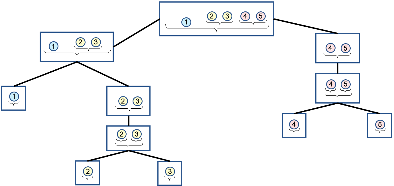
Figure 2: An illustration of the recursive calls of Algorithm 1 for a BLM instance $I$ with five elements $S=\{1,2,3,4,5\}$, represented by the circles. The underbraces indicate the sets in the laminar family ${\mathcal{F}}$ of the instance in each node of the tree. For example, in the root node, ${\mathcal{F}}=\{S,\{2,3\},\{4,5\}\}$.

Using the above, we derive a pseudo-polynomial time algorithm which computes $\textsf{DP}_{I}$. If there is one element, the algorithm computes $\textsf{DP}_{I}$ using Observation 3.5; otherwise, if there is one set ${\mathcal{F}}=\{S\}$ in the laminar family, the algorithm computes $\textsf{DP}_{I}$ by a recursive call to the algorithm with a partitioned-instance. The remaining case is that there exists a maximal set $X\in{\mathcal{F}}\setminus\{S\}$ for which we can apply the recursive computation of the table via Lemma 3.2. We give an illustration of recursive calls the algorithm initiates in Figure 2. The pseudocode of the algorithm is given in Algorithm 1. For a BLM instance $I$, we use $d(I)$ to denote the recursion depth in the execution of $\textsf{ComputeDP}\left(I\right)$.

1

input :  A BLM instance $I=(S,{\mathcal{F}},k,c,p,B)$.

2

output : The table $\textsf{DP}_{I}$ as defined in Definition 3.1.

3

4Initialize $\textnormal{{DP}}_{I}(q,t)=\infty$ for all $q\in\{0,1,\ldots,|S|\}$ and $t\in P_{I}$.

5if $|S|=1$ then

6      

7      Set $\textnormal{{DP}}_{I}(1,p(S))\leftarrow c(S)$ and $\textnormal{{DP}}_{I}(0,0)\leftarrow 0$.

8      Return the table $\textnormal{{DP}}_{I}$.

9 end if

10

11if $|{\mathcal{F}}|=1$ then

12      

13      Return $\textsf{ComputeDP}\left(\tilde{I}\right)$ where $\tilde{I}$ is a partitioned-instance of $I$.

14 end if

15

16Find a maximal set $X\in{\mathcal{F}}\setminus\{S\}$ .

17Compute $\textsf{DP}_{I\cap X}\leftarrow\textsf{ComputeDP}(I\cap X)$ and $\textsf{DP}_{I\setminus X}\leftarrow\textsf{ComputeDP}(I\setminus X)$.

18For $q\in\{0,1,\ldots,|S|\}$ and $t\in P_{I}$ set

$$\textnormal{{DP}}_{I}(q,t)=\begin{cases}\min_{\begin{subarray}{c}q_{1},q_{2},t_{1},t_{2}\in\mathbb{N}\textnormal{ s.t. }\\ q_{1}+q_{2}=q,t_{1}+t_{2}=t\end{subarray}}\left\{\textnormal{{DP}}_{I\cap X}(q_{1},t_{1})+\textnormal{{DP}}_{I\setminus X}(q_{2},t_{2})\right\}~{}~{}&\textnormal{if}\ q\leq k(S)\\ \infty~{}~{}&\textnormal{otherwise}\end{cases}$$

Return the table $\textnormal{{DP}}_{I}$.

Algorithm 1 $\textsf{ComputeDP}(I)$

Lemma 3.8.

For any BLM instance $I=(S,{\mathcal{F}},k,c,p,B)$ Algorithm 1 returns the table $\textnormal{{DP}}_{I}$.

Proof.

We show that for every BLM instance $I=(S,{\mathcal{F}},k,c,p,B)$ it holds that $\textsf{ComputeDP}\left(I\right)=\textsf{DP}_{I}$. The proof is by induction on $d(I)$. For the base case, let $I$ be a BLM instance such that $d(I)=1$. Then, it holds that $|S|=1$ and the algorithm returns $\textsf{DP}_{I}$ by Observation 3.5 and Steps 1, 1 of Algorithm 1. For some $n\in\mathbb{N}_{>0}$, assume that for every BLM instance $I^{\prime}$ for which $d(I^{\prime})\leq n$, it holds that $\textsf{ComputeDP}\left(I^{\prime}\right)=\textsf{DP}_{I^{\prime}}$. For the induction step, let $I=(S,{\mathcal{F}},k,c,p,B)$ be a BLM instance such that $d(I)=n+1$. We consider two cases.

1. $|{\mathcal{F}}|=1$. Then Algorithm 1 returns $\textsf{ComputeDP}\left(\tilde{I}\right)$ by Step 1, where $\tilde{I}$ is a partitioned-instance of $I$. By the induction hypothesis, it holds that $\textsf{ComputeDP}\left(\tilde{I}\right)=\textsf{DP}_{\tilde{I}}$. Thus, by Corollary 3.7, we have $\textsf{ComputeDP}\left(I\right)=\textsf{ComputeDP}\left(\tilde{I}\right)=\textsf{DP}_{I}$.

2. $|{\mathcal{F}}|>1$. In Step 1 in the (non-recursive) computation of $\textsf{ComputeDP}\left(I\right)$, the algorithm finds a maximal set $X\in{\mathcal{F}}\setminus\{S\}$. By the assumption of the induction it follows that $\textsf{ComputeDP}(I\cap X)=\textsf{DP}_{I\cap X}$ and $\textsf{ComputeDP}(I\setminus X)=\textsf{DP}_{I\setminus X}$. Therefore, by Step 18 and Lemma 3.2 it holds that $\textsf{ComputeDP}\left(I\right)=\textsf{DP}_{I}$.

∎

For the running time of Algorithm 1, assume that the laminar family is represented by a linked list of sets, and that the elements in each set are represented by a bit map.

Lemma 3.9.

For any BLM instance $I=(S,{\mathcal{F}},k,c,p,B)$, the running time of Algorithm 1 on $I$ is $O(|S|^{3}\cdot|P_{I}|^{2})$.

Proof.

We use the next claim.

Claim 3.10.

For any BLM instance $I=(S,{\mathcal{F}},k,c,p,B)$, Algorithm 1 makes at most $3\cdot|S|$ recursive calls during the execution of $\textnormal{{ComputeDP}}(I)$.

Proof.

Consider the tree of recursive calls generated throughout the execution of $\textnormal{{ComputeDP}}(I)$. Each element in $S$ has a unique leaf in the tree; therefore, the number of leaves is bounded by $|S|$. Moreover, since there are $|S|$ leaves, the number of internal nodes in the tree that have two children is bounded by $|S|-1$; thus, the number of recursive calls initiated in Step 1 is at most $|S|$. Finally, after each recursive call from Step 1 the algorithm applies a recursive call from Step 1. Therefore, the number of recursive calls from Step 1 is at most $|S|$. Overall, Algorithm 1 makes at most $3\cdot|S|$ recursive calls. $\square$

To complete the proof, we show that the running time of the algorithm, excluding the recursive calls, is $O(|S|^{2}\cdot|P_{I}|^{2})$. As the recursive calls in the algorithm use instances in which the number of elements is bounded by $|S|$, and the set of profits is of size at most $P_{I}$, the statement of the lemma follows from Claim 3.10. Computing Step 1 takes $O(|S|\cdot|P_{I}|)$. Moreover, Step 1 can be computed in time $O(|S|)$ using an arbitrary partition of the elements. Step 1 can be computed in time $O(|S|)$ by iterating over all sets in the laminar family ${\mathcal{F}}$. Also, computing each entry in the table $\textsf{DP}_{I}$ in Step 18 takes $O(|S|\cdot|P_{I}|)$; thus, computing the entire table takes $O(|S|^{2}\cdot|P_{I}|^{2})$. Overall, the running time is $O(|S|^{3}\cdot|P_{I}|^{2})$. ∎

4 An FPTAS for BLM

In this section we use the dynamic program in Section 3 to derive an FPTAS for BLM, leading to the proof of Theorem 1.3. Let $I=(S,{\mathcal{F}},k,c,p,B)$ be a BLM instance and let ${\varepsilon}>0$ be an error parameter. Note that the computation time of $\textsf{DP}_{I}$ depends on $|P_{I}|$, may not be polynomial in the input size. To obtain a polynomial-time algorithm, we round down the profit of each item $e$ to $\left\lfloor\frac{p(e)}{\alpha}\right\rfloor$, where $\alpha=\frac{{\varepsilon}\cdot\max_{e\in S}p(e)}{|S|}$. This generates a reduced instance $\bar{I}$, for which the table $\textsf{DP}_{I}$ can be computed efficiently. Then, by iterating over all possible values in $\textsf{DP}_{I}$, we compute the value of the optimum for $\bar{I}$; this gives an almost optimal solution for $I$, where the solution itself is computed using standard backtracking. The pseudocode of the algorithm is given in Algorithm 2.

1

input : A BLM instance $I=(S,{\mathcal{F}},k,c,p,B)$ and an error parameter ${\varepsilon}>0$.

2

output : A solution $T$ of $I$ with profit $p(T)\geq(1-{\varepsilon})\cdot\textnormal{OPT}(I)$.

3

4Let $\alpha\leftarrow\frac{{\varepsilon}\cdot\max_{e\in S}p(e)}{|S|}$ and define $\bar{p}(e)\leftarrow\left\lfloor\frac{p(e)}{\alpha}\right\rfloor~{}\forall e\in S$.

5Compute $\textsf{DP}_{\bar{I}}\leftarrow\textsf{ComputeDP}(\bar{I})$, where $\bar{I}=(S,{\mathcal{F}},k,c,\bar{p},B)$.

6Let $\lambda\leftarrow\bigg{\{}(q,t)\in\{0,\ldots,|S|\}\times P_{\bar{I}}~{}\bigg{|}~{}\textsf{DP}_{\bar{I}}(q,t)\leq B\bigg{\}}$.

Use backtracking to find a solution $T$ for $I$ of value $\max_{(q,t)\in\lambda}t$.

Algorithm 2 $\textsf{FPTAS}(I,{\varepsilon})$

Proof of Theorem 1.3: We show that Algorithm 2 is an FPTAS for BLM. Let $\bar{I}=(S,{\mathcal{F}},k,c,\bar{p},B)$ be the instance with the rounded profits as given in Algorithm 2. By Lemma 3.8, $\textsf{ComputeDP}(\bar{I})$ returns the table $\textsf{DP}_{\bar{I}}$ as given in Definition 3.1. Thus, for all $(q,t)\in\lambda$ there is a solution for $\bar{I}$ of profit $t$ if and only if $\textsf{DP}_{\bar{I}}(q,t)\leq B$. Let $T$ be an optimal solution for $\bar{I}$. By the above, we have

$$\bar{p}(T)=\max_{(q,t)\in\lambda}t=\textnormal{OPT}(\bar{I})$$ (3)

Let $T^{*}$ be an optimal solution of $I$. Then,

$$\bar{p}(T^{*})=\sum_{e\in T^{*}}\left\lfloor\frac{p(e)}{\alpha}\right\rfloor\geq\sum_{e\in T^{*}}\left(\frac{p(e)}{\alpha}-1\right)\geq\sum_{e\in T^{*}}\left(\frac{p(e)}{\alpha}\right)-|S|=\frac{\textnormal{OPT}(I)}{\alpha}-|S|.$$ (4)

Hence,

$$p(T)\geq\alpha\cdot\bar{p}(T)\geq\alpha\cdot\bar{p}(T^{*})\geq\alpha\cdot\left(\frac{\textnormal{OPT}(I)}{\alpha}-|S|\right)=\textnormal{OPT}(I)-{\varepsilon}\cdot\max_{e\in S}p(e)\geq(1-{\varepsilon})\cdot\textnormal{OPT}(I).$$

The first inequality holds by Step 2. The second inequality follows from the optimality of $\bar{p}(T)$ by (3). The third inequality holds by (4). The last inequality holds since $\textnormal{OPT}(I)\geq\max_{e\in S}p(e)$ (assuming that $c(e)\leq B~{}\forall e\in S$).

We now analyze the running time of the scheme. We note that Step 2 takes linear time. The running time of Step 2 is $O(|S|^{3}\cdot|P_{\bar{I}}|^{2})$ by Lemma 3.9. Finally, Steps 2 and 2 can be computed in time $O(|S|\cdot|P_{\bar{I}}|)$ by the definition of $\lambda$. Hence, the overall running time is

$$O\left(|S|^{3}\cdot|P_{\bar{I}}|^{2}\right)=O\left(|I^{5}|\cdot{\varepsilon}^{-2}\right).$$

The equality follows since $|\bar{P}_{\bar{I}}|=O(|S|\cdot{\varepsilon}^{-1})$ by Step 2. $\blacksquare$

5 Discussion

In this paper we showed that the budgeted laminar matroid independent set (BLM) problem admits an FPTAS, thus improving upon the existing EPTAS for this matroid family, and generalizing the FPTAS for the special cases of cardinality constrained knapsack and multiple-choice knapsack. Our FPTAS is based on a natural dynamic program which utilizes the tree-like structure of laminar matroids. It seems that with slight modifications our scheme yields an FPTAS for the more general problem of budgeted $k$-laminar matroid independent set, where $k\in\mathbb{N}$ is fixed.

An intriguing open question is whether BMI admits an FPTAS on other families of matroids, such as graphic matroids, transversal matroids, or linear matroids.

We note that the running time of our scheme is $O(|I|^{5}\cdot{\varepsilon}^{-2})$, whereas the running time of the state of the art FPTAS for knapsack is $O(|I|+{\varepsilon}^{-2.2})$ [8], which almost matches the lower bound of $\tilde{O}\left((|I|+{\varepsilon}^{-1})^{2-o(1)}\right)$ for the problem [7]. It would be interesting to design an FPTAS for BLM that matches the running time of [8], or to obtain a stronger lower bound for this problem.

References

• [1] Bansal, M., Venkaiah, V.: Improved fully polynomial time approximation scheme for the 0-1 multiple-choice knapsack problem. International Institute of Information Technology Tech Report pp. 1–9 (2004)
• [2] Berger, A., Bonifaci, V., Grandoni, F., Schäfer, G.: Budgeted matching and budgeted matroid intersection via the gasoline puzzle. Mathematical Programming 128(1), 355–372 (2011)
• [3] Cacchiani, V., Iori, M., Locatelli, A., Martello, S.: Knapsack problems-an overview of recent advances. part ii: Multiple, multidimensional, and quadratic knapsack problems. Computers & Operations Research p. 105693 (2022)
• [4] Caprara, A., Kellerer, H., Pferschy, U., Pisinger, D.: Approximation algorithms for knapsack problems with cardinality constraints. European Journal of Operational Research 123(2), 333–345 (2000)
• [5] Chakaravarthy, V.T., Choudhury, A.R., Natarajan, S.R., Roy, S.: Knapsack cover subject to a matroid constraint. In: IARCS Annual Conference on Foundations of Software Technology and Theoretical Computer Science (FSTTCS 2013) (2013)
• [6] Chekuri, C., Vondrák, J., Zenklusen, R.: Multi-budgeted matchings and matroid intersection via dependent rounding. In: Proceedings of the twenty-second annual ACM-SIAM symposium on Discrete Algorithms. pp. 1080–1097 (2011)
• [7] Cygan, M., Mucha, M., Wegrzycki, K., Włodarczyk, M.: On problems equivalent to (min,+)-convolution. ACM Transactions on Algorithms (TALG) 15(1), 1–25 (2019)
• [8] Deng, M., Jin, C., Mao, X.: Approximating knapsack and partition via dense subset sums. In: Proceedings of the 2023 Annual ACM-SIAM Symposium on Discrete Algorithms (SODA). pp. 2961–2979 (2023)
• [9] Doron-Arad, I., Kulik, A., Shachnai, H.: An EPTAS for budgeted matching and budgeted matroid intersection. arXiv preprint arXiv:2302.05681 (2023)
• [10] Doron-Arad, I., Kulik, A., Shachnai, H.: An EPTAS for budgeted matroid independent set. In: Symposium on Simplicity in Algorithms (SOSA). pp. 69–83 (2023)
• [11] Doron-Arad, I., Kulik, A., Shachnai, H.: Hardness of weighted matroid problems. Manuscript (2023)
• [12] Fife, T., Oxley, J.: Generalized laminar matroids. European Journal of Combinatorics 79, 111–122 (2019)
• [13] Gabow, H., Kohno, T.: A network-flow-based scheduler: Design, performance history, and experimental analysis. Journal of Experimental Algorithmics (JEA) 6, 3–es (2001)
• [14] Gilmore, P., Gomory, R.E.: The theory and computation of knapsack functions. Operations Research 14(6), 1045–1074 (1966)
• [15] Gourvès, L., Monnot, J., Tlilane, L.: Worst case compromises in matroids with applications to the allocation of indivisible goods. Theoretical Computer Science 589, 121–140 (2015)
• [16] Grandoni, F., Zenklusen, R.: Approximation schemes for multi-budgeted independence systems. In: European Symposium on Algorithms. pp. 536–548 (2010)
• [17] Hassin, R., Levin, A.: An efficient polynomial time approximation scheme for the constrained minimum spanning tree problem using matroid intersection. SIAM Journal on Computing 33(2), 261–268 (2004)
• [18] Hong, S.P., Chung, S.J., Park, B.H.: A fully polynomial bicriteria approximation scheme for the constrained spanning tree problem. Operations Research Letters 32(3), 233–239 (2004)
• [19] Im, S., Wang, Y.: Secretary problems: Laminar matroid and interval scheduling. In: Proceedings of the twenty-second annual ACM-SIAM symposium on Discrete Algorithms. pp. 1265–1274 (2011)
• [20] Kellerer, H., Pferschy, U., Pisinger, D.: Multidimensional knapsack problems. Springer (2004)
• [21] Kellerer, H., Pferschy, U., Pisinger, D.: The multiple-choice knapsack problem. In: Knapsack Problems, pp. 317–347 (2004)
• [22] Knuth, D.E.: Computer Programming as an Art. Commun. ACM 17(12), 667–673 (1974)
• [23] Li, W., Lee, J., Shroff, N.: A faster FPTAS for knapsack problem with cardinality constraint. Discrete Applied Mathematics 315, 71–85 (2022)
• [24] Martello, S., Toth, P.: Knapsack problems: algorithms and computer implementations. John Wiley & Sons, Inc. (1990)
• [25] Mastrolilli, M., Hutter, M.: Hybrid rounding techniques for knapsack problems. Discrete applied mathematics 154(4), 640–649 (2006)
• [26] Popa, L., Kumar, G., Chowdhury, M., Krishnamurthy, A., Ratnasamy, S., Stoica, I.: Faircloud: Sharing the network in cloud computing. In: Proceedings of the ACM SIGCOMM 2012 conference on Applications, technologies, architectures, and protocols for computer communication. pp. 187–198 (2012)
• [27] Popa, L., Yalagandula, P., Banerjee, S., Mogul, J.C., Turner, Y., Santos, J.R.: Elasticswitch: Practical work-conserving bandwidth guarantees for cloud computing. In: Proceedings of the ACM SIGCOMM 2013 conference. pp. 351–362 (2013)
• [28] Sinha, P., Zoltners, A.A.: The multiple-choice knapsack problem. Operations Research 27(3), 503–515 (1979)
• [29] Zhu, J., Li, D., Wu, J., Liu, H., Zhang, Y., Zhang, J.: Towards bandwidth guarantee in multi-tenancy cloud computing networks. In: 2012 20th IEEE International Conference on Network Protocols (ICNP). pp. 1–10 (2012)