Detecting inner-LAN anomalies using hierarchical forecasting

Abstract

Increasing activity and the number of devices online are leading to increasing and more diverse cyber attacks. This continuously evolving attack activity makes signature-based detection methods ineffective. Once malware has infiltrated into a LAN, bypassing an external gateway or entering via an unsecured mobile device, it can potentially infect all nodes in the LAN as well as carry out nefarious activities such as stealing valuable data, leading to financial damage and loss of reputation. Such infiltration could be viewed as an insider attack, increasing the need for LAN monitoring and security. In this paper we aim to detect such inner-LAN activity by studying the variations in Address Resolution Protocol (ARP) calls within the LAN. We find anomalous nodes by modelling inner-LAN traffic using hierarchical forecasting methods. We substantially reduce the false positives ever present in anomaly detection, by using an extreme value theory based method. We use a dataset from a real inner-LAN monitoring project, containing over 10M ARP calls from 362 nodes. Furthermore, the small number of false positives generated using our methods, is a potential solution to the ”alert fatigue” commonly reported by security experts.

Key words— Anomaly detection, Local area networks, Machine learning, Statistical analysis, Time series, hierarchical forecasting, extreme value theory

1 Introduction

As recent events show, data breaches and cyber attacks are becoming ever more common. System administrators are often unaware of infiltrators until after data has been siphoned off. Greater scrutiny within the LAN architecture may help alert system administrators to such infiltration. However, current security architecture does not take this into consideration, with most intrusion and anomaly detection happening only at the gateway. Our paper uses advanced forecasting methods and works with data from a LAN monitoring system to detect anomalies within the LAN. Our focus is on inner-LAN traffic and we have made this inner-LAN dataset comprising over 10M observations available.

Forecasting techniques allow better early detection of abnormal behaviour, such as high number of ARP calls, that may be the result of security breaches. Although forecasting has been used for detecting anomalies in traffic (Cui et al., 2019) and other domains such as power load forecasting (Bernacki and Kołaczek, 2015), applications of hierarchical forecasting to computer security network systems are yet to be investigated. Unlike conventional forecasting methods that investigate a single node, hierarchical forecasting methods leverage information from other nodes in the network to extract information useful for predicting node behaviour. Inspired by the architecture of the LAN, in this paper, we build a hierarchical time series structure and use information from across the network to construct advanced forecasting models that enable detection of anomalies in the network. In the realm of intrusion detection, this work would complement, or even supplement existing network security architecture that tends to focus on perimeter protection.

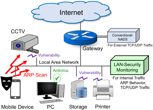
Figure 1: ARP scan calls made by LAN-internal malware are not visible to Conventional NADS, as these observe only incoming/outgoing (such as TCP/UDP) traffic. A LAN-security monitoring device attached to an internal LAN can observe this behaviour and protect connected devices, especially IoT.

Network Anomaly Detection Systems (NADS) are commonly placed, along with honeypots, at external gateways to catch intrusions (Baykara and Das, 2018). Honeypots aim to attract malicious traffic for purposes of detection, deflection and to study attempts to infiltrate the information system. Simple honeypots are easy to install and don’t require much resourcing, but have limited vision, and in addition, tend to generate excessive data with researchers having to resort to using open search analytics engines for evaluation (Almohannadi et al., 2018). To overcome this, honeypots are combined with NADS that are capable of detecting new attacks. However NADs themselves suffer from the problem of high false positive rates, which could result in “alert fatigue” (Ban et al., 2021).

Most NADs are unable to identify anomalies when only a few occur, resulting in rare anomalies easily slipping through. Thus, with most suspicious data packets captured by the NADS at the external gateway, only a few trickle through into the LAN. But these are now inside the LAN and could siphon privileged data if not detected early. Furthermore, as Figure 1 illustrates, in addition to these data packets entering the LAN, malware can enter via mobile devices connected to the LAN. Such malware would be categorised as insider attacks.

With insider attacks on the rise (IBM Security, 2020), predicting an attack within a LAN is becoming ever more crucial. The compromise of data of 10 million users, including identity documents, at an Australian Telecommunications company (Withers, 2022) was traced to an unsecured API and exposed access points. This and other similar events emphasise the need for better securing of internal LANs.

In the case of the Telecommunications breach (Withers, 2022) above, an internal LAN-security monitoring device may have identified the breach sooner, maybe preventing ex-filtration of so much data. Such monitoring would help protect devices connected to the LAN, especially IoT devices such as networked cameras, printers and storage. Our paper focuses on providing an additional layer of inner-LAN security that addresses seasonal and other patterns existing within LANs.

While internal LAN monitoring would add another layer of security, it comes with the downside that more false alarms are generated. Distinguishing critical security incidents from a barrage of false positives is not easy (Ban et al., 2021), making it important that minimal extra alerts are created by any additional layer of security. In Kandanarrchchi et al. (2022), a novel framework, Honeyboost, was introduced, where a honeypot coupled with a NADS, was deployed within a LAN. Honeyboost used Lookout (Kandanaarachchi and Hyndman, 2022), based on extreme value theory, to achieve low false positive rates. Using data from the LAN security monitoring project, the authors used data fusion techniques to integrate attributes from ARP, TCP and UDP protocols in two different ways, horizontal and vertical. Using only internal LAN data, the authors were able to identify anomalous nodes before they accessed the honeypot.

In this paper, we again use extreme value theory, which has the capability of handling fat tailed computer network traffic (Hernández-Campos et al., 2004). As shown in Kandanarrchchi et al. (2022), an anomaly detection method based on extreme value theory leads to significant reduction of false positives. In this paper, we model the network and forecast its behaviour using hierarchical forecasting techniques. Anomalies are identified by observing deviations from the forecast. To the best of our knowledge this is the first time such an approach has been used in computer network security.

We use ARP data from the LAN Security Monitoring Project (Sun et al., 2020; Ochiai, 2018) for our work. The address resolution protocol (ARP) is used by devices to locate the MAC address, given an IP address. However, ARP spoofing is easy, making the protocol a vulnerability in the LAN architecture (Cox et al., 2016). In this paper, we forecast the number of ARP calls made by each node using hierarchical time series methods. We use four forecasting techniques – machine learning and statistical-based – and three forecast reconciliation methods to adjust the original forecasts taking into account the total ARP calls. This allows us to come up with a final forecast for each node every hour. When a node does not stay true to its forecast behaviour, then it has possibly been subverted. We detect such anomalies using an extreme value theory-based method. We show that our method gives low false positives and can simulate complex seasonal patterns, one of the many challenges with detecting malware inside a LAN. These are patterns that change with the time of the day and the day of the week, and need to be taken into account when working with LAN data.

2 Background

Even when a network is protected at the Internet Gateway with a firewall or an intrusion detection system, malware can still be easily delivered to the local area network (LAN) through phishing e-mails or malware-infected mobile devices. Such malware infection will not be detected at the gateway, especially in the case of a targeted attack as the IP address used for the attack may not be blacklisted in the global threat sharing platform.

Figure 2: Places where intrusion detection systems can be deployed in LANs

LAN intrusion detection literature tends to focus on mechanisms that can be deployed at the external gateway. However, as shown in Figure 2, this is only a part of the bigger picture. The antivirus software installed on individual nodes performs a vital role in catching known viruses and malware. Unfortunately, new malware keeps constantly being developed and can easily escape the notice of antivirus software.

Snort architecture (Roesch et al., 1999) has been proposed to detect intrusions within computer networks. Snort architecture captures network traffic and gives an alert when any suspicious or malicious activities are detected. However, most snort-based systems (Garg and Maheshwari, 2016; Khamphakdee et al., 2014; Li and Liu, 2010) capture the communication traffic at the Internet gateway expecting the intruder within a LAN will attempt malicious communication with an external network entity. For example, scanning traffic towards the Internet could detect a DoS attack on an Internet server. Similarly, communication with a command–and–control (C&C) server could be detected with this architecture. Snort architecture originally used statistical-based or knowledge-based methods, but more recently, machine learning has also been deployed (Khraisat et al., 2019).

However, this approach is still not robust enough, especially in today’s cyberspace where the C&C server may not be blacklisted in the global database, and the payload of the communication between the C&C server could be encrypted with HTTPS. Today’s malware is targeted attack malware especially designed for specific organisations and will communicate with a C&C server which has not been discovered by security vendors. Such malware can make further expansions within a secured LAN without being noticed by Snort. The attacker can then steal the private information of the organisation and its customers, and hold the organisation to ransom, as has happened in many cases.

Furthermore, insider attacks and other threats described above can evade both of these mechanisms. As such, a LAN monitoring system taking into account only the behaviour inside the LAN adds a vital missing component to overall LAN security. We focus on such a LAN monitoring system in this work.

Given that we cannot rely on signatures such as IP addresses, a more promising venue would be behaviour-based detection or forecasting. We especially target the capture of internal expansion or internal spy activities that try to make further intrusions or retrieve information via direct communication between the hosts inside the local area networks. Given that such internal behaviour cannot be captured at the Internet gateway, a monitoring device is deployed inside a LAN as shown in Figure 1 and described in Section 4.1.

Many attacks on LANs have been studied (Kiravuo et al., 2013), with the security of LAN often discussed in terms of the vulnerabilities of address resolution protocols, such as ARP-spoofing (Whalen, 2001; Balogh et al., 2018) and ARP-poisoning (Nam et al., 2010). While there might be attacks on the LAN mechanism itself, here we wish to detect malware that uses LAN as a medium for expansion and further intrusion. Our approach is to monitor and use ARP behaviour broadcast over the entire LAN, to predict the behaviour of networked-malware. Such malware targets vulnerable TCP/UDP ports with the behaviour of ARP appearing as the side-channel effect of the behaviour of these ports.

OpenFlow (McKeown et al., 2008) has been proposed as an alternative form of local area network to control individual flows in the network. Since they can control all traffic inside the LAN, OpenFlow-based systems for LAN security have been proposed (Juba et al., 2013; Karakate et al., 2021), but OpenFlow is not yet very common in LAN environments.

Honeypot-based system for LANs have been proposed (Li et al., 2011) with large-scale data processing platforms for multiple LANs (Chirupphapa et al., 2022). Here, we take a honeypot-like monitoring approach.

In recent years, ARP has been used to detect suspicious behaviour of hosts in LANs. Zhang et al. (2020) proposed a detection method based on XGBoost. However, false positives were still a concern. In this paper, we forecast the ‘normal’ behaviour of the entire network by using hierarchical forecasting methods and find anomalous nodes that deviate from the normal by using an extreme value theory based method that gives low false positives.

Regression methods and, in particular, forecasting in various forms are powerful analytical methods used to predict network attacks. Attack graphs are popular tools in risk management, used for predicting attacks on networks (GhasemiGol et al., 2016). Attack graphs extract rules and utilise information from other nodes to determine the probability of attacks from different services. While determining rules is a common technique to identify attacks on systems, more recent work attempts the use of appropriate time series forecasting methods that are suitable for detecting the security vulnerabilities of IT systems, i.e., those capable of dealing with non-stationarity, seasonality, and intermittency. Yasasin et al. (2020) used exponential smoothing methods, Croston, Arima, and neural networks to forecast the number of post-release security vulnerabilities in browsers, operating systems and office solutions. They suggest the use of different forecasting methods, based on the system and problem. However, Yasasin et al. (2020) use conventional methods for forecasting and do not leverage the more advanced methods available, such as, using explanatory variables, hierarchical forecasting, or tree-based models. Vulnerabilities have been detected in a similar manner by using time series methods (Roumani et al., 2015).

Anomaly detection is a popular method for detecting cyber attacks and intrusion detection. For instance, Landauer et al. (2018) propose a clustering framework that considers the dynamic nature of log file data for anomaly detection. While anomaly detection is typically used for detecting attacks, it is possible to predict attacks by using forecasting methods. Evangelou and Adams (2020) use a set of features and several regression methods to forecast the number of traffic events for an individual device. They set a limit for normal forecasts and identify the forecasts that lie outside the limit forecasts as anomalies. They compare their model with benchmarking methods such as Pruned Exact Linear Time as and empirically show that the quantile regression model is effective. They do not explore the efficacy of machine learning methods or classical features of time series such as seasonality. We will explore these features in this study in addition to using the hierarchical information in the network.

2.1 Strengths of our approach

Each component in our methodology has a unique purpose that contributes to synergy of the entire approach.

1. Extraction of latent and cross-sectional information by hierarchical forecasting: Time series forecasting methods can model complex trend and seasonality patterns in data. If the network traffic fluctuates due to time of day or the day of the week, the forecast can account for this behaviour. While historical observations can be useful for predicting the future behaviour, we can use more advanced techniques such as hierarchical forecasting to extract more information from other nodes that may be useful for predicting the behaviour of a particular node. The benefit of this technique is the generation of more accurate forecasts for all nodes.

2. Using residuals to account for heterogeneous behaviour: By considering residuals we can focus on the deviations from expected behaviour. This is different from considering just the observed values $y_{i,t}$, of a node $i$ at time $t$, as these observed values can be time dependent. For example, a node used by a particular user can result in a high volume of network traffic, corresponding to large $y_{i,t}$ at certain times every day. While this kind of behaviour would be expected from this particular node, the same behaviour might be anomalous for another node. Hence, if we detect anomalies from just the observed values $y_{i,t}$, then we’re assuming homogeneous, non-time dependent behaviour from all the nodes. The use of residuals, effectively, lets us construct a personalised model for each node.

3. Low false positives using EVT for anomaly detection: As we will explain later (see Section 3.4), Extreme Value Theory (EVT) based methods produce low false positives due to their ability to handle fat tails. Furthermore, we use a data-driven anomaly detection method that derives parameters from the data.

3 Methodology

This section details the methodologies we use for the research in this paper.

3.1 Defining anomalous behaviour

Hawkins (1980) states the intuitive definition of an outlier would be ‘an observation which deviates so much from other observations as to arouse suspicions that it was generated by a different mechanism’. An inspection of a sample containing outliers would show up such characteristics as large gaps between ‘outlying’ and ‘inlying’ observations and the deviation between the outliers and the group of inliers, as measured on some suitably standardized scale.

Such large gaps in the data can be observed in a setting where observations are independently and identically distributed (iid). However, when detecting anomalies in multiple time series, this is not always the case as we need to account for dynamic behaviour. Consequently, it is necessary to translate the intuitive definition given above into more concrete mathematical terms. Let $\{y_{t}\}_{t=1}^{N}$ denote a univariate time series. In a time series setting, we define an anomaly as a point with low conditional probability given its past history. We denote the conditional probability of $y_{t}$ given its past values as

$$p_{t|t-1}=\mathcal{P}\left(y_{t}|y_{t-1},\ldots,y_{1}\right)\,.$$ (1)

If $y_{t}$ is anomalous, then the likelihood of observing $y_{t}$ is low, i.e., it has low conditional probability. But how do we compute this conditional probability? We start by modelling the time series using statistical and machine learning methods.

3.2 Hierarchical time series

Hierarchical time series refers to a collection of time series that are nested in a meaningful structure. We can classify hierarchical time series into two categories: i) cross-section hierarchies where (geographical) location is the feature of aggregation and disaggregation, and ii) temporal hierarchies where time is the feature of aggregation and disaggregation. Cross-temporal is another category that is essentially a combination of both cross-sectional and temporal hierarchies with both location and time being features of interest for aggregating and disaggregating the time series. Time series naturally have a hierarchical format as they can be aggregated and disaggregated by different features. For example, in a cybersecurity setting, we can consider the signal for an individual computer as one node, and we can then aggregate these signals to find out the total signals in a computer network.

Hierarchical forecasting (HF) is necessary because we often need to extract different information from the network that may be useful for various decisions. For example, total number of signals is needed to plan for infrastructure requirements, while individual signals are needed to understand the behaviour of an individual node. Another important motivation to use HF is their usefulness in improving forecasting accuracy because they can extract and use information from different levels and nodes to improve forecasting accuracy that may otherwise not be apparent in any one single level.

Different techniques can be used for HF including bottom-up (BU), top-down (TD), and minimising trace (MinT). We will describe these methods in section 3.2.1. These techniques are used to ensure forecasts are coherent across different levels, i.e., forecasts add up properly in the hierarchy. Forecasts for each node can be generated using any forecasting model that may be appropriate for the time series. However, if series are foretasted individually they may not be consistent from one level to another, i.e., the sum of the base forecasts may not be equal to the forecast of the sum. Therefore, hierarchical forecasting techniques are employed after forecasting the series to ensure coherency in the hierarchy (Hyndman and Athanasopoulos, 2021).

3.2.1 General framework

We first introduce some notation to describe hierarchical forecasting methods. We consider $m$ time series, each belonging to a unique node. Let $\{y_{i,t}\}_{t=1}^{N}$ denote the time series of the $i^{th}$ node with $N$ observations, $m$ be the total number of series in the hierarchy with $m_{i}$ being the total number of the series for level $i$, $k$ the total number of the levels in the hierarchy, $\bm{Y}_{i,t}$ the vector of all observations at level $i$, $\hat{\bm{Y}}_{i,t}(h)$ the $h$ step ahead forecasts at level $i$, $\bm{Y}_{t}$ a column vector including all observations, $\hat{\bm{Y}}_{n}(h)$ the $h$-step-ahead independent base forecast of all series based on $n$ observations, and $\tilde{\bm{Y}}_{n}(h)$ the final reconciled forecasts of all series. A hierarchical time series can be shown using the unified equation $\bm{Y}_{t}=\bm{S}\bm{Y}_{k,t}$, where $\bm{S}$ is a summing matrix of order $m\times m_{k}$ that aggregates the series at the bottom level $k$. For example, Figure 3 gives the two-level hierarchical time series. In this hierarchy, $Y_{t}$ is the total value of nodes at time $t$, $Y_{A,t}$ is the value of node $A$ at time $t$, and $Y_{B,t}$ is the value of node $B$ at time $t$.

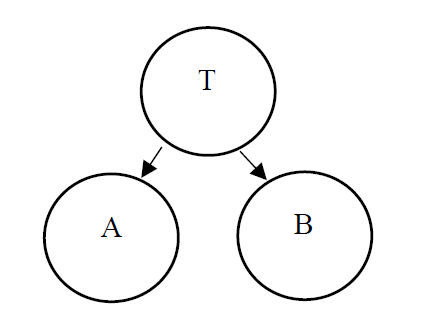
Figure 3: A two-level hierarchy. Nodes A and B are at the bottom and T represents the total at the top.

To show this hierarchy we can use the matrix below:

$$\left[\begin{array}[]{c}Y_{t}\\ Y_{A,t}\\ Y_{B,t}\\ \end{array}\right]=\left[\begin{array}[]{@{}*{2}{c}@{}}1&1\\ 1&0\\ 0&1\\ \end{array}\right]\times\left[\begin{array}[]{c}Y_{A,t}\\ Y_{B,t}\\ \end{array}\right]$$

It is common to forecast the series within a hierarchy individually (these are called base forecasts) and then map them in the hierarchy with the aggregation structure to obtain the reconciled forecasts. In such a setting, we can depict hierarchical time series with $\tilde{\bm{Y}}_{n}(h)=\bm{S}\bm{G}\hat{\bm{Y}}_{n}(h)$, where $\hat{\bm{Y}}_{n}(h)$ is the base forecasts of series, $\tilde{\bm{Y}}_{n}(h)$ is the reconciled forecasts, and $\bm{G}$ is a matrix of order $m\times m_{k}$ that maps all the forecasts to the bottom level which can then be aggregated with the summing matrix $S$ to higher levels. The elements of matrix $G$ can be estimated with different hierarchical forecasting techniques as follows:

• BU: In this method, we simply forecast all series individually at the lowest level of the hierarchy and sum them up to obtain the forecast for their parent time series at higher levels. Therefore, $\bm{G}$ takes the forecasts at the bottom level and combines them to obtain the forecasts at higher levels for their parent nodes.

• TD: In this method, we generate a forecast only at the top level for the most-aggregated node. Then, forecasts can be disaggregated to their children nodes to obtain their individual forecasts. Several methods have been proposed to break down the forecast in the TD method. We use the simple form of historical proportions, i.e., the portion of forecasts for each child node will be the same as the average of its historical proportions from its parent node. This is a simple method and has been shown to work well in various settings. Thus, the proportion of node $j$, $p_{j}$, is computed as follows: $p_{j}=\frac{\sum_{t=1}^{n}Y_{j,t}}{\sum_{t=1}^{n}Y_{t}}$. We can then construct the vector $\bm{g}=[p_{1},p_{2},p_{3},\dots,p_{m_{k}}]$ and matrix $\bm{G}=[\bm{g}\mid\bm{0}_{m_{k}\times(m-1)}]^{\prime}$.

• MinT: The MinT method is more advanced than the TD and BU methods. Unlike TD and BU which generate forecasts for the very ends of a hierarchy, MinT produces individual base forecasts for all the series in the hierarchy and then reconciles them with a linear model. Let $\tilde{\bm{Y}}_{n}(h)=\bm{S}\bm{G}\hat{\bm{Y}_{n}}(h)$ denote the $h$ step ahead reconciled forecasts. The covariance matrix of the forecast errors is given by

  $$\bm{V}_{h}=\text{Var}[\bm{y}_{n+h}-\tilde{\bm{Y}}_{n}(h)]=\bm{S}\bm{G}\bm{W}_{h}\bm{G}^{\prime}\bm{S}^{\prime},$$

  where $\bm{W}_{h}$ is the variance-covariance matrix of the $h$-step-ahead base forecast errors, $\bm{S}^{\prime}$ is the transpose of matrix $S$, and $\bm{G}^{\prime}$ is the transpose of matrix $G$ (Wickramasuriya et al., 2019). In this case, $\bm{G}$ can be estimated via $\bm{G}=(\bm{S}^{\prime}\bm{W}^{\dagger}_{h}\bm{S})^{-1}\bm{S}^{\prime}\bm{W}_{h}^{\dagger},$ where $\bm{W}^{\dagger}_{h}$ is the generalized inverse of $\bm{W}_{h}$. Although not always easy, different techniques can be used to estimate $\bm{W}_{h}$. We use Shrinkage to estimate the matrix which is a commonly used technique shown to work well (Spiliotis et al., 2021; Wickramasuriya et al., 2019).

Hierarchical series have been shown to be useful in extracting data from nested series. Series at different levels of the hierarchy can reveal different information that may be useful for forecasting an individual node. Therefore, they can be used for extracting latent information from other nodes and levels that may not be apparent in one single node (Abolghasemi et al., 2022a, b). In this study, we build a two-level hierarchy, similar to 3, with 362 nodes at the bottom level indicating 362 Mac addresses, and one node at the top indicating the total ARP calls in the network.

3.3 Forecasting methods

We train four different forecasting methods, including simple and advanced statistical as well as machine learning models, to forecast the behaviour of every single node. We then leverage the hierarchical structure of the network and reconcile the forecasts for nodes using the above-mentioned hierarchical forecasting methods.

The first forecasting method we use is exponential smoothing. We use the so-called state-space exponential smoothing (ETS) framework for training the models and forecasting (Hyndman and Athanasopoulos, 2021). Exponential smoothing is a simple but powerful statistical model that has been successfully implemented in various forecasting tasks (Hyndman and Athanasopoulos, 2021). This method takes a weighted average of past observations with the most recent observations getting a larger weight, to estimate future values. Several variations of exponential smoothing have been proposed where different variations can be considered for errors, trends, and seasonality in data. ETS method considers the error, trend, and seasonality type for each series, trains different models, and chooses the best model by minimising Akaike Information Criteria (AIC). The forecasts are then generated based on the best model. This method is implemented using the ‘fable’ package in the open-source R programming language.

The second forecasting method is a time series linear regression model (TSLM). This is essentially a regression model that regresses the response variable (signals) as a linear function of the explanatory variables. We use the trend and the last six observations of the series as the explanatory variable. We also use a logarithm of signals as the response variable, enabling the log-linear model to better estimate the non-linear behaviour of the signal time series (Hyndman and Athanasopoulos, 2021). Note that we add a small number to the signals to avoid any issues in taking the logarithm of signals when they take the value of zero. This method is implemented using the ‘fable’ R package.

The third model that we use is the Zero-Inflated Negative Binomial model. This model essentially gives considerable attention to the many zeros present in the signal time series data, while at the same time, the Negative Binomial takes into account the large spikes that may arise after these zeros. We use the last six observations of signals as the regressors of the model and implement the model using ‘pscl’ R package.

The last and final forecasting model implemented is Light Gradient Boosting Model (LightGBM), a powerful Machine Learning (ML) model, which was the top-performing model in several forecasting competitions, achieving great results in numerous applications (Abolghasemi et al., 2022b, a). We optimise the hyperparameters of the LightGBM model with Grid Search. We opt to optimise the most important hyperparameters including ‘Number of Leaves’ ranging from 80 to 120, ‘minimum number of observations in leaf’ ranging from 100 to 200, ‘learning rate’ ranging from 0.05 to 0.5, and ‘maximum depth’ ranging from 8 to 12, to avoid the computational burden of running many experiments. We optimise the hyperparameters once and share them across the horizon. This model is implemented using the ‘lightgbm‘ R package.

3.3.1 Residuals and anomalies

The forecasting methods discussed in Sections 3.2 and 3.3 model each time series and give a reconciled forecast $\hat{y}_{i,t}$ taking into account the aggregated time series. Thus, $\hat{y}_{i,t}$ encompasses the expected behaviour of node $i$ at time $t$. The time series forecasting models ensure the residuals

$$e_{i,t}=y_{i,t}-\hat{y}_{i,t}\,,$$ (2)

are normally distributed, i.e., $e_{i,t}\sim\mathcal{N}(0,\sigma_{i}^{2})$ where $\sigma_{i}$ denotes the standard deviation of residuals for node $i$. Therefore, the probability of large absolute residuals is low. However, large absolute residuals occur when the forecast is quite different from the actual. If the forecasting models are good, when $y_{i,t}$ behave as expected the forecast $\hat{y}_{i,t}$ is a good approximation of $y_{i,t}$, giving rise to small residuals $e_{i,t}$. That is, if we assume the forecasting models capture the time dependency of $\{y_{i,t}\}_{t=1}^{N}$ the conditional probability $p_{i,t|t-1}=\mathcal{P}\left(y_{i,t}|y_{i,t-1},\ldots,y_{i,1}\right)$ satisfies

$$p_{i,t|t-1}\geq\epsilon\iff|e_{i,t}|\leq c\left(\epsilon\right)\,,$$ (3)

where $\epsilon$ is small. This reiterates that the expected behaviour of $y_{i,t}$ has a high conditional probability, resulting in small residuals. Anomalies are different and certainly not expected. Thus, anomalies have low conditional probabilities and anomalous $y_{i,t}$ exhibit large residuals, i.e.,

$$p_{i,t|t-1}\leq\epsilon\iff|e_{i,t}|\geq c\left(\epsilon\right)\,.$$ (4)

We identify anomalous $y_{i,t}$ by focusing on the residual space. Before identifying anomalies we briefly discuss Extreme Value Theory.

3.4 Anomaly detection using Extreme Value Theory (EVT)

Computer network traffic exhibit heavy-tails (Ramaswami et al., 2014; Hernández-Campos et al., 2004). Hernández-Campos et al. (2004) show the time taken by IP flows have very large values than can be expected by a typical exponential distribution; they explain this using heavy-tailed distributions. The heavy-tailed property in computer traffic has multiple implications. If not taken care of at a fundamental level, it can result in an ‘alarm factory’ giving rise to ‘security fatigue’ (Furnell and Thomson, 2009), a big problem when it comes to security event management. Unfortunately, most alerts are false alarms that cause much wastage of operator time and energy, while the real attacks get low priority or are unattended.

High false alarm rates can be mitigated using techniques from Extreme Value Theory (EVT), which can incorporate different types of tails. We briefly explore the 3 types of tail behaviour given by Gumbell, Fréchet and Weibull distributions. Figure 4 shows these families of distributions. The focus is on large values which correspond to the right tail. Weibull distributions have truncated right tails, i.e., the maximum is bounded. Gumbel distributions have exponentially decaying tails. Fréchet distributions have heavy tails that are not exponentially bounded.

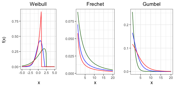
Figure 4: Different tail behaviour. Weibull distribution has a truncated tail. Gumbell has an exponentially decaying tail and Frechet has a fatter tail.

The cumulative distribution functions $\mathcal{P}\left(X\leq x\right)$ of these 3 distributions are given by

$$\text{Gumbel:}\quad G(x) =\exp\left(-\exp\left[-\left(\frac{x-b}{a}\right)\right]\right)\,,\quad-\infty<x<\infty\,$$ (5)

$$\text{Fr\'{e}chet:}\quad G(x) =\begin{cases}0\,,&x\leq b\\ \exp\left(-\left(\frac{x-b}{a}\right)^{-\alpha}\right)\,,&x>b\\ \end{cases}$$ (6)

$$\text{Weibull:}\quad G(x) =\begin{cases}\exp\left(-\left(-\left[\frac{x-b}{a}\right]\right)^{\alpha}\right)\,,&x<b\\ 1\,,&x\geq b\\ \end{cases}$$ (7)

where $a,b$ and $\alpha$ are parameters and $a,\alpha>0$. When fitting models to real-world applications, these parameters are derived from the data.

Consider $n$ independent and identically distributed random variables $X_{1},\ldots,X_{n}$ and let $M_{n}=\max\left(X_{1},\ldots,X_{n}\right)$. Then the Fisher-Tippet-Gnedenko Theorem (Coles et al., 2001) states that a scaled version of $M_{n}$ has certain limit distributions.

Theorem 1

(Fisher-Tippet-Gnedenko) If there exists sequences $\{a_{n}\}$ and $\{b_{n}\}$ such that

$$\mathcal{P}\left(\frac{(M_{n}-b_{n})}{a_{n}}\leq x\right)\to G(x),\quad\text{as}\quad n\to\infty,$$

where $G$ is a non-degenerate distribution function, then G belongs to either the Gumbel, the Fréchet or the Weibull family.

Simply put, the Fisher-Tippet-Gnedenko Theorem states that the tails of any decent distribution can be modelled by Gumbel, Fréchet or Weibull families. This is the equivalent of the Central Limit Theorem (CLT) to sample maxima. CLT finds a limiting distribution to the sample mean whereas the Fisher-Tippet-Gnedenko Theorem finds 3 families of limiting distributions to model the sample maximum. These 3 distribution families – Gumbel, Fréchet and Weibull – cover all possible tail behaviour for non-degenerate distribution functions.

The Generalized Extreme Value (GEV) distribution given by

$$G(x)=\exp\left(-\left[1+\xi\left(\frac{x-\mu}{\sigma}\right)\right]^{-1/\xi}\right)\,,$$ (8)

with the domain $\{x:1+\xi(x-\mu)/\sigma>0\}$ encompasses all three distributions with the parameter $\xi$. When $\xi=0$ we obtain the Gumbel distribution, $\xi>0$ gives Fréchet and $\xi<0$ gives Weibull distributions.

A criticism of GEV related approaches when modelling real-world applications is data wastage. As GEVs are used on sample maxima, a lot of data ends up not being used. This is detrimental because some samples can have values larger than the maximum value of other samples. Thus, taking only the sample maxima is sub-optimal to say the least. The Peak Over Threshold (POT) approach that uses the Generalised Pareto Distribution (GPD) remedies this issue. While GEVs are used to model sample maxima, GPDs are used to model large values, typically greater than a given threshold $u$. GPDs and GEVs are linked by the following theorem.

Theorem 2 (Pickands)

Let $X_{1},\,X_{2},\ldots,\,X_{n}$ be a sequence of independent random variables with a common distribution function $F$, and let

$$M_{n}=\max\left(X_{1},\ldots,X_{n}\right)\,.$$

Suppose $F$ satisfies Theorem 1 so that for large $n$

$$\mathcal{P}\{M_{n}\leq z\}\approx G(z)\,,$$

where

$$G(z)=\exp\left\{-\left[1+\xi\left(\frac{z-\mu}{\sigma}\right)\right]^{-1/\xi}\right\}\,,$$

for some $\mu,\xi\in\mathbb{R}$ and $\sigma>0$. Then for large enough $u$, the distribution function of $(X-u)$ conditional on $X>u$, is approximately

$$H(y)=1-\left(1+\frac{\xi y}{\sigma_{u}}\right)^{-1/\xi}\,,$$ (9)

where the domain of $H$ is $\{y:y>0\,\,\text{and}\,\,(1+\xi y/\sigma_{u})>0\}$  , where $\sigma_{u}=\sigma+\xi(u-\mu)$.

input    :   A collection of ARP time series $\{y_{i,t}\}_{t=1}^{N}$, where $i$ denotes the node,

initial training window length $L_{\text{train}_{1}}$,

test window length $L_{\text{test}}$

frequency of forecasts (e.g. hourly) and

preferred time series forecasting method from

{ETS, TSLM, Zero-inflated, LightGBM},

preferred forecast reconciliation method from

{BU, TD, MinT}

output :   The anomalous nodes and the respective timestamps

1 Let $t_{0}$ and $t_{\max}$ denote the initial and final times.

2 Let $j=1$ and $t_{\text{train}_{j}}=t_{0}+L_{\text{train}_{1}}$.

3 Let $t_{\text{test}_{j}}=t_{\text{train}_{j}}+L_{\text{test}}$.

4 while $t_{\text{test}}\leq t_{\max}$ do

5       $Y_{\text{train}}=\{y_{i,t}\}$ for $t<t_{\text{train}_{j}}$ for all $i$ in collection.

6       $Y_{\text{test}}=\{y_{i,t}\}$ for $t_{\text{train}_{j}}\leq t<t_{\text{test}_{j}}$ for all $i$ in collection.

7       Fit the preferred time series forecasting model to the training set $Y_{\text{train}}$ and obtain initial forecasts.

8       Consider a hierarchy similar to that in Figure 3 and reconcile the initial forecasts using the preferred reconciliation method as explained in Section 3.2. Let the reconciled individual forecasts for each node and each time stamp be denoted by $\hat{y}_{i,t}$.

9       Let $e_{i,t}=y_{i,t}-\hat{y}_{i,t}$ denote the residuals.

10       Use lookout on $\{e_{i,t}\}$ to find anomalies.

11       $j:=j+1$

12       Advance the training set; let $t_{\text{train}_{j}}=t_{\text{train}_{j}}+L_{\text{test}}$

13       Advance the test set; let $t_{\text{test}_{j}}=t_{\text{train}_{j}}+L_{\text{test}}$.

14 end while

Algorithm 1 Detecting anomalous nodes inside LANs.

The GPD parameters can be derived from the GEV parameters; the shape parameter $\xi$ is the same in both formulations. The POT approach considers $X$ greater than $u$, i.e., $\{X|X>u\}$ and models them using a GPD.

Using EVT to detect anomalies has gained popularity in recent years (L, 2018; Talagala et al., 2021). One of the main reasons being EVT methods result in low false positives because they can handle heavy tails. This is especially applicable to computer traffic data. We use an anomaly detection method named lookout (Kandanaarachchi and Hyndman, 2022) that uses the POT approach with GPDs to identify anomalies. Lookout computes the kernel density estimates of the data and finds anomalies in low density regions by modelling the $-\log(\text{density}(x))$ as a GPD. The function $-\log(\text{density}(x))$ maps low density points to high values so that the GPD models these large values, effectively focusing on low density regions. Points in suspiciously low density regions are flagged as anomalies. We summarize this method in Algorithm 1.

4 The experimental setup and results

Figure 5: Types of intrusion detection datasets

4.1 Dataset

This research uses data from the LAN-Security monitoring project (Sun et al., 2020; Ochiai, 2018), a research collaboration led by Japan and involving 12 ASEAN and SAARC countries. Deployed in late 2018, the research project aimed to improve cyber-readiness and cyber-resilience among the partners.

Figure 6: The LAN monitoring device. This is connected to a LAN as a host – not to a mirror port of the switch. This easy-installation design for monitoring suspicious activities is important especially in ASEAN and SAARC countries, where security incidents are very common because of the lack of detection/protection infrastructure.

The dataset used in this paper was generated by deploying a monitoring device (see Figure 6 ) on a local-area network (LAN) of a laboratory network from January to December 2019 . This device joined the network with a given IP address and monitored both the traffic broadcast over the entire network as well as the packets directed at the monitoring device, by using the Linux tcpdump command. The captured broadcast traffic includes address resolution protocol (ARP) requests. An ARP request has source and target IP addresses for looking up the MAC address for forwarding IP packets. Each ARP request is identified with its sender’s MAC address because the source IP address may change based on the assigning policy of the DHCP server of the network.

Before malware in a host on the network discovers available open TCP/UDP ports for further intrusion into remote operating systems or retrieves information from file servers, it tries to find available hosts in the network, by sending IP packets one by one expecting responses from them. During this activity, many ARP requests with changing target IP fields are observed because the sender wishes to know the target MAC addresses. The target device responds to the ARP request and receives IP packets from the malware. If the device is vulnerable to the IP packets, it will be compromised.

When such an attack is carried out on any of the hosts in the network, the monitoring device also receives TCP/UDP-layer-contained IP packets from the sender along with the observed sequences of broadcast ARP requests. There is no legitimate reason for a host to send a TCP/UDP packet to the monitoring device. Therefore, we consider all nodes that access the monitoring device as anomalies, and treat the monitoring device as a source for ground truth labels. Here, we investigate whether we can identify the anomalous nodes using only ARP behaviour, using the TCP/UDP data of the monitoring device to validate our results.

4.2 Ground-truth labels and the dataset used here

In the vast world of real data ($X$) available for research, there exist few with ground-truth labels ($y$). Datasets containing simulated behaviour could have ground-truth labels $y$ but are often collected during small time intervals or are simulated in a very specific way. Therefore, these datasets do not really replicate real data $X$. Thus, real-world data comes in different forms (see Figure 5). While most research in the application of machine learning to security uses data with ground-truth labels ($y$), the focus of this study is a real dataset ($X$) with no inherent ground-truth labels, which makes this research unique.

Cyber security research has profited enormously from the construction and availability of many datasets. Older cyber security datasets such as KDDCup’99 have been studied in depth, and newer datasets, such as the UNSW-NB15 Dataset (Moustafa and Slay, 2015), introduced to mitigate some of the limitations of previous datasets and to account for newer attacks. Most datasets, such as UNSW-NB15 and CIC-MalMem-2022 (Carrier et al., 2022), include data from orchestrated or simulated attacks, in summary ‘artificial’ user activity (Hignam et al., 2021). Given the attacks are simulated, it is possible to label these datasets, as has been done. The rapid growth of cybercrime and new attacks, however, means that the sort of attacks that can be simulated would form only a small subset of existing (and future) attacks. Indeed, the BETH dataset (Hignam et al., 2021) continues to be expanded as (new) attack vectors are added.

Furthermore, when data from a relatively long period of time is included, it is hard to be certain that everything other than the simulated attacks are actually non-malicious. That is, the possibility exists that some of the data labelled as normal is actually malicious.

To address these concerns, we adopted a different approach to dataset generation. Our dataset does not have orchestrated or simulated attacks. Instead, our data was captured from an internal-LAN setting from January to December 2019. Thus, the dataset used in this research, is a collection of observed LAN traffic without any simulations. Therefore, in its original form it is unlabelled. Of course, to evaluate our proposed scheme, we need to assign some (virtual) labels as this allows us more flexibility in the evaluation of the anomalies. The intrusions or anomalies were determined using a LAN monitoring device, which we described in the previous section. The data that is used in this paper can be found at https://github.com/sevvandi/supplementary_material/tree/master/forecasting_and_anomaly_detection.

4.3 Data preprocessing and time windows

The original data, captured from January to December 2019, is of the form $\left(t_{i},\text{node}_{t_{i}}\right)$. This dataset has 10,309,621 such entries from 362 nodes all relating to ARP calls. For a given time $t_{i}$ there can be more than one host, $\text{node}_{t_{i}}$, making ARP calls in the network. We transform the data into a time series format by considering hourly aggregates and rearranging it by node id. Then for each node $i$ we have a time series $\{y_{i,t}\}_{t=1}^{N}$. We note that for certain time periods $y_{i,t}$ can be zero. As the dataset is from a laboratory computer network, there will be a high volume over certain periods, while the volume will be low during university holidays.

We consider an initial time period of two months to fit the time series forecasting models; we denote this period by $[t_{0},t_{\text{train}_{1}}]$. Using these models we forecast hourly ARP calls for each node for the next week. This is the first test period, spanning $[t_{\text{train}_{1}},t_{\text{test}_{1}}]$, where $t_{\text{test}_{1}}$ denotes the end of the first test week. For each week we have $24\times 7$ forecasts for each node. We use a rolling/expanding window model in which the $i^{\text{th}}$ training period spans $[t_{0},t_{\text{train}_{i}}]$ and the $i^{\text{th}}$ test period spans the week $[t_{\text{train}_{i}},t_{\text{test}_{i}}]$. This sets up results in approximately 42 weeks of rolling hourly forecasts for each node.

4.4 Evaluation

Each user in a computer network does different things, which manifests differently in the ARP space as evidenced by Figure 7. Indeed, the ARP call patterns are quite diverse. We note that users can connect to the LAN via laptops, desktops, tablets, mobile phones or other devices. Nodes N003 and N004, for example, are active in the network from Day 1 to Day 70. In the university the data was collected, day 70 roughly corresponds to the time of graduation, which explains this behaviour. Furthermore, N005 consistently makes a very large number of ARP calls compared to the other nodes. Upon inspection we find that N005 corresponds to the network router.

In situations where there are diverse behaviour patterns, our definition of an anomaly becomes very useful because an anomaly is defined as a point with low conditional probability. Conditioned on its previous behaviour, the probability of a node’s behaviour at time $t$ is computed using the residuals. Thus, a node is declared anomalous if its behaviour is substantially different with respect to its previous behaviour. This formalisation better suits heterogeneous behaviour – where each node behaves differently from others – and anomalies are declared when a node behaves considerably different from its regular behaviour.

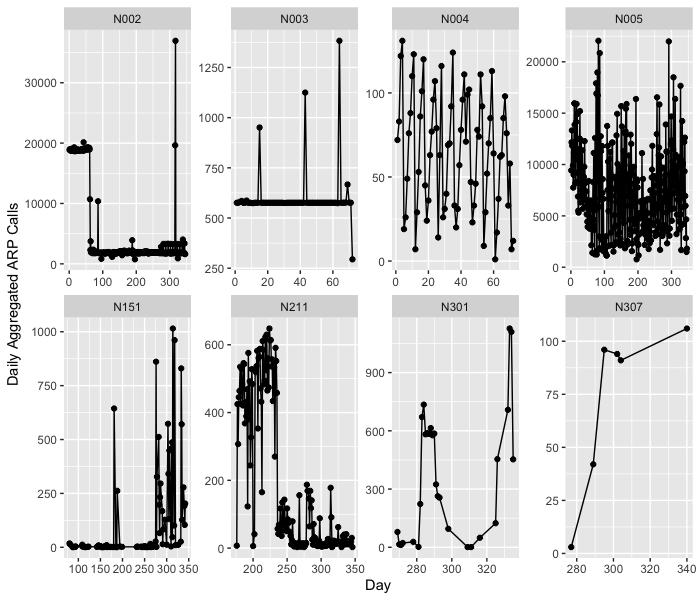
Figure 7: ARP calls of 8 representative nodes (out of over 300 nodes) in the LAN data collected as noted in Section 4.1

As discussed before, we train different forecasting models for each node and then reconcile the forecasts with various hierarchical forecasting methods. This results in different forecast accuracy for the hierarchy and the investigated methods. Although we report the forecasts’ accuracy results, we note that improving the accuracy of the forecasts is not the goal here. Instead, forecast accuracy and residuals will be used as a proxy to detect abnormal behaviour in nodes. We report the accuracy of methods here to merely depict the normal behaviour of forecasting models in predicting the pattern of signals. Table 1 shows the summary of the forecast accuracy of each method in terms of mean absolute error (MAE) across all nodes, on average. As we can see, the average forecast accuracy is lower (higher MAE) for anomalous nodes than for non-anomalous nodes (lower MAE). The lower accuracy for non-anomalous nodes is caused by highly unpredictable behaviour of these nodes that is triggered by larger ARP calls. The deviation in forecast accuracy is representative of abnormal behaviour in the series which will be used to detect the anomalous behaviour of the nodes. We observe a higher forecast accuracy for LightGBM and ZeroInflated models and lower accuracy for ETS and TSLM models for anomalous and non-anomalous nodes, respectively. In terms of the different hierarchical forecasting techniques, we observe different behaviour across the existing methods. However, BU and MinT often out-performs the other methods for both anomalous and non-anomalous nodes. So, we use the various generated forecasts from BU and MinT methods for further analysis in this study. However, the results from any other method can be used.

Table 1: Forecast accuracy of methods in mean absolute error (MAE) reported for 14 anomalous and 348 non-anomalous nodes. Low accuracy corresponds to high MAE and vice versa.

Method	Anomalous nodes	Non-Anomalous nodes	All
ETS-BU	76.13	2.16	5.44
ETS-TD	76.10	3.40	5.72
ETS-MinT	77.70	2.21	5.83
TSLM-BU	32.21	8.49	5.29
TSLM-TD	32.31	8.59	5.39
TSLM-MinT	30.20	8.09	5.29
LightGBM-BU	31.37	3.54	4.57
LightGBM-TD	31.22	4.09	5.14
LightGBM-MinT	31.53	5.53	3.84
ZeroInflated-BU	17.97	1.14	1.80
ZeroInflated-TD	27.52	2.91	3.86
ZeroInflated-MinT	18.26	1.44	2.09

After fitting the hierarchical time series models and forecasting hourly ARP calls by node for each test week, we compute the residuals. Figure 9 shows the residuals of 4 nodes for the ETS model by hour. While some nodes have large residuals, some have smaller residuals. The data exhibits complex patterns and a simple threshold method (absolute residual $>$ threshold $\Rightarrow$ anomaly) would not suffice even though Table 1 shows a distinction between anomalies and non-anomalies. The underlying reason is that Table 1 lists averages and hourly ARP calls have a more complex behaviour. Figure 9 shows all the residuals by time, with the weeks shown in dotted lines. The hourly residuals for each week are fed into the lookout anomaly detection algorithm. Lookout identifies the anomalous ARP calls for each week. As a comparison, we employ an autoencoder on the same input data (aggregated hourly ARP values by node) and report results.

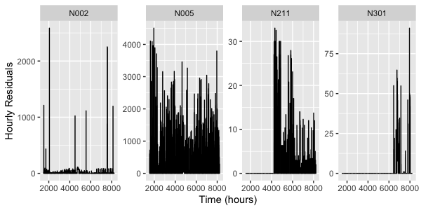
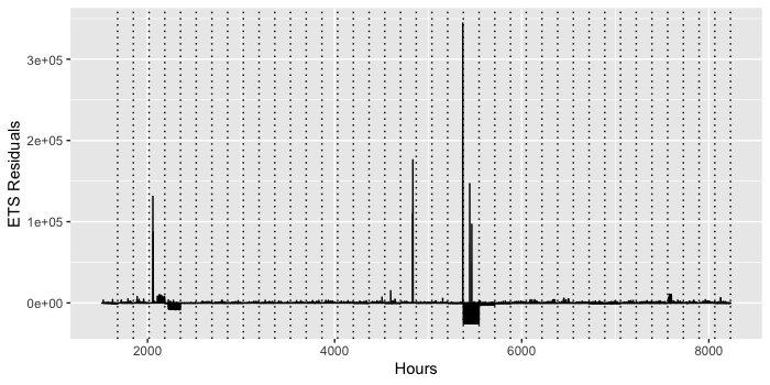
Figure 8: ETS hourly residuals for 4 nodes in the LAN.

Figure 9: ETS Residuals by hour with weeks shown in dotted lines.

Table 2 gives the mean and standard deviation in brackets for precision, recall, F-measure and the number of false positives per window for all methods. We see that the hierarchical methods BU and MinT give almost identical results. Figures 11 and 11 show the boxplots with the data points. From both Table 2 and Figures 11 and 11 we see that LightGBM has the highest F-measure followed by TSLM and Zero-inflated models. The lowest F-measure is achieved by the autoencoder. Similarly, LightGBM, ETS and Zero-inflated models have very low false positives per each time window. TSLM has a slightly higher number of false positives, but the autoencoder has a much larger number of false positives per window. LightGBM has the highest precision of the 5 models, followed by the Zero-inflated model. The autoencoder achieves higher recall values compared to ETS and TSLM. A higher recall is expected when many points are identified as belonging to the positive class. Even though ETS and TSLM have lower recall values compared to the autoencoder, from Figure 11 we see that they are still comparable. LightGBM has the lowest recall values of the 5 methods. Overall, LightGBM performs better than the other methods, while the autoencoder performs the poorest. In a way this is to be expected because we take the diversity of nodes into account by using hierarchical forecasting methods and have used anomaly detection methods based on extreme value theory that ensures low false positives.

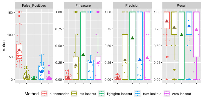
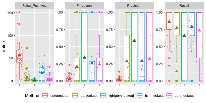
Figure 10: Comparison of results using an autoencoder, ETS-lookout, LightGBM-lookout, TSLM-lookout and Zeroinflated-lookout using BU as hierarchical forecasting method.

Figure 11: Comparison of methods using MinT for hierarchical forecasting. Autoencoder used as a comparison method.

Table 2: Comparison of results

Hierarchical method	Forecasting and AD method	False positives	Precision	Recall	F-measure
	ETS-lookout	6.073 (7.481)	0.286 (0.428)	0.769 (0.382)	0.208 (0.362)
BU	TSLM-lookout	17.098 (16.071)	0.294 (0.438)	0.79 (0.364)	0.256 (0.408)
	LightGBM-lookout	1 (1.612)	0.61 (0.494)	0.659 (0.48)	0.366 (0.488)
	Zeroinflated-lookout	3.341 (5.747)	0.317 (0.446)	0.735 (0.412)	0.242 (0.401)
	ETS-lookout	7.634 (12.751)	0.286 (0.428)	0. 769 (0.382)	0.208 (0.362)
MinT	TSLM-lookout	17.098 (16.071)	0.291 (0.438)	0.79 (0.364)	0.256 () 0.408
	LightGBM-lookout	1 (1.565)	0.585 (0.499)	0.659 (0.48)	0.341 (0.48)
	Zeroinflated-lookout	3.341 (5.739)	0.318 (0.446)	0.735 (0.412)	0.243 (0.401)
NA	Autoencoder	59.049 (30.628)	0.018 (0.033)	0.89 (0.208)	0.032 (0.057)

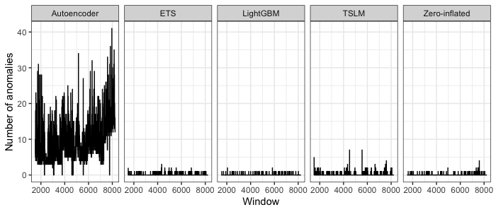
Figure 12: Number of anomalies by hour - autoencoder gives many more anomalies

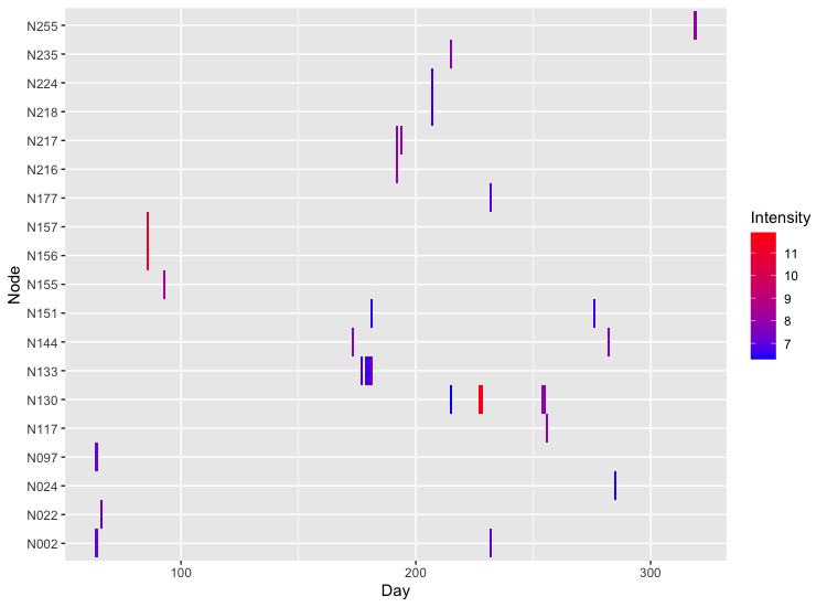
(a)

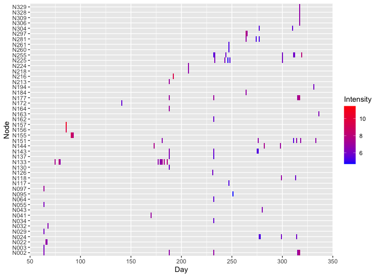
(b)

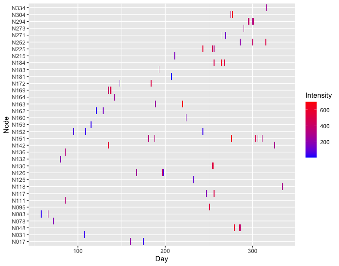
(c)

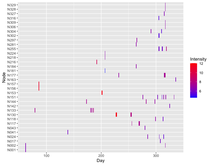
(d)

Figure 13: Anomalies over time using ETS, TSLM, LightGBM and Zero-inflated models

Table 3 gives the number of anomalous nodes identified by each method per hour. We see that the true anomalies occur within only 45 hourly blocks. For the remaining 6660 hours, there are no anomalies. Furthermore, the maximum number of true anomalous nodes in any given hour is 3. All four hierarchical models, ETS, TSLM, LightGBM and the Zero-inflated models do not identify anomalies for a large number of hourly blocks (6448, 6061, 6599 and 6569). The autoencoder, on the other hand, has only 81 hourly blocks without a single anomaly, finding anomalies in the other 6624 hourly blocks, compared to 257, 644, 106 and 136 for ETS, TSLM, LightGBM and Zero-inflated models respectively.

Figure 13 gives a graphical representation of anomalies over time identified by the 4 forecasting models, reconciled by BU method. The horizontal axis denotes the day and the vertical axis lists the anomalous nodes found by each method. When a node is found anomalous on a given day, it is shown by a small vertical line. The colour of the line depicts the logarithm of absolute residual values as the range of the residual values is large. Some nodes such as N133 and N151 appear multiple times with the span of days signifying that these nodes need to be investigated. A graphical representation can aid with such decision making when the false positives are low. We see that generally ETS+lookout produces a smaller number of anomalous nodes compared to the other 3 methods. Furthermore, there are not many anomalies between day 100 to 150. In contrast, we see many anomalies between day 200 and 300.

Table 3: Anomaly frequency by method per hour

Method	Anomaly Frequency Stats
	Zeros	Non-zeros	Q0.5	Q0.75	Q0.95	Max
ETS-lookout	6448	257	0	0	0	3
TSLM-lookout	6061	644	0	0	1	7
LightGBM	6599	106	0	0	0	2
Zero-inflated	6569	136	0	0	0	4
Autoencoder	81	6624	7	11	19	41
True anomalies	6660	45	0	0	0	3

5 Discussion and Conclusion

We have presented a forecasting-based approach that uses information from across the network for detecting anomalous behaviour inside a LAN. Due to firewalls and NADs being situated at the external gateway, anomalies inside a LAN tend to be rarer compared to anomalies in external traffic. Therefore, we need methods that produce low false positives and don’t render the system meaningless. Our proposed approach comprises of forecasting ARP calls for each node by using hierarchical forecasting methods to extract information from across the network, and detecting anomalies using the forecast errors. We have used four forecasting methods – ETS, TSLM, LightGBM and Zero-inflated – and three forecast reconciliation methods – BU, TD and MinT – as part of the hierarchical forecasting framework. We used an extreme value theory based anomaly detection method called lookout to find anomalous behaviour. As a comparison, we used an autoencoder on hourly ARP calls to detect anomalies and reported the results.

The results show that LightGBM with lookout is the best combination for anomaly detection. LightGBM is a machine learning forecasting method and has achieved the highest F-measure and precision values in this work. The Zero-inflated model and TSLM are the next best options. We did not observe a significant difference between the three forecast reconciliation techniques with respect to anomaly detection, with all three techniques producing nearly identical anomaly detection results. The forecast reconciliation helped to make a better forecast by extracting information from across the network. The main advantage of our approach is that it models the general system and detects deviations at node level while using information from the entire network. Thus, heterogeneous behaviour is accounted for. As an extreme value theory based method is used for anomaly detection, the false positives are low. As shown in Figure 13 and Table 3 the number of anomalies identified per day is much smaller compared to an autoencoder. This can make a real difference in a security expert’s work life.

The current framework considered time series forecasting as one component and the anomaly detection as a separate component. We did not consider any feedback between the two components. That is, in a given time window all the data was used to train the forecast models. A design consideration for future research is to modify the training data for the next round according to the predictions of the anomaly detection module in this round. For example, if certain ARP calls are declared anomalous these could be removed from the training data for the next round. However, there is an element of uncertainty in any anomaly detector, and there is a possibility that non-anomalous data is removed, in which case the forecasts would not reflect the true behaviour of the network. As the inner-LAN anomalies are extremely rare (anomalies appear only in 45 windows from a total of 6705 windows), we have not gone down this path. However, this is an avenue for exploration. Another path for future research is to construct an ensemble approach. We have explored 4 time series forecasting models with 3 forecast reconciliation techniques. Different methods are better at forecasting in different instances. Combining these methods in an ensemble forecast can improve the accuracy.

This work aims to consolidate computational techniques that generally belong to two different research communities: the cyber security researchers and the forecasters. While traditional time-series forecasting methods are statistical-based, more machine learning methods are making headway in this space. In fact, as previously noted, LightGBM is a machine learning forecasting method that has achieved considerable success in various forecasting competitions. Notwithstanding this development, time series forecasting methods are still underutilised (or so we think) in cyber security research. We expect this work to contribute to bridge this gap and provide a framework for future research in this direction.

Supplementary material

The data and the programming scripts are available at https://github.com/sevvandi/supplementary_material/tree/master/forecasting_and_anomaly_detection.

References

- (1)
- Abolghasemi et al. (2022a) Mahdi Abolghasemi, Rob J Hyndman, Evangelos Spiliotis, and Christoph Bergmeir. 2022a. Model selection in reconciling hierarchical time series.
- Abolghasemi et al. (2022b) Mahdi Abolghasemi, Garth Tarr, and Christoph Bergmeir. 2022b. Machine learning applications in hierarchical time series forecasting: Investigating the impact of promotions.
- Almohannadi et al. (2018) Hamad Almohannadi, Irfan Awan, Jassim Al Hamar, Andrea Cullen, Jules Pagan Disso, and Lorna Armitage. 2018. Cyber threat intelligence from honeypot data using elasticsearch. In Proceedings - International Conference on Advanced Information Networking and Applications, AINA, Vol. 2018-May. 900–906. https://doi.org/10.1109/AINA.2018.00132
- Balogh et al. (2018) Zoltán Balogh, Štefan Koprda, and Jan Francisti. 2018. LAN security analysis and design. In 2018 IEEE 12th International Conference on Application of Information and Communication Technologies (AICT). IEEE, 1–6.
- Ban et al. (2021) Tao Ban, Ndichu Samuel, Takeshi Takahashi, and Daisuke Inoue. 2021. Combat Security Alert Fatigue with AI-Assisted Techniques. In ACM International Conference Proceeding Series. 9–16. https://doi.org/10.1145/3474718.3474723
- Baykara and Das (2018) Muhammet Baykara and Resul Das. 2018. A novel honeypot based security approach for real-time intrusion detection and prevention systems. Journal of Information Security and Applications 41 (2018), 103–116. https://doi.org/10.1016/j.jisa.2018.06.004
- Bernacki and Kołaczek (2015) Jarosław Bernacki and Grzegorz Kołaczek. 2015. Anomaly detection in network traffic using selected methods of time series analysis. International Journal of Computer Network and Information Security 7, 9 (2015), 10–18.
- Carrier et al. (2022) Tristan Carrier, Princy Victor, Ali Tekeoglu, and Arash Lashkari. 2022. Detecting Obfuscated Malware using Memory Feature Engineering. 177–188. https://doi.org/10.5220/0010908200003120
- Chirupphapa et al. (2022) Pawissakan Chirupphapa, Hiroshi Esaki, and Hideya Ochiai. 2022. Feature Extraction Pipeline and Analysis of Suspicious Events in Large-Scale LANs for Cyberattack Categorization. In Proceedings of the 4th International Conference on Big Data Engineering. 104–112.
- Coles et al. (2001) Stuart Coles, Joanna Bawa, Lesley Trenner, and Pat Dorazio. 2001. An introduction to statistical modeling of extreme values. Vol. 208. Springer.
- Cox et al. (2016) Jacob H. Cox, Russell J. Clark, and Henry L. Owen. 2016. Leveraging SDN for ARP security. In SoutheastCon 2016. 1–8. https://doi.org/10.1109/SECON.2016.7506644
- Cui et al. (2019) Mingjian Cui, Jianhui Wang, and Meng Yue. 2019. Machine learning-based anomaly detection for load forecasting under cyberattacks. IEEE Transactions on Smart Grid 10, 5 (2019), 5724–5734.
- Evangelou and Adams (2020) Marina Evangelou and Niall M Adams. 2020. An anomaly detection framework for cyber-security data.
- Furnell and Thomson (2009) Steven Furnell and Kerry Lynn Thomson. 2009. Recognising and addressing ’security fatigue’. Computer Fraud and Security 2009, 11 (2009), 7–11. https://doi.org/10.1016/S1361-3723(09)70139-3
- Garg and Maheshwari (2016) Akash Garg and Prachi Maheshwari. 2016. Performance analysis of snort-based intrusion detection system. In 2016 3rd international conference on advanced computing and communication systems (icaccs), Vol. 1. IEEE, 1–5.
- GhasemiGol et al. (2016) Mohammad GhasemiGol, Abbas Ghaemi-Bafghi, and Hassan Takabi. 2016. A comprehensive approach for network attack forecasting.
- Hawkins (1980) Douglas M Hawkins. 1980. Identification of outliers. Vol. 11. Springer.
- Hernández-Campos et al. (2004) Félix Hernández-Campos, J. S. Marron, Gennady Samorodnitsky, and F. D. Smith. 2004. Variable heavy tails in Internet traffic. Performance Evaluation 58, 2-3 (2004), 261–284. https://doi.org/10.1016/j.peva.2004.07.008
- Hignam et al. (2021) Kate Hignam, Kai Arulkumaran, Zachary Hanif, and Jennings Nicholas R. 2021. BETH Dataset: Real Cybersecurity Data for Anomaly Detection Research. In ICML Workshop on Uncertainty and Robustness in Deep Learning 2021 and Conference on Applied Machine Learning for Information Security. ICML2021.
- Hyndman and Athanasopoulos (2021) Rob J Hyndman and George Athanasopoulos. 2021. Forecasting: principles and practice (3rd ed.). Melbourne, Australia. http://OTexts.com/fpp3
- IBM Security (2020) IBM Security. 2020. Cost of a Data Breach Report.
- Juba et al. (2013) Yutaka Juba, Hung-Hsuan Huang, and Kyoji Kawagoe. 2013. Dynamic isolation of network devices using OpenFlow for keeping LAN secure from intra-LAN attack. Procedia computer science 22 (2013), 810–819.
- Kandanaarachchi and Hyndman (2022) Sevvandi Kandanaarachchi and Rob J Hyndman. 2022. Leave-One-Out Kernel Density Estimates for Outlier Detection. Journal of Computational and Graphical Statistics 31, 2 (2022), 586–599. https://doi.org/10.1080/10618600.2021.2000425
- Kandanarrchchi et al. (2022) Sevvandi Kandanarrchchi, Hideya Ochiai, and Asha Rao. 2022. Honeyboost: Boosting honeypot performance with data fusion and anomaly detection. Expert Systems with Applications 201 (2022).
- Karakate et al. (2021) Meatasit Karakate, Hiroshi Esaki, and Hideya Ochiai. 2021. SDNHive: A Proof-of-Concept SDN and Honeypot System for Defending Against Internal Threats. In 2021 the 11th International Conference on Communication and Network Security. 9–20.
- Khamphakdee et al. (2014) Nattawat Khamphakdee, Nunnapus Benjamas, and Saiyan Saiyod. 2014. Improving intrusion detection system based on snort rules for network probe attack detection. In 2014 2nd International Conference on Information and Communication Technology (ICoICT). IEEE, 69–74.
- Khraisat et al. (2019) Ansam Khraisat, Iqbal Gondal, Peter Vamplew, and Joarder Kamruzzaman. 2019. Survey of intrusion detection systems: techniques, datasets and challenges. Cybersecurity 2, 1 (2019), 1–22.
- Kiravuo et al. (2013) Timo Kiravuo, Mikko Sarela, and Jukka Manner. 2013. A survey of Ethernet LAN security. IEEE Communications Surveys & Tutorials 15, 3 (2013), 1477–1491.
- L (2018) Wilkinson L. 2018. “Visualizing Big Data Outliers Through Distributed Aggregation,”. IEEE Transactions on Visualization and Computer Graphics 24 (2018), 256.
- Landauer et al. (2018) Max Landauer, Markus Wurzenberger, Florian Skopik, Giuseppe Settanni, and Peter Filzmoser. 2018. Dynamic log file analysis: An unsupervised cluster evolution approach for anomaly detection.
- Li and Liu (2010) Hui Li and Dihua Liu. 2010. Research on intelligent intrusion prevention system based on snort. In 2010 International conference on computer, mechatronics, control and electronic engineering, Vol. 1. IEEE, 251–253.
- Li et al. (2011) Li Li, Hua Sun, and Zhenyu Zhang. 2011. The research and design of honeypot system applied in the LAN security. In 2011 IEEE 2nd International Conference on Software Engineering and Service Science. IEEE, 360–363.
- McKeown et al. (2008) Nick McKeown, Tom Anderson, Hari Balakrishnan, Guru Parulkar, Larry Peterson, Jennifer Rexford, Scott Shenker, and Jonathan Turner. 2008. OpenFlow: enabling innovation in campus networks. ACM SIGCOMM computer communication review 38, 2 (2008), 69–74.
- Moustafa and Slay (2015) Nour Moustafa and Jill Slay. 2015. UNSW-NB15: a comprehensive data set for network intrusion detection systems (UNSW-NB15 network data set). In 2015 Military Communications and Information Systems Conference (MilCIS). 1–6. https://doi.org/10.1109/MilCIS.2015.7348942
- Nam et al. (2010) Seung Yeob Nam, Dongwon Kim, and Jeongeun Kim. 2010. Enhanced ARP: preventing ARP poisoning-based man-in-the-middle attacks. IEEE communications letters 14, 2 (2010), 187–189.
- Ochiai (2018) Hideya Ochiai. 2018. LAN-security monitoring project. IEICE Technical Report; IEICE Tech. Rep. 120, 19 (2018), 27–38.
- Ramaswami et al. (2014) Vaidyanathan Ramaswami, Kaustubh Jain, Rittwik Jana, and Vaneet Aggarwal. 2014. Modeling heavy tails in traffic sources for network performance evaluation. Advances in Intelligent Systems and Computing 246 (2014), 23–44. https://doi.org/10.1007/978-81-322-1680-3_4
- Roesch et al. (1999) Martin Roesch et al. 1999. Snort: Lightweight intrusion detection for networks.. In Lisa, Vol. 99. 229–238.
- Roumani et al. (2015) Yaman Roumani, Joseph K Nwankpa, and Yazan F Roumani. 2015. Time series modeling of vulnerabilities.
- Spiliotis et al. (2021) Evangelos Spiliotis, Mahdi Abolghasemi, Rob J Hyndman, Fotios Petropoulos, and Vassilios Assimakopoulos. 2021. Hierarchical forecast reconciliation with machine learning.
- Sun et al. (2020) Yuwei Sun, Hiroshi Esaki, and Hideya Ochiai. 2020. Adaptive intrusion detection in the networking of large-scale LANs with segmented federated learning. IEEE Open Journal of the Communications Society 2 (2020), 102–112.
- Talagala et al. (2021) Priyanga Dilini Talagala, Rob J. Hyndman, and Kate Smith-Miles. 2021. Anomaly Detection in High-Dimensional Data. Journal of Computational and Graphical Statistics 30, 2 (2021), 360–374. https://doi.org/10.1080/10618600.2020.1807997 arXiv:1908.04000
- Whalen (2001) Sean Whalen. 2001. An introduction to ARP spoofing. Node99 [Online Document] (2001).
- Wickramasuriya et al. (2019) Shanika L Wickramasuriya, George Athanasopoulos, and Rob J Hyndman. 2019. Optimal forecast reconciliation for hierarchical and grouped time series through trace minimization. J. Amer. Statist. Assoc. 114, 526 (2019), 804–819.
- Withers (2022) S. Withers. 2022. Optus breach casts spotlight on cyber resilience. Computer Weekly (2022).
- Yasasin et al. (2020) Emrah Yasasin, Julian Prester, Gerit Wagner, and Guido Schryen. 2020. Forecasting IT security vulnerabilities–An empirical analysis.
- Zhang et al. (2020) Zhiqing Zhang, Pawissakan Chirupphapa, Hiroshi Esaki, and Hideya Ochiai. 2020. XGBoosted misuse detection in LAN-internal traffic dataset. In 2020 IEEE International Conference on Intelligence and Security Informatics (ISI). IEEE, 1–6.