A Majorization-Minimization Gauss-Newton Method for 1-Bit Matrix Completion

Abstract

In 1-bit matrix completion, the aim is to estimate an underlying low-rank matrix from a partial set of binary observations. We propose a novel method for 1-bit matrix completion called MMGN. Our method is based on the majorization-minimization (MM) principle, which yields a sequence of standard low-rank matrix completion problems in our setting. We solve each of these sub-problems by a factorization approach that explicitly enforces the assumed low-rank structure and then apply a Gauss-Newton method. Our numerical studies and application to a real-data example illustrate that MMGN outputs comparable if not more accurate estimates, is often significantly faster, and is less sensitive to the spikiness of the underlying matrix than existing methods.

Keywords: Binary observations, Maximum likelihood estimate, Low-rank matrix, Constrained least squares.

1 Introduction

Consider the following 1-bit matrix completion problem: Let ${\bm{\mathbf{{\Theta}}}}^{*}\in\mathbb{R}^{m\times n}$ be an unknown matrix of exact rank $r^{*}$. The observed data are a subset $\Omega\subset[m]\times[n]$ and a binary matrix ${\bm{\mathbf{{Y}}}}$ whose entries are given by

$${y}_{ij} = \begin{cases}+1&\text{with probability }\Phi({\theta}_{ij}^{*}),\\ -1&\text{with probability }1-\Phi({\theta}_{ij}^{*}),\end{cases}$$ (1)

for $(i,j)\in\Omega$, where $\Phi:\mathbb{R}\rightarrow[0,1]$ is a known cumulative distribution function (CDF). We code missing entries with zero, i.e., $y_{ij}=0$ for $(i,j)\not\in\Omega$. Given the set $\Omega$, the function $\Phi$, and the matrix ${\bm{\mathbf{{Y}}}}$, the 1-bit matrix completion problem is to estimate the underlying matrix ${\bm{\mathbf{{\Theta}}}}^{*}$, see for example Davenport et al. (2014).

This problem is a variant of the classical matrix completion problem, in which one directly observes the entries $\theta_{ij}^{*}$ for $(i,j)\in\Omega$. Indeed, in some applications, one can only observe some stochastic value $y_{ij}$ that is non-linearly related to the underlying value $\theta_{ij}^{*}$. For example, in the Netflix challenge, a famous collaborative filtering task, the goal was to predict the missing entries of a ratings matrix whose observed entries were integers ranging from one to five. In the simplest model for recommendation systems, user responses take only two values: “like” or “dislike”, leading to a 1-bit matrix completion problem. Additional applications involving completion of partially observed binary matrices include incomplete survey data (Miller, 1956) and quantum state tomography (Gross et al., 2010).

Assumptions are needed on both the underlying matrix ${\bm{\mathbf{{\Theta}}}}^{*}$ and the subset $\Omega$ of observed entries to ensure that this 1-bit matrix completion problem is well-posed. Intuitively, the matrix ${\bm{\mathbf{{\Theta}}}}^{*}$ needs to be de-localized, or not overly “spiky”, so that the observed entries provide sufficient information to accurately estimate all of ${\bm{\mathbf{{\Theta}}}}^{*}$. Here, we adopt the notion of matrix spikiness from Negahban and Wainwright (2012). For a non-zero matrix ${\bm{\mathbf{{\Theta}}}}\in\mathbb{R}^{m\times n}$, its spikiness ratio $s({\bm{\mathbf{{\Theta}}}})$ is defined as

$$s({\bm{\mathbf{{\Theta}}}}) = \sqrt{mn}\frac{\lVert{\bm{\mathbf{{\Theta}}}}\lVert_{\infty}}{\lVert{\bm{\mathbf{{\Theta}}}}\lVert_{\text{F}}},$$

where $\lVert{\bm{\mathbf{{\Theta}}}}\rVert_{\infty}=\max_{ij}|\theta_{i,j}|$ and $\lVert{\bm{\mathbf{{\Theta}}}}\rVert_{\text{F}}$ is its Frobenius norm. By definition, the spikiness ratio satisfies $1\leq s({\bm{\mathbf{{\Theta}}}})\leq\sqrt{mn}$. In general, a lower value of $s({\bm{\mathbf{{\Theta}}}}^{*})$ yields an easier 1-bit matrix completion problem. Spikiness is less restrictive than the notion of matrix incoherence (Candès and Recht, 2009; Candes and Plan, 2010; Keshavan et al., 2010) used in the matrix completion literature. For a comparison between spikiness and incoherence, we refer the reader to Negahban and Wainwright (2012).

In addition to the matrix ${\bm{\mathbf{{\Theta}}}}^{*}$ having a low spikiness value, the set $\Omega$ of observed entries needs to be well spread-out. Several previous works assumed that $\Omega$ is distributed uniformly at random. For a sufficiently large $|\Omega|$, this enables accurate estimation of ${\bm{\mathbf{{\Theta}}}}^{*}$, see for example Bhaskar and Javanmard (2015), Davenport et al. (2014), and Cai and Zhou (2013).

In this work, we implicitly assume that the set $\Omega$ is sufficiently large and spread-out and that the underlying matrix is not overly spiky. We focus on the computational challenge of estimating ${\bm{\mathbf{{\Theta}}}}^{*}$. Given the observed entries of ${\bm{\mathbf{{Y}}}}$, perhaps the most natural approach to estimate ${\bm{\mathbf{{\Theta}}}}^{*}$ is by maximizing the likelihood function, or equivalently minimizing the negative log-likelihood $\ell({\bm{\mathbf{{\Theta}}}})$ under a rank-$r$ constraint,

$$\underset{{\bm{\mathbf{{\Theta}}}}\in\mathbb{R}^{m\times n}}{\text{minimize}}\;\ell({\bm{\mathbf{{\Theta}}}})\quad\text{subject to}\quad\text{rank}({\bm{\mathbf{{\Theta}}}})\mathop{\>\>\,}\nolimits\leq\mathop{\>\>\,}\nolimits r.$$ (2)

Specifically, under the model in (1), the negative log-likelihood of the 1-bit matrix completion problem is given by

$$\ell({\bm{\mathbf{{\Theta}}}}) = -\sum_{(i,j)\in\Omega}\bigg{\{}{\delta}_{ij}\log\Phi({\theta}_{ij})+(1-{\delta}_{ij})\log\left[1-\Phi({\theta}_{ij})\right]\bigg{\}},$$ (3)

where $\delta_{ij}=\frac{1}{2}(1+{y}_{ij})$.

Several authors developed algorithms as well as corresponding theoretical error bounds for the 1-bit matrix completion problem. Instead of directly solving (2), several previous methods added a constraint of the form $\|{\bm{\mathbf{{\Theta}}}}\|_{\infty}\leq\alpha$, where $\alpha$ is a tuning parameter. For example, Davenport et al. (2014) replaced the nonconvex rank constraint with a constraint on the trace norm $\lVert{\bm{\mathbf{{\Theta}}}}\lVert_{*}$ which is the sum of the singular values of ${\bm{\mathbf{{\Theta}}}}$. Their modified convex problem is

$$\underset{{\bm{\mathbf{{\Theta}}}}\in\mathbb{R}^{m\times n}}{\text{minimize}}\;\ell({\bm{\mathbf{{\Theta}}}})\quad\text{subject to}\quad\lVert{\bm{\mathbf{{\Theta}}}}\lVert_{*}\mathop{\>\,}\nolimits\leq\mathop{\>\,}\nolimits\alpha\beta\sqrt{mn}\quad\text{and}\quad\lVert{\bm{\mathbf{{\Theta}}}}\lVert_{\infty}\mathop{\>\,}\nolimits\leq\mathop{\>\,}\nolimits\alpha,$$ (4)

which depends on two tuning parameters $\alpha$ and $\beta$.

Instead of the trace norm, Cai and Zhou (2013) employed the max-norm (Linial et al., 2007) as a convex relaxation of the rank. For a matrix ${\bm{\mathbf{{\Theta}}}}$, its max-norm is defined as $\lVert{\bm{\mathbf{{\Theta}}}}\lVert_{\text{max}}=\min_{{\bm{\mathbf{{\Theta}}}}={\bm{\mathbf{{U}}}}{\bm{\mathbf{{V}}}}^{\sf T}}\{\lVert{\bm{\mathbf{{U}}}}\lVert_{2,\infty},\lVert{\bm{\mathbf{{V}}}}\lVert_{2,\infty}\}$, where $\lVert{\bm{\mathbf{{U}}}}\lVert_{2,\infty}$ is the largest $l_{2}$-norm of the rows in ${\bm{\mathbf{{U}}}}$. They estimated the underlying matrix ${\bm{\mathbf{{\Theta}}}}^{*}$ by solving

$$\underset{{\bm{\mathbf{{\Theta}}}}\in\mathbb{R}^{m\times n}}{\text{minimize}}\;\ell({\bm{\mathbf{{\Theta}}}})\quad\text{subject to}\quad\lVert{\bm{\mathbf{{\Theta}}}}\lVert_{\max}\mathop{\>\,}\nolimits\leq\mathop{\>\,}\nolimits\alpha\beta\quad\text{and}\quad\lVert{\bm{\mathbf{{\Theta}}}}\lVert_{\infty}\mathop{\>\,}\nolimits\leq\mathop{\>\,}\nolimits\alpha.$$

Bhaskar and Javanmard (2015) and Ni and Gu (2016) developed factorization-based algorithms for solving the nonconvex problem with the original rank constraint, though still with an additional constraint on $\|{\bm{\mathbf{{\Theta}}}}\|_{\infty}$,

$$\underset{{\bm{\mathbf{{\Theta}}}}\in\mathbb{R}^{m\times n}}{\text{minimize}}\;\ell({\bm{\mathbf{{\Theta}}}})\quad\text{subject to}\quad\text{rank}({\bm{\mathbf{{\Theta}}}})\mathop{\>\,}\nolimits\leq\mathop{\>\,}\nolimits r\quad\text{and}\quad\left\lVert{\bm{\mathbf{{\Theta}}}}\right\rVert_{\infty}\mathop{\>\,}\nolimits\leq\mathop{\>\,}\nolimits\alpha.$$

The above works also derived error bounds for the global minimizers of their respective objectives. For example, Davenport et al. (2014, Theorem 1) provided the following error bound: Assume ${\bm{\mathbf{{\Theta}}}}^{*}\in\mathbb{R}^{n\times n}$ is approximately low rank in the sense that $\|{\bm{\mathbf{{\Theta}}}}^{*}\|_{*}\leq\alpha n\sqrt{r^{*}}$, further assume $\|{\bm{\mathbf{{\Theta}}}}^{*}\|_{\infty}\leq\alpha$, and that entries in $\Omega$ are sampled according to a uniform distribution with $|\Omega|$ sufficiently large. Then, with high probability,

$$\frac{1}{n^{2}}\left\lVert\hat{{\bm{\mathbf{{\Theta}}}}}-{\bm{\mathbf{{\Theta}}}}^{*}\right\lVert_{\text{F}}^{2} \leq C\sqrt{{\frac{r^{*}n}{|\Omega|}}},$$ (5)

for some constant $C$. Cai and Zhou (2013) considered a more general sampling model and derived an error bound for their estimator, which is of the same order as in (5).

The primary contribution of this manuscript is the development of a novel, simple, and computationally fast approach for solving problem (2). From a computational perspective, most existing methods for 1-bit matrix completion are quite complicated, and as we will see in Section 3, they are all relatively slow. Our method assumes that the rank $r^{*}$ of ${\bm{\mathbf{{\Theta}}}}^{*}$ is known, but we also present a data-driven method to estimate it, when it is unknown. Our iterative method, Majorization-Minimization Gauss-Newton (MMGN), is simple to implement and only requires solving a sequence of linear least squares problems. Hence, it can easily scale to large matrices. Our numerical experiments demonstrate that MMGN is typically at least an order of magnitude faster than existing methods, while achieving the same, or sometimes even better, estimation accuracy. This is notable particularly in the case of spikier matrices.

The rest of the paper is organized as follows. Section 2 introduces the MMGN method. Sections 3 and 4 present an empirical evaluation of MMGN with simulation experiments and a real data application. Section 5 concludes with a discussion.

Notation. We denote vectors by boldface lowercase letters and matrices by boldface capital letters, e.g., ${\bm{\mathbf{{a}}}}\in\mathbb{R}^{n}$ and ${\bm{\mathbf{{A}}}}\in\mathbb{R}^{m\times n}$. We denote the entries of a vector ${\bm{\mathbf{{a}}}}$ and matrix ${\bm{\mathbf{{A}}}}$ by ${a}_{i}$ and ${a}_{ij}$, respectively. The rank of a matrix ${\bm{\mathbf{{A}}}}$ is denoted by $\text{rank}({\bm{\mathbf{{A}}}})$, its Moore–Penrose pseudo inverse by ${\bm{\mathbf{{A}}}}^{\dagger}$, and its column-major vectorization, i.e., the vector obtained by stacking the columns of ${\bm{\mathbf{{A}}}}$ one after the other, by $\text{vec}({\bm{\mathbf{{A}}}})$. We will frequently use the following semi-norm of a matrix ${\bm{\mathbf{{A}}}}$, denoted by $\lVert{\bm{\mathbf{{A}}}}\rVert_{\text{F}(\Omega)}=\sqrt{\sum_{(i,j)\in\Omega}a_{ij}^{2}}$, where $\Omega$ is a subset of ${\bm{\mathbf{{A}}}}$’s indices. Similarly, for a vector ${\bm{\mathbf{{a}}}}$, we denote the semi-norm $\lVert{\bm{\mathbf{{a}}}}\rVert_{\Omega}=\sqrt{\sum_{i\in\Omega}a_{i}^{2}}$, where $\Omega$ is a subset of ${\bm{\mathbf{{a}}}}$’s indices. For two matrices ${\bm{\mathbf{{A}}}}$ and ${\bm{\mathbf{{B}}}}$ of the same size, we denote the Hadamard product as ${\bm{\mathbf{{A}}}}\circ{\bm{\mathbf{{B}}}}$, namely $({\bm{\mathbf{{A}}}}\circ{\bm{\mathbf{{B}}}})_{ij}={a}_{ij}{b}_{ij}$. Similarly, the element-wise quotient of ${\bm{\mathbf{{A}}}}$ and ${\bm{\mathbf{{B}}}}$ is ${\bm{\mathbf{{A}}}}\oslash{\bm{\mathbf{{B}}}}$, namely $({\bm{\mathbf{{A}}}}\oslash{\bm{\mathbf{{B}}}})_{ij}={a}_{ij}/{b}_{ij}$. For a set $S$, we denote its cardinality as $|S|$. Finally, for any univariate function $\Phi:\mathbb{R}\rightarrow\mathbb{R}$, we denote the matrix obtained by applying $\Phi$ entry-wise to ${\bm{\mathbf{{A}}}}$ by $\Phi({\bm{\mathbf{{A}}}})$.

2 The MMGN Method

We first overview our approach. Our strategy for solving the nonconvex problem (2) is based on the majorization-minimization (MM) principle. Concretely, we replace the objective function $\ell({\bm{\mathbf{{\Theta}}}})$ with a simpler surrogate function, called a majorization. As we show below, minimizing our majorization leads to a standard low-rank matrix completion problem. Hence, MMGN solves a sequence of optimization problems of the form

$$\underset{{\bm{\mathbf{{\Theta}}}}\in\mathbb{R}^{m\times n}}{\text{minimize}}\;\left\lVert{\bm{\mathbf{{\Theta}}}}-{\bm{\tilde{\mathbf{{Y}}}}}\right\rVert_{\text{F}(\Omega)}^{2}\quad\quad\text{subject to}\quad\quad\text{rank}({\bm{\mathbf{{\Theta}}}})\mathop{\>\,}\nolimits\leq\mathop{\>\,}\nolimits r,$$ (6)

where ${\bm{\tilde{\mathbf{{Y}}}}}$ is a matrix that depends on the observed entries of the data matrix ${\bm{\mathbf{{Y}}}}$ and the current estimate ${\bm{\tilde{\mathbf{{\Theta}}}}}$.

We solve (6) by a factorization approach, expressing ${\bm{\mathbf{{\Theta}}}}={\bm{\mathbf{{U}}}}{\bm{\mathbf{{V}}}}^{\sf T}$ where ${\bm{\mathbf{{U}}}}\in\mathbb{R}^{m\times r}$ and ${\bm{\mathbf{{V}}}}\in\mathbb{R}^{n\times r}$. Therefore, we rewrite (6) as the following equivalent unconstrained problem

$$\underset{{\bm{\mathbf{{U}}}}\in\mathbb{R}^{m\times r},{\bm{\mathbf{{V}}}}\in\mathbb{R}^{n\times r}}{\text{minimize}}\;\left\lVert{\bm{\mathbf{{U}}}}{\bm{\mathbf{{V}}}}^{\sf T}-{\bm{\tilde{\mathbf{{Y}}}}}\right\rVert_{\text{F}(\Omega)}^{2}.$$ (7)

Finally, we solve (7) using a modified Gauss-Newton algorithm introduced by Zilber and Nadler (2022).

2.1 The Majorization-Minimization Principle

The MM principle (De Leeuw, 1994; Heiser, 1995; Lange et al., 2000; Hunter and Lange, 2004; Lange, 2016) converts minimizing a challenging function $\ell({\bm{\mathbf{{\Theta}}}})$ into solving a sequence of simpler optimization problems. The idea is to approximate an objective function $\ell({\bm{\mathbf{{\Theta}}}})$ to be minimized by a surrogate function or majorization $g({\bm{\mathbf{{\Theta}}}}\mid{\bm{\tilde{\mathbf{{\Theta}}}}})$ anchored at the current estimate ${\bm{\tilde{\mathbf{{\Theta}}}}}$. The majorization $g({\bm{\mathbf{{\Theta}}}}\mid{\bm{\tilde{\mathbf{{\Theta}}}}})$ needs to satisfy two conditions: (i) a tangency condition $g({\bm{\tilde{\mathbf{{\Theta}}}}}\mid{\bm{\tilde{\mathbf{{\Theta}}}}})=\ell({\bm{\tilde{\mathbf{{\Theta}}}}})$ for all ${\bm{\tilde{\mathbf{{\Theta}}}}}$ and (ii) a domination condition $g({\bm{\mathbf{{\Theta}}}}\mid{\bm{\tilde{\mathbf{{\Theta}}}}})\geq\ell({\bm{\tilde{\mathbf{{\Theta}}}}})$ for all ${\bm{\mathbf{{\Theta}}}}$. The associated MM algorithm is defined by the iterates

$${\bm{\mathbf{{\Theta}}}}_{t+1} = \operatorname*{arg\,min}_{{\bm{\mathbf{{\Theta}}}}}g({\bm{\mathbf{{\Theta}}}}\mid{\bm{\mathbf{{\Theta}}}}_{t}),~{}~{}~{}t=0,1,\dots.$$ (8)

The tangency and domination conditions imply that

$$\ell({\bm{\mathbf{{\Theta}}}}_{t+1})~{}~{}\leq~{}~{}g({\bm{\mathbf{{\Theta}}}}_{t+1}\mid{\bm{\mathbf{{\Theta}}}}_{t})~{}~{}\leq~{}~{}g({\bm{\mathbf{{\Theta}}}}_{t}\mid{\bm{\mathbf{{\Theta}}}}_{t})~{}~{}=~{}~{}\ell({\bm{\mathbf{{\Theta}}}}_{t}).$$

In other words, the sequence of objective function values of the MM iterates decreases monotonically. Finding the global minimizer of $g({\bm{\mathbf{{\Theta}}}}\mid{\bm{\mathbf{{\Theta}}}}_{t})$ is not necessary to ensure the descent property. Therefore, one can inexactly solve (8) and still guarantee a monotonic decrease of the objective. The key to successfully applying the MM principle is to construct a surrogate function that is easy to minimize.

Recall that we seek to minimize the negative log-likelihood of the 1-bit matrix completion problem (3), which we restate here for convenience:

$$\ell({\bm{\mathbf{{\Theta}}}}) = -\sum_{(i,j)\in\Omega}\bigg{\{}{\delta}_{ij}\log\Phi({\theta}_{ij})+(1-{\delta}_{ij})\log\left[1-\Phi({\theta}_{ij})\right]\bigg{\}},$$

where $\delta_{ij}=\frac{1}{2}(1+{y}_{ij})\in\{0,1\}$ are rescalings of the observed entries. To derive our majorization, we assume the CDF $\Phi(\theta)$ in (3) satisfies the following two conditions.

• The function $\log\Phi(\theta)$ is $L$-Lipschitz differentiable.

• The density function $\phi(\theta)=\Phi^{\prime}(\theta)$ is symmetric around zero. This implies that $\Phi(\theta)=1-\Phi(-\theta)$.

The following proposition describes a quadratic majorization under the above assumptions.

Proposition 2.1.

Let $\Phi(\theta)$ be a CDF that satisfies assumptions A1 and A2. The following is a majorization of $\ell({\bm{\mathbf{{\Theta}}}})$ at ${\bm{\tilde{\mathbf{{\Theta}}}}}$

$$g({\bm{\mathbf{{\Theta}}}}\mid{\bm{\tilde{\mathbf{{\Theta}}}}}) = \frac{L}{2}\left\lVert{\bm{\mathbf{{\Theta}}}}-{\bm{\tilde{\mathbf{{Y}}}}}\right\rVert_{\text{F}(\Omega)}^{2}+c({\bm{\tilde{\mathbf{{\Theta}}}}}),$$ (9)

where $c({\bm{\tilde{\mathbf{{\Theta}}}}})$ is a constant that depends on ${\bm{\tilde{\mathbf{{\Theta}}}}}$ but not on ${\bm{\mathbf{{\Theta}}}}$, and

$${\bm{\tilde{\mathbf{{Y}}}}} = {\bm{\tilde{\mathbf{{\Theta}}}}}+\frac{1}{L}\left({\bm{\mathbf{{Y}}}}\circ\phi({\bm{\tilde{\mathbf{{\Theta}}}}})\right)\oslash\Phi\left({\bm{\mathbf{{Y}}}}\circ{\bm{\tilde{\mathbf{{\Theta}}}}}\right).$$ (10)

Two popular CDFs in 1-bit matrix completion are $\Phi(x)=1/(1+e^{-x/\sigma})$ and $\Phi(x)=\frac{1}{\sqrt{2\pi\sigma^{2}}}\int_{-\infty}^{x}\exp\left(-\frac{w^{2}}{2\sigma^{2}}\right)dw$, which correspond to logistic and Gaussian random variables, respectively. Both satisfy assumptions A1 and A2. Hence, by Proposition 2.1 we obtain the following specific quadratic majorizations.

Corollary 2.1.

Under the logistic model with $\Phi(x)=1/(1+e^{-x/\sigma})$, the following is a majorization of $\ell({\bm{\mathbf{{\Theta}}}})$ at ${\bm{\tilde{\mathbf{{\Theta}}}}}$

$$g({\bm{\mathbf{{\Theta}}}}\mid{\bm{\tilde{\mathbf{{\Theta}}}}}) = \frac{1}{8\sigma^{2}}\left\lVert{\bm{\mathbf{{\Theta}}}}-{\bm{\tilde{\mathbf{{Y}}}}}\right\rVert_{\text{F}(\Omega)}^{2}+c_{1},$$

where $c_{1}$ is a constant that does not depend on ${\bm{\mathbf{{\Theta}}}}$ and

$${\bm{\tilde{\mathbf{{Y}}}}} = {\bm{\tilde{\mathbf{{\Theta}}}}}+4\sigma{\bm{\mathbf{{Y}}}}\circ\Phi\left(-{\bm{\mathbf{{Y}}}}\circ{\bm{\tilde{\mathbf{{\Theta}}}}}\right).$$

Corollary 2.2.

Under the probit model with $\Phi(x)=\frac{1}{\sqrt{2\pi\sigma^{2}}}\int_{-\infty}^{x}\exp\left(-\frac{w^{2}}{2\sigma^{2}}\right)dw$, the following is a majorization of $\ell({\bm{\mathbf{{\Theta}}}})$ at ${\bm{\tilde{\mathbf{{\Theta}}}}}$

$$g({\bm{\mathbf{{\Theta}}}}\mid{\bm{\tilde{\mathbf{{\Theta}}}}}) = \frac{1}{2\sigma^{2}}\left\lVert{\bm{\mathbf{{\Theta}}}}-{\bm{\tilde{\mathbf{{Y}}}}}\right\rVert_{\text{F}(\Omega)}^{2}+c_{2},$$

where $c_{2}$ is a constant that does not depend on ${\bm{\mathbf{{\Theta}}}}$ and

$${\bm{\tilde{\mathbf{{Y}}}}} = {\bm{\tilde{\mathbf{{\Theta}}}}}+\sigma^{2}{\bm{\mathbf{{Y}}}}\circ\phi({\bm{\tilde{\mathbf{{\Theta}}}}})\oslash\Phi({\bm{\mathbf{{Y}}}}\circ{\bm{\tilde{\mathbf{{\Theta}}}}}).$$

Proofs of Proposition 2.1, Corollary 2.1, and Corollary 2.2 are in the supplementary materials. The two corollaries indicate that both the logistic and probit models lead to MM-updates that require solving a standard low-rank matrix completion problem.

$$\underset{{\bm{\mathbf{{\Theta}}}}\in\mathbb{R}^{m\times n}}{\text{minimize}}\;\left\lVert{\bm{\mathbf{{\Theta}}}}-{\bm{\tilde{\mathbf{{Y}}}}}\right\rVert_{\text{F}(\Omega)}^{2}\quad\quad\text{subject to}\quad\quad\text{rank}({\bm{\mathbf{{\Theta}}}})\mathop{\>\>\,}\nolimits\leq\mathop{\>\>\,}\nolimits r.$$ (11)

We denote the solution to the problem (11) by ${\bm{\mathbf{{\Theta}}}}_{\text{MM}}$. We next review how we approximately solve problem (11) by a Gauss-Newton strategy.

2.2 Inexact Majorization-Minimization via Gauss-Newton

Let $g({\bm{\mathbf{{\Theta}}}}\mid{\bm{\tilde{\mathbf{{\Theta}}}}})$ be a quadratic majorization of the form (9) with ${\bm{\tilde{\mathbf{{Y}}}}}$ defined in (10), where ${\bm{\tilde{\mathbf{{\Theta}}}}}$ denotes our current estimate of ${\bm{\mathbf{{\Theta}}}}$. It is useful to express $g({\bm{\mathbf{{\Theta}}}}\mid{\bm{\tilde{\mathbf{{\Theta}}}}})$ in terms of the difference ${\bm{\mathbf{{\Theta}}}}-{\bm{\tilde{\mathbf{{\Theta}}}}}$. The MM-update in (11) can then be written as

$${\bm{\mathbf{{\Theta}}}}_{\text{MM}} = \underset{\textrm{rank}({\bm{\mathbf{{\Theta}}}})\leq r}{\arg\min}\;g({\bm{\mathbf{{\Theta}}}}|{\bm{\tilde{\mathbf{{\Theta}}}}})\mathop{\>\>\,}\nolimits=\mathop{\>\>\,}\nolimits\underset{\textrm{rank}({\bm{\mathbf{{\Theta}}}})\leq r}{\arg\min}\;\left\lVert{\bm{\mathbf{{\Theta}}}}-{\bm{\tilde{\mathbf{{\Theta}}}}}-{\bm{\mathbf{{X}}}}\right\rVert_{\text{F}(\Omega)}^{2},$$ (12)

where

$${\bm{\mathbf{{X}}}} = {\bm{\tilde{\mathbf{{Y}}}}}-{\bm{\tilde{\mathbf{{\Theta}}}}}\mathop{\>\>\,}\nolimits=\mathop{\>\>\,}\nolimits\frac{1}{L}{\bm{\mathbf{{Y}}}}\circ\phi({\bm{\tilde{\mathbf{{\Theta}}}}})\oslash\Phi\left({\bm{\mathbf{{Y}}}}\circ{\bm{\tilde{\mathbf{{\Theta}}}}}\right).$$ (13)

This results in the following factorization approach for solving (12). We express ${\bm{\tilde{\mathbf{{\Theta}}}}}$ and ${\bm{\mathbf{{\Theta}}}}$ as the product of two rank-$r$ factor matrices with

$${\bm{\tilde{\mathbf{{\Theta}}}}} = \tilde{{\bm{\mathbf{{U}}}}}\tilde{{\bm{\mathbf{{V}}}}}^{\sf T}\quad\quad\text{and}\quad\quad{\bm{\mathbf{{\Theta}}}}\mathop{\>\>\,}\nolimits=\mathop{\>\>\,}\nolimits\left({\bm{\tilde{\mathbf{{U}}}}}+\Delta{\bm{\mathbf{{U}}}}\right)\left(\tilde{{\bm{\mathbf{{V}}}}}+\Delta{\bm{\mathbf{{V}}}}\right)^{\sf T}.$$

The variables ${\bm{\tilde{\mathbf{{U}}}}}\in\mathbb{R}^{m\times r}$ and ${\bm{\tilde{\mathbf{{V}}}}}\in\mathbb{R}^{n\times r}$ are the factor matrices corresponding to the current estimate ${\bm{\tilde{\mathbf{{\Theta}}}}}$, whereas $\Delta{\bm{\tilde{\mathbf{{U}}}}}\in\mathbb{R}^{m\times r}$ and $\Delta{\bm{\tilde{\mathbf{{V}}}}}\in\mathbb{R}^{n\times r}$ are their updates. Therefore, problem (12) can be written in terms of the new variables ($\Delta{\bm{\mathbf{{U}}}}$, $\Delta{\bm{\mathbf{{V}}}}$) as

$$\underset{\Delta{\bm{\mathbf{{U}}}},\Delta{\bm{\mathbf{{V}}}}}{\text{minimize}}\;\left\lVert{\bm{\mathbf{{X}}}}-\tilde{{\bm{\mathbf{{U}}}}}\Delta{\bm{\mathbf{{V}}}}^{\sf T}-\Delta{\bm{\mathbf{{U}}}}\tilde{{\bm{\mathbf{{V}}}}}^{\sf T}-\Delta{\bm{\mathbf{{U}}}}\Delta{\bm{\mathbf{{V}}}}^{\sf T}\right\rVert_{\text{F}(\Omega)}^{2}.$$ (14)

The optimization problem in (14) is a nonlinear least squares problem. Motivated by Zilber and Nadler (2022), we employ a single step of the Gauss-Newton method and neglect the second order term $\Delta{\bm{\mathbf{{U}}}}\Delta{\bm{\mathbf{{V}}}}^{\sf T}$. We thus compute the solution ($\Delta{\bm{\mathbf{{U}}}}^{*}$, $\Delta{\bm{\mathbf{{V}}}}^{*}$) to

$$\underset{\Delta{\bm{\mathbf{{U}}}},\Delta{\bm{\mathbf{{V}}}}}{\text{minimize}}\;\left\lVert{\bm{\mathbf{{X}}}}-\tilde{{\bm{\mathbf{{U}}}}}\Delta{\bm{\mathbf{{V}}}}^{\sf T}-\Delta{\bm{\mathbf{{U}}}}\tilde{{\bm{\mathbf{{V}}}}}^{\sf T}\right\rVert_{\text{F}(\Omega)}^{2}.$$ (15)

Ignoring the second order term in (14) approximates the nonlinear least squares problem with the linear least squares problem in (15). This yields the following inexact solution of (12), denoted $\hat{{\bm{\mathbf{{\Theta}}}}}_{\text{MM}}$,

$$\hat{{\bm{\mathbf{{\Theta}}}}}_{\text{MM}} = \;\;\left(\tilde{{\bm{\mathbf{{U}}}}}+\Delta{\bm{\mathbf{{U}}}}^{*}\right)\left(\tilde{{\bm{\mathbf{{V}}}}}+\Delta{\bm{\mathbf{{V}}}}^{*}\right)^{\sf T}.$$ (16)

We address three important details about our approach. The first is that the linear least squares problem in (15) has infinitely many solutions. For example, suppose that $(\Delta{\bm{\mathbf{{U}}}}^{*},\Delta{\bm{\mathbf{{V}}}}^{*})$ is a solution to (15), then $(\Delta{\bm{\mathbf{{U}}}}^{*}+{\bm{\tilde{\mathbf{{U}}}}}{\bm{\mathbf{{R}}}},\Delta{\bm{\mathbf{{V}}}}^{*}-{\bm{\tilde{\mathbf{{V}}}}}{\bm{\mathbf{{R}}}}^{\sf T})$ is also a solution to (15) for any ${\bm{\mathbf{{R}}}}\in\mathbb{R}^{r\times r}$. Here we adopt the strategy used by Bauch et al. (2021) and Zilber and Nadler (2022) and select the least $l_{2}$-norm solution to the problem, namely the pair $(\Delta{\bm{\mathbf{{U}}}}^{*},\Delta{\bm{\mathbf{{V}}}}^{*})$ with smallest norm $\lVert\Delta{\bm{\mathbf{{U}}}}^{*}\rVert_{\text{F}}^{2}+\lVert\Delta{\bm{\mathbf{{V}}}}^{*}\rVert_{\text{F}}^{2}$ among all pairs of $(\Delta{\bm{\mathbf{{U}}}}^{*},\Delta{\bm{\mathbf{{V}}}}^{*})$ that solve (15). This solution can be computed efficiently using the LSQR algorithm (Paige and Saunders, 1982).

The second detail is that the update in (16) may not necessarily lead to a decrease in the objective function. The Gauss-Newton method is an instance of the steepest descent algorithm, and consequently the solution pair $(\Delta{\bm{\mathbf{{U}}}}^{*},\Delta{\bm{\mathbf{{V}}}}^{*})$ corresponds to a descent direction. The update in (16), however, corresponds to a full Gauss-Newton step which may not necessarily decrease the value of the original objective function in (12). To overcome this potential problem, if the updated solution $\hat{{\bm{\mathbf{{\Theta}}}}}_{\text{MM}}$ in (16) does not decrease the original objective, we apply the Armijo backtracking line search to select a suitable stepsize instead of applying a full Gauss-Newton step (Nocedal and Wright, 2006, Chapter 3). In our experience, however, the backtracking line search is seldom triggered in practice. Details on this and a discussion on the convergence of MMGN are in the supplementary materials.

The third detail is that there is no need to globally minimize the majorization (12). Motivated by computational considerations, we inexactly solve the MM optimization problem by taking a single Gauss-Newton step. This differs from the approach of Zilber and Nadler (2022), which solves (15) using multiple iteration steps and is thus more computationally intensive. Inexact minimization is a standard approach in cases where exact minimization requires an iterative solver. See, for example, the split-feasibility algorithm in Xu et al. (2018), which also employed a single Gauss-Newton step. Under suitable regularity conditions, little is lost by a single-step MM-gradient approach. Not only does it avoid potentially expensive inner iterations within outer MM iterations, it often exhibits the same local convergence rate as exact minimization (Hunter and Lange, 2004).

Algorithm 1 MMGN

1:$\Omega$, ${\bm{\mathbf{{Y}}}}$, target rank $r$, tolerance tol

2:Initialize ${\bm{\mathbf{{U}}}}_{0}$, ${\bm{\mathbf{{V}}}}_{0}$, set $t=0$, $\mathrm{rel}=\texttt{INF}$

3:while $\mathrm{rel}>\texttt{tol}$ do

4:     Construct ${\bm{\mathbf{{X}}}}_{t}$ in (13) as $\triangleright$ Majorization

$${\bm{\mathbf{{X}}}}_{t} = \frac{1}{L}{\bm{\mathbf{{Y}}}}\circ\phi\left({\bm{\mathbf{{U}}}}_{t}{\bm{\mathbf{{V}}}}_{t}^{\sf T}\right)\oslash\Phi\left({\bm{\mathbf{{Y}}}}\circ\left({\bm{\mathbf{{U}}}}_{t}{\bm{\mathbf{{V}}}}_{t}^{\sf T}\right)\right).$$

5:     Compute the least $l_{2}$-norm solution $(\Delta{\bm{\mathbf{{U}}}}^{*},\Delta{\bm{\mathbf{{V}}}}^{*})$ to $\triangleright$ Single MM-gradient step

$$\underset{\Delta{\bm{\mathbf{{U}}}},\Delta{\bm{\mathbf{{V}}}}}{\text{minimize}}\;\left\lVert{\bm{\mathbf{{X}}}}_{t}-{\bm{\mathbf{{U}}}}_{t}\Delta{\bm{\mathbf{{V}}}}^{\sf T}-\Delta{\bm{\mathbf{{U}}}}{\bm{\mathbf{{V}}}}_{t}^{\sf T}\right\rVert_{\text{F}(\Omega)}^{2}.$$

6:     Update factor matrices

$$\begin{bmatrix}{\bm{\mathbf{{U}}}}_{t+1}\\ {\bm{\mathbf{{V}}}}_{t+1}\\ \end{bmatrix} = \begin{bmatrix}{\bm{\mathbf{{U}}}}_{t}\\ {\bm{\mathbf{{V}}}}_{t}\end{bmatrix}+\alpha_{t}\begin{bmatrix}\Delta{\bm{\mathbf{{U}}}}^{*}\\ \Delta{\bm{\mathbf{{V}}}}^{*}\end{bmatrix},$$

where $\alpha_{t}$ is a stepsize parameter chosen via the Armijo backtracking line search.

7:     Compute the relative change in the log-likelihood

$$\mathrm{rel} = \frac{|\ell({\bm{\mathbf{{U}}}}_{t+1}{\bm{\mathbf{{V}}}}_{t+1}^{\sf T})-\ell({\bm{\mathbf{{U}}}}_{t}{\bm{\mathbf{{V}}}}_{t}^{\sf T})|}{|\ell({\bm{\mathbf{{U}}}}_{t}{\bm{\mathbf{{V}}}}_{t}^{\sf T})|}.$$

8:     $t=t+1$.

9:end while

10:return $\hat{{\bm{\mathbf{{\Theta}}}}}={\bm{\mathbf{{U}}}}_{t}{\bm{\mathbf{{V}}}}_{t}^{\sf T}$.

3 Numerical Experiments

We present simulation studies that compare the performance of MMGN to the following two methods: TraceNorm (Davenport et al., 2014) and MaxNorm (Cai and Zhou, 2013). Specifically, we use the computationally more efficient version of TraceNorm that omits the infinity norm constraint in (4). Although Davenport et al. (2014) required the constraint $\lVert{\bm{\mathbf{{\Theta}}}}\lVert_{\infty}\leq\alpha$ to establish their error bound, they observed that omitting it did not significantly affect the estimation performance and moreover simplified the optimization problem. We implemented MMGN in MATLAB . We employed MATLAB implementations of TraceNorm and MaxNorm provided by their respective authors. The methods in Bhaskar and Javanmard (2015) and Ni and Gu (2016) have no publicly available code and consequently were not included in our comparisons.

In all our simulations, we assume that the rank of the underlying matrix is unknown. For MMGN, we use the following validation approach to estimate the rank $r$ in (2). Given a candidate set of $K$ ranks $\{r_{1},\cdots,r_{K}\}$, we randomly split the observations into a training set (80%) and a validation set (20%). For each candidate rank $r_{k}$, we compute an estimate $\hat{{\bm{\mathbf{{\Theta}}}}}_{k}$ using the training set and then calculate the likelihood at $\hat{{\bm{\mathbf{{\Theta}}}}}_{k}$ on the validation set. We select the candidate rank which produces the greatest likelihood among all $K$ candidates as our estimate of the rank $r$. For TraceNorm and MaxNorm, we set the parameter $\alpha$ to its oracle value $\lVert{\bm{\mathbf{{\Theta}}}}^{*}\lVert_{\infty}$ and set $\beta$ to $\sqrt{r}$, where $r$ is estimated using the same validation approach employed in MMGN. Even with a given rank $r$, TraceNorm and MaxNorm may output a matrix with a higher rank. Consequently, we compute a truncated rank-$r$ SVD on their outputs to return a rank-$r$ matrix.

Given a target rank $r$, we set parameters of the compared methods as follows: (1) For TraceNorm, all algorithmic parameters were set to their default values in the provided code. (2) For MaxNorm, the rank parameter in their projected gradient algorithm was set to $r+1$ as suggested in Cai and Zhou (2013). A grid of $50$ values evenly spaced between $1$ and $\max(m,n)$ was provided for the stepsize parameter $\tau$. The maximal number of iterations was set to $1000$. (3) For MMGN, the tolerance parameter tol was set to $10^{-4}$. We applied the same stopping rule used in MMGN to MaxNorm. However, MaxNorm is sensitive to the choice of tolerance. Its required tolerance ranges from $10^{-4}$ to $10^{-6}$ to attain convergence.

We evaluate the performance of each method with the following three metrics.

• The relative error $\lVert\hat{{\bm{\mathbf{{\Theta}}}}}-{\bm{\mathbf{{\Theta}}}}^{*}\rVert_{\text{F}}^{2}/\lVert{\bm{\mathbf{{\Theta}}}}^{*}\rVert_{\text{F}}^{2}$.

• The Hellinger distance between the distribution $\Phi(\hat{{\bm{\mathbf{{\Theta}}}}})$ and the true distribution $\Phi({\bm{\mathbf{{\Theta}}}}^{*})$. The Hellinger distance between two matrices ${\bm{\mathbf{{P}}}},{\bm{\mathbf{{Q}}}}\in[0,1]^{m\times n}$ is given by

  $$d_{H}^{2}({\bm{\mathbf{{P}}}},{\bm{\mathbf{{Q}}}}) = \frac{1}{mn}\sum_{i,j}d_{H}^{2}({\bm{\mathbf{{P}}}}_{ij},{\bm{\mathbf{{Q}}}}_{ij}),$$

  where $d_{H}^{2}(p,q)=(\sqrt{p}-\sqrt{q})^{2}+(\sqrt{1-p}-\sqrt{1-q})^{2}$ for $p,q\in[0,1]$.

• The runtime.

In our simulation study, we consider two types of low-rank underlying matrices: non-spiky and spiky. We generate matrices of each type as follows.

• Non-spiky. To generate a non-spiky matrix ${\bm{\mathbf{{\Theta}}}}^{*}\in\mathbb{R}^{m\times n}$ of rank $r^{*}$, we construct ${\bm{\mathbf{{U}}}}^{*}\in\mathbb{R}^{m\times r^{*}}$, ${\bm{\mathbf{{V}}}}^{*}\in\mathbb{R}^{n\times r^{*}}$ with i.i.d. entries from a uniform distribution on $[-0.5,0.5]$. We set ${\bm{\mathbf{{\Theta}}}}^{*}={\bm{\mathbf{{U}}}}^{*}{\bm{\mathbf{{V}}}}^{\sf*T}$ and scale it so that $\|{\bm{\mathbf{{\Theta}}}}^{*}\|_{\infty}=1$. This procedure is the same as Davenport et al. (2014) and Cai and Zhou (2013).

• Spiky. To generate a spiky matrix ${\bm{\mathbf{{\Theta}}}}^{*}\in\mathbb{R}^{m\times n}$ of rank $r^{*}$, we construct ${\bm{\mathbf{{U}}}}^{*}\in\mathbb{R}^{m\times r^{*}}$, ${\bm{\mathbf{{V}}}}^{*}\in\mathbb{R}^{n\times r^{*}}$ with i.i.d. entries from the $t$-distribution with $\nu$ degrees of freedom. We set ${\bm{\mathbf{{\Theta}}}}^{*}={\bm{\mathbf{{U}}}}^{*}{\bm{\mathbf{{V}}}}^{\sf*T}$. We do not rescale ${\bm{\mathbf{{\Theta}}}}^{*}$. A smaller value of $\nu$ yields a heavier-tailed distribution of entries of ${\bm{\mathbf{{\Theta}}}}^{*}$, resulting in a spikier matrix ${\bm{\mathbf{{\Theta}}}}^{*}$.

In each experiment, we first generate an underlying matrix ${\bm{\mathbf{{\Theta}}}}^{*}$ and then the binary matrix ${\bm{\mathbf{{Y}}}}$ according to model (1). We randomly select the set of indices $\Omega$ from a uniform distribution with a user-defined fraction of observed entries $\rho$, namely $\rho=\frac{\lvert\Omega\rvert}{mn}$. We run $20$ replicates for each experimental setting and report the median of the three performance metrics for each method.

3.1 Non-spiky Matrices

Following Davenport et al. (2014) and Cai and Zhou (2013), we first compare the performance of different methods when the underlying matrix is non-spiky. We first consider the probit noise model, where the random noise variables $z_{ij}$ are i.i.d. from $N(0,\sigma^{2})$. As discussed in Davenport et al. (2014), the noise level $\sigma$ is a crucial parameter in 1-bit matrix completion. As $\sigma$ tends to zero, the problem becomes ill-posed, as any two different positive values for $\theta_{ij}^{*}$ yield the same value $y_{ij}=1$. The first experiment studies the sensitivity of different methods to the noise level $\sigma$. We vary $\sigma$ from $10^{-1.25}$ to $10^{0.25}$. We set the matrix dimension $m=n=1000$ and rank $r^{*}=1$. The generated underlying matrices are non-spiky; their average spikiness ratio $s({\bm{\mathbf{{\Theta}}}}^{*})$ is 3.00 with a standard deviation of $0.05$. For each method, we estimate its rank $r$ from $\{1,2,3,4,5\}$, by the validation procedure described earlier.

Figure 1 depicts relative errors, Hellinger distances, and run times (in seconds on a log scale) of the three methods with a fraction of observed entries $\rho=0.8$. The left panel shows that the estimation performance of each method is poor when the noise level is either too low or too high. This corroborates the results in Davenport et al. (2014) and Cai and Zhou (2013). MaxNorm performs well when the noise level is relatively low but struggles more at higher noise levels than MMGN and TraceNorm. In contrast, MMGN and TraceNorm produce poorer estimation at low noise levels. The middle panel displays that all methods exhibit similar trends in the Hellinger distance under varying noise levels as in the relative error. We observe that at $\sigma=10^{-1.25}$, MMGN produces a larger relative error but a lower Hellinger distance, compared to TraceNorm. This discrepancy comes from the nonlinear transformation from ${\bm{\mathbf{{\Theta}}}}^{*}$ to $\Phi({\bm{\mathbf{{\Theta}}}}^{*})$, which we explain later. The right panel shows that run times of MMGN and TraceNorm decrease as the noise level grows, and MMGN is much faster than TraceNorm. MaxNorm, however, requires longer run times when the noise level is either too low or too high. Moreover, MaxNorm runs at least an order of magnitude slower than MMGN and TraceNorm over a wide range of noise levels. In light of these significantly longer run times, we decided in all subsequent experiments to supply MaxNorm with the oracle rank $r^{*}$ instead of estimating it using the validation procedure.

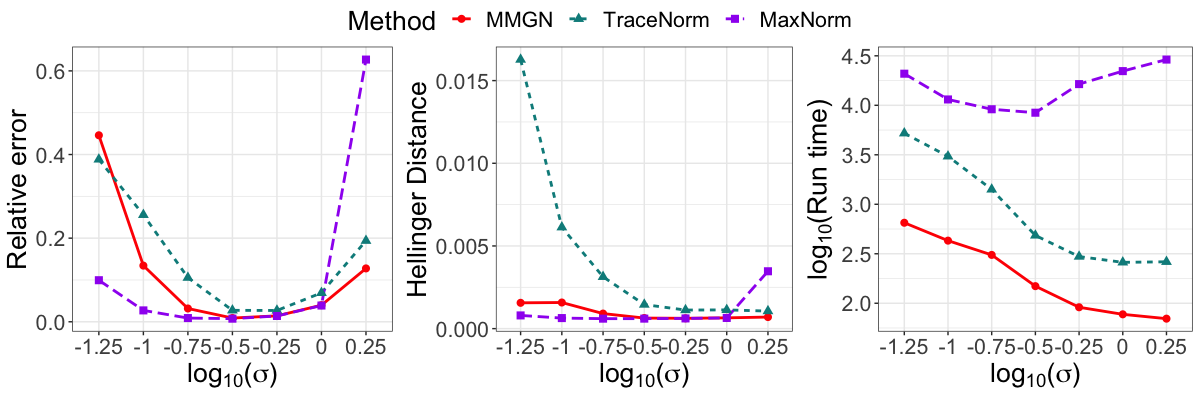
Figure 1: Probit model: Relative error, Hellinger distance, and run time versus noise level $\sigma$ for a non-spiky underlying matrix of size $m\times n=1000\times 1000$ and rank $r^{*}=1$ at a fraction of observed entries $\rho=0.8$.

In our second experiment, we investigate the performance of different methods as a function of the fraction of observed entries $\rho$, in the set $\{0.2,0.3,\ldots,1\}$. The underlying matrices are the same as in the first experiment. We consider both the probit and logistic models with a noise level $\sigma=1$. For MMGN and TraceNorm, we again estimate $r$ from $\{1,2,3,4,5\}$ by the validation procedure described above.

Figure 2: Probit model ($\sigma=1$): Relative error, Hellinger distance, and run time versus fraction of observed entries $\rho$ for a non-spiky underlying matrix of size $m\times n=1000\times 1000$ and rank $r^{*}=1$.

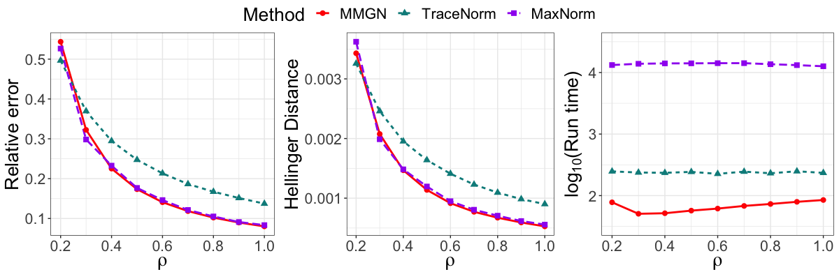
Figure 3: Logistic model ($\sigma=1$): Relative error, Hellinger distance, and run time versus fraction of observed entries $\rho$ for a non-spiky underlying matrix of size $m\times n=1000\times 1000$ and rank $r^{*}=1$.

Figure 4: Log-log plots of relative error versus fraction of observed entries $\rho$ for a non-spiky underlying matrix of size $m\times n=1000\times 1000$ and rank $r^{*}=1$. The left and right plots refer to the experiments summarized in Figure 2 and Figure 3, respectively.

Figure 2 shows simulation results under the probit model. As expected, the estimation errors, as well as the Hellinger distances, of all methods decrease as the fraction of observed entries $\rho$ increases. MMGN and MaxNorm behave comparably and consistently outperform TraceNorm. The right panel displays MMGN’s computational advantage. MMGN requires substantially less time to achieve comparable estimation accuracy with MaxNorm even when MaxNorm enjoys the advantage of employing the oracle rank $r^{*}$. Figure 3 shows the performance of all methods across a range of $\rho$ values under the logistic model. In this experiment, we have to increase the maximum number of iterations of MaxNorm to $3000$ to attain its convergence. MMGN and MaxNorm again achieve comparable estimation accuracy and are modestly better than TraceNorm except for $\rho=0.2$. The right panel of Figure 3 shows that MMGN has a clear advantage in computational speed, particularly over MaxNorm.

Figure 4 displays on a log-log scale the relative errors as a function of $\rho$ under the probit (left panel) and logistic (right panel) models. Under the probit model, all three log-log plots have a slope of approximately $-1$. Namely, all three methods exhibit a better error rate in $\rho$ than the bound in (5). An improved rate also occurs under the logistic noise model. Recall, however, that the error bound in (5) was for approximately low-rank matrices, while our simulated matrices are exactly low-rank.

In the third experiment, we compare the performance of different methods under different matrix dimensions. For simplicity, we consider square underlying matrices, taking $m=n$ and varying $n$ over a grid of values $\{500,1000,1500,2000,2500\}$. We fix the rank of the underlying matrices at $r^{*}=5$. The average spikiness ratios of the generated underlying matrices at the respective dimension scenarios are $\{4.69,4.85,5.02,5.23,5.27\}$. We consider the probit model with $\sigma=0.18$ and fix the fraction of observed entries $\rho=0.8$. For MMGN and TraceNorm, we employ the validation method previously described to estimate their rank $r$ from a candidate set $\{3,4,5,6,7\}$.

Figure 5 shows relative errors, Hellinger distances, and run times of each method under different matrix dimensions. Overall the estimation accuracy of all methods improves as the matrix dimension $n$ grows, with TraceNorm’s accuracy being slightly worse than the other two. The log-log plots on the left panel of Figure 7 indicate that relative errors of all methods scale approximately at a rate of $\mathcal{O}\left(1/n\right)$. The right panel of Figure 5 shows MMGN’s computational advantage over the other two methods. In particular, MMGN is about four times faster than MaxNorm in achieving comparably accurate estimates, even when MaxNorm is given the true rank $r^{*}=5$ and MMGN estimates its rank $r$ from $\{3,4,5,6,7\}$.

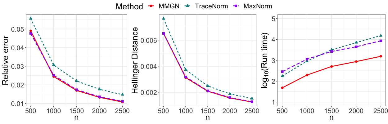
Figure 5: Probit model ($\sigma=0.18$): Relative error, Hellinger distance, and run time versus matrix dimension $n$ for a square non-spiky underlying matrix of size $n\times n$ and rank $r^{*}=5$.

In the last experiment under the non-spiky case, we examine how different methods behave when increasing the rank of the underlying matrix. We fix the size of ${\bm{\mathbf{{\Theta}}}}^{*}$ at $m=n=1000$ and generate matrices of rank $r^{*}\in\{3,5,8,10\}$. The average spikiness ratios of the generated underlying matrices at the respective rank scenarios are $\{4.56,4.85,5.00,5.06\}$. We consider the probit model with a noise level $\sigma=0.18$ and set the fraction of observed entries $\rho=0.8$ for each rank scenario. For MMGN and TraceNorm, we estimate their rank $r$ from $\{3,4,\cdots,10\}$.

Figure 6: Probit model ($\sigma=0.18$): Relative error, Hellinger distance, and run time versus true rank $r^{*}$ for a non-spiky underlying matrix of size $m\times n=1000\times 1000$ and fraction of observed entries $\rho=0.8$.

Figure 7: Log-log plots of relative error versus matrix dimension $n$ (left ) and versus true rank $r^{*}$ (right ). The left and right plots refer to the experiments summarized in Figure 5 and Figure 6, respectively.

Figure 6 displays the performance of different methods under varying rank $r^{*}$. As expected, as $r^{*}$ increases, the estimation accuracy of each method degrades since the number of parameters to be estimated increases. The estimation accuracies of MMGN and MaxNorm are comparable and better than that of TraceNorm. MMGN enjoys the fastest computational speed among the three. Recall that the run time of MMGN includes the time taken to fit multiple models at different ranks to estimate one from the set $\{3,4,\cdots,10\}$, whereas the run time of MaxNorm corresponds to computing its estimate at the single oracle rank $r=r^{*}$. Therefore, the computational advantage of MMGN over MaxNorm is vastly understated in Figure 6. The log-log plots in the right panel of Figure 7 show that relative errors of these three methods scale approximately as $\mathcal{O}\left(r^{*}\right)$.

3.2 Spiky Matrices

We now consider spiky matrices generated by factor matrices ${\bm{\mathbf{{U}}}}^{*}$ and ${\bm{\mathbf{{V}}}}^{*}$ with entries drawn from a heavy-tailed $t$-distribution as described at the beginning of Section 3. Specifically, we consider a square matrix ${\bm{\mathbf{{\Theta}}}}^{*}\in\mathbb{R}^{m\times n}$ with $m=n=1000$ and rank $r^{*}=1$. We set the degrees of freedom $\nu$ to $10$, $5$, and $4$ to generate underlying matrices at low, intermediate, and high spikiness levels. The corresponding average spikiness ratios (with standard deviation in the parenthesis) over $20$ replicates are $16.84~{}(2.15)$, $32.07~{}(4.08)$, and $48.99~{}(5.28)$, respectively. We consider the probit model with a noise level $\sigma=2$. At each spikiness level, we vary the fraction of observed entries $\rho$ over $\{0.2,0.3,\cdots,1\}$. We estimate the rank $r$ of MMGN and TraceNorm from $\{1,2,3,4,5\}$ using the validation procedure. The supplementary materials contain results of the same experiment but with the noise level $\sigma=1$.

Figure 8: Probit model ($\sigma=2$): Relative error, Hellinger distance, and run time versus fraction of observed entries $\rho$ at low (top), intermediate (middle), and high (bottom) spikiness levels for an underlying matrix of size $m\times n=1000\times 1000$ and rank $r^{*}=1$. Average spikiness ratios are $16.84$ (top), $32.07$ (middle), and $48.99$ (bottom).

Figure 8 displays simulation results at the three spikiness levels. The top panel shows that at the low spikiness level, MMGN consistently achieves higher accuracy, in recovering both the underlying matrix ${\bm{\mathbf{{\Theta}}}}^{*}$ and the distribution matrix $\Phi({\bm{\mathbf{{\Theta}}}}^{*})$, than TraceNorm and MaxNorm over different values of $\rho$. At lower fractions of observed entries, when $\rho$ is less than $0.6$, MaxNorm produces smaller estimation errors in recovering ${\bm{\mathbf{{\Theta}}}}^{*}$ in comparison to TraceNorm but larger errors at higher fractions of observed entries, when $\rho$ exceeds $0.6$. However, MaxNorm recovers the underlying distribution more accurately than TraceNorm, as shown in the top middle panel of Figure 8. As in the first experiment in the non-spiky case, this discrepancy between the estimation of ${\bm{\mathbf{{\Theta}}}}^{*}$ and $\Phi({\bm{\mathbf{{\Theta}}}}^{*})$ comes from the nonlinear transformation from ${\bm{\mathbf{{\Theta}}}}^{*}$ to $\Phi({\bm{\mathbf{{\Theta}}}}^{*})$. We give a detailed explanation at the end of this section.

At intermediate and high spikiness levels, MMGN continues to outperform TraceNorm and MaxNorm in estimating ${\bm{\mathbf{{\Theta}}}}^{*}$ and $\Phi({\bm{\mathbf{{\Theta}}}}^{*})$. As the spikiness level grows, MaxNorm consistently achieves better estimation of ${\bm{\mathbf{{\Theta}}}}^{*}$ and $\Phi({\bm{\mathbf{{\Theta}}}}^{*})$, compared to TraceNorm. In general, among the three methods, TraceNorm is the most sensitive to the spikiness level. This sensitivity is reflected in both the estimation accuracy and the required computational time. As the spikiness levels increases, TraceNorm experiences a more pronounced decrease in the estimation accuracy and an increase in the computational time. At the high spikiness level in the bottom row of Figure 8, we excluded the results of TraceNorm for $\rho$ less than $0.4$ because the algorithm failed to converge to an optimal solution for these values of $\rho$. Details on these convergence issues as well as the certificate of optimality used to diagnose them are in the supplementary materials.

An interesting phenomenon is that the errors of estimating ${\bm{\mathbf{{\Theta}}}}^{*}$ using MMGN and MaxNorm are relatively insensitive to $\rho$ at the intermediate and high spikiness levels. Their estimation errors are dominated by errors in the large-magnitude entries. The estimation error of the large-magnitude entries is hardly affected by $\rho$. Both MMGN and MaxNorm produce accurate estimates for the majority of low-magnitude entries, even if $\rho$ is small. Therefore, increasing $\rho$ does not lead to significant improvement in their estimation errors. In contrast, TraceNorm requires a relatively large $\rho$ to produce good estimates for low-magnitude entries. As a result, we see a more noticeable decrease in its estimation error as $\rho$ grows. We use a specific example to elaborate on this phenomenon in the supplementary materials.

The right panel of each row in Figure 8 displays the appealing computational advantage of MMGN when dealing with spiky matrices at different spikiness levels. These results imply that MMGN outperforms existing methods in estimation accuracy and computational speed, even when it estimates its rank in a data-driven manner. Furthermore, the performance gains are most pronounced as the recovery problem becomes harder as the spikiness level of the underlying matrix increases.

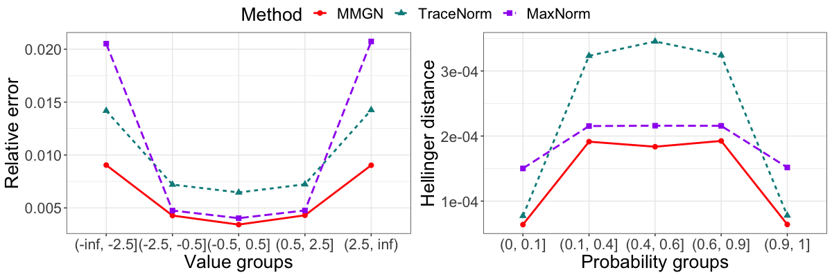
Figure 9: Estimation performance of different methods versus underlying matrix entry values ${\theta}_{ij}$ and probabilities $\Phi({\theta}_{ij})$ for a spiky underlying matrix with the spikiness ratio $s=19.55$.

The experiments so far investigated the overall estimation accuracy, that involves an averaging of the squared errors over all the entries of the matrix. However, a more careful inspection reveals that the three methods have different performance profiles depending on the magnitude of the underlying entries of the matrix ${\bm{\mathbf{{\Theta}}}}^{*}$. To better understand this more fine-grained performance, we study the estimation performance conditioned on the underlying values $\theta_{ij}^{*}$, for a matrix ${\bm{\mathbf{{\Theta}}}}^{*}$ with a low spikiness ratio.

Specifically, we considered an underlying matrix ${\bm{\mathbf{{\Theta}}}}^{*}$ of size $m\times n=1000\times 1000$, rank $r^{*}=1$, and spikiness ratio $s=19.55$. The fraction of observed entries $\rho$ is set to $0.8$. The resulting overall relative errors for MMGN, TraceNorm, and MaxNorm were $0.0301$, $0.0493$, and $0.0548$. The corresponding Hellinger distances are $6.96\times 10^{-4}$, $1.1\times 10^{-3}$, and $9.49\times 10^{-4}$, respectively. We divided entries of ${\bm{\mathbf{{\Theta}}}}^{*}$ into ‘Value groups’, bins or ranges of values that $\theta_{ij}^{*}$ takes on. These ‘Value groups’ have corresponding ‘Probability groups’. For instance, value group $(-\infty,-2.5]$ corresponds to probability group $(0,0.1]$ since $\ \lim_{\theta\to\infty}\Phi(\theta)=0$ and $\Phi(-2.5)\approx 0.1$ under the considered probit model with $\sigma=2$.

Figure 9 shows the estimation performance of each method over the different value and probability groups. As expected, all methods produce good estimates for small-magnitude entries of ${\bm{\mathbf{{\Theta}}}}^{*}$ (absolute values less than or equal to $2.5$) but poorer estimates for large-magnitude entries. MaxNorm suffers from much larger errors in estimating large-magnitude entries, leading to a larger overall relative error than TraceNorm. However, MaxNorm accurately estimates small-magnitude entries leading to accurate recoveries of the corresponding $\Phi(\theta^{*}_{ij})$ and a smaller Hellinger distance. This discrepancy is caused by the nonlinear transformation from $\theta_{ij}^{*}$ to $\Phi(\theta_{ij}^{*})$. For example, $\Phi(0.5)-\Phi(0.4)\approx 0.019$, while $\Phi(3.6)-\Phi(3.5)\approx 0.004$. In other words, the recovered distribution is more sensitive to the accuracy of the recovered $\hat{\theta}_{ij}$ in small-magnitude groups. In comparison, MMGN gives the best accuracy in recovering ${\bm{\mathbf{{\Theta}}}}^{*}$ and $\Phi({\bm{\mathbf{{\Theta}}}}^{*})$ across all the different groups. Figure 9 provides a more detailed picture of how MMGN outperforms existing methods. Moreover, this explains why the trends in estimating ${\bm{\mathbf{{\Theta}}}}^{*}$ (left panel of the first row in Figure 8) do not mirror the trends in estimating $\Phi({\bm{\mathbf{{\Theta}}}}^{*})$ (middle panel of the first row in Figure 8).

We also compared MMGN with a 1-bit tensor completion (1BitTC) method (Wang and Li, 2020) viewing our matrix as a three-way tensor with the third mode having dimension one. While several methods were proposed for binary tensor completion (Li et al., 2018; Aidini et al., 2018; Ghadermarzy et al., 2018; Wang and Li, 2020), we focused on 1BitTC since, to the best of our knowledge, it has the best error rates, as well as publicly available code. Since 1BitTC works with tensors, it is expected to be much slower than methods that work directly with matrices. As shown in the supplementary materials, in addition to being slower, 1BitTC produced higher errors under many scenarios compared with MMGN.

4 Real Data Application

We applied MMGN to the MovieLens (1M) data set, which is larger but otherwise similar to the MovieLens (100K) data set studied in Davenport et al. (2014). The data set is available at http://www.grouplens.org/node/73http://www.grouplens.org/node/73. It contains $100{,}000$ movie ratings from $6{,}040$ users on $3{,}952$ movies, with each rating on a scale from $1$ to $5$. Following Davenport et al. (2014), we convert all ratings to binary observations by comparing each rating to the average rating over all movies. Ratings above the average are encoded as $+1$ and $-1$ otherwise. Following Davenport et al. (2014), we consider the logistic model with $\sigma=1$ and use $95\%$ of the ratings as the training set to estimate ${\bm{\mathbf{{\Theta}}}}^{*}$. The performance is evaluated on the remaining $5\%$ of ratings by checking whether or not the estimate of ${\bm{\mathbf{{\Theta}}}}^{*}$ correctly predicts the sign of the ratings (above or below the average rating). As in our simulation study, we compare the performance of MMGN to TraceNorm and MaxNorm. We follow Davenport et al. (2014) and treat $\alpha\beta$ as a single parameter in TraceNorm, assigning it $10$ values equally spaced on a logarithmic scale between $10^{-0.5}$ to $10$. We ran MMGN with a candidate rank $r$ ranging from $1$ to $10$. Parameters $\alpha$ and $\beta=\sqrt{r}$ in MaxNorm are set the same as in TraceNorm and MMGN. As in Davenport et al. (2014), we select parameter values for each method that lead to the best prediction performance on the separate evaluation set.

Table 1 summarizes the prediction performance and run times of the three methods averaged over $20$ replicates. All three methods achieve comparable prediction accuracy, but MMGN is more than an order of magnitude faster than both TraceNorm and MaxNorm.

Table 1: Performance of different methods on MovieLens (1M) data

Original rating	1 (%)	2 (%)	3 (%)	4 (%)	5 (%)	overall (%)	time (seconds)
TraceNorm	85.0	75.3	53.8	77.6	92.9	75.0	5.7e+4
MaxNorm	78.8	68.8	48.9	77.6	91.8	72.3	7.8e+4
MMGN	82.7	74.0	54.0	75.4	90.7	73.5	5.2e+3

5 Summary and Discussion

Various applications involve partial binary observations of a large matrix, motivating the need for faster algorithms to solve the 1-bit matrix completion problem. In this paper we proposed MMGN, a novel fast and accurate method for this task. Our algorithm employs the MM principle to convert the original challenging optimization problem into a sequence of standard low-rank matrix completion problems. For each MM-update, we apply a factorization strategy to incorporate the low-rank structure, resulting in a nonlinear least squares problem. We then apply a modified Gauss-Newton scheme to compute an inexact MM-update by solving a linear least squares problem. Hence, in comparison to previous works, our method is relatively simple and also does not include a spikiness constraint.

We demonstrated the effectiveness of MMGN on several simulated 1-bit matrix completion problems with two popular 1-bit noise models, and on a real data example. We compared MMGN to TraceNorm (Davenport et al., 2014) and MaxNorm (Cai and Zhou, 2013). Over a broad range of settings, involving non-spiky and spiky matrices, MMGN achieved comparable and in some cases lower errors, while often being significantly faster.

Finally, we note that MMGN bears some similarities with the algorithm proposed by De Leeuw (2006) for logistic principal component analysis (Collins et al., 2001; Schein et al., 2003). While the two problems are different, both MMGN and the method by De Leeuw (2006) are MM algorithms employing the same majorization of the negative log-likelihood. The difference is that the latter minimizes the rank-constrained least squares problem with the SVD. While this approach can be modified to handle missing data simply by filling in missing entries with the appropriate entries of the last MM iterate, the overall procedure requires storing a complete $m$-by-$n$ matrix regardless of the size of $\lvert\Omega\rvert$. In contrast, the storage requirement of MMGN adapts to $\lvert\Omega\rvert$. Specifically, for $\lvert\Omega\rvert\ll mn$, MMGN requires storing $3\lvert\Omega\rvert+(m+n)r$ numbers, since it employs compressed column storage for the observed data and dense storage for only the factor matrices.

Our work raises several interesting directions for further research. On the practical side, it is of interest to extend MMGN to other quantization models, such as movie ratings between 1 and 5. On the theoretical side, an open problem is to prove that under suitable assumptions, and possibly starting from a sufficiently accurate initial guess, MMGN indeed converges to the maximum likelihood solution.

Supplementary Materials

Title:

Supplementary Materials for “A Majorization-Minimization Gauss-Newton Method for 1-Bit Matrix Completion”. (.pdf file)

References

- Aidini et al. (2018) Aidini, A., Tsagkatakis, G., and Tsakalides, P. (2018), “1-bit tensor completion,” Electronic Imaging, 30, 261–1– 261–6.
- Bauch et al. (2021) Bauch, J., Nadler, B., and Zilber, P. (2021), “Rank 2r iterative least squares: Efficient recovery of ill-conditioned low rank matrices from few entries,” SIAM Journal on Mathematics of Data Science, 3, 439–465.