Short-range baryon-baryon potentials in constituent quark model revisited

Abstract

We revisit the short-range baryon-baryon potentials in the flavor SU(3) sector, using the constituent quark model. We employ the color Coulomb, linear confining, and color magnetic forces between two constituent quarks, and solve the three-quark Schrödinger equation using the Gaussian expansion method to evaluate the wave functions of the octet $(N,\Lambda,\Sigma,\Xi)$ and decuplet $(\Delta,\Sigma^{\ast},\Xi^{\ast},\Omega)$ baryons. We then solve the six-quark equation using the resonating group method and systematically calculate equivalent local potentials for the $S$-wave two-baryon systems which reproduce the relative wave functions of two baryons in the resonating group method. As a result, we find that the flavor antidecuplet states with total spin $J=3$, namely, $\Delta\Delta$, $\Delta\Sigma^{\ast}$, $\Delta\Xi^{\ast}$-$\Sigma^{\ast}\Sigma^{\ast}$, and $\Delta\Omega$-$\Sigma^{\ast}\Xi^{\ast}$ systems, have attractive potentials sufficient to generate dibaryon bound states as hadronic molecules. In addition, the $N\Omega$ system with $J=2$ in coupled channels has a strong attraction and forms a bound state. We also make a comparison with the baryon-baryon potentials from lattice QCD simulations and try to understand the behavior of the potentials from lattice QCD simulations.

I Introduction

Understanding the baryon-baryon interactions has been an interesting topic in hadron physics, as they provide important clues to the quark dynamics inside baryons. The nuclear force, being the most extensively studied case, has been investigated through low-energy nucleon-nucleon ($NN$) scattering data and the properties of the $NN$ bound state, i.e., the deuteron. Phenomenological $NN$ potentials, which precisely reproduce the $NN$ data, are known to have a short-range (relative distance $r<$1\text{\,}\mathrm{f}\mathrm{m}$$) repulsive core and medium-range ($$1\text{\,}\mathrm{f}\mathrm{m}$<r<$2\text{\,}\mathrm{f}\mathrm{m}$$) and long-range ($r>$2\text{\,}\mathrm{f}\mathrm{m}$$) attractive parts Machleidt:1989tm . While meson exchanges can explain the medium- and long-range parts of the nuclear force, quark degrees of freedom are expected to be significant in the short range. In fact, constituent quark model calculations indicate that the short-range repulsive core of the nuclear force is governed by two factors Oka:2000wj : the Pauli exclusion principle among valence quarks, and the spin-spin interaction of the quarks that causes the mass splitting between the nucleon and the $\Delta$ baryon. To confirm this scenario in more general cases, studies of baryon-baryon interactions with different quark content are desired.

Recently, due to experimental and numerical developments, much attention has been paid to interactions between two baryons belonging to the octet ($N$, $\Lambda$, $\Sigma$, and $\Xi$) and decuplet ($\Delta$, $\Sigma^{\ast}$, $\Xi^{\ast}$, and $\Omega$). For example, high statistics $\Sigma^{-}p$ and $\Sigma^{+}p$ scattering experiments were performed in Refs. J-PARCE40:2021qxa and J-PARCE40:2022nvq , respectively, and the nuclear $1s$ state of the $\Xi$ hypernucleus ${}^{15}_{\Xi}\mathrm{C}$ was discovered in Ref. Yoshimoto:2021ljs . Both of these provide us with some information on the $N\Sigma$ and $N\Xi$ interactions. In addition to scattering experiments, we can now use lattice quantum chromodynamics (QCD) simulations and relativistic ion collisions to study baryon-baryon interactions. In lattice QCD simulations, we can extract baryon-baryon local potentials directly from the quark-gluon dynamics of QCD using the HAL QCD method Aoki:2012tk , which has been applied to various systems including decuplet baryons, e.g., $\Omega\Omega$ Gongyo:2017fjb , $N\Omega$ HALQCD:2018qyu , and $\Delta\Delta$ (with heavy pion mass) Gongyo:2020pyy . Such baryon-baryon potentials, especially for unstable baryons, are studied through the analysis of the correlation functions for any pair of baryons in relativistic ion collisions ALICE:2020mfd , in which the large number of baryons, together with theoretical predictions for the correlation functions Morita:2019rph , enables a detailed determination of the baryon-baryon interactions. Furthermore, besides phenomenological models, baryon-baryon interactions are now theoretically calculated through chiral effective field theory, in which the degrees of freedom are tied to QCD symmetries and their realization: hyperon-nucleon interactions Haidenbauer:2019boi and interactions involving decuplet baryons Haidenbauer:2017sws , as well as the nuclear force Machleidt:2011zz .

Motivated by these studies, in the present paper we aim to systematically study the baryon-baryon interactions, particularly focusing on the short-range part, by using a precise wave function for baryons composed of three nonrelativistic constituent quarks. In this sense, our study is an extension of the quark model studies in Refs. Oka:1981ri ; Oka:1981rj , but our calculation covers the interactions of any pair of the ground-state baryons, i.e., the octet and decuplet baryons. Similar studies are found in, e.g., Refs. Oka:1986fr ; Goldman:1987ma ; Oka:1988yq ; Wang:1995bg ; Zhang:1997ny ; Li:1999bc ; Li:2000cb ; Fujiwara:2006yh ; Park:2016cmg ; Park:2019bsz . Our study will provide some clues to understand the mechanism that generates attractive/repulsive force suggested in experiments and lattice QCD simulations. Furthermore, because there are more than one hundred channels of the $S$-wave two-baryon systems from the ground-state baryons, we may expect attractive two-baryon potentials that are sufficient to generate dibaryon bound states in the systematic study.

We evaluate the relative wave function of constituent quarks inside each baryon as the solution of the three-quark Schrödinger equation in the Gaussian expansion method Hiyama:2003cu . We take into account the color Coulomb, linear confining, and color magnetic forces between two constituent quarks. Then, we employ the resonating group method (RGM) to calculate the relative wave function of two baryons in $S$ wave. We translate the relative wave function of two baryons into the equivalent local potentials that reproduce the relative wave functions of two baryons in the RGM. Thanks to this approach, we can compare our results with the baryon-baryon local potentials deduced in the lattice QCD simulations, and any research group can utilize the local potentials for further investigations of two-baryon systems.

The paper is organized as follows. In Sec. II we formulate the constituent quark model for one-baryon and two-baryon systems. We also explain the method used to evaluate the equivalent local potentials in this section. Next, in Sec. III we present our numerical results of the baryon-baryon potentials and dibaryon bound states in the present model. Section IV is devoted to the conclusion of the present study.

II Formulation

II.1 Baryons in the Gaussian expansion method

First of all, we construct the wave function of each baryon in the three-body dynamics of constituent quarks.

In the present study, we employ the color Coulomb, linear confining, and color magnetic forces between two constituent quarks. In general, the $i$-th and $j$-th quarks at a distance $r$ interact via the potential

$$V_{ij}(r)=\frac{\vec{\lambda}_{i}}{2}\cdot\frac{\vec{\lambda}_{j}}{2}\left[\frac{\alpha_{ij}}{r}-\frac{3}{4}kr+D-\frac{2\pi\alpha_{\rm ss}}{3}\frac{\vec{\sigma}_{i}\cdot\vec{\sigma}_{j}}{m_{i}m_{j}}\bar{\delta}(r)\right],$$ (1)

where $\vec{\lambda}_{i}$ and $\vec{\sigma}_{i}$ are sets of the Gell-Mann and Pauli matrices, respectively, acting on the $i$-th quark, $\alpha_{ij}$ and $\alpha_{\rm ss}$ are the coupling constants, $k$ is the confining string tension, $D$ is a constant to reproduce the physical baryon masses, $m_{i}$ is the $i$-th constituent quark mass, and $\bar{\delta}(r)$ is a three-dimensional delta-like function

$$\bar{\delta}(r)\equiv\left(\frac{\sigma}{\sqrt{\pi}}\right)^{3}\exp\left(-\sigma^{2}r^{2}\right),$$ (2)

with a range parameter $\sigma$. The coupling constant for the color Coulomb force $\alpha_{ij}$ is assumed to depend on the reduced mass of the $i$-$j$ quark pair in the following form:

$$\alpha_{ij}\equiv\frac{K}{\mu_{ij}},\quad\mu_{ij}\equiv\frac{m_{i}m_{j}}{m_{i}+m_{j}},$$ (3)

where $K$ is a constant. The quark mass dependence of the color Coulomb coupling constant was initially suggested based on a Lattice QCD calculation Kawanai:2011xb and has been employed in a quark model calculation Yoshida:2015tia . We treat $K$, $\alpha_{\rm ss}$, $k$, $\sigma$, and $D$ as model parameters, while keeping the constituent quark mass $m_{i}$ fixed to reproduce the magnetic moments of the proton and $\Lambda$: $m_{u}=m_{d}=$336\text{\,}\mathrm{M}\mathrm{e}\mathrm{V}$$ and $m_{s}=$509\text{\,}\mathrm{M}\mathrm{e}\mathrm{V}$$, as reported by the Particle Data Group ParticleDataGroup:2022pth . Throughout this study we assume isospin symmetry.

Figure 1: Jacobi coordinates of a three-body system.

We apply the potential (1) to the one-baryon system ($B$) in the constituent quark model, in which the internal configurations of three quarks can be described by the Jacobi coordinates shown in Fig. 1. Inside a baryon, owing to the color configuration of constituent quarks, the $i$-th and $j$-th quarks satisfy the following relation:

$$\frac{\vec{\lambda}_{i}}{2}\cdot\frac{\vec{\lambda}_{j}}{2}=-\frac{2}{3}.$$ (4)

Hence, two quarks at a distance $\rho$ inside the baryon $B$ interact via the potential

$$V_{ij}^{(B)}(\rho)=-\frac{2}{3}\frac{\alpha_{ij}}{\rho}+\frac{1}{2}k\rho-\frac{2}{3}D+\frac{4\pi\alpha_{\rm ss}}{9}\frac{\vec{\sigma}_{i}\cdot\vec{\sigma}_{j}}{m_{i}m_{j}}\bar{\delta}(\rho).$$ (5)

Then, the Schrödinger equation for the quarks inside the baryon $B$ in the constituent quark model becomes

$$\left[m_{1}+m_{2}+m_{3}-\frac{1}{2\mu_{B}}\frac{\partial^{2}}{\partial\bm{\lambda}^{2}}-\frac{1}{2\mu_{B}^{\prime}}\frac{\partial^{2}}{\partial\bm{\rho}^{2}}\right.$$

$$\left.\phantom{\frac{1}{\mu_{\lambda}^{(B)}}}+V_{23}^{(B)}(\rho_{1})+V_{31}^{(B)}(\rho_{2})+V_{12}^{(B)}(\rho_{3})\right]\Psi^{(B)}(\bm{\lambda},\bm{\rho})$$

$$=M_{B}\Psi^{(B)}(\bm{\lambda},\bm{\rho}),$$ (6)

where $\Psi^{(B)}(\bm{\lambda},\bm{\rho})$ is the wave function of the relative motion of three quarks in the baryon $B$, $\bm{\lambda}\equiv\bm{\lambda}_{1}$, $\bm{\rho}\equiv\bm{\rho}_{1}$, $M_{B}$ is the mass of the baryon $B$, and

$$\mu_{B}\equiv\frac{m_{1}(m_{2}+m_{3})}{m_{1}+m_{2}+m_{3}},\quad\mu_{B}^{\prime}\equiv\frac{m_{2}m_{3}}{m_{2}+m_{3}}.$$ (7)

In the present study, we focus on the ground-state baryons. Therefore, both the $\lambda$ and $\rho$ modes of the three constituent quarks have zero orbital angular momenta: $l_{\lambda}=l_{\rho}=0$. To describe this, we employ the Gaussian expansion method Hiyama:2003cu for the wave function $\Psi^{(B)}(\bm{\lambda},\bm{\rho})$:

$$\Psi^{(B)}(\bm{\lambda},\bm{\rho})=\sum_{c=1}^{3}\sum_{n=1}^{N}\sum_{n^{\prime}=1}^{N}C_{c,n,n^{\prime}}^{(B)}\exp\left(-\frac{\lambda_{c}^{2}}{r_{n}^{2}}-\frac{\rho_{c}^{2}}{r_{n^{\prime}}^{2}}\right).$$ (8)

Here, the index $c$ specifies the Jacobi coordinates in Fig. 1 and range parameters $r_{n}$ ($n=1$, $\ldots$, $N$) form a geometric progression:

$$r_{n}=r_{\rm min}\times\left(\frac{r_{\rm max}}{r_{\rm min}}\right)^{(n-1)/(N-1)},$$ (9)

where the minimal and maximal ranges, $r_{\rm min}$ and $r_{\rm max}$, respectively, are fixed according to the physical condition of the system. Then, by using the method summarized in Ref. Hiyama:2003cu , we numerically solve the Schrödinger equation (6) and obtain the eigenvector $C_{c,n,n^{\prime}}^{(B)}$ as well as the eigenvalue $M_{B}$.

Table 1: Model parameters for the baryons.

$K$	$184\text{\,}\mathrm{M}\mathrm{e}\mathrm{V}$
$\alpha_{\rm ss}$	$0.785$
$k$	$0.755\text{\,}\mathrm{G}\mathrm{e}\mathrm{V}\mathrm{/}\mathrm{f}\mathrm{m}$
$\sigma$	$3.50\text{\,}\mathrm{f}\mathrm{m}^{-1}$
$D$	$381\text{\,}\mathrm{M}\mathrm{e}\mathrm{V}$
$m_{u}=m_{d}$	$336\text{\,}\mathrm{M}\mathrm{e}\mathrm{V}$ (fixed)
$m_{s}$	$509\text{\,}\mathrm{M}\mathrm{e}\mathrm{V}$ (fixed)

In this study, the model parameters are determined by fitting the ground-state baryon masses. The fitted parameters are listed in Table 1, and the resulting baryon masses are listed in the second column of Table 2, along with their experimental values ParticleDataGroup:2022pth in parenthesis. The convergence of the results is found to be good with the number of the expansion $N=10$ and the ranges $r_{\rm min}=$0.01\text{\,}\mathrm{f}\mathrm{m}$$ and $r_{\rm max}=$2\text{\,}\mathrm{f}\mathrm{m}$$.

Table 2: Properties of the baryons in the present model. The baryon masses reported by the Particle Data Group ParticleDataGroup:2022pth are written in parenthesis.

Baryon	$M_{B}$ [MeV]	$\sqrt{\braket{r_{B}^{2}}}$ [fm]
$N$	950   (939)	0.43
$\Lambda$	1111 (1116)	0.42
$\Sigma$	1180 (1193)	0.44
$\Xi$	1322 (1318)	0.41
$\Delta$	1235 (1232)	0.51
$\Sigma^{\ast}$	1382 (1385)	0.49
$\Xi^{\ast}$	1530 (1533)	0.47
$\Omega$	1679 (1672)	0.45

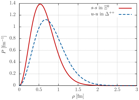
Figure 2: Examples of the density distribution $P(\rho)$.

To evaluate the spatial extension of quarks inside each baryon, we calculate the mean squared radius of the baryon using the formula

$$\braket{r_{B}^{2}}\equiv \frac{1}{3(m_{1}+m_{2}+m_{3})^{2}}\left[(m_{2}+m_{3})^{2}\braket{\lambda_{1}^{2}}\right.$$

$$\quad\left.+(m_{3}+m_{1})^{2}\braket{\lambda_{2}^{2}}+(m_{1}+m_{2})^{2}\braket{\lambda_{3}^{2}}\right],$$ (10)

where $\braket{\lambda_{c}^{2}}$ is the expectation value of $\lambda_{c}^{2}$:

$$\braket{\lambda_{c}^{2}}\equiv\int d^{3}\rho\int d^{3}\lambda\,\lambda_{c}^{2}\left|\Psi^{(B)}(\bm{\lambda},\bm{\rho})\right|^{2}.$$ (11)

The resulting root mean squared radii of baryons, listed in the third column of Table 2, are smaller than the experimental values: for instance, the experimental value of the proton charge radius is about $0.84\text{\,}\mathrm{f}\mathrm{m}$ ParticleDataGroup:2022pth . This discrepancy is attributed to the fact that we only consider the spatial extension of the “quark core” and do not take into account the meson clouds of baryons. It is instructive to show the distribution of quark-quark distance inside the baryons, which we define as

$$P(\rho)=\rho^{2}\int d\Omega_{\rho}\int d^{3}\lambda\left|\Psi^{(B)}(\bm{\lambda},\bm{\rho})\right|^{2}.$$ (12)

Here we choose the distribution of the distance between the $s$-$s$ quarks in the $\Xi^{0}$ baryon and the $u$-$u$ quarks in the $\Delta^{++}$ baryon, because the root mean squared radius $\sqrt{\braket{r_{B}^{2}}}$ of the $\Xi$ baryon has the minimal value $0.41\text{\,}\mathrm{f}\mathrm{m}$, while that of the $\Delta$ baryon has the maximal value $0.51\text{\,}\mathrm{f}\mathrm{m}$. The resulting distribution is shown in Fig. 2 as the solid and dashed lines, respectively. From the figure, we can see that the quark-quark distance in a baryon is about less than $2\text{\,}\mathrm{f}\mathrm{m}$. Because three quarks in a baryon form an almost equilateral triangle, the distribution indicates that the quarks are distributed within a range $\sim(2/\sqrt{3})\,$\mathrm{f}\mathrm{m}$\approx$1.2\text{\,}\mathrm{f}\mathrm{m}$$ from the center of mass of the baryon.

II.2 Two-baryon systems in the resonating group method

II.2.1 Creation and annihilation operators of quarks

Next, we formulate the two-baryon systems in terms of the six-quark degrees of freedom. For this purpose, we introduce creation and annihilation operators of a quark with quantum numbers $\mu\equiv(f,s,c)$, where $f$, $s$, and $c$ represent the flavor, spin, and color, respectively:

$$\hat{a}_{\mu}^{\dagger},\quad\hat{a}_{\mu}.$$ (13)

These operators satisfy the anticommutation relations:

$$\{\hat{a}_{\mu^{\prime}},\hat{a}_{\mu}^{\dagger}\}=\delta_{\mu^{\prime},\mu},\quad\{\hat{a}_{\mu^{\prime}},\hat{a}_{\mu}\}=0,\quad\{\hat{a}_{\mu^{\prime}}^{\dagger},\hat{a}_{\mu}^{\dagger}\}=0.$$ (14)

We also introduce creation and annihilation operators of a quark at the coordinate $\bm{r}$:

$$\hat{b}_{\mu}^{\dagger}(\bm{r}),\quad\hat{b}_{\mu}(\bm{r}),$$ (15)

which satisfy the anticommutation relations:

$$\begin{split}&\{\hat{b}_{\mu^{\prime}}(\bm{r}^{\prime}),\hat{b}_{\mu}^{\dagger}(\bm{r})\}=\delta_{\mu^{\prime},\mu}\delta(\bm{r}^{\prime}-\bm{r}),\\ &\{\hat{b}_{\mu^{\prime}}(\bm{r}^{\prime}),\hat{b}_{\mu}(\bm{r})\}=0,\quad\{\hat{b}_{\mu^{\prime}}^{\dagger}(\bm{r}^{\prime}),\hat{b}_{\mu}^{\dagger}(\bm{r})\}=0.\end{split}$$ (16)

By using the creation operators of quarks, we can express the ket vector of the one-baryon $B$ state as:

$$\ket{B}= \sum_{\vec{\mu}}w_{\vec{\mu}}^{(B)}\int d^{3}r_{1}d^{3}r_{2}d^{3}r_{3}\psi_{1}^{(B)}(\bm{r}_{1})\psi_{2}^{(B)}(\bm{r}_{2})\psi_{3}^{(B)}(\bm{r}_{3})$$

$$\times\hat{b}_{\mu_{1}}^{\dagger}(\bm{r}_{1})\hat{b}_{\mu_{2}}^{\dagger}(\bm{r}_{2})\hat{b}_{\mu_{3}}^{\dagger}(\bm{r}_{3})\ket{0},$$ (17)

where $\vec{\mu}\equiv(\mu_{1},\mu_{2},\mu_{3})$ is the set of the quantum numbers of the three quarks, $w_{\vec{\mu}}^{(B)}$ is the weight for the set $\vec{\mu}$, $\psi_{i}^{(B)}(\bm{r}_{i})$ is the spatial wave function of the $i$-th quark, and $\ket{0}$ is the vacuum. The weight $w_{\vec{\mu}}^{(B)}$ takes, for example $\Delta^{++}$ with the third component of the spin $s=3/2$, value:

$$w_{\vec{\mu}}^{(\Delta^{++}(3/2))}=\begin{cases}1&\vec{\mu}=((u,\uparrow,\mathrm{R}),(u,\uparrow,\mathrm{G}),(u,\uparrow,\mathrm{B})),\\ 0&\text{others}.\end{cases}$$ (18)

We assume that the weight is normalized:

$$\sum_{\vec{\mu}}\left[w_{\vec{\mu}}^{(B)}\right]^{2}=1.$$ (19)

Weights for other baryons are summarized in Table 7 in Appendix. Then, we decompose the product of the spatial wave functions into the center-of-mass part $\Phi^{(B)}(\bm{R})$ with the center-of-mass coordinate $\bm{R}$ and the relative part $\Psi^{(B)}(\bm{\lambda},\bm{\rho})$ as

$$\psi_{1}^{(B)}(\bm{r}_{1})\psi_{2}^{(B)}(\bm{r}_{2})\psi_{3}^{(B)}(\bm{r}_{3})=\Phi^{(B)}(\bm{R})\Psi^{(B)}(\bm{\lambda},\bm{\rho})$$ (20)

where $\bm{R}$, $\bm{\lambda}$, $\bm{\rho}$ are expressed as

$$\begin{split}&\bm{R}\equiv\frac{m_{1}\bm{r}_{1}+m_{2}\bm{r}_{2}+m_{3}\bm{r}_{3}}{m_{1}+m_{2}+m_{3}},\\ &\bm{\lambda}\equiv\bm{r}_{1}-\frac{m_{2}\bm{r}_{2}+m_{3}\bm{r}_{3}}{m_{2}+m_{3}},\quad\bm{\rho}\equiv\bm{r}_{3}-\bm{r}_{2}.\end{split}$$ (21)

Because the measure of the coordinates satisfies the relation

$$d^{3}r_{1}d^{3}r_{2}d^{3}r_{3}=d^{3}Rd^{3}\lambda d^{3}\rho,$$ (22)

we rewrite the ket vector of the one-baryon state as

$$\ket{B}= \int d^{3}R\Phi^{(B)}(\bm{R})\int d^{3}\lambda d^{3}\rho\Psi^{(B)}(\bm{\lambda},\bm{\rho})$$

$$\times\hat{W}^{(B)\dagger}(\bm{r}_{1},\bm{r}_{2},\bm{r}_{3})\ket{0},$$ (23)

where we introduced an operator

$$\hat{W}^{(B)\dagger}(\bm{r}_{1},\bm{r}_{2},\bm{r}_{3})\equiv\sum_{\vec{\mu}}w_{\vec{\mu}}^{(B)}\hat{b}_{\mu_{1}}^{\dagger}(\bm{r}_{1})\hat{b}_{\mu_{2}}^{\dagger}(\bm{r}_{2})\hat{b}_{\mu_{3}}^{\dagger}(\bm{r}_{3}).$$ (24)

Provided the normalization of the wave functions

$$\int d^{3}R\left|\Phi^{(B)}(\bm{R})\right|^{2}=\int d^{3}\lambda d^{3}\rho\left|\Psi^{(B)}(\bm{\lambda},\bm{\rho})\right|^{2}=1,$$ (25)

together with the normalization of the weight (19), the one-baryon vector is normalized:

$$\braket{B}{B}=1.$$ (26)

II.2.2 Hamiltonian

By using the creation and annihilation operators, we can express the Hamiltonian of the system of quarks. The Hamiltonian $\hat{H}$ is composed of the kinetic part $\hat{K}$ and potential part $\hat{V}$:

$$\hat{H}=\hat{K}+\hat{V}.$$ (27)

The kinetic part is expressed as

$$\hat{K}=\sum_{\mu}\int d^{3}r\hat{b}_{\mu}^{\dagger}(\bm{r})\left(m_{f}-\frac{1}{2m_{f}}\frac{\partial^{2}}{\partial\bm{r}^{2}}\right)\hat{b}_{\mu}(\bm{r}),$$ (28)

where $m_{f}$ is the quark mass of the flavor $f$ and the differential operator $\partial^{2}/\partial\bm{r}^{2}$ acts on the wave functions of quarks. The potential part, on the other hand, is composed of the color Coulomb plus linear confining potential and color magnetic potential:

$$\hat{V}=\hat{V}_{\rm CL}+\hat{V}_{\rm ss}.$$ (29)

They are respectively expressed as

$$\hat{V}_{\rm CL}= \frac{1}{2}\sum_{f,f^{\prime},s,s^{\prime}}\int d^{3}r\int d^{3}r^{\prime}V_{\rm CL}(|\bm{r}-\bm{r}^{\prime}|)$$

$$\times\left[\hat{b}^{\dagger}(\bm{r})\frac{\vec{\lambda}}{2}\hat{b}(\bm{r})\right]_{f,s}\cdot\left[\hat{b}^{\dagger}(\bm{r}^{\prime})\frac{\vec{\lambda}}{2}\hat{b}(\bm{r}^{\prime})\right]_{f^{\prime},s^{\prime}},$$ (30)

$$\hat{V}_{\rm ss}= \frac{1}{2}\sum_{f,f^{\prime}}\int d^{3}r\int d^{3}r^{\prime}V_{\rm ss}(|\bm{r}-\bm{r}^{\prime}|)$$

$$\times\left[\hat{b}^{\dagger}(\bm{r})\frac{\vec{\lambda}}{2}\vec{\sigma}\hat{b}(\bm{r})\right]_{f}\cdot\left[\hat{b}^{\dagger}(\bm{r}^{\prime})\frac{\vec{\lambda}}{2}\vec{\sigma}\hat{b}(\bm{r}^{\prime})\right]_{f^{\prime}},$$ (31)

where

$$V_{\rm CL}(r)\equiv\frac{K}{\mu_{ff^{\prime}}r}-\frac{3}{4}kr+D,\quad V_{\rm ss}(r)\equiv-\frac{2\pi\alpha_{\rm ss}}{3m_{f}m_{f^{\prime}}}\bar{\delta}(r),$$ (32)

$$\left[\hat{b}^{\dagger}(\bm{r})\frac{\vec{\lambda}}{2}\hat{b}(\bm{r})\right]_{f,s}\equiv\sum_{c^{\prime},c}\hat{b}_{f,s,c^{\prime}}^{\dagger}(\bm{r})\frac{\vec{\lambda}_{c^{\prime}c}}{2}\hat{b}_{f,s,c}(\bm{r}),$$ (33)

$$\left[\hat{b}^{\dagger}(\bm{r})\frac{\vec{\lambda}}{2}\vec{\sigma}\hat{b}(\bm{r})\right]_{f}\equiv\sum_{s^{\prime},s,c^{\prime},c}\hat{b}_{f,s^{\prime},c^{\prime}}^{\dagger}(\bm{r})\frac{\vec{\lambda}_{c^{\prime}c}}{2}\vec{\sigma}_{s^{\prime}s}\hat{b}_{f,s,c}(\bm{r}).$$ (34)

Then, we can show that the Hamiltonian $\hat{H}$ acting on the ket vector $\ket{B}$ becomes

$$\hat{H}\ket{B}= \int d^{3}R\left(M_{B}-\frac{1}{2M_{B}}\frac{\partial^{2}}{\partial\bm{R}^{2}}\right)\Phi^{(B)}(\bm{R})$$

$$\times\int d^{3}\lambda d^{3}\rho\Psi^{(B)}(\bm{\lambda},\bm{\rho})\hat{W}^{(B)\dagger}(\bm{r}_{1},\bm{r}_{2},\bm{r}_{3})\ket{0},$$ (35)

where we used the Schrödinger equation (6) and the relation of the differential operators

$$\frac{1}{2m_{1}}\frac{\partial^{2}}{\partial\bm{r}_{1}^{2}}+\frac{1}{2m_{2}}\frac{\partial^{2}}{\partial\bm{r}_{2}^{2}}+\frac{1}{2m_{3}}\frac{\partial^{2}}{\partial\bm{r}_{3}^{2}}$$

$$=\frac{1}{2(m_{1}+m_{2}+m_{3})}\frac{\partial^{2}}{\partial\bm{R}^{2}}+\frac{1}{2\mu_{B}}\frac{\partial^{2}}{\partial\bm{\lambda}^{2}}+\frac{1}{2\mu_{B}^{\prime}}\frac{\partial^{2}}{\partial\bm{\rho}^{2}}$$

$$\simeq\frac{1}{2M_{B}}\frac{\partial^{2}}{\partial\bm{R}^{2}}+\frac{1}{2\mu_{B}}\frac{\partial^{2}}{\partial\bm{\lambda}^{2}}+\frac{1}{2\mu_{B}^{\prime}}\frac{\partial^{2}}{\partial\bm{\rho}^{2}}.$$ (36)

In the last line we used an approximation $m_{1}+m_{2}+m_{3}\simeq M_{B}$.

II.2.3 Two-baryon states and the resonating group method

We can straightforwardly extend the ket vector to express the two-baryon $B_{a}B_{b}$ state as

$$\ket{B_{a}B_{b}}= \int d^{3}R_{a}\Phi^{(B_{a})}(\bm{R}_{a})\int d^{3}\lambda_{a}d^{3}\rho_{a}\Psi^{(B_{a})}(\bm{\lambda}_{a},\bm{\rho}_{a})$$

$$\times\int d^{3}R_{b}\Phi^{(B_{b})}(\bm{R}_{b})\int d^{3}\lambda_{b}d^{3}\rho_{b}\Psi^{(B_{b})}(\bm{\lambda}_{b},\bm{\rho}_{b})$$

$$\times\hat{W}^{(B_{a})\dagger}(\bm{r}_{a1},\bm{r}_{a2},\bm{r}_{a3})\hat{W}^{(B_{b})\dagger}(\bm{r}_{b1},\bm{r}_{b2},\bm{r}_{b3})\ket{0}.$$ (37)

In the usual manner, we can decompose the product of the spatial wave functions of the two baryons $\Phi^{(B_{a})}(\bm{R}_{a})\Phi^{(B_{b})}(\bm{R}_{b})$ into the center-of-mass part $\phi(\bm{R}_{\rm tot})$ and the relative part $\psi(\bm{r})$ as

$$\Phi^{(B_{a})}(\bm{R}_{a})\Phi^{(B_{b})}(\bm{R}_{b})=\phi(\bm{R}_{\rm tot})\psi(\bm{r})$$ (38)

with

$$\bm{R}_{\rm tot}\equiv\frac{M_{B_{a}}\bm{R}_{B_{a}}+M_{B_{b}}\bm{R}_{B_{b}}}{M_{B_{a}}+M_{B_{b}}},\quad\bm{r}\equiv\bm{R}_{B_{b}}-\bm{R}_{B_{a}}.$$ (39)

Then we rewrite the two-baryon state as

$$\ket{B_{a}B_{b}}$$

$$=\int d^{3}R_{\rm tot}\phi(\bm{R}_{\rm tot})\int d^{3}r\psi(\bm{r})$$

$$\phantom{=}\times\int d^{3}\lambda_{a}d^{3}\rho_{a}\Psi^{(B_{a})}(\bm{\lambda}_{a},\bm{\rho}_{a})\int d^{3}\lambda_{b}d^{3}\rho_{b}\Psi^{(B_{b})}(\bm{\lambda}_{b},\bm{\rho}_{b})$$

$$\phantom{=}\times\hat{W}^{(B_{a})\dagger}(\bm{r}_{a1},\bm{r}_{a2},\bm{r}_{a3})\hat{W}^{(B_{b})\dagger}(\bm{r}_{b1},\bm{r}_{b2},\bm{r}_{b3})\ket{0},$$ (40)

where we used the relation of the measure

$$d^{3}R_{a}d^{3}R_{b}=d^{3}R_{\rm tot}d^{3}r.$$ (41)

In addition, we introduce the two-baryon vector in which the separation is fixed to be $\bm{r}=\bm{r}_{0}$:

$$\ket{B_{a}B_{b}(\bm{r}_{0})}$$

$$=\int d^{3}R_{\rm tot}\phi(\bm{R}_{\rm tot})\int d^{3}r\delta(\bm{r}-\bm{r}_{0})$$

$$\phantom{=}\times\int d^{3}\lambda_{a}d^{3}\rho_{a}\Psi^{(B_{a})}(\bm{\lambda}_{a},\bm{\rho}_{a})\int d^{3}\lambda_{b}d^{3}\rho_{b}\Psi^{(B_{b})}(\bm{\lambda}_{b},\bm{\rho}_{b})$$

$$\phantom{=}\times\hat{W}^{(B_{a})\dagger}(\bm{r}_{a1},\bm{r}_{a2},\bm{r}_{a3})\hat{W}^{(B_{b})\dagger}(\bm{r}_{b1},\bm{r}_{b2},\bm{r}_{b3})\ket{0}.$$ (42)

Now, we derive an equation which the two-baryon $B_{a}B_{b}$ system obeys. Suppose that the two-baryon state $\ket{B_{a}B_{b}}$ is an eigenstate of the Hamiltonian $\hat{H}$ with the eigenenergy $E$:

$$\hat{H}\ket{B_{a}B_{b}}=E\ket{B_{a}B_{b}}.$$ (43)

When we multiply the bra vector $\bra{B_{c}B_{d}(\bm{r})}$ to the both sides of this equation, we obtain

$$\bra{B_{c}B_{d}(\bm{r})}\hat{H}\ket{B_{a}B_{b}}=E\braket{B_{c}B_{d}(\bm{r})}{B_{a}B_{b}}.$$ (44)

The braket $\braket{B_{c}B_{d}(\bm{r})}{B_{a}B_{b}}$ can be calculated in the usual manner for the creation and annihilation operators:

$$\braket{B_{c}B_{d}(\bm{r})}{B_{a}B_{b}}$$

$$=\int d^{3}R_{\rm tot}\left|\phi(\bm{R}_{\rm tot})\right|^{2}$$

$$\phantom{=}\times\sum_{\vec{\mu}_{a},\vec{\mu}_{b},\vec{\mu}_{c},\vec{\mu}_{d}}(-1)^{P}w_{\vec{\mu}_{a}}^{(B_{a})}w_{\vec{\mu}_{b}}^{(B_{b})}w_{\vec{\mu}_{c}}^{(B_{c})}w_{\vec{\mu}_{d}}^{(B_{d})}$$

$$\phantom{=}\times\int d^{3}\lambda_{c}d^{3}\rho_{c}d^{3}\lambda_{d}d^{3}\rho_{d}\left[\Psi^{(B_{a})}(\lambda_{a},\rho_{a})\Psi^{(B_{b})}(\lambda_{b},\rho_{b})\right.$$

$$\phantom{=\int}\left.\times\Psi^{(B_{c})}(\lambda_{c},\rho_{c})^{\ast}\Psi^{(B_{d})}(\lambda_{d},\rho_{d})^{\ast}\psi(\bm{r}^{\prime})\right]_{B_{a}B_{b}\to B_{c}B_{d}},$$ (45)

where $P$ is the total number of permutations of the creation and annihilation operators, and the subscript “$B_{a}B_{b}\to B_{c}B_{d}$” restricts the summation to the case where the six creation operators from $B_{a}B_{b}$ are exactly removed by the six annihilation operators from $B_{c}B_{d}$. In such a case, the coordinates $\bm{\lambda}_{a}$, $\bm{\rho}_{a}$, $\bm{\lambda}_{b}$, $\bm{\rho}_{b}$, and $\bm{r}^{\prime}$ in the $B_{a}B_{b}$ system are fixed by the coordinates $\bm{\lambda}_{c}$, $\bm{\rho}_{c}$, $\bm{\lambda}_{d}$, $\bm{\rho}_{d}$, which are the integral variables, and $\bm{r}$ in the $B_{c}B_{d}$ system. The wave function for the center-of-mass motion is normalized as

$$\int d^{3}R_{\rm tot}\left|\phi(\bm{R}_{\rm tot})\right|^{2}=1.$$ (46)

Then, we can express the braket $\braket{B_{c}B_{d}(\bm{r})}{B_{a}B_{b}}$ by using the normalization kernel $N(\bm{r},\bm{r}^{\prime})$ as

$$\braket{B_{c}B_{d}(\bm{r})}{B_{a}B_{b}}\equiv\int d^{3}r^{\prime}N(\bm{r},\bm{r}^{\prime})\psi(\bm{r}^{\prime}).$$ (47)

On the other hand, to calculate $\bra{B_{c}B_{d}(\bm{r})}\hat{H}\ket{B_{a}B_{b}}$ we use the relation (35). Namely, when all the annihilation operators in $\hat{H}$ act on $B_{a}$ (or on $B_{b}$), we can use the relation (35). Additionally, because the potential part $\hat{V}$ contains the product of two annihilation operators, $\hat{V}$ can simultaneously act on both $B_{a}$ and $B_{b}$ as well. Therefore, we have

$$\hat{H}\ket{B_{a}B_{b}}$$

$$=\int d^{3}R_{\rm tot}\int d^{3}r\left[M_{B_{a}}+M_{B_{b}}-\frac{1}{2\mu_{ab}}\frac{\partial^{2}}{\partial\bm{r}^{2}}\right.$$

$$\phantom{=\int}\left.-\frac{1}{2(M_{B_{a}}+M_{B_{b}})}\frac{\partial^{2}}{\partial\bm{R}_{\rm tot}^{2}}\right]\phi(\bm{R}_{\rm tot})\psi(\bm{r})$$

$$\phantom{=}\times\int d^{3}\lambda_{a}d^{3}\rho_{a}\Psi^{(B_{a})}(\bm{\lambda}_{a},\bm{\rho}_{a})\int d^{3}\lambda_{b}d^{3}\rho_{b}\Psi^{(B_{b})}(\bm{\lambda}_{b},\bm{\rho}_{b})$$

$$\phantom{=}\times\hat{W}^{(B_{a})\dagger}(\bm{r}_{a1},\bm{r}_{a2},\bm{r}_{a3})\hat{W}^{(B_{b})\dagger}(\bm{r}_{b1},\bm{r}_{b2},\bm{r}_{b3})\ket{0}$$

$$\phantom{=}+\hat{V}\ket{B_{a}B_{b}}_{\rm int}.$$ (48)

Here we used the relation

$$\frac{1}{2M_{B_{a}}}\frac{\partial^{2}}{\partial\bm{R}_{a}^{2}}+\frac{1}{2M_{B_{b}}}\frac{\partial^{2}}{\partial\bm{R}_{b}^{2}}$$

$$=\frac{1}{2\mu_{ab}}\frac{\partial^{2}}{\partial\bm{r}^{2}}+\frac{1}{2(M_{B_{a}}+M_{B_{b}})}\frac{\partial^{2}}{\partial\bm{R}_{\rm tot}^{2}},$$ (49)

where $\mu_{ab}$ is the reduced mass for the $B_{a}B_{b}$ system

$$\mu_{ab}=\frac{M_{B_{a}}M_{B_{b}}}{M_{B_{a}}+M_{B_{b}}},$$ (50)

and the subscript “int” of $\hat{V}\ket{B_{a}B_{b}}_{\rm int}$ denotes the inter-baryon contributions to the potential term, i.e., the potential between one quark from $B_{a}$ and the other from $B_{b}$. We are not interested in the center-of-mass motion, so we neglect the center-of-mass kinetic energy in Eq. (48). Because the first term in Eq. (48) has the same structure of operators as the $\ket{B_{a}B_{b}}$ state, we have

$$\bra{B_{c}B_{d}(\bm{r})}\hat{H}\ket{B_{a}B_{b}}$$

$$=\int d^{3}r^{\prime}N(\bm{r},\bm{r}^{\prime})\left(M_{B_{a}}+M_{B_{b}}-\frac{1}{2\mu_{ab}}\frac{\partial^{2}}{\partial\bm{r}^{\prime\,2}}\right)\psi(\bm{r}^{\prime})$$

$$\phantom{=}+\bra{B_{c}B_{d}(\bm{r})}\hat{V}\ket{B_{a}B_{b}}_{\rm int}.$$ (51)

The potential term $\bra{B_{c}B_{d}(\bm{r})}\hat{V}\ket{B_{a}B_{b}}_{\rm int}$ can be calculated in the usual manner for the creation and annihilation operators as well, and can be expressed by the non-local potential $V_{\rm int}(\bm{r},\bm{r}^{\prime})$ as

$$\bra{B_{c}B_{d}(\bm{r})}\hat{V}\ket{B_{a}B_{b}}_{\rm int}\equiv\int d^{3}r^{\prime}V_{\rm int}(\bm{r},\bm{r}^{\prime})\psi(\bm{r}^{\prime}).$$ (52)

We note that contributions without quark shuffling between baryons [Fig. 3(a)] amount to zero for the non-local potential $V_{\rm int}(\bm{r},\bm{r}^{\prime})$ in the quark model due to the properties of quark color inside baryons and Gell-Mann matrices $\vec{\lambda}$. Physically, this means that the gluon cannot mediate between color singlet states. Therefore, $V_{\rm int}(\bm{r},\bm{r}^{\prime})$ necessarily contains the shuffling of quarks between baryons, such as shown in Fig. 3(b).

As a consequence, we obtain the equation which the $B_{a}B_{b}\to B_{c}B_{d}$ process should satisfy:

$$\int d^{3}r^{\prime}\left[N(\bm{r},\bm{r}^{\prime})\left(-\frac{1}{2\mu_{ab}}\frac{\partial^{2}}{\partial\bm{r}^{\prime\,2}}\right)+V_{\rm int}(\bm{r},\bm{r}^{\prime})\right]\psi(\bm{r}^{\prime})$$

$$=\mathcal{E}\int d^{3}r^{\prime}N(\bm{r},\bm{r}^{\prime})\psi(\bm{r}^{\prime})$$ (53)

with the eigenenergy

$$\mathcal{E}\equiv E-M_{B_{a}}-M_{B_{b}}.$$ (54)

This integro-differential equation is the resonating group method (RGM) equation. Because all the parameters in the present model are fixed to reproduce the baryon masses, the RGM equation has no free parameters. The RGM equation (53) automatically covers coupled-channels cases, but we will not take into account the coupled-channels effects unless explicitly stated.

Figure 3: Examples of diagrams depicting the baryon-baryon interactions in our model. Solid lines represent quarks, and curled lines denote quark-quark interactions. (a) Contributions without quark shuffling amount to zero. (b) Quark shuffling contributes to the baryon-baryon interactions.

II.2.4 Equivalent local potentials

While the RGM equation contains the non-local potential $V_{\rm int}(\bm{r},\bm{r}^{\prime})$ between two baryons together with the normalization kernel $N(\bm{r},\bm{r}^{\prime})$, local potentials are desired for practical studies. In fact, from the RGM equation, we can extract equivalent local potentials between two baryons. Our strategy is to calculate a local potential that generates the same wave function as that of the two baryon state in the RGM equation.

However, the wave function $\psi(\bm{r})$ in the RGM equation (53) may contain unphysical forbidden states by the Pauli exclusion principle, which are zero eigenstates of the normalization kernel $N(\bm{r},\bm{r}^{\prime})$. To eliminate these zero modes, we “reduce” the wave function in the following manner:

$$\psi_{\rm R}(\bm{r})=\int d^{3}r^{\prime}N^{1/2}(\bm{r},\bm{r}^{\prime})\psi(\bm{r})$$ (55)

where $N^{1/2}(\bm{r},\bm{r}^{\prime})$ satisfies

$$N(\bm{r},\bm{r}^{\prime})=\int d^{3}r^{\prime\prime}N^{1/2}(\bm{r},\bm{r}^{\prime\prime})N^{1/2}(\bm{r}^{\prime\prime},\bm{r}^{\prime}).$$ (56)

Now, we can calculate the local potentials for two baryons as follows:

1. Calculate $N(\bm{r},\bm{r}^{\prime})$, $V_{\rm int}(\bm{r},\bm{r}^{\prime})$ and solve the RGM equation. Because we are interested in the low-energy behavior of the two-baryon system, we focus on the ground state in $S$ wave. The eigenenergy of the two-baryon system $\mathcal{E}$ is given by

   $$\mathcal{E}_{\rm G}=\begin{cases}-B&\text{if a bound state exists},\\ 0&\text{else},\end{cases}$$ (57)

   where $B$ is the binding energy of the bound state. Note that the angular dependence of $N(\bm{r},\bm{r}^{\prime})$ and $V_{\rm int}(\bm{r},\bm{r}^{\prime})$ is irrelevant in the present study, because we focus on the $S$-wave state. For the reduced mass $\mu_{ab}$ in the RGM equation and baryon masses in the eigenenergy $\mathcal{E}$ (54), we use the values in our constituent quark model, i.e., the eigenvalues in Eq. (6).

2. From the wave function $\psi(r)$ in the RGM equation, calculate the reduced wave function $\psi_{\rm R}(r)$ according to Eq. (55).

3. Calculate

   $$\chi_{\rm R}(r)\equiv r\psi_{\rm R}(r)$$ (58)

   and derive the equivalent local potential $V_{\rm eq}(r)$ that generates the same wave function $\chi_{\rm R}$ with the eigenenergy $\mathcal{E}_{\rm G}$ Oka:1981ri :

   $$V_{\rm eq}(r)\equiv\mathcal{E}_{\rm G}+\frac{1}{2\mu_{ab}\chi_{\rm R}(r)}\frac{d^{2}\chi_{\rm R}}{dr^{2}}.$$ (59)

We note that the equivalent local potential (59) depends on the energy $\mathcal{E}$. In the present study, we fix the energy to be the ground-state energy, because we are interested in the low-energy behavior of the two-baryon system, and evaluate the potential at this energy.

We also note that this strategy works when the wave function $\chi_{\rm R}$ has no nodes. However, if the wave function has a node $\chi_{\rm R}=0$ and at this point $d^{2}\chi_{\rm R}/dr^{2}\neq 0$, the equivalent local potential becomes singular. Indeed, the wave function in the RGM equation may have nodes so as to make the wave function orthogonal to the unphysical forbidden states of the RGM equation due to the Pauli exclusion principle for quarks (see Ref. Oka:1981rj ). One could remove such contributions to obtain nonsingular potentials as in, e.g., Ref Michel:1998 and references therein for the local $\alpha$-$\alpha$ potential. Still, in the present study, we simply discard singular equivalent local potentials and show only nonsingular ones.

III Numerical results and discussions

Table 3: Parameters for the color Coulomb plus linear confining potential.

$n$	$x_{n}$ [fm]	$A_{n}$ [fm-1]	$B_{n}$ [fm]	$C_{n}$
1	0.05	$24.0065$	$-0.3426$	$-0.06515$
2	0.06851	$-10.9718$	$0.8172$	$0.16491$
3	0.09387	$16.5001$	$-1.4085$	$-0.27838$
4	0.12862	$-6.3166$	$1.9560$	$0.39680$
5	0.17624	$8.1792$	$-2.6370$	$-0.52322$
6	0.24148	$-2.6114$	$3.2980$	$0.67149$
7	0.33087	$3.7594$	$-4.3881$	$-0.87098$
8	0.45335	$-0.9834$	$5.8023$	$1.18519$
9	0.62118	$1.7175$	$-8.8336$	$-1.76209$
10	0.85113	$-0.2202$	$14.3552$	$2.94624$
11	1.16622	$0.3157$	$-26.3552$	$-5.37162$
12	1.59794	$1.1646$	$43.6361$	$9.24036$
13	2.18948	$-1.6494$	$-52.4052$	$-11.51550$
14	3	$1.4912$	$26.4737$	$6.77163$

In this section, we present our numerical results for the baryon-baryon potentials in our model and discuss their properties. We first focus on the single-channel cases without coupled-channels effects in Sec. III.1, and then we consider the coupled-channels effects in several systems in Sec. III.2.

Before presenting the results, we would like to mention two technical details that allow us to speed up the numerical calculations. First, we reduce the number of terms in the Gaussian expansion, denoted by $N$. In Sec. II.1 we used $N=10$ to achieve certain convergence. However, we have verified that, for all the ground-state baryons, the wave function $\Psi^{(B)}(\bm{\lambda},\bm{\rho})$ with $N=2$ (with $r_{\rm min}$ and $r_{\rm max}$ tuned) deviates from that with $N=10$ by only about $1\text{\,}\mathrm{\char 37\relax}$. Therefore, in this section, we employ $N=2$ instead of $N=10$, which leads to potential errors of about $\sim$1\text{\,}\mathrm{\char 37\relax}$$. Second, we approximate terms in the color Coulomb plus linear confining potential $V_{\rm CL}(r)$ (32) by sums of 14 Gaussians:

$$\frac{1}{r}=\sum_{n=1}^{14}A_{n}\exp\left(-\frac{r^{2}}{x_{n}^{2}}\right),$$ (60)

$$r=\sum_{n=1}^{14}B_{n}\exp\left(-\frac{r^{2}}{x_{n}^{2}}\right),$$ (61)

$$1=\sum_{n=1}^{14}C_{n}\exp\left(-\frac{r^{2}}{x_{n}^{2}}\right).$$ (62)

The range parameters $x_{n}$ are chosen in a geometric progression

$$x_{n}=60^{(n-1)/13}\times$0.05\text{\,}\mathrm{f}\mathrm{m}$,$$ (63)

while the coefficients $A_{n}$, $B_{n}$, and $C_{n}$ are fixed by fitting to $1/r$, $r$, and $1$, respectively. By using the parameter values listed in Table 3, we can reproduce each term reasonably well over the range $[$0.05\text{\,}\mathrm{f}\mathrm{m}$,$3\text{\,}\mathrm{f}\mathrm{m}$]$, which covers the range of the baryon-baryon interactions of interest in this study.

Table 4: Values of $N_{33}$. Two-baryon threshold values, expressed in units of MeV, are provided in parentheses in the format (model/experimental values). $S$ is the strangeness of the system. The channels marked with a dagger ($\dagger$) indicate that the equivalent local potentials become singular.

$S=0$ $NN$ (1899/1878) $(1,0)$ $5/9$ $(0,1)$ $5/9$ $N\Delta$ (2184/2171) $(2,2)\dagger$ $0$ $(2,1)$ $4/9$ $(1,2)$ $4/9$ $(1,1)\dagger$ $0$ $\Delta\Delta$ (2469/2464) $(3,2)\dagger$ $0$ $(3,0)$ $1$ $(2,3)\dagger$ $0$ $(2,1)$ $5/9$ $(1,2)$ $5/9$ $(1,0)$ $4/9$ $(0,3)$ $1$ $(0,1)$ $4/9$ $S=-1$ $N\Lambda$ (2060/2055) $(1,1/2)$ $1/2$ $(0,1/2)$ $1/2$ $N\Sigma$ (2130/2132) $(1,3/2)\dagger$ $1/9$ $(1,1/2)$ $1/2$ $(0,3/2)$ $5/9$ $(0,1/2)\dagger$ $1/18$ $N\Sigma^{\ast}$ (2332/2323) $(2,3/2)\dagger$ $1/18$ $(2,1/2)$ $5/9$ $(1,3/2)$ $1/2$ $(1,1/2)\dagger$ $1/9$ $\Delta\Lambda$ (2345/2348) $(2,3/2)\dagger$ $1/4$ $(1,3/2)\dagger$ $1/4$

$\Delta\Sigma$ (2415/2425) $(2,5/2)\dagger$ $0$ $(2,3/2)\dagger$ $5/36$ $(2,1/2)$ $8/9$ $(1,5/2)$ $4/9$ $(1,3/2)$ $7/12$ $(1,1/2)$ $4/9$ $\Delta\Sigma^{\ast}$ (2617/2617) $(3,5/2)\dagger$ $0$ $(3,3/2)\dagger$ $0$ $(3,1/2)$ $1$ $(2,5/2)\dagger$ $0$ $(2,3/2)$ $5/9$ $(2,1/2)$ $5/9$ $(1,5/2)$ $5/9$ $(1,3/2)$ $5/9$ $(1,1/2)$ $4/9$ $(0,5/2)$ $1$ $(0,3/2)$ $4/9$ $(0,1/2)$ $4/9$ $S=-2$ $\Lambda\Lambda$ (2221/2231) $(0,0)$ $1/2$ $N\Xi$ (2272/2257) $(1,1)$ $10/27$ $(1,0)$ $4/9$ $(0,1)\dagger$ $2/9$ $(0,0)$ $2/3$ $\Lambda\Sigma$ (2291/2309) $(1,1)$ $1/3$ $(0,1)\dagger$ $1/3$ $\Sigma\Sigma$ (2361/2386) $(1,1)$ $11/27$ $(0,2)$ $5/9$ $(0,0)$ $7/18$

$N\Xi^{\ast}$ (2479/2472) $(2,1)$ $2/9$ $(2,0)$ $2/3$ $(1,1)$ $14/27$ $(1,0)$ $2/9$ $\Lambda\Sigma^{\ast}$ (2493/2500) $(2,1)$ $1/3$ $(1,1)$ $1/3$ $\Delta\Xi$ (2557/2550) $(2,2)$ $1/3$ $(2,1)$ $5/9$ $(1,2)\dagger$ $1/9$ $(1,1)$ $17/27$ $\Sigma\Sigma^{\ast}$ (2562/2578) $(2,2)\dagger$ $1/9$ $(2,1)$ $1/3$ $(2,0)$ $7/9$ $(1,2)\dagger$ $1/3$ $(1,1)$ $11/27$ $(1,0)$ $1/3$ $\Delta\Xi^{\ast}$ (2764/2765) $(3,2)\dagger$ $0$ $(3,1)$ $2/3$ $(2,2)$ $1/3$ $(2,1)$ $5/9$ $(1,2)$ $5/9$ $(1,1)$ $13/27$ $(0,2)$ $2/3$ $(0,1)$ $4/9$ $\Sigma^{\ast}\Sigma^{\ast}$ (2764/2769) $(3,1)$ $1/3$ $(2,2)$ $2/9$ $(2,0)$ $5/9$ $(1,1)$ $14/27$ $(0,2)$ $7/9$ $(0,0)$ $4/9$

$S=-3$ $\Lambda\Xi$ (2433/2434) $(1,1/2)$ $5/18$ $(0,1/2)$ $1/2$ $\Sigma\Xi$ (2503/2511) $(1,3/2)$ $5/9$ $(1,1/2)$ $5/18$ $(0,3/2)$ $5/9$ $(0,1/2)\dagger$ $1/18$ $N\Omega$ (2629/2611) $(2,1/2)$ $1/2$ $(1,1/2)$ $1/2$ $\Lambda\Xi^{\ast}$ (2640/2649) $(2,1/2)$ $1/4$ $(1,1/2)$ $17/36$ $\Sigma^{\ast}\Xi$ (2704/2703) $(2,3/2)\dagger$ $2/9$ $(2,1/2)$ $2/9$ $(1,3/2)\dagger$ $2/9$ $(1,1/2)$ $2/3$ $\Sigma\Xi^{\ast}$ (2710/2727) $(2,3/2)$ $2/9$ $(2,1/2)$ $17/36$ $(1,3/2)\dagger$ $2/9$ $(1,1/2)$ $1/4$ $\Delta\Omega$ (2914/2904) $(3,3/2)$ $1/2$ $(2,3/2)$ $1/2$ $(1,3/2)$ $1/2$ $(0,3/2)$ $1/2$ $\Sigma^{\ast}\Xi^{\ast}$ (2912/2918) $(3,3/2)$ $1/2$ $(3,1/2)\dagger$ $0$ $(2,3/2)\dagger$ $1/18$ $(2,1/2)$ $5/9$ $(1,3/2)$ $1/2$ $(1,1/2)$ $5/9$ $(0,3/2)$ $17/18$ $(0,1/2)$ $4/9$

$S=-4$ $\Xi\Xi$ (2645/2637) $(1,0)\dagger$ $1/9$ $(0,1)$ $5/9$ $\Lambda\Omega$ (2790/2788) $(2,0)\dagger$ $0$ $(1,0)$ $2/3$ $\Xi\Xi^{\ast}$ (2852/2852) $(2,1)\dagger$ $1/9$ $(2,0)\dagger$ $0$ $(1,1)$ $1/3$ $(1,0)$ $2/3$ $\Sigma\Omega$ (2859/2866) $(2,1)$ $1/3$ $(1,1)\dagger$ $1/9$ $\Sigma^{\ast}\Omega$ (3061/3057) $(3,1)\dagger$ $0$ $(2,1)$ $1/3$ $(1,1)$ $5/9$ $(0,1)$ $2/3$ $\Xi^{\ast}\Xi^{\ast}$ (3059/3067) $(3,0)\dagger$ $0$ $(2,1)$ $2/9$ $(1,0)$ $5/9$ $(0,1)$ $7/9$ $S=-5$ $\Xi\Omega$ (3001/2991) $(2,1/2)\dagger$ $0$ $(1,1/2)$ $4/9$ $\Xi^{\ast}\Omega$ (3209/3206) $(3,1/2)\dagger$ $0$ $(2,1/2)\dagger$ $0$ $(1,1/2)$ $5/9$ $(0,1/2)$ $1$ $S=-6$ $\Omega\Omega$ (3358/3345) $(2,0)\dagger$ $0$ $(0,0)$ $1$

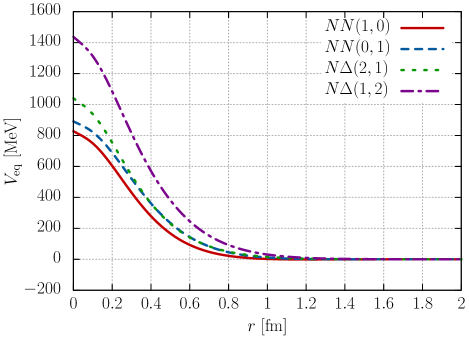
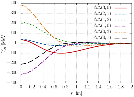
Figure 4: Equivalent local potentials for the baryon-baryon systems: strangeness $S=0$ sector.

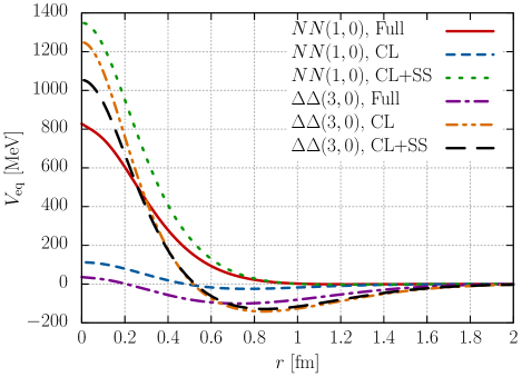
Figure 5: Decomposition of the potentials for the $NN(1,0)$ and $\Delta\Delta(3,0)$ systems.

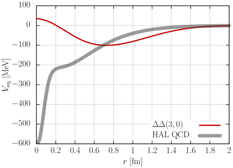
Figure 6: Comparison with the HAL QCD potential for the $\Delta\Delta(3,0)$ system Gongyo:2020pyy .

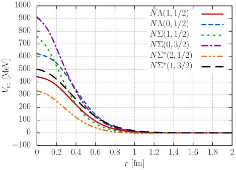
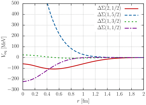
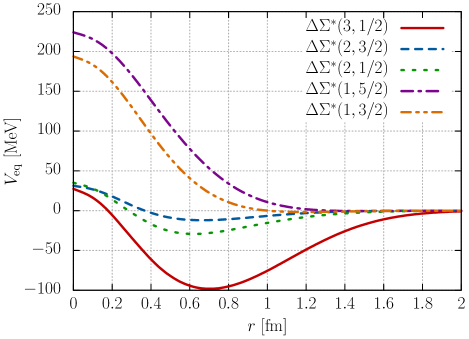
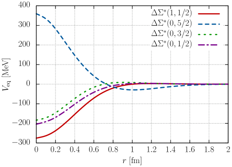
Figure 7: Equivalent local potentials for the baryon-baryon systems: strangeness $S=-1$ sector.

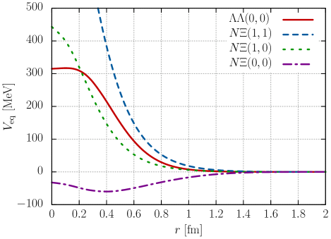
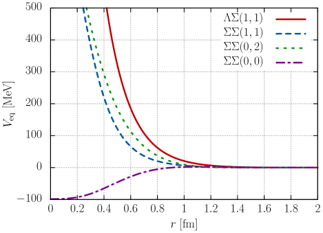
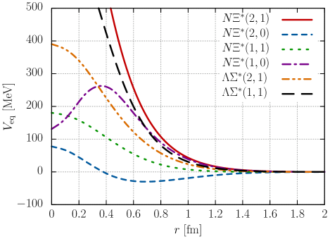
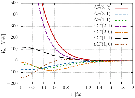
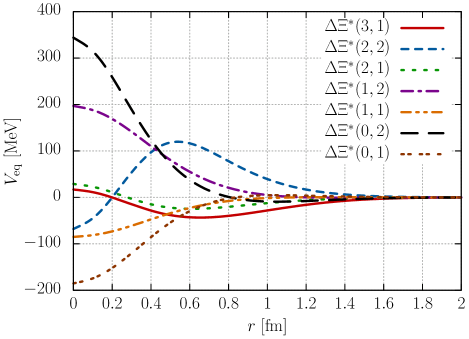
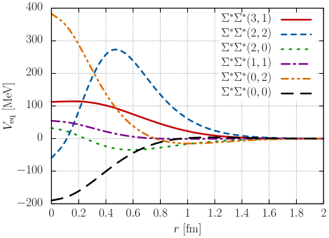
Figure 8: Equivalent local potentials for the baryon-baryon systems: strangeness $S=-2$ sector.

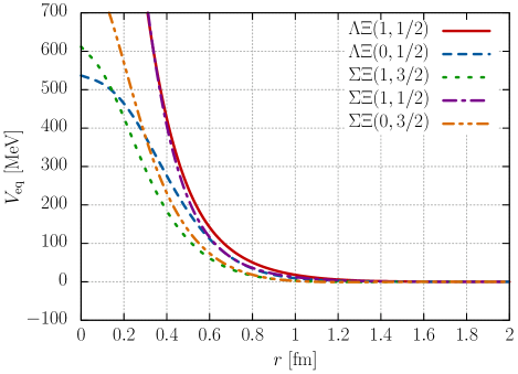
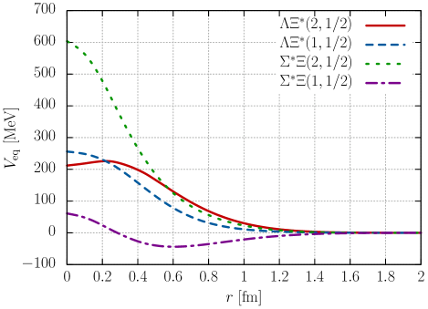
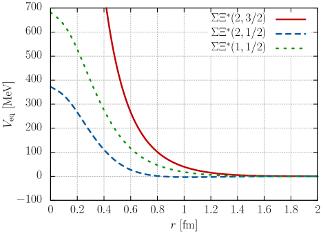
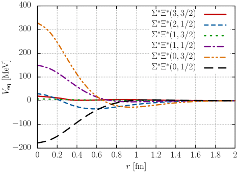
Figure 9: Equivalent local potentials for the baryon-baryon systems: strangeness $S=-3$ sector.

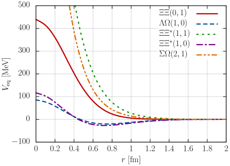
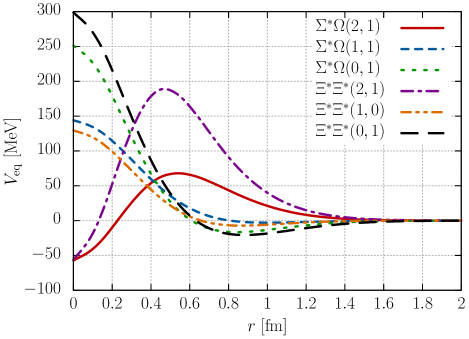
Figure 10: Equivalent local potentials for the baryon-baryon systems: strangeness $S=-4$ sector.

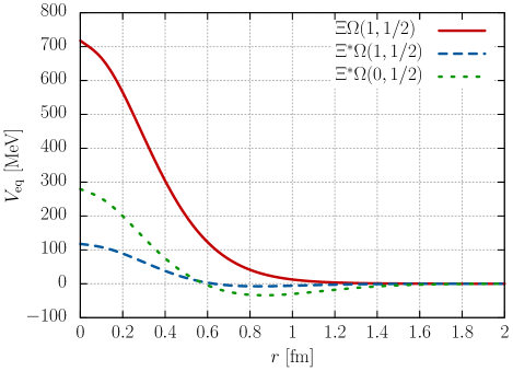
Figure 11: Equivalent local potentials for the baryon-baryon systems: strangeness $S=-5$ sector.

Figure 12: Equivalent local potentials for the baryon-baryon systems: strangeness $S=-6$ sector. We also plot the HAL QCD potential for the $\Omega\Omega(0,0)$ system Gongyo:2017fjb .

III.1 Single-channel cases

III.1.1 Two-baryon channels

Firstly, we summarize in Table 4 the two-baryon channels composed of the ground-state baryons in $S$ wave. In this study, we specify the quantum numbers of the two-baryon channels using the total spin $J$ and isospin $I$ as $(J,I)$. We perform projection onto the $(J,I)$ state using the Clebsch–Gordan coefficients in the usual manner. The same Table also lists the values of the spin-flavor [33] components for the two-baryon channels, denoted as $N_{33}$. This measures the contribution of totally antisymmetric states of six quarks for two ground-state baryons in $S$ wave. Therefore, a smaller $N_{33}$ indicates stronger repulsion due to the Pauli exclusion principle for quarks. The spin-flavor [33] component $N_{33}$ corresponds to an eigenvalue of the normalization kernel $N(\bm{r},\bm{r}^{\prime})$ associated with the eigenvector $\varphi(\bm{r})$ Oka:2000wj :

$$\int d^{3}r^{\prime}N(\bm{r},\bm{r}^{\prime})\varphi(\bm{r}^{\prime})=2N_{33}\varphi(\bm{r}).$$ (64)

We can calculate $N_{33}$ using the creation and annihilation operators of baryons. Namely, we have the formula

$$N_{33}=\frac{1}{2}\braket{B_{a}B_{b}(J,I)_{0}}{B_{a}B_{b}(J,I)_{0}},$$ (65)

where $\ket{B_{a}B_{b}(J,I)_{0}}$ is the two-baryon state with the quantum numbers $(J,I)$ but without the coordinates of quarks:

$$\ket{B_{a}B_{b}(J,I)_{0}}$$

$$\equiv\sum_{s_{a},i_{a}}\braket{J,J}{S_{a},s_{a},S_{b},J-s_{a}}\braket{I,I}{I_{a},i_{a},I_{b},I-i_{a}}$$

$$\phantom{=}\times\hat{w}^{(B_{a}(s_{a},i_{a}))\dagger}\hat{w}^{(B_{b}(J-s_{a},I-i_{a}))\dagger}\ket{0},$$ (66)

$$\hat{w}^{(B(s,i))\dagger}\equiv\sum_{\vec{\mu}}w_{\vec{\mu}}^{(B(s,i))}\hat{a}_{\mu_{1}}^{\dagger}\hat{a}_{\mu_{2}}^{\dagger}\hat{a}_{\mu_{3}}^{\dagger}.$$ (67)

Here, $S_{a}$ and $I_{a}$ are the spin and isospin values of $B_{a}$, respectively, $B(s,i)$ refers to the baryon $B$ with the third components of spin $s$ and isospin $i$, $\braket{J,j}{S_{a},s_{a},S_{b},s_{b}}$ is the Clebsch–Gordan coefficient, and the operator $\hat{a}_{\mu}^{\dagger}$ was introduced in Eq. (13). As shown in Table 4, the values of $N_{33}$ are scattered between zero and unity. In particular, when only single-channel cases are considered, the channels with $N_{33}$ close to unity usually contain decuplet baryons. We expect that these channels may avoid repulsive potentials due to the Pauli exclusion principle for quarks.

III.1.2 Strangeness $S=0$

Now, let us present the equivalent local potentials for the baryon-baryon systems with strangeness $S=0$ in Fig. 4. As seen in the figure, significant repulsive cores are observed in the potentials for the $NN(1,0)$, $NN(0,1)$, $N\Delta(2,1)$, and $N\Delta(1,2)$ systems. These cores begin to rise at approximately $1\text{\,}\mathrm{f}\mathrm{m}$. Because the spatial extension of each baryon in our model is typically less than $0.5\text{\,}\mathrm{f}\mathrm{m}$ (see Table 2), our results indicate that the interaction becomes significant when the distance between two baryons reaches the sum of their respective radii. The values of the four potentials at the origin amount to more than $800\text{\,}\mathrm{M}\mathrm{e}\mathrm{V}$, and the repulsion is strongest in the $N\Delta(1,2)$ system, followed by $N\Delta(2,1)$, $N(0,1)$, and $N(1,0)$. On the other hand, the $\Delta\Delta$ systems have moderate repulsion or even attractive cores at a short range. In particular, thanks to the attraction, the $\Delta\Delta(3,0)$ system generates a bound state, whose properties will be presented later. The behavior of these potentials is quantitatively similar to the results in Ref. Oka:1981rj . Therefore, our model with more precise wave functions strengthens the discussions in Ref. Oka:1981rj . Here, we note that the $N\Delta(2,2)$, $N\Delta(1,1)$, $\Delta\Delta(3,2)$, and $\Delta\Delta(2,3)$ systems have singular equivalent local potentials because the wave functions have nodes caused by unphysical forbidden states due to the Pauli exclusion principle for quarks. We mark these channels with a dagger ($\dagger$) in Table 4 and do not show these singular equivalent local potentials.

To confirm the mechanism of attraction/repulsion, we decompose the potentials by considering the following cases:

• Case of the color Coulomb plus linear confining force (CL): only the color Coulomb plus linear confining potential $V_{\rm CL}(r)$ is considered in the RGM equation (53), while $V_{\rm ss}(r)=0$ and $N(\bm{r},\bm{r}^{\prime})=\delta(\bm{r}-\bm{r}^{\prime})$.

• Case of the color Coulomb, linear confining, and color magnetic forces (CL+SS): both the color Coulomb plus linear confining potential $V_{\rm CL}(r)$ and the color magnetic potential $V_{\rm ss}(r)$ are considered in the RGM equation (53), while $N(\bm{r},\bm{r}^{\prime})=\delta(\bm{r}-\bm{r}^{\prime})$.

• Case of the full calculation (Full).

The resulting equivalent local potentials for the $NN(1,0)$ and $\Delta\Delta(3,0)$ systems are plotted in Fig. 5. The $NN(1,0)$ system has a moderate interaction due to the color Coulomb plus linear confining force (CL, the dashed line in Fig. 5), but when the color magnetic force is included (CL+SS, the dotted line in Fig. 5), it generates a highly repulsive potential. However, the repulsion becomes weaker when the normalization kernel $N(\bm{r},\bm{r}^{\prime})$ is considered (Full, the solid line in Fig. 5). On the other hand, the $\Delta\Delta(3,0)$ system in the CL case has an attraction in the medium range $$1\text{\,}\mathrm{f}\mathrm{m}$<r<$2\text{\,}\mathrm{f}\mathrm{m}$$ that is strong enough to produce a bound state (the double dot-dashed line in Fig. 5). This attraction grows when the color magnetic force is included (the long dashed line in Fig. 5), and the short-range repulsion becomes moderate when the normalization kernel is applied (the dot-dashed line in Fig. 5). We emphasize here that the strength of the attraction/repulsion generated by the color Coulomb plus linear confining force is correlated with the values of $N_{33}$: a larger $N_{33}$ generates stronger attraction in the CL case. Indeed, the $\Delta\Delta(0,3)$ system has the same equivalent local potential in the CL case as the $\Delta\Delta(3,0)$ system, but the repulsive color magnetic interaction in the $\Delta\Delta(0,3)$ system distorts the potential, resulting in a repulsive potential in the full calculation (the double dot-dashed line in the right panel of Fig. 4). This implies that, even if both the $\Delta\Delta(3,0)$ and $\Delta\Delta(0,3)$ dibaryon states exist as predicted in Ref. Dyson:1964xwa , their nature will be qualitatively different from each other. In summary, as discussed in Ref. Oka:1981rj , both the Pauli exclusion principle for quarks and color magnetic interactions are essential for the behavior of baryon-baryon interactions at short distances.

In Fig. 6 we compare our result for the equivalent local potential in the $\Delta\Delta(3,0)$ system with the analytic form of the HAL QCD potential with a heavy pion mass $m_{\pi}=$679\text{\,}\mathrm{M}\mathrm{e}\mathrm{V}$$ Gongyo:2020pyy . Both potentials provide sufficient attraction to generate a $\Delta\Delta(3,0)$ bound state, but the details differ. In particular, at the origin, while no repulsive core is observed in the HAL QCD potential, the potential in our quark model exhibits weak repulsion, which originates from the color Coulomb plus linear force (see Fig. 5). Such a discrepancy can be discussed, for example, by adding meson exchange contributions to our potential, as a previous study has shown that the exchanges of scalar and pseudoscalar mesons can be superposed on the quark-model potential without introducing a double-counting problem Yazaki:1989rh . In addition, the quark mass dependence of the potential in both quark models and lattice QCD simulations would be important. However, it should be noted that the potential itself is not observable and the value of the potential at the origin is not crucial for the generation of the bound state. Therefore, to evaluate the strength of the potentials, we introduce a quantity

$$\beta\equiv-\frac{16\mu_{ab}}{\pi^{2}}\int_{0}^{\infty}dr\,rV_{\rm eq}(r).$$ (68)

This quantity is motivated by the condition that a three-dimensional potential well generates a bound state. Namely, a three-dimensional potential well $V(r)=-V_{0}\theta(a-r)$, with a potential depth $V_{0}$, range $a$, and the Heaviside step function $\theta(x)$, generates a bound state if $\beta\geq 1$. The $\Delta\Delta(3,0)$ potential in our quark model provides $\beta=1.93$, while the HAL QCD potential $\beta=2.51$ with heavy $\Delta$ mass $M_{\Delta}=$1677\text{\,}\mathrm{M}\mathrm{e}\mathrm{V}$$ Gongyo:2020pyy . These values imply that the HAL QCD potential for the $\Delta\Delta(3,0)$ system with the heavy $\Delta$ mass is stronger than that in our model with the almost physical $\Delta$ mass.

III.1.3 Strangeness $S<0$

The equivalent local potentials with strangeness $S=-1$, $-2$, $-3$, $-4$, $-5$, and $-6$ are plotted in Figs. 7, 8, 9, 10, 11, and 12, respectively. We note that the $N\Omega$ and $\Delta\Omega$ interactions are absent in the single-channel cases because the shuffling of quarks associated with the quark-quark interaction inevitably leads to the transition to inelastic channels [see Fig. 3(b)]. As shown in the figures, the potentials exhibit both attractive and repulsive behavior, depending on the channels. The potentials start to deviate from zero at about $1\text{\,}\mathrm{f}\mathrm{m}$ in almost all channels, which again indicate that the interaction becomes significant when the distance between two baryons reaches the sum of their respective radii. The exception is the cases of $N_{33}\approx 1$ [for example $\Delta\Sigma^{\ast}(3,1/2)$] and $N_{33}\approx 0$ [for example $\Delta\Xi^{\ast}(2,2)$], in which the cancellation among the contributions in the color Coulomb plus linear confining forces does not occur. Consequently, the potentials become detectable even at distances with $r>$1\text{\,}\mathrm{f}\mathrm{m}$$, which corresponds to the situation that just the tails of the single-baryon wave functions start to overlap (see Fig. 2): the potentials at longer ranges exhibits negative (positive) growth in the $N_{33}\approx 1$ ($N_{33}\approx 0$) case.

In Fig. 12, we also plot the analytic form of the $\Omega\Omega(0,0)$ potential in the HAL QCD method. The behavior of the potentials in the two approaches is qualitatively consistent. The mechanism of the $\Omega\Omega(0,0)$ potential in our quark model is similar to that of the $\Delta\Delta(0,3)$: the repulsion near the origin is the sum of the contributions from the color Coulomb plus linear confining force and repulsive color magnetic force, while the medium-range attraction originates from the color Coulomb plus linear confining force. Because the strange quark is heavier than the up and down quarks, the repulsive color magnetic force, which is proportional to $1/m_{s}^{2}$ [see Eq. (32)], becomes weaker in the $\Omega\Omega(0,0)$ system, and hence the medium-range attraction persists. However, the attraction is not sufficient in our model to generate a bound state in contrast to the HAL QCD potential. Indeed, the strength of the potential $\beta$ in Eq. (68) amounts to $\beta=0.248$ ($0.937$) in our model (HAL QCD method). This discrepancy could be compensated for by including exchange forces of mesons such as the $\eta$ and $\sigma$ mesons.

III.1.4 Bound states

Table 5: Properties of the bound states.

System	$B$ [MeV]	$\sqrt{\braket{r_{\rm D}^{2}}}$ [fm]
$\Delta\Delta(3,0)$	13.1	1.70
$\Delta\Sigma(2,1/2)$	06.9	2.03
$\Delta\Sigma^{\ast}(3,1/2)$	12.6	1.68
$\Sigma\Sigma^{\ast}(2,0)$	00.7	5.24

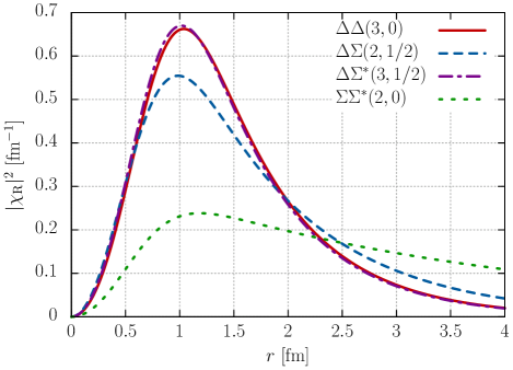
Figure 13: Square of the relative wave functions for the dibaryon bound states.

In our quark model calculations in single-channel cases, we find bound states of the $\Delta\Delta(3,0)$, $\Delta\Sigma(2,1/2)$, $\Delta\Sigma^{\ast}(3,1/2)$, and $\Sigma\Sigma^{\ast}(2,0)$ systems. Table 5 shows the binding energies $B$ and root mean squared distances between two baryons $\sqrt{\braket{r_{\rm D}^{2}}}$ of these bound states, which are defined using the normalized wave functions of the relative motion as

$$\int_{0}^{\infty}dr|\chi_{\rm R}(r)|^{2}=1,\quad\braket{r_{\rm D}^{2}}\equiv\int_{0}^{\infty}dr\,r^{2}|\chi_{\rm R}(r)|^{2}.$$ (69)

We also plot the square of the relative wave functions $|\chi_{\rm R}(r)|^{2}$ in Fig. 13. As shown by the root mean squared distances in Table 5 and the squared wave functions in Fig. 13, the spatial extension of the bound states largely exceeds the typical size of hadrons of $1\text{\,}\mathrm{f}\mathrm{m}$. This strongly suggests that these dibaryon states are hadronic molecules rather than compact hexaquark states. The $\Delta\Delta(3,0)$ bound state can be interpreted as the $d^{\ast}(2380)$ recently confirmed in experiments WASA-at-COSY:2011bjg . The $\Delta\Sigma^{\ast}(3,1/2)$ bound state was predicted in Ref. Li:2000cb in the chiral SU(3) quark model. Furthermore, the wave functions of the $\Delta\Delta(3,0)$ and $\Delta\Sigma^{\ast}(3,1/2)$ are very similar to each other. Indeed, both the normalization kernel $N(\bm{r},\bm{r}^{\prime})$ and interaction term $V_{\rm int}(\bm{r},\bm{r}^{\prime})$ are very similar in the $\Delta\Delta(3,0)$ and $\Delta\Sigma^{\ast}(3,1/2)$ systems, because they are members of the flavor antidecuplet generated by two decuplet baryons. This fact implies that bound states of the $\Delta\Xi^{\ast}$-$\Sigma^{\ast}\Sigma^{\ast}(3,1)$ and $\Delta\Omega$-$\Sigma^{\ast}\Xi^{\ast}(3,3/2)$ systems in coupled channels exist as the other members of the flavor antidecuplet, although the attraction is not sufficient in these systems in the single-channel cases. On the other hand, the $\Delta\Sigma(2,1/2)$ and $\Sigma\Sigma^{\ast}(2,0)$ systems couple to lower baryon-baryon channels $N\Sigma^{\ast}$ and $N\Xi^{\ast}$, respectively, in $S$ wave. Therefore, it is necessary to take into account the coupled-channels effects to determine the properties of these bound states.

III.2 Coupled-channels cases

In the previous subsection, we only considered the single-channel cases where transitions between inelastic channels were neglected. However, in several systems, such transitions may play a significant role. Therefore, in this subsection, we examine the coupled-channels effects.

III.2.1 Flavor antidecuplet states with $J=3$

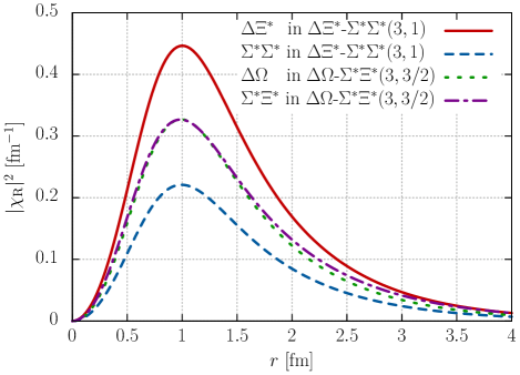
Figure 14: Square of the relative wave functions for the dibaryon bound states in coupled channels.

Firstly, we consider the coupled channels of $\Delta\Xi^{\ast}$-$\Sigma^{\ast}\Sigma^{\ast}(3,1)$ and $\Delta\Omega$-$\Sigma^{\ast}\Xi^{\ast}(3,3/2)$. They are important because they belong to the flavor antidecuplet generated by two decuplet baryons, together with the $\Delta\Delta(3,0)$ and $\Delta\Sigma^{\ast}(3,1/2)$ states, which are bound as in the previous subsection. We allow transitions between inelastic channels via $N(\bm{r},\bm{r}^{\prime})$ and $V_{\rm int}(\bm{r},\bm{r}^{\prime})$ and solve the RGM equation (53). As a result, we find bound states below the lower thresholds, i.e., the $\Sigma^{\ast}\Sigma^{\ast}$ and $\Sigma^{\ast}\Xi^{\ast}$, respectively, in our model. The $\Delta\Omega$ bound state was predicted in Ref. Li:1999bc in the chiral SU(3) quark model. In the strangeness $S=-2$ sector, the binding energy of the bound state measured from the $\Delta\Xi^{\ast}$ ($\Sigma^{\ast}\Sigma^{\ast}$) threshold is $11.7\text{\,}\mathrm{M}\mathrm{e}\mathrm{V}$ ($11.1\text{\,}\mathrm{M}\mathrm{e}\mathrm{V}$). In the strangeness $S=-3$ sector, the binding energy is $11.1\text{\,}\mathrm{M}\mathrm{e}\mathrm{V}$ ($9.0\text{\,}\mathrm{M}\mathrm{e}\mathrm{V}$) from the $\Delta\Omega$ ($\Sigma^{\ast}\Xi^{\ast}$) threshold. In Fig. 14 we plot the squared wave functions of the bound states with the normalization

$$\sum_{i}\int_{0}^{\infty}dr|\chi_{\mathrm{R},i}(r)|^{2}=1,$$ (70)

where $i$ denotes the channels. As one can see, the squared wave functions have nonzero values even above the typical size of hadrons of $1\text{\,}\mathrm{f}\mathrm{m}$, indicating that these dibaryon states are hadronic molecules rather than compact hexaquark states, as the $\Delta\Delta(3,0)$ and $\Delta\Sigma^{\ast}(3,1/2)$ bound states. Furthermore, we can evaluate the fractions of the $\Delta\Xi^{\ast}$, $\Sigma^{\ast}\Sigma^{\ast}$, $\Delta\Omega$, and $\Sigma^{\ast}\Xi^{\ast}$ components in the bound states by calculating each term of the summation in Eq. (70). The resulting fractions are $67\text{\,}\mathrm{\char 37\relax}$ ($33\text{\,}\mathrm{\char 37\relax}$) for the $\Delta\Xi^{\ast}$ ($\Sigma^{\ast}\Sigma^{\ast}$) component in the $\Delta\Xi^{\ast}$-$\Sigma^{\ast}\Sigma^{\ast}(3,1)$ bound state, and $49\text{\,}\mathrm{\char 37\relax}$ ($51\text{\,}\mathrm{\char 37\relax}$) for the $\Delta\Omega$ ($\Sigma^{\ast}\Xi^{\ast}$) component in the $\Delta\Omega$-$\Sigma^{\ast}\Xi^{\ast}(3,3/2)$ bound state. We summarize the properties of the bound states in Table 6.

Table 6: Properties of the bound and resonance states in coupled channels. In the $\Delta\Xi^{\ast}$-$\Sigma^{\ast}\Sigma^{\ast}(3,1)$ and $\Delta\Omega$-$\Sigma^{\ast}Xi^{\ast}(3,3/2)$ cases, the binding energy $B$ is measured from the $\Delta\Xi^{\ast}$ and $\Delta\Omega$ thresholds in our model, respectively. The decay width $\Gamma$ is also included in the $N\Omega(2,1/2)$ and $\Delta\Sigma(2,1/2)$ channels.

System	$B$ [MeV]	$\Gamma$ [MeV]	Note
$\Delta\Xi^{\ast}$-$\Sigma^{\ast}\Sigma^{\ast}(3,1)$	11.7	—	$\Delta\Xi^{\ast}$ $67\text{\,}\mathrm{\char 37\relax}$, $\Sigma^{\ast}\Sigma^{\ast}$ $33\text{\,}\mathrm{\char 37\relax}$
$\Delta\Omega$-$\Sigma^{\ast}\Xi^{\ast}(3,3/2)$	11.1	—	$\Delta\Omega$ $49\text{\,}\mathrm{\char 37\relax}$, $\Sigma^{\ast}\Xi^{\ast}$ $51\text{\,}\mathrm{\char 37\relax}$
$N\Omega(2,1/2)$	10.3	4.6	With meson exchanges
$\Delta\Sigma(2,1/2)$	$-40.6$	76.0	Decay to $N\Sigma^{\ast}$

Figure 15: Equivalent local potentials for the baryon-baryon systems: flavor antidecuplet states in coupled channels.

From the relative wave functions of the bound state $\chi_{\mathrm{R},i}$, we would like to extract the local coupled-channels potentials. However, in the coupled-channels cases, this task is not straightforward in contrast to the single-channel cases, because the number of coupled-channels potentials is generally larger than the number of wave equations. In particular, the wave equations in a two-channel problem become

$$\begin{pmatrix}\displaystyle-\frac{1}{2\mu_{1}}\frac{d^{2}}{dr^{2}}+V_{11}(r)&V_{12}(r)\\ V_{21}(r)&\displaystyle\Delta-\frac{1}{2\mu_{2}}\frac{d^{2}}{dr^{2}}+V_{22}(r)\end{pmatrix}\begin{pmatrix}\displaystyle\vphantom{\frac{d^{2}}{dr^{2}}}\chi_{\mathrm{R},1}\\ \displaystyle\vphantom{\frac{d^{2}}{dr^{2}}}\chi_{\mathrm{R},2}\end{pmatrix}$$

$$=-B\begin{pmatrix}\chi_{\mathrm{R},1}\\ \chi_{\mathrm{R},2}\end{pmatrix}$$ (71)

where $\Delta$ is the difference of the two threshold values and $B$ is the binding energy measured from the threshold of the first channel. We have obtained the relative wave functions $\chi_{\mathrm{R},1}$ and $\chi_{\mathrm{R},2}$ by solving the RGM equation, but they are not sufficient to uniquely determine the coupled-channels potentials $V_{11}$, $V_{12}$, $V_{21}$, and $V_{22}$. To solve this problem, we make three assumptions: 1) the potential is dominated by the antidecuplet contribution, 2) inelastic potentials are symmetric, i.e., $V_{12}=V_{21}$, and 3) the weight of each component in the antidecuplet is fixed purely by the Clebsch–Gordan coefficient. For example, in the $\Delta\Xi^{\ast}$-$\Sigma^{\ast}\Sigma^{\ast}(3,1)$ case, because the antidecuplet state $\overline{\bm{10}}$ has the relation

$$\ket{\overline{\bm{10}}(3,1)}=\sqrt{\frac{2}{3}}\ket{\Delta\Xi^{\ast}(3,1)}-\sqrt{\frac{1}{3}}\ket{\Sigma^{\ast}\Sigma^{\ast}(3,1)},$$ (72)

the equivalent local coupled-channels potentials can be evaluated by the formulae:

$$V_{\rm eq}^{\Delta\Xi^{\ast}\textrm{-}\Sigma^{\ast}\Sigma^{\ast}}(r)=V_{\rm eq}^{\Sigma^{\ast}\Sigma^{\ast}\textrm{-}\Delta\Xi^{\ast}}(r)=-\frac{1}{\sqrt{2}}V_{\rm eq}^{\Delta\Xi^{\ast}\textrm{-}\Delta\Xi^{\ast}}(r),$$ (73)

$$V_{\rm eq}^{\Delta\Xi^{\ast}\textrm{-}\Delta\Xi^{\ast}}(r)=\frac{\displaystyle\frac{1}{2\mu_{\Delta\Xi^{\ast}}}\frac{d^{2}\chi_{\mathrm{R},\Delta\Xi^{\ast}}}{dr^{2}}-B\chi_{\mathrm{R},\Delta\Xi^{\ast}}(r)}{\displaystyle\chi_{\mathrm{R},\Delta\Xi^{\ast}}(r)-\frac{1}{\sqrt{2}}\chi_{\mathrm{R},\Sigma^{\ast}\Sigma^{\ast}}(r)},$$ (74)

$$V_{\rm eq}^{\Sigma^{\ast}\Sigma^{\ast}\textrm{-}\Sigma^{\ast}\Sigma^{\ast}}(r)=\frac{1}{\chi_{\mathrm{R},\Sigma^{\ast}\Sigma^{\ast}}(r)}\left[\frac{1}{2\mu_{\Sigma^{\ast}\Sigma^{\ast}}}\frac{d^{2}\chi_{\mathrm{R},\Sigma^{\ast}\Sigma^{\ast}}}{dr^{2}}\right.$$

$$\left.\phantom{\frac{d^{2}}{dr^{2}}}-(B+\Delta)\chi_{\mathrm{R},\Sigma^{\ast}\Sigma^{\ast}}(r)-V_{\rm eq}^{\Sigma^{\ast}\Sigma^{\ast}\textrm{-}\Delta\Xi^{\ast}}(r)\chi_{\mathrm{R},\Delta\Xi^{\ast}}(r)\right].$$ (75)

We plot the calculated local coupled-channels potentials for the $\Delta\Xi^{\ast}$-$\Sigma^{\ast}\Sigma^{\ast}(3,1)$ bound state in the left panel of Fig. 15 together with the potentials in the single-channel case denoted as “single”. The elastic $\Delta\Xi^{\ast}$ potential (the solid line in the left panel of Fig. 15) becomes more attractive compared to the single-channel case (the dot-dashed line), and the elastic $\Sigma^{\ast}\Sigma^{\ast}$ potential (the dotted line) changes to attraction. Similarly, we can evaluate the equivalent local potentials for the $\Delta\Omega$-$\Sigma^{\ast}\Xi^{\ast}$ bound state via the relation

$$\ket{\overline{\bm{10}}(3,3/2)}=\frac{1}{\sqrt{2}}\ket{\Delta\Omega(3,3/2)}-\frac{1}{\sqrt{2}}\ket{\Sigma^{\ast}\Xi^{\ast}(3,3/2)}.$$ (76)

The result is plotted in the right panel of Fig. 15. Interestingly, while the $\Delta\Omega$ interaction does not occur in the single-channel case, as the quark shuffle associated with the quark-quark interaction inevitably leads to the transition to inelastic channels, the elastic $\Delta\Omega$ interaction emerges via the coupling to the $\Sigma^{\ast}\Xi^{\ast}$ and is attractive. In addition, the attraction of the elastic $\Sigma^{\ast}\Xi^{\ast}$ potential grows when the coupled channels are taken into account.

We note that, for the flavor antidecuplet $\Delta\Xi^{\ast}$-$\Sigma^{\ast}\Sigma^{\ast}(3,1)$ state with the weight in Eq. (72) and $\Delta\Omega$-$\Sigma^{\ast}\Xi^{\ast}(3,3/2)$ state with the weight in Eq. (76), the normalization kernel $N(\bm{r},\bm{r}^{\prime})$ and interaction term $V_{\rm int}(\bm{r},\bm{r}^{\prime})$ are again similar to those of the $\Delta\Delta(3,0)$ state. Therefore, we extend the discussion on the $\Delta\Delta(3,0)$ bound state and conclude that both the Pauli exclusion principle for quarks and color magnetic interactions are essential for the generation of the bound states in the flavor antidecuplet.

III.2.2 Flavor octet states with $J=2$

Next, we consider the $N\Omega(2,1/2)$ system. In the single-channel case, the $N\Omega$ interaction is absent because the shuffling of quarks associated with the quark-quark interaction inevitably leads to the transition to inelastic channels, which is the same as the $\Delta\Omega$ interaction. However, the coupled channels $\Lambda\Xi^{\ast}$, $\Sigma^{\ast}\Xi$, and $\Sigma\Xi^{\ast}$, whose thresholds are above but close to the $N\Omega$ threshold, may bring attraction to the $N\Omega(2,1/2)$ system. Indeed, the HAL QCD method has predicted a strong attraction in the $N\Omega(2,1/2)$ system HALQCD:2018qyu . As discussed in Ref. Sekihara:2018tsb , such attraction cannot be provided by conventional meson exchanges, so it is natural to examine the $N\Omega$ interaction in terms of quark degrees of freedom. Previous research on the $N\Omega$ interaction in the constituent quark model can be found in, e.g., Ref. Oka:1988yq , and we revisit this using more precise wave functions.

Figure 16: Equivalent local potential for the $N\Omega$ system in our model (solid line). We also plot the real part of the potential with the meson exchange contributions added (dashed line) and the HAL QCD potential for the $N\Omega(2,1/2)$ system HALQCD:2018qyu (thick line).

By solving the RGM equation in the coupled channels of $N\Omega$-$\Lambda\Xi^{\ast}$-$\Sigma^{\ast}\Xi$-$\Sigma\Xi^{\ast}(2,1/2)$, we find a bound state with a binding energy $B=$2.1\text{\,}\mathrm{M}\mathrm{e}\mathrm{V}$$ below the $N\Omega$ threshold. Then, assuming that the $N\Omega$ contribution is dominant near the $N\Omega$ threshold in the coupled channels, we evaluate the equivalent local potential for the elastic $N\Omega(2,1/2)$ only from the $N\Omega$ wave function at the $N\Omega$ bound state energy $\chi_{\mathrm{R},N\Omega}(r)$:

$$V_{\rm eq}^{N\Omega\textrm{-}N\Omega}(r)=-B+\frac{1}{2\mu_{N\Omega}\chi_{\mathrm{R},N\Omega}(r)}\frac{d^{2}\chi_{\mathrm{R},N\Omega}}{dr^{2}}.$$ (77)

The resulting potential is shown as the solid line in Fig. 16. This indicates that the $N\Omega(2,1/2)$ interaction is attractive via the coupled channels. The strength of the potential $\beta$ (68) is $\beta=1.29$ in our model.

Additionally, we can include the meson exchange potential calculated in Ref. Sekihara:2018tsb , in which the $\eta$ meson, correlated two mesons in the scalar-isoscalar channel, and $K$ meson in a box diagram were taken into account. As a result, we obtain a bound state with a binding energy $10.3\text{\,}\mathrm{M}\mathrm{e}\mathrm{V}$ and a decay width $4.6\text{\,}\mathrm{M}\mathrm{e}\mathrm{V}$, which arises from the decay to the $\Lambda\Xi$ and $\Sigma\Xi$ channels in $D$ wave in the box diagram. We plot the real part of the $N\Omega(2,1/2)$ potential with the meson exchange contributions added as the dashed line in Fig. 16, and also present the simulation results in the HAL QCD method HALQCD:2018qyu as the thick line. Comparing the potentials in the present study and in the HAL QCD method, the shape is different at the range $r\lesssim$0.4\text{\,}\mathrm{f}\mathrm{m}$$, which was also observed in the $\Delta\Delta(3,0)$ system in Fig. 6. Although the potential is not observable, understanding the origin of the discrepancy at the range $r\lesssim$0.4\text{\,}\mathrm{f}\mathrm{m}$$ may be important. In contrast, attraction in the longer range is similar to each other. The strength of the potential $\beta$ amounts to $\beta=1.69+0.11i$ ($\beta=1.47$) in our model (HAL QCD method).

Figure 17: Equivalent local potentials for the baryon-baryon systems: flavor octet states in coupled channels.

Similarly, we calculate the relative wave functions of the $N\Sigma^{\ast}(2,1/2)$, $N\Xi^{\ast}(2,1)$, and $N\Xi^{\ast}(2,0)$ states in the coupled-channels problems $N\Sigma^{\ast}$-$\Delta\Sigma(2,1/2)$, $N\Xi^{\ast}$-$\Lambda\Sigma^{\ast}$-$\Delta\Xi$-$\Sigma\Sigma^{\ast}(2,1)$, and $N\Xi^{\ast}$-$\Sigma\Sigma^{\ast}(2,0)$, respectively. They are of interest, because they belong to the flavor octet of the two-baryon states together with the $N\Omega$-$\Lambda\Xi^{\ast}$-$\Sigma^{\ast}\Xi$-$\Sigma\Xi^{\ast}(2,1/2)$ coupled channels Oka:1988yq , and hence we expect attractive interaction due to the coupled channels. By solving the RGM equation, we find no bound states below the $N\Sigma^{\ast}$ and $N\Xi^{\ast}$ thresholds. We calculate the equivalent local potentials for the $N\Sigma^{\ast}$ and $N\Xi^{\ast}$ systems at the $N\Sigma^{\ast}$ and $N\Xi^{\ast}$ threshold energies, respectively, and show the results in Fig. 17. As we can see, compared to the single-channel cases, the repulsion becomes moderate in the $N\Sigma^{\ast}(2,1/2)$ and $N\Xi^{\ast}(2,1)$ systems, and the attraction grows in the $N\Xi^{\ast}(2,0)$ system. To conclude whether these systems are bound or not, we have to evaluate the contributions from the meson exchanges and add them to the present potentials.

III.2.3 Bound states coupling to decay channels

Among the bound states listed in Table 5, the $\Delta\Sigma(2,1/2)$ and $\Sigma\Sigma^{\ast}(2,0)$ bound states exist above the lowest thresholds with the same quantum numbers, $N\Sigma^{\ast}$ and $N\Xi^{\ast}$, respectively. Therefore, we aim to evaluate the impact of the decay channels on these bound states by tracing the bound state poles in the complex energy plane. However, solving the fully coupled-channels RGM equation (53) for the complex eigenenergy above the lowest threshold is not feasible. To circumvent this problem, we incorporate the decay channels perturbatively. Specifically, we explicitly consider the bound-state channels, i.e., $\Delta\Sigma(2,1/2)$ and $\Sigma\Sigma^{\ast}(2,0)$, as in the single-channel cases, while implicitly accounting for the decay channels by replacing the interaction term $V_{\rm int}(\bm{r},\bm{r}^{\prime})$ with

$$V_{\rm int}(\bm{r},\bm{r}^{\prime})\to V_{\rm int}(\bm{r},\bm{r}^{\prime})+\int d^{3}r_{1}d^{3}r_{2}d^{3}r_{3}V_{\rm int}(\bm{r},\bm{r}_{1})$$

$$\times G(\mathcal{E},\bm{r}_{1},\bm{r}_{2})N^{-1}(\bm{r}_{2},\bm{r}_{3})V_{\rm int}(\bm{r}_{3},\bm{r}^{\prime})$$ (78)

where $G(\mathcal{E},\bm{r}_{1},\bm{r}_{2})$ is the loop function of the decay channel

$$G(\mathcal{E},\bm{r}_{1},\bm{r}_{2})\equiv\int\frac{d^{3}p}{(2\pi)^{3}}\frac{e^{i\bm{p}\cdot(\bm{r}_{1}-\bm{r}_{2})}}{\displaystyle\mathcal{E}+\Delta-p^{2}/(2\mu^{\prime})}$$ (79)

with $\Delta$ denoting the difference of the two threshold values and $\mu^{\prime}$ the reduced mass of the decay channel. In Eq. (78), transitions between the bound-state channel and the decay channel occur at $V_{\rm int}(\bm{r},\bm{r}_{1})$ and $N^{-1}(\bm{r}_{2},\bm{r}_{3})V_{\rm int}(\bm{r}_{3},\bm{r}^{\prime})$ of the second term.

As a result of including the decay channel, the bound state pole of the $\Sigma\Sigma^{\ast}(2,0)$ system disappears due to the repulsion from the inelastic-channel contributions, while the $\Delta\Sigma(2,1/2)$ bound state becomes a resonance with an eigenenergy of $\mathcal{E}=40.6-38.0i\,$\mathrm{M}\mathrm{e}\mathrm{V}$$, which corresponds to the binding energy $B=$-40.6\text{\,}\mathrm{M}\mathrm{e}\mathrm{V}$$ and decay width $\Gamma=$76.0\text{\,}\mathrm{M}\mathrm{e}\mathrm{V}$$. Note that the real part of the resonance pole position is above the $\Delta\Sigma$ threshold, but the pole exists in the same Riemann sheet as the bound state in the single-channel case. Therefore, if the $\Delta\Sigma(2,1/2)$ resonance exists as predicted in our calculation, it will be observed as a cusp structure at the $\Delta\Sigma$ threshold in experiments.

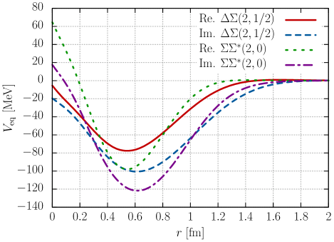
Figure 18: Equivalent local potentials for the baryon-baryon systems: inclusion of decay channels.

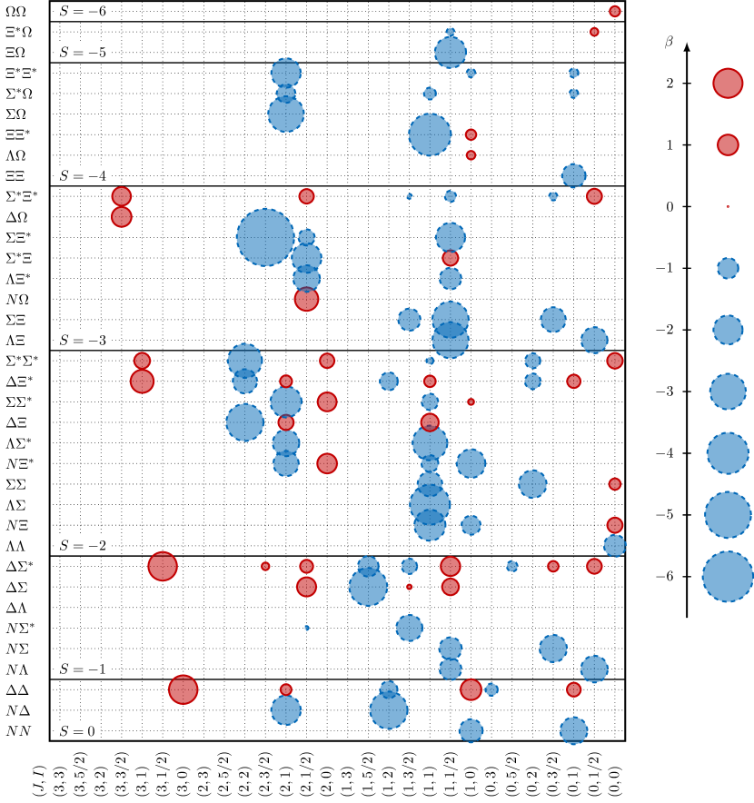
Figure 19: Strength of the potential $\beta$ (68) for the baryon-baryon systems. Red circles with solid lines represent attractive interactions, while blue circles with dashed lines represent repulsive interactions. The area of the circles corresponds to the absolute values of $\beta$.

We extract the equivalent local potential for the $\Delta\Sigma(2,1/2)$ and $\Sigma\Sigma^{\ast}(2,0)$ systems from the relative wave function $\chi_{\mathrm{R}}(r)$, where the wave function is evaluated at the threshold $\mathcal{E}=0$ for the $\Sigma\Sigma^{\ast}(2,0)$ system and at the resonance eigenenergy $\mathcal{E}=40.6-38.0i\,$\mathrm{M}\mathrm{e}\mathrm{V}$$ for the $\Delta\Sigma(2,1/2)$ system. We plot the equivalent local potentials for the $\Delta\Sigma(2,1/2)$ and $\Sigma\Sigma^{\ast}(2,0)$ systems in Fig. 18. The equivalent local potentials contain imaginary parts due to the decay channel, and the attraction of the real parts becomes moderate in both the $\Delta\Sigma(2,1/2)$ and $\Sigma\Sigma^{\ast}(2,0)$ systems. We note that, if we assume that the equivalent local potential for the $\Sigma\Sigma^{\ast}(2,0)$ in Fig. 18 is valid for any energy, the $\Sigma\Sigma^{\ast}(2,0)$ potential generates a resonance state at $\mathcal{E}=46.4-51.2i\,$\mathrm{M}\mathrm{e}\mathrm{V}$$.

III.2.4 Strength of the potentials

Finally, we calculate the strength of the potential $\beta$ (68) for all baryon-baryon systems. The results are shown in Fig. 19 as a bubble chart, where red circles with solid lines (blue circles with dashed lines) represent attractive (repulsive) interactions and the area of the circles corresponds to the absolute values of $\beta$. We use the elastic parts of the potentials for the $N\Sigma^{\ast}(2,1/2)$, $\Delta\Sigma(2,1/2)$, $N\Xi^{\ast}(2,1)$, $N\Xi^{\ast}(2,0)$, $\Sigma\Sigma^{\ast}(2,0)$, $\Delta\Xi^{\ast}(3,1)$, $\Sigma^{\ast}\Sigma^{\ast}(3,1)$, $N\Omega(2,1/2)$, $\Delta\Omega(3,3/2)$, and $\Sigma^{\ast}\Xi^{\ast}(3,3/2)$ systems in the coupled-channels cases, while using the single-channel cases for the others. We do not take meson exchange contributions into account in the $N\Omega(2,1/2)$ potential.

As shown in Fig. 19, the strongest attractions can be seen in the $\Delta\Delta(3,0)$, $\Delta\Sigma^{\ast}(3,1/2)$, $\Delta\Xi^{\ast}$-$\Sigma^{\ast}\Sigma^{\ast}(3,1)$, and $\Delta\Omega$-$\Sigma^{\ast}\Xi^{\ast}(3,3/2)$ systems, which are members of the flavor antidecuplet two-baryon states with $J=3$. The constituent quark model suggests that they are attractive enough to generate bound states. The explicit values of the strength $\beta$ are: $\beta=1.93$ for the $\Delta\Delta(3,0)$, $1.92$ for the $\Delta\Sigma^{\ast}(3,1/2)$, $1.26$ for the $\Delta\Xi^{\ast}(3,1)$, $0.594$ for the $\Sigma^{\ast}\Sigma^{\ast}(3,1)$, $0.923$ for the $\Delta\Omega(3,3/2)$, and $0.825$ for the $\Sigma^{\ast}\Xi^{\ast}(3,3/2)$ systems. Therefore, it would be interesting to perform systematic studies of the two-baryon interactions in the flavor antidecuplet states with $J=3$ in lattice QCD simulations and relativistic ion collisions as well as scattering experiments. Additionally, strong attraction $\beta>1$ can be found in the $\Delta\Delta(1,0)$ ($\beta=1.01$) and $N\Omega(2,1/2)$ ($\beta=1.29$) systems. While the $N\Omega(2,1/2)$ system generates a bound state, the attraction in the $\Delta\Delta(1,0)$ system is slightly insufficient to generate a bound state.

We would like to point out that, even if the potential is not attractive in the constituent quark model, meson exchange contributions, which are not taken into account in the present study except for the $N\Omega(2,1/2)$ system, may help in generating a bound state, as in the case of the deuteron in the $NN(1,0)$ channel. The exchanges of scalar and pseudoscalar mesons can be superposed on the quark-model potential without introducing a double-counting problem Yazaki:1989rh . In any case, the results in Fig. 19 will serve as a guideline to search for attractive interactions between two baryons and shed light on the quark dynamics inside baryons.

IV Conclusion

In this study, we investigated the short-range baryon-baryon interactions in the flavor SU(3) sector within the constituent quark model. We employed the color Coulomb, linear confining, and color magnetic forces between two constituent quarks. The wave functions of the ground-state baryons, i.e., the octet $(N,\Lambda,\Sigma,\Xi)$ and decuplet $(\Delta,\Sigma^{\ast},\Xi^{\ast},\Omega)$ baryons, were described using the Gaussian expansion method. The model parameters were determined by fitting the masses of the ground-state baryons. We used the forces between constituent quarks and baryon wave functions to systematically calculate the relative wave functions of two baryons in the resonating group method. We then evaluated the equivalent local potentials between two baryons which reproduce the relative wave functions of two baryons in the resonating group method.

The most interesting finding was the existence of two-baryon bound states with a binding energy of approximately $10\text{\,}\mathrm{M}\mathrm{e}\mathrm{V}$ in the flavor antidecuplet with total spin $J=3$, namely, $\Delta\Delta(J=3,I=0)$, $\Delta\Sigma^{\ast}(3,1/2)$, $\Delta\Xi^{\ast}$-$\Sigma^{\ast}\Sigma^{\ast}(3,1)$, and $\Delta\Omega$-$\Sigma^{\ast}\Xi^{\ast}(3,3/2)$. By decomposing the potentials for these systems, we confirmed that the contribution from the color Coulomb plus linear confining force is attractive enough to produce a bound state, and the color magnetic force brings even more attractions. We also checked that a strong attraction associated with the color Coulomb plus linear force is correlated to the spin-flavor [33] component $N_{33}$: a larger $N_{33}$ generates a stronger attraction. The spin-flavor [33] component measures the contribution of totally antisymmetric states of six quarks for two ground-state baryons in $S$ wave. In this sense, both the Pauli exclusion principle for quarks and color magnetic interactions are essential for the generation of the bound states in the flavor antidecuplet. Because the spatial extension of the bound states in the flavor antidecuplet largely exceeds the typical size of hadrons $1\text{\,}\mathrm{f}\mathrm{m}$, we concluded that these bound states are hadronic molecules rather than compact hexaquark states. In particular, the $\Delta\Delta(3,0)$ bound state can be interpreted as the $d^{\ast}(2380)$ state recently confirmed in experiments. Therefore, to understand the mechanism of the quark dynamics on the baryon-baryon interaction, the experimental search for the other members belonging to the antidecuplet will be helpful.

Another interesting finding was made in the $N\Omega(2,1/2)$ interaction. When we restrict the model space to the elastic channel, the $N\Omega$ interaction is absent in our model because the shuffling of quarks associated with the quark-quark interaction inevitably leads to a transition to inelastic channels. On the other hand, by including the coupling to inelastic channels $\Lambda\Xi^{\ast}$, $\Sigma^{\ast}\Xi$, and $\Sigma\Xi^{\ast}$, attraction in the $N\Omega(2,1/2)$ system emerges, and it is sufficient to generate a bound state with a binding energy $2.1\text{\,}\mathrm{M}\mathrm{e}\mathrm{V}$. Then, assistance comes from the meson exchange, resulting in a bound state with a binding energy $10.3\text{\,}\mathrm{M}\mathrm{e}\mathrm{V}$ and a decay width $4.6\text{\,}\mathrm{M}\mathrm{e}\mathrm{V}$. In the coupled-channels cases, we also found a resonance state $\Delta\Sigma(2,1/2)$ with the eigenenergy $\mathcal{E}=40.6-38.0i\,$\mathrm{M}\mathrm{e}\mathrm{V}$$.

The calculated equivalent local potentials between two baryons will not only be useful in further studies on dibaryon states but also provide clues to understand the mechanism of baryon-baryon interactions. When comparing the equivalent local potentials with those in the HAL QCD method for the $\Delta\Delta(3,0)$, $\Omega\Omega(0,0)$, and $N\Omega(2,1/2)$ systems, we found that, while these potentials are attractive in both approaches, their detailed shapes differ. In particular, our model provides weak repulsion at the origin in the $\Delta\Delta(3,0)$ and $N\Omega(2,1/2)$ systems, in contrast to the HAL QCD potentials. In the $\Delta\Delta(3,0)$ system, this weak repulsion at the origin comes from the color Coulomb plus linear confining force. Although the potential is not observable, understanding the origin of the discrepancy at short distances may be important. Besides, the $\Omega\Omega(0,0)$ potential in our model is weaker and not sufficiently attractive to generate a bound state, which implies that meson exchange contributions may assist the attraction. We also evaluated the strength of the potentials, which will be a guideline to search for the attractive interactions between two baryons and shed light on the quark dynamics inside baryons.

Appendix A Weights for baryons

We summarize the weights $w_{\vec{\mu}}$ for the ground-state baryons in Table 7.

Table 7: Weights for the octet and decuplet baryons. The index $s$ is the third component of the spin. “RGB cyclic” means that the terms of color permutation $(\mathrm{R},\mathrm{G},\mathrm{B})\to(\mathrm{G},\mathrm{B},\mathrm{R})$, $(\mathrm{B},\mathrm{R},\mathrm{G})$ follow with the same weight, flavor, and spin.

Octet baryons $p(s=1/2)$ $w_{\vec{\mu}}$ $\mu_{1}$ $\mu_{2}$ $\mu_{3}$ $2/3\sqrt{2}$ $(u,\uparrow,\mathrm{R})$ $(u,\uparrow,\mathrm{G})$ $(d,\downarrow,\mathrm{B})$ $-1/3\sqrt{2}$ $(u,\uparrow,\mathrm{R})$ $(u,\downarrow,\mathrm{G})$ $(d,\uparrow,\mathrm{B})$ $-1/3\sqrt{2}$ $(u,\downarrow,\mathrm{R})$ $(u,\uparrow,\mathrm{G})$ $(d,\uparrow,\mathrm{B})$ RGB cyclic $p(s=-1/2)$ $w_{\vec{\mu}}$ $\mu_{1}$ $\mu_{2}$ $\mu_{3}$ $-2/3\sqrt{2}$ $(u,\downarrow,\mathrm{R})$ $(u,\downarrow,\mathrm{G})$ $(d,\uparrow,\mathrm{B})$ $1/3\sqrt{2}$ $(u,\uparrow,\mathrm{R})$ $(u,\downarrow,\mathrm{G})$ $(d,\downarrow,\mathrm{B})$ $1/3\sqrt{2}$ $(u,\downarrow,\mathrm{R})$ $(u,\uparrow,\mathrm{G})$ $(d,\downarrow,\mathrm{B})$ RGB cyclic $n(s=1/2)$ $w_{\vec{\mu}}$ $\mu_{1}$ $\mu_{2}$ $\mu_{3}$ $-2/3\sqrt{2}$ $(d,\uparrow,\mathrm{R})$ $(d,\uparrow,\mathrm{G})$ $(u,\downarrow,\mathrm{B})$ $1/3\sqrt{2}$ $(d,\uparrow,\mathrm{R})$ $(d,\downarrow,\mathrm{G})$ $(u,\uparrow,\mathrm{B})$ $1/3\sqrt{2}$ $(d,\downarrow,\mathrm{R})$ $(d,\uparrow,\mathrm{G})$ $(u,\uparrow,\mathrm{B})$ RGB cyclic $n(s=-1/2)$ $w_{\vec{\mu}}$ $\mu_{1}$ $\mu_{2}$ $\mu_{3}$ $2/3\sqrt{2}$ $(d,\downarrow,\mathrm{R})$ $(d,\downarrow,\mathrm{G})$ $(u,\uparrow,\mathrm{B})$ $-1/3\sqrt{2}$ $(d,\uparrow,\mathrm{R})$ $(d,\downarrow,\mathrm{G})$ $(u,\downarrow,\mathrm{B})$ $-1/3\sqrt{2}$ $(d,\downarrow,\mathrm{R})$ $(d,\uparrow,\mathrm{G})$ $(u,\downarrow,\mathrm{B})$ RGB cyclic $\Lambda(s=1/2)$ $w_{\vec{\mu}}$ $\mu_{1}$ $\mu_{2}$ $\mu_{3}$ $1/2\sqrt{3}$ $(u,\uparrow,\mathrm{R})$ $(d,\downarrow,\mathrm{G})$ $(s,\uparrow,\mathrm{B})$ $-1/2\sqrt{3}$ $(u,\downarrow,\mathrm{R})$ $(d,\uparrow,\mathrm{G})$ $(s,\uparrow,\mathrm{B})$ $-1/2\sqrt{3}$ $(u,\uparrow,\mathrm{G})$ $(d,\downarrow,\mathrm{R})$ $(s,\uparrow,\mathrm{B})$ $1/2\sqrt{3}$ $(u,\downarrow,\mathrm{G})$ $(d,\uparrow,\mathrm{R})$ $(s,\uparrow,\mathrm{B})$ RGB cyclic $\Lambda(s=-1/2)$ $w_{\vec{\mu}}$ $\mu_{1}$ $\mu_{2}$ $\mu_{3}$ $1/2\sqrt{3}$ $(u,\uparrow,\mathrm{R})$ $(d,\downarrow,\mathrm{G})$ $(s,\downarrow,\mathrm{B})$ $-1/2\sqrt{3}$ $(u,\downarrow,\mathrm{R})$ $(d,\uparrow,\mathrm{G})$ $(s,\downarrow,\mathrm{B})$ $-1/2\sqrt{3}$ $(u,\uparrow,\mathrm{G})$ $(d,\downarrow,\mathrm{R})$ $(s,\downarrow,\mathrm{B})$ $1/2\sqrt{3}$ $(u,\downarrow,\mathrm{G})$ $(d,\uparrow,\mathrm{R})$ $(s,\downarrow,\mathrm{B})$ RGB cyclic

$\Sigma^{+}(s=1/2)$ $w_{\vec{\mu}}$ $\mu_{1}$ $\mu_{2}$ $\mu_{3}$ $2/3\sqrt{2}$ $(u,\uparrow,\mathrm{R})$ $(u,\uparrow,\mathrm{G})$ $(s,\downarrow,\mathrm{B})$ $-1/3\sqrt{2}$ $(u,\uparrow,\mathrm{R})$ $(u,\downarrow,\mathrm{G})$ $(s,\uparrow,\mathrm{B})$ $-1/3\sqrt{2}$ $(u,\downarrow,\mathrm{R})$ $(u,\uparrow,\mathrm{G})$ $(s,\uparrow,\mathrm{B})$ RGB cyclic $\Sigma^{+}(s=-1/2)$ $w_{\vec{\mu}}$ $\mu_{1}$ $\mu_{2}$ $\mu_{3}$ $-2/3\sqrt{2}$ $(u,\downarrow,\mathrm{R})$ $(u,\downarrow,\mathrm{G})$ $(s,\uparrow,\mathrm{B})$ $1/3\sqrt{2}$ $(u,\uparrow,\mathrm{R})$ $(u,\downarrow,\mathrm{G})$ $(s,\downarrow,\mathrm{B})$ $1/3\sqrt{2}$ $(u,\downarrow,\mathrm{R})$ $(u,\uparrow,\mathrm{G})$ $(s,\downarrow,\mathrm{B})$ RGB cyclic $\Sigma^{0}(s=1/2)$ $w_{\vec{\mu}}$ $\mu_{1}$ $\mu_{2}$ $\mu_{3}$ $1/3$ $(u,\uparrow,\mathrm{R})$ $(d,\uparrow,\mathrm{G})$ $(s,\downarrow,\mathrm{B})$ $-1/6$ $(u,\uparrow,\mathrm{R})$ $(d,\downarrow,\mathrm{G})$ $(s,\uparrow,\mathrm{B})$ $-1/6$ $(u,\downarrow,\mathrm{R})$ $(d,\uparrow,\mathrm{G})$ $(s,\uparrow,\mathrm{B})$ $-1/3$ $(u,\uparrow,\mathrm{G})$ $(d,\uparrow,\mathrm{R})$ $(s,\downarrow,\mathrm{B})$ $1/6$ $(u,\uparrow,\mathrm{G})$ $(d,\downarrow,\mathrm{R})$ $(s,\uparrow,\mathrm{B})$ $1/6$ $(u,\downarrow,\mathrm{G})$ $(d,\uparrow,\mathrm{R})$ $(s,\uparrow,\mathrm{B})$ RGB cyclic $\Sigma^{0}(s=-1/2)$ $w_{\vec{\mu}}$ $\mu_{1}$ $\mu_{2}$ $\mu_{3}$ $-1/3$ $(u,\downarrow,\mathrm{R})$ $(d,\downarrow,\mathrm{G})$ $(s,\uparrow,\mathrm{B})$ $1/6$ $(u,\uparrow,\mathrm{R})$ $(d,\downarrow,\mathrm{G})$ $(s,\downarrow,\mathrm{B})$ $1/6$ $(u,\downarrow,\mathrm{R})$ $(d,\uparrow,\mathrm{G})$ $(s,\downarrow,\mathrm{B})$ $1/3$ $(u,\downarrow,\mathrm{G})$ $(d,\downarrow,\mathrm{R})$ $(s,\uparrow,\mathrm{B})$ $-1/6$ $(u,\uparrow,\mathrm{G})$ $(d,\downarrow,\mathrm{R})$ $(s,\downarrow,\mathrm{B})$ $-1/6$ $(u,\downarrow,\mathrm{G})$ $(d,\uparrow,\mathrm{R})$ $(s,\downarrow,\mathrm{B})$ RGB cyclic

$\Sigma^{-}(s=1/2)$ $w_{\vec{\mu}}$ $\mu_{1}$ $\mu_{2}$ $\mu_{3}$ $2/3\sqrt{2}$ $(d,\uparrow,\mathrm{R})$ $(d,\uparrow,\mathrm{G})$ $(s,\downarrow,\mathrm{B})$ $-1/3\sqrt{2}$ $(d,\uparrow,\mathrm{R})$ $(d,\downarrow,\mathrm{G})$ $(s,\uparrow,\mathrm{B})$ $-1/3\sqrt{2}$ $(d,\downarrow,\mathrm{R})$ $(d,\uparrow,\mathrm{G})$ $(s,\uparrow,\mathrm{B})$ RGB cyclic $\Sigma^{-}(s=-1/2)$ $w_{\vec{\mu}}$ $\mu_{1}$ $\mu_{2}$ $\mu_{3}$ $-2/3\sqrt{2}$ $(d,\downarrow,\mathrm{R})$ $(d,\downarrow,\mathrm{G})$ $(s,\uparrow,\mathrm{B})$ $1/3\sqrt{2}$ $(d,\uparrow,\mathrm{R})$ $(d,\downarrow,\mathrm{G})$ $(s,\downarrow,\mathrm{B})$ $1/3\sqrt{2}$ $(d,\downarrow,\mathrm{R})$ $(d,\uparrow,\mathrm{G})$ $(s,\downarrow,\mathrm{B})$ RGB cyclic $\Xi^{0}(s=1/2)$ $w_{\vec{\mu}}$ $\mu_{1}$ $\mu_{2}$ $\mu_{3}$ $-2/3\sqrt{2}$ $(u,\downarrow,\mathrm{R})$ $(s,\uparrow,\mathrm{G})$ $(s,\uparrow,\mathrm{B})$ $1/3\sqrt{2}$ $(u,\uparrow,\mathrm{R})$ $(s,\uparrow,\mathrm{G})$ $(s,\downarrow,\mathrm{B})$ $1/3\sqrt{2}$ $(u,\uparrow,\mathrm{R})$ $(s,\downarrow,\mathrm{G})$ $(s,\uparrow,\mathrm{B})$ RGB cyclic $\Xi^{0}(s=-1/2)$ $w_{\vec{\mu}}$ $\mu_{1}$ $\mu_{2}$ $\mu_{3}$ $2/3\sqrt{2}$ $(u,\uparrow,\mathrm{R})$ $(s,\downarrow,\mathrm{G})$ $(s,\downarrow,\mathrm{B})$ $-1/3\sqrt{2}$ $(u,\downarrow,\mathrm{R})$ $(s,\uparrow,\mathrm{G})$ $(s,\downarrow,\mathrm{B})$ $-1/3\sqrt{2}$ $(u,\downarrow,\mathrm{R})$ $(s,\downarrow,\mathrm{G})$ $(s,\uparrow,\mathrm{B})$ RGB cyclic $\Xi^{-}(s=1/2)$ $w_{\vec{\mu}}$ $\mu_{1}$ $\mu_{2}$ $\mu_{3}$ $-2/3\sqrt{2}$ $(d,\downarrow,\mathrm{R})$ $(s,\uparrow,\mathrm{G})$ $(s,\uparrow,\mathrm{B})$ $1/3\sqrt{2}$ $(d,\uparrow,\mathrm{R})$ $(s,\uparrow,\mathrm{G})$ $(s,\downarrow,\mathrm{B})$ $1/3\sqrt{2}$ $(d,\uparrow,\mathrm{R})$ $(s,\downarrow,\mathrm{G})$ $(s,\uparrow,\mathrm{B})$ RGB cyclic $\Xi^{-}(s=-1/2)$ $w_{\vec{\mu}}$ $\mu_{1}$ $\mu_{2}$ $\mu_{3}$ $2/3\sqrt{2}$ $(d,\uparrow,\mathrm{R})$ $(s,\downarrow,\mathrm{G})$ $(s,\downarrow,\mathrm{B})$ $-1/3\sqrt{2}$ $(d,\downarrow,\mathrm{R})$ $(s,\uparrow,\mathrm{G})$ $(s,\downarrow,\mathrm{B})$ $-1/3\sqrt{2}$ $(d,\downarrow,\mathrm{R})$ $(s,\downarrow,\mathrm{G})$ $(s,\uparrow,\mathrm{B})$ RGB cyclic

Table 7: (continued)

Decuplet baryons $\Delta^{++}(s=3/2)$ $w_{\vec{\mu}}$ $\mu_{1}$ $\mu_{2}$ $\mu_{3}$ $1$ $(u,\uparrow,\mathrm{R})$ $(u,\uparrow,\mathrm{G})$ $(u,\uparrow,\mathrm{B})$ $\Delta^{++}(s=1/2)$ $w_{\vec{\mu}}$ $\mu_{1}$ $\mu_{2}$ $\mu_{3}$ $1/\sqrt{3}$ $(u,\uparrow,\mathrm{R})$ $(u,\uparrow,\mathrm{G})$ $(u,\downarrow,\mathrm{B})$ RGB cyclic $\Delta^{++}(s=-1/2)$ $w_{\vec{\mu}}$ $\mu_{1}$ $\mu_{2}$ $\mu_{3}$ $1/\sqrt{3}$ $(u,\uparrow,\mathrm{R})$ $(u,\downarrow,\mathrm{G})$ $(u,\downarrow,\mathrm{B})$ RGB cyclic $\Delta^{++}(s=-3/2)$ $w_{\vec{\mu}}$ $\mu_{1}$ $\mu_{2}$ $\mu_{3}$ $1$ $(u,\downarrow,\mathrm{R})$ $(u,\downarrow,\mathrm{G})$ $(u,\downarrow,\mathrm{B})$ $\Delta^{+}(s=3/2)$ $w_{\vec{\mu}}$ $\mu_{1}$ $\mu_{2}$ $\mu_{3}$ $1/\sqrt{3}$ $(u,\uparrow,\mathrm{R})$ $(u,\uparrow,\mathrm{G})$ $(d,\uparrow,\mathrm{B})$ RGB cyclic $\Delta^{+}(s=1/2)$ $w_{\vec{\mu}}$ $\mu_{1}$ $\mu_{2}$ $\mu_{3}$ $1/3$ $(u,\uparrow,\mathrm{R})$ $(u,\uparrow,\mathrm{G})$ $(d,\downarrow,\mathrm{B})$ $1/3$ $(u,\uparrow,\mathrm{R})$ $(u,\downarrow,\mathrm{G})$ $(d,\uparrow,\mathrm{B})$ $1/3$ $(u,\downarrow,\mathrm{R})$ $(u,\uparrow,\mathrm{G})$ $(d,\uparrow,\mathrm{B})$ RGB cyclic $\Delta^{+}(s=-1/2)$ $w_{\vec{\mu}}$ $\mu_{1}$ $\mu_{2}$ $\mu_{3}$ $1/3$ $(u,\uparrow,\mathrm{R})$ $(u,\downarrow,\mathrm{G})$ $(d,\downarrow,\mathrm{B})$ $1/3$ $(u,\downarrow,\mathrm{R})$ $(u,\uparrow,\mathrm{G})$ $(d,\downarrow,\mathrm{B})$ $1/3$ $(u,\downarrow,\mathrm{R})$ $(u,\downarrow,\mathrm{G})$ $(d,\uparrow,\mathrm{B})$ RGB cyclic $\Delta^{+}(s=-3/2)$ $w_{\vec{\mu}}$ $\mu_{1}$ $\mu_{2}$ $\mu_{3}$ $1/\sqrt{3}$ $(u,\downarrow,\mathrm{R})$ $(u,\downarrow,\mathrm{G})$ $(d,\downarrow,\mathrm{B})$ RGB cyclic $\Delta^{0}(s=3/2)$ $w_{\vec{\mu}}$ $\mu_{1}$ $\mu_{2}$ $\mu_{3}$ $1/\sqrt{3}$ $(u,\uparrow,\mathrm{R})$ $(d,\uparrow,\mathrm{G})$ $(d,\uparrow,\mathrm{B})$ RGB cyclic $\Delta^{0}(s=1/2)$ $w_{\vec{\mu}}$ $\mu_{1}$ $\mu_{2}$ $\mu_{3}$ $1/3$ $(u,\uparrow,\mathrm{R})$ $(d,\uparrow,\mathrm{G})$ $(d,\downarrow,\mathrm{B})$ $1/3$ $(u,\uparrow,\mathrm{R})$ $(d,\downarrow,\mathrm{G})$ $(d,\uparrow,\mathrm{B})$ $1/3$ $(u,\downarrow,\mathrm{R})$ $(d,\uparrow,\mathrm{G})$ $(d,\uparrow,\mathrm{B})$ RGB cyclic

$\Delta^{0}(s=-1/2)$ $w_{\vec{\mu}}$ $\mu_{1}$ $\mu_{2}$ $\mu_{3}$ $1/3$ $(u,\uparrow,\mathrm{R})$ $(d,\downarrow,\mathrm{G})$ $(d,\downarrow,\mathrm{B})$ $1/3$ $(u,\downarrow,\mathrm{R})$ $(d,\uparrow,\mathrm{G})$ $(d,\downarrow,\mathrm{B})$ $1/3$ $(u,\downarrow,\mathrm{R})$ $(d,\downarrow,\mathrm{G})$ $(d,\uparrow,\mathrm{B})$ RGB cyclic $\Delta^{0}(s=-3/2)$ $w_{\vec{\mu}}$ $\mu_{1}$ $\mu_{2}$ $\mu_{3}$ $1/\sqrt{3}$ $(u,\downarrow,\mathrm{R})$ $(d,\downarrow,\mathrm{G})$ $(d,\downarrow,\mathrm{B})$ RGB cyclic $\Delta^{-}(s=3/2)$ $w_{\vec{\mu}}$ $\mu_{1}$ $\mu_{2}$ $\mu_{3}$ $1$ $(d,\uparrow,\mathrm{R})$ $(d,\uparrow,\mathrm{G})$ $(d,\uparrow,\mathrm{B})$ $\Delta^{-}(s=1/2)$ $w_{\vec{\mu}}$ $\mu_{1}$ $\mu_{2}$ $\mu_{3}$ $1/\sqrt{3}$ $(d,\uparrow,\mathrm{R})$ $(d,\uparrow,\mathrm{G})$ $(d,\downarrow,\mathrm{B})$ RGB cyclic $\Delta^{-}(s=-1/2)$ $w_{\vec{\mu}}$ $\mu_{1}$ $\mu_{2}$ $\mu_{3}$ $1/\sqrt{3}$ $(d,\uparrow,\mathrm{R})$ $(d,\downarrow,\mathrm{G})$ $(d,\downarrow,\mathrm{B})$ RGB cyclic $\Delta^{-}(s=-3/2)$ $w_{\vec{\mu}}$ $\mu_{1}$ $\mu_{2}$ $\mu_{3}$ $1$ $(d,\downarrow,\mathrm{R})$ $(d,\downarrow,\mathrm{G})$ $(d,\downarrow,\mathrm{B})$ $\Sigma^{\ast+}(s=3/2)$ $w_{\vec{\mu}}$ $\mu_{1}$ $\mu_{2}$ $\mu_{3}$ $1/\sqrt{3}$ $(u,\uparrow,\mathrm{R})$ $(u,\uparrow,\mathrm{G})$ $(s,\uparrow,\mathrm{B})$ RGB cyclic $\Sigma^{\ast+}(s=1/2)$ $w_{\vec{\mu}}$ $\mu_{1}$ $\mu_{2}$ $\mu_{3}$ $1/3$ $(u,\uparrow,\mathrm{R})$ $(u,\uparrow,\mathrm{G})$ $(s,\downarrow,\mathrm{B})$ $1/3$ $(u,\uparrow,\mathrm{R})$ $(u,\downarrow,\mathrm{G})$ $(s,\uparrow,\mathrm{B})$ $1/3$ $(u,\downarrow,\mathrm{R})$ $(u,\uparrow,\mathrm{G})$ $(s,\uparrow,\mathrm{B})$ RGB cyclic $\Sigma^{\ast+}(s=-1/2)$ $w_{\vec{\mu}}$ $\mu_{1}$ $\mu_{2}$ $\mu_{3}$ $1/3$ $(u,\uparrow,\mathrm{R})$ $(u,\downarrow,\mathrm{G})$ $(s,\downarrow,\mathrm{B})$ $1/3$ $(u,\downarrow,\mathrm{R})$ $(u,\uparrow,\mathrm{G})$ $(s,\downarrow,\mathrm{B})$ $1/3$ $(u,\downarrow,\mathrm{R})$ $(u,\downarrow,\mathrm{G})$ $(s,\uparrow,\mathrm{B})$ RGB cyclic $\Sigma^{\ast+}(s=-3/2)$ $w_{\vec{\mu}}$ $\mu_{1}$ $\mu_{2}$ $\mu_{3}$ $1/\sqrt{3}$ $(u,\downarrow,\mathrm{R})$ $(u,\downarrow,\mathrm{G})$ $(s,\downarrow,\mathrm{B})$ RGB cyclic

$\Sigma^{\ast 0}(s=3/2)$ $w_{\vec{\mu}}$ $\mu_{1}$ $\mu_{2}$ $\mu_{3}$ $1/\sqrt{6}$ $(u,\uparrow,\mathrm{R})$ $(d,\uparrow,\mathrm{G})$ $(s,\uparrow,\mathrm{B})$ $-1/\sqrt{6}$ $(u,\uparrow,\mathrm{G})$ $(d,\uparrow,\mathrm{R})$ $(s,\uparrow,\mathrm{B})$ RGB cyclic $\Sigma^{\ast 0}(s=1/2)$ $w_{\vec{\mu}}$ $\mu_{1}$ $\mu_{2}$ $\mu_{3}$ $1/3\sqrt{2}$ $(u,\uparrow,\mathrm{R})$ $(d,\uparrow,\mathrm{G})$ $(s,\downarrow,\mathrm{B})$ $1/3\sqrt{2}$ $(u,\uparrow,\mathrm{R})$ $(d,\downarrow,\mathrm{G})$ $(s,\uparrow,\mathrm{B})$ $1/3\sqrt{2}$ $(u,\downarrow,\mathrm{R})$ $(d,\uparrow,\mathrm{G})$ $(s,\uparrow,\mathrm{B})$ $-1/3\sqrt{2}$ $(u,\uparrow,\mathrm{G})$ $(d,\uparrow,\mathrm{R})$ $(s,\downarrow,\mathrm{B})$ $-1/3\sqrt{2}$ $(u,\uparrow,\mathrm{G})$ $(d,\downarrow,\mathrm{R})$ $(s,\uparrow,\mathrm{B})$ $-1/3\sqrt{2}$ $(u,\downarrow,\mathrm{G})$ $(d,\uparrow,\mathrm{R})$ $(s,\uparrow,\mathrm{B})$ RGB cyclic $\Sigma^{\ast 0}(s=-1/2)$ $w_{\vec{\mu}}$ $\mu_{1}$ $\mu_{2}$ $\mu_{3}$ $1/3\sqrt{2}$ $(u,\uparrow,\mathrm{R})$ $(d,\downarrow,\mathrm{G})$ $(s,\downarrow,\mathrm{B})$ $1/3\sqrt{2}$ $(u,\downarrow,\mathrm{R})$ $(d,\uparrow,\mathrm{G})$ $(s,\downarrow,\mathrm{B})$ $1/3\sqrt{2}$ $(u,\downarrow,\mathrm{R})$ $(d,\downarrow,\mathrm{G})$ $(s,\uparrow,\mathrm{B})$ $-1/3\sqrt{2}$ $(u,\uparrow,\mathrm{G})$ $(d,\downarrow,\mathrm{R})$ $(s,\downarrow,\mathrm{B})$ $-1/3\sqrt{2}$ $(u,\downarrow,\mathrm{G})$ $(d,\uparrow,\mathrm{R})$ $(s,\downarrow,\mathrm{B})$ $-1/3\sqrt{2}$ $(u,\downarrow,\mathrm{G})$ $(d,\downarrow,\mathrm{R})$ $(s,\uparrow,\mathrm{B})$ RGB cyclic $\Sigma^{\ast 0}(s=-3/2)$ $w_{\vec{\mu}}$ $\mu_{1}$ $\mu_{2}$ $\mu_{3}$ $1/\sqrt{6}$ $(u,\downarrow,\mathrm{R})$ $(d,\downarrow,\mathrm{G})$ $(s,\downarrow,\mathrm{B})$ $-1/\sqrt{6}$ $(u,\downarrow,\mathrm{G})$ $(d,\downarrow,\mathrm{R})$ $(s,\downarrow,\mathrm{B})$ RGB cyclic $\Sigma^{\ast-}(s=3/2)$ $w_{\vec{\mu}}$ $\mu_{1}$ $\mu_{2}$ $\mu_{3}$ $1/\sqrt{3}$ $(d,\uparrow,\mathrm{R})$ $(d,\uparrow,\mathrm{G})$ $(s,\uparrow,\mathrm{B})$ RGB cyclic $\Sigma^{\ast-}(s=1/2)$ $w_{\vec{\mu}}$ $\mu_{1}$ $\mu_{2}$ $\mu_{3}$ $1/3$ $(d,\uparrow,\mathrm{R})$ $(d,\uparrow,\mathrm{G})$ $(s,\downarrow,\mathrm{B})$ $1/3$ $(d,\uparrow,\mathrm{R})$ $(d,\downarrow,\mathrm{G})$ $(s,\uparrow,\mathrm{B})$ $1/3$ $(d,\downarrow,\mathrm{R})$ $(d,\uparrow,\mathrm{G})$ $(s,\uparrow,\mathrm{B})$ RGB cyclic $\Sigma^{\ast-}(s=-1/2)$ $w_{\vec{\mu}}$ $\mu_{1}$ $\mu_{2}$ $\mu_{3}$ $1/3$ $(d,\uparrow,\mathrm{R})$ $(d,\downarrow,\mathrm{G})$ $(s,\downarrow,\mathrm{B})$ $1/3$ $(d,\downarrow,\mathrm{R})$ $(d,\uparrow,\mathrm{G})$ $(s,\downarrow,\mathrm{B})$ $1/3$ $(d,\downarrow,\mathrm{R})$ $(d,\downarrow,\mathrm{G})$ $(s,\uparrow,\mathrm{B})$ RGB cyclic $\Sigma^{\ast-}(s=-3/2)$ $w_{\vec{\mu}}$ $\mu_{1}$ $\mu_{2}$ $\mu_{3}$ $1/\sqrt{3}$ $(d,\downarrow,\mathrm{R})$ $(d,\downarrow,\mathrm{G})$ $(s,\downarrow,\mathrm{B})$ RGB cyclic

Table 7: (continued)

$\Xi^{\ast 0}(s=3/2)$ $w_{\vec{\mu}}$ $\mu_{1}$ $\mu_{2}$ $\mu_{3}$ $1/\sqrt{3}$ $(u,\uparrow,\mathrm{R})$ $(s,\uparrow,\mathrm{G})$ $(s,\uparrow,\mathrm{B})$ RGB cyclic $\Xi^{\ast 0}(s=1/2)$ $w_{\vec{\mu}}$ $\mu_{1}$ $\mu_{2}$ $\mu_{3}$ $1/3$ $(u,\uparrow,\mathrm{R})$ $(s,\uparrow,\mathrm{G})$ $(s,\downarrow,\mathrm{B})$ $1/3$ $(u,\uparrow,\mathrm{R})$ $(s,\downarrow,\mathrm{G})$ $(s,\uparrow,\mathrm{B})$ $1/3$ $(u,\downarrow,\mathrm{R})$ $(s,\uparrow,\mathrm{G})$ $(s,\uparrow,\mathrm{B})$ RGB cyclic $\Xi^{\ast 0}(s=-1/2)$ $w_{\vec{\mu}}$ $\mu_{1}$ $\mu_{2}$ $\mu_{3}$ $1/3$ $(u,\uparrow,\mathrm{R})$ $(s,\downarrow,\mathrm{G})$ $(s,\downarrow,\mathrm{B})$ $1/3$ $(u,\downarrow,\mathrm{R})$ $(s,\uparrow,\mathrm{G})$ $(s,\downarrow,\mathrm{B})$ $1/3$ $(u,\downarrow,\mathrm{R})$ $(s,\downarrow,\mathrm{G})$ $(s,\uparrow,\mathrm{B})$ RGB cyclic $\Xi^{\ast 0}(s=-3/2)$ $w_{\vec{\mu}}$ $\mu_{1}$ $\mu_{2}$ $\mu_{3}$ $1/\sqrt{3}$ $(u,\downarrow,\mathrm{R})$ $(s,\downarrow,\mathrm{G})$ $(s,\downarrow,\mathrm{B})$ RGB cyclic

$\Xi^{\ast-}(s=3/2)$ $w_{\vec{\mu}}$ $\mu_{1}$ $\mu_{2}$ $\mu_{3}$ $1/\sqrt{3}$ $(d,\uparrow,\mathrm{R})$ $(s,\uparrow,\mathrm{G})$ $(s,\uparrow,\mathrm{B})$ RGB cyclic $\Xi^{\ast-}(s=1/2)$ $w_{\vec{\mu}}$ $\mu_{1}$ $\mu_{2}$ $\mu_{3}$ $1/3$ $(d,\uparrow,\mathrm{R})$ $(s,\uparrow,\mathrm{G})$ $(s,\downarrow,\mathrm{B})$ $1/3$ $(d,\uparrow,\mathrm{R})$ $(s,\downarrow,\mathrm{G})$ $(s,\uparrow,\mathrm{B})$ $1/3$ $(d,\downarrow,\mathrm{R})$ $(s,\uparrow,\mathrm{G})$ $(s,\uparrow,\mathrm{B})$ RGB cyclic $\Xi^{\ast-}(s=-1/2)$ $w_{\vec{\mu}}$ $\mu_{1}$ $\mu_{2}$ $\mu_{3}$ $1/3$ $(d,\uparrow,\mathrm{R})$ $(s,\downarrow,\mathrm{G})$ $(s,\downarrow,\mathrm{B})$ $1/3$ $(d,\downarrow,\mathrm{R})$ $(s,\uparrow,\mathrm{G})$ $(s,\downarrow,\mathrm{B})$ $1/3$ $(d,\downarrow,\mathrm{R})$ $(s,\downarrow,\mathrm{G})$ $(s,\uparrow,\mathrm{B})$ RGB cyclic $\Xi^{\ast-}(s=-3/2)$ $w_{\vec{\mu}}$ $\mu_{1}$ $\mu_{2}$ $\mu_{3}$ $1/\sqrt{3}$ $(d,\downarrow,\mathrm{R})$ $(s,\downarrow,\mathrm{G})$ $(s,\downarrow,\mathrm{B})$ RGB cyclic

$\Omega(s=3/2)$ $w_{\vec{\mu}}$ $\mu_{1}$ $\mu_{2}$ $\mu_{3}$ $1$ $(s,\uparrow,\mathrm{R})$ $(s,\uparrow,\mathrm{G})$ $(s,\uparrow,\mathrm{B})$ $\Omega(s=1/2)$ $w_{\vec{\mu}}$ $\mu_{1}$ $\mu_{2}$ $\mu_{3}$ $1/\sqrt{3}$ $(s,\uparrow,\mathrm{R})$ $(s,\uparrow,\mathrm{G})$ $(s,\downarrow,\mathrm{B})$ RGB cyclic $\Omega(s=-1/2)$ $w_{\vec{\mu}}$ $\mu_{1}$ $\mu_{2}$ $\mu_{3}$ $1/\sqrt{3}$ $(s,\uparrow,\mathrm{R})$ $(s,\downarrow,\mathrm{G})$ $(s,\downarrow,\mathrm{B})$ RGB cyclic $\Omega(s=-3/2)$ $w_{\vec{\mu}}$ $\mu_{1}$ $\mu_{2}$ $\mu_{3}$ $1$ $(s,\downarrow,\mathrm{R})$ $(s,\downarrow,\mathrm{G})$ $(s,\downarrow,\mathrm{B})$

References

- (1) R. Machleidt, Adv. Nucl. Phys. 19, 189-376 (1989).
- (2) M. Oka, K. Shimizu and K. Yazaki, Prog. Theor. Phys. Suppl. 137, 1-20 (2000).
- (3) K. Miwa et al. [J-PARC E40], Phys. Rev. C 104, 045204 (2021).
- (4) T. Nanamura et al. [J-PARC E40], PTEP 2022, 093D01 (2022).
- (5) M. Yoshimoto et al., PTEP 2021, 073D02 (2021).
- (6) S. Aoki et al. [HAL QCD], PTEP 2012, 01A105 (2012).
- (7) S. Gongyo et al. [HAL QCD], Phys. Rev. Lett. 120, 212001 (2018).
- (8) T. Iritani et al. [HAL QCD], Phys. Lett. B 792, 284-289 (2019).
- (9) S. Gongyo et al. [HAL QCD], Phys. Lett. B 811, 135935 (2020).
- (10) S. Acharya et al. [ALICE], Nature 588, 232-238 (2020) [erratum: Nature 590, E13 (2021)].
- (11) K. Morita, S. Gongyo, T. Hatsuda, T. Hyodo, Y. Kamiya and A. Ohnishi, Phys. Rev. C 101, 015201 (2020).
- (12) J. Haidenbauer, U. G. Meißner and A. Nogga, Eur. Phys. J. A 56, 91 (2020).
- (13) J. Haidenbauer, S. Petschauer, N. Kaiser, U. G. Meißner and W. Weise, Eur. Phys. J. C 77, 760 (2017).
- (14) R. Machleidt and D. R. Entem, Phys. Rept. 503, 1-75 (2011).
- (15) M. Oka and K. Yazaki, Prog. Theor. Phys. 66, 556-571 (1981).
- (16) M. Oka and K. Yazaki, Prog. Theor. Phys. 66, 572-587 (1981).
- (17) M. Oka, K. Shimizu and K. Yazaki, Nucl. Phys. A 464, 700-716 (1987).
- (18) J. T. Goldman, K. Maltman, G. J. Stephenson, Jr., K. E. Schmidt and F. Wang, Phys. Rev. Lett. 59, 627 (1987).
- (19) M. Oka, Phys. Rev. D 38, 298 (1988).
- (20) F. Wang, J. l. Ping, G. h. Wu, L. j. Teng and J. T. Goldman, Phys. Rev. C 51, 3411 (1995).
- (21) Z. Y. Zhang, Y. W. Yu, P. N. Shen, L. R. Dai, A. Faessler and U. Straub, Nucl. Phys. A 625, 59-70 (1997).
- (22) Q. B. Li and P. N. Shen, Eur. Phys. J. A 8, 417-421 (2000).
- (23) Q. B. Li, P. N. Shen, Z. Y. Zhang and Y. W. Yu, Nucl. Phys. A 683, 487-509 (2001).
- (24) Y. Fujiwara, Y. Suzuki and C. Nakamoto, Prog. Part. Nucl. Phys. 58, 439-520 (2007).
- (25) W. Park, A. Park and S. H. Lee, Phys. Rev. D 93, 074007 (2016).
- (26) A. Park, S. H. Lee, T. Inoue and T. Hatsuda, Eur. Phys. J. A 56, 93 (2020).
- (27) E. Hiyama, Y. Kino and M. Kamimura, Prog. Part. Nucl. Phys. 51, 223-307 (2003).
- (28) T. Kawanai and S. Sasaki, Phys. Rev. Lett. 107, 091601 (2011).
- (29) T. Yoshida, E. Hiyama, A. Hosaka, M. Oka and K. Sadato, Phys. Rev. D 92, 114029 (2015).
- (30) R. L. Workman et al. [Particle Data Group], PTEP 2022, 083C01 (2022).
- (31) F. Michel, S. Ohkubo and G. Reidemeister, Prog. Theor. Phys. Suppl. 132, 7–72 (1998).
- (32) F. Dyson and N. H. Xuong, Phys. Rev. Lett. 13, 815-817 (1964).
- (33) K. Yazaki, Prog. Part. Nucl. Phys. 24, 353-361 (1990).
- (34) P. Adlarson et al. [WASA-at-COSY], Phys. Rev. Lett. 106, 242302 (2011).
- (35) T. Sekihara, Y. Kamiya and T. Hyodo, Phys. Rev. C 98, 015205 (2018).