Effects of dust grain size distribution on the abundances of CO and H₂ in galaxy evolution

Abstract

We model the effect of grain size distribution in a galaxy on the evolution of CO and H₂ abundances. The formation and dissociation of CO and H₂ in typical dense clouds are modelled in a manner consistent with the grain size distribution. The evolution of grain size distribution is calculated based on our previous model, which treats the galaxy as a one-zone object but includes various dust processing mechanisms in the interstellar medium (ISM). We find that typical dense clouds become fully molecular (H₂) when the dust surface area increases by shattering while an increase of dust abundance by dust growth in the ISM is necessary for a significant rise of the CO abundance. Accordingly, the metallicity dependence of the CO-to-H₂ conversion factor, $X_{\mathrm{CO}}$, is predominantly driven by dust growth. We also examine the effect of grain size distribution in the galaxy by changing the dense gas fraction, which controls the balance between coagulation and shattering, clarifying that the difference in the grain size distribution significantly affects $X_{\mathrm{CO}}$ even if the dust-to-gas ratio is the same. The star formation time-scale, which controls the speed of metal enrichment also affects the metallicity at which the CO abundance rapidly increases (or $X_{\mathrm{CO}}$ drops). We also propose dust-based formulae for $X_{\mathrm{CO}}$, which need further tests for establishing their usefulness.

1 Introduction

Star-forming clouds are usually rich in molecules, and hydrogen nuclei are in the form of H₂ in those clouds, which are thus referred to as molecular clouds. Since H₂ does not efficiently emit in low-temperature environments, carbon monoxide (CO) is often used as a tracer of molecular clouds. In the present Universe, H₂ forms predominantly on dust surfaces (Gould & Salpeter, 1963; Cazaux & Tielens, 2004) while CO forms through gas-phase chemical reactions. For the formation of both molecular species, a condition shielded from dissociating ultraviolet (UV) radiation is favourable, requiring a high column density. H₂ molecules shield UV radiation by their own absorption (Draine & Bertoldi, 1996), which is referred to as self-shielding. Both molecular species are also influenced by dust, which also shields UV radiation efficiently (this mechanism is referred to as dust shielding).

To infer the H₂ mass from the observed CO line strength, we usually assume a CO-to-H₂ conversion factor, $X_{\mathrm{CO}}\equiv N_{\mathrm{H_{2}}}/W_{\mathrm{CO}}$, where $N_{\mathrm{H_{2}}}$ is the H₂ column density, and $W_{\mathrm{CO}}$ is the CO $J=1\to 0$ emission line intensity integrated for the frequency (often expressed by the Doppler shift velocity in units of km s^-1). The conversion factor can also be expressed as $\alpha_{\mathrm{CO}}\equiv\Sigma_{\mathrm{mol}}/W_{\mathrm{CO}}$ based on the surface mass density of the molecular gas, $\Sigma_{\mathrm{mol}}=1.36m_{\mathrm{H}}(2N_{\mathrm{H_{2}}})$, where the factor 1.36 accounts for the contribution of helium.

For the purpose of obtaining the CO-to-H₂ conversion factor, the H₂ surface density or the mass of a molecular cloud needs to be estimated through the virial theorem (i.e. a dynamical mass estimate) or a conversion from the dust far-infrared intensity to the total gas column density (see Bolatto et al., 2013, for a review). The obtained H₂ content, compared with the CO line intensity, leads to an estimate of $X_{\mathrm{CO}}$, which has been derived for various nearby galaxies. Many studies have found that $X_{\mathrm{CO}}$ strongly depends on the metallicity (Wilson, 1995; Arimoto et al., 1996; Israel, 1997; Bolatto et al., 2008; Leroy et al., 2011; Hunt et al., 2015). Similar metallicity dependence of $X_{\mathrm{CO}}$ is also observed for galaxies at $z\sim 1$–3, where $z$ is the redshift (Genzel et al., 2012). It is also theoretically expected that $X_{\mathrm{CO}}$ depends on the gas density and temperature (Feldmann et al., 2012; Narayanan et al., 2012).

The above metallicity dependence can be interpreted as a result of more dust shielding of CO-dissociating radiation at higher metallicity, since the abundances of dust and metals are strongly related to each other (Issa et al., 1990; Schmidt & Boller, 1993; Lisenfeld & Ferrara, 1998; Dwek, 1998). As mentioned above, dust influences both CO and H₂ abundances via shielding of UV dissociating photons and formation of H₂ on grain surfaces. For these processes, the cross-section for UV radiation and the grain surface area are important, and are determined not only by the dust abundance, but also by the grain size distribution (Yamasawa et al., 2011). Therefore, to clarify the above metallicity dependence of $X_{\mathrm{CO}}$, we need to understand how the grain size distribution as well as the dust abundance evolves as a function of metallicity.

There are some theoretical models for the evolution of grain size distribution (as well as that of total dust abundance) in galaxies. Asano et al. (2013b) modelled the evolution of grain size distribution in a manner consistent with the metal enrichment of a galaxy. This model is later modified by Nozawa et al. (2015), who better explained the Milky Way (MW) extinction curve by including stronger dust growth that happens in dense molecular clouds. In their models, the grain size distribution evolves in the following way: In the early epoch, the galaxy is enriched with dust by stellar dust production (dust condensation in stellar ejecta), and the grain size distribution is dominated by large submicron-sized grains. As the dust abundance increases, grain–grain collisions in the diffuse interstellar medium (ISM) become frequent enough for the grains to be shattered. The formed small grains efficiently accrete the surrounding gas-phase metals in the dense ISM because of their large surface area. This process, referred to as accretion, drastically increases the abundance of small grains, and the total dust mass. Afterwards, the small grains are coagulated into large grains in the dense ISM. As a consequence, in solar-metallicity environments, the grain size distribution tends to converge to a power-law shape similar to the one derived by Mathis et al. (1977, hereafter MRN) because of the balance between shattering and coagulation.

Hirashita & Harada (2017, hereafter HH17) developed a theoretical model to investigate how the evolution of grain size distribution influences the abundances of H₂ and CO molecules. To save the computational load, they adopted the two-size approximation formulated by Hirashita (2015). In this approach, the full grain radius range is approximated with two bins separated around a radius of 0.03 $\micron$. They evaluated the grain surface reaction rate for H₂ and the shielding of UV dissociating radiation analytically, taking into account the information on the grain size distribution in the form of small-to-large grain abundance ratio. HH17 found that, among the processes involved in dust evolution, dust growth by accretion plays the most important role in increasing the CO abundance and decreasing $X_{\mathrm{CO}}$ while the increase of H₂ occurs even before dust growth takes place significantly (see also Hu et al., 2023). Moreover, they also clarified that the difference in small-to-large grain abundance ratio has a large impact on the shielding of UV dissociating radiation. As a consequence, $X_{\mathrm{CO}}$ could be different by an order of magnitude depending on the grain size distribution even if the dust abundance is the same. This result underlines the importance of the grain size distribution in estimating the molecular gas content from CO emission.

The HH17 model was also useful to calculate the spatial distributions of H₂ and CO in a galactic disc (Chen et al., 2018) by post-processing an isolated disc galaxy simulation by Aoyama et al. (2017) and Hou et al. (2017). Chen et al. (2018) showed that the relation between star formation rate (SFR) and H₂ or CO surface density is strongly affected by the grain size distribution. Therefore, appropriately modelling the H₂ and CO abundances in a manner consistent with the grain size distribution is important in the ‘star formation law’ – the relation between the surface densities of H₂ or CO mass and SFR.

Although the two-size approximation adopted by HH17 is useful for analytically calculating the H₂ and CO abundances, it has only two degrees of freedom (large and small grains) in predicting the extinction curve and the grain surface area, which are important for shielding of dissociating radiation and H₂ formation on grain surfaces, respectively. Now using the full grain size distribution instead of the two size approximation is a natural extension of our previous studies. In fact, the evolution of grain size distribution is complex and strongly time-dependent especially at subsolar metallicity, where dust growth by accretion drastically increases the abundance of small grains (Asano et al., 2013b). Since the change of $X_{\mathrm{CO}}$ is also large at subsolar metallicity, it is important to catch the evolution of grain size distribution correctly. Therefore, in this paper, we aim at consistently modelling the H₂ and CO abundances with the evolution of grain size distribution. This step is useful in the following two points: (i) We are able to check if the previous results with the two-size approximation reasonably predicted the evolution of the molecular abundances and $X_{\mathrm{CO}}$. (ii) The framework developed in this paper can be used to predict the H₂ and CO abundances in hydrodynamic simulations that include the grain size distribution. Recently, some hydrodynamic simulations have succeeded in implementing the evolution of grain size distribution (McKinnon et al., 2018; Aoyama et al., 2020; Li et al., 2021; Romano et al., 2022a). Some galaxy-scale simulations treated H₂ formation in a manner consistent with the evolution of dust abundance and showed that dust evolution plays an important role in H i–H₂ transition (Bekki, 2013; Osman et al., 2020). However, these studies did not include the evolution of grain size distribution. Romano et al. (2022b) have also calculated the H₂ abundance in their hydrodynamic simulation of an isolated galaxy, which incorporated the evolution of grain size distribution, but they have not yet calculated the CO abundance. This simulation, if combined with our models to be developed in this paper, would enable us to obtain spatially resolved H₂ and CO maps in galaxies.

The goal of this paper is to model the H₂ and CO abundances in dense clouds in a manner consistent with the evolution of grain size distribution in the galaxy hosting these clouds. This predicts not only the evolution of the H₂ and CO abundances in dense clouds but also that of $X_{\mathrm{CO}}$. Given that dust enrichment is strongly related to metallicity increase, we predict the metallicity dependence of $X_{\mathrm{CO}}$, which is compared with observations. We also focus on some parameters that control the grain size distribution; this procedure serves to clarify the effect of grain size distribution on the molecular abundances.

This paper is organized as follows. In Section 2, we review the dust evolution model, and explain the calculation method for the abundances of H₂ and CO, and the CO-to-H₂ conversion factor. In Section 3, we show the results including the dependence on various parameters that control the evolution of grain size distribution. In Section 4, we provide extended discussion and additional parameter dependence. Finally we give conclusions in Section 5. For the reference value of the CO-to-H₂ conversion factor, we adopt the MW value as $X_{\mathrm{CO}}=2\times 10^{20}$ cm^-2 K^-1 km^-1 s, which corresponds to $\alpha_{\mathrm{CO}}=4.3$ M_☉ K^-1 km^-1 s pc² (Bolatto et al., 2013). We use the solar metallicity $Z_{\sun}$ = 0.014 and the solar oxygen abundance $12+\log\mathrm{(O/H)}_{\sun}=8.7$ (Asplund et al., 2009).

2 Model

We first review the dust evolution model that incorporates the grain size distribution. Using the computed grain size distributions at various ages, we calculate the abundances of H₂ and CO in a single typical dense cloud in the galaxy. The formation models of these molecules are based on HH17, but are modified to treat the full grain size distribution. We also predict the CO-to-H₂ conversion factor, which is to be compared with observations. We neglect the spatial structures of the galaxy and the cloud for simplicity and concentrate on the dependence on the grain size distribution.

2.1 Evolution of grain size distribution

The model we adopt for the evolution of grain size distribution in a galaxy is based on HM20, originally developed by Asano et al. (2013b) and Hirashita & Aoyama (2019). We only provide a summary and refer the interested reader to these papers for further details. We also modify the model as described at the end of this subsection.

We consider two grain species: silicate and carbonaceous dust. The grain size distribution, denoted as $n(a)$, is defined such that $n(a)\,\mathrm{d}a$ is the number density of grains at grain radius $a$ within a bin width of $\mathrm{d}a$. The grain radius is related to the grain mass $m$ as $m=(4\pi/3)a^{3}s$, where $s$ is the grain material density (we adopt $s=3.5$ and 2.24 g cm^-3 for silicate and carbonaceous dust, respectively; Weingartner & Draine 2001). The grain size distribution is discretized with 128 logarithmic bins in the range of $a=3$ Å–10 $\micron$, and adopt $n=0$ at the minimum and maximum grain radii for the boundary condition.

The galaxy is treated as a one-zone closed box and its chemical evolution is calculated under a Chabrier initial mass function (Chabrier, 2003) and an exponentially decaying SFR with a time-scale of $\tau_{\mathrm{SF}}$. The main outputs of the chemical evolution model are the metallicity ($Z$), the mass abundances of silicon and carbon ($Z_{\mathrm{Si}}$ and $Z_{\mathrm{C}}$, respctively), and the stellar dust production rate as a function of age $t$. The silicon and carbon abundances are used to determine the fractions of silicate and carbonaceous dust. The stellar dust is distributed following a lognormal grain size distribution centred at $a=0.1~{}\micron$ with a standard deviation of 0.47.

We also consider the evolution of grain size distribution by the following processes in the ISM: dust destruction by supernova (SN) shocks, dust growth by the accretion of gas-phase metals in the dense ISM, grain growth (sticking) by coagulation in the dense ISM and grain fragmentation/disruption by shattering in the diffuse ISM. These processes are simply referred to as SN destruction, accretion, coagulation, and shattering, respectively. We fix the mass fraction of the dense ISM, $\eta_{\mathrm{dense}}$, and adopt $(n_{\mathrm{H}}/\mathrm{cm}^{-3},\,T_{\mathrm{gas}}/\mathrm{K})=(0.3,\,10^{4})$ and $(300,\,25)$ for the diffuse and dense ISM, respectively (see also Yan et al., 2004), where $n_{\mathrm{H}}$ is the hydrogen number density and $T_{\mathrm{gas}}$ is the gas temperature. We treat $\eta_{\mathrm{dense}}$ as a constant parameter for simplicity. Coagulation and shattering are particularly important to redistribute the grains in large and small grain radii, respectively, contributing to realizing a smooth power-law-like grain size distribution. Since coagulation and shattering occur exclusively in the dense and diffuse ISM, respectively, we calculate these processes with weighting factors of $\eta_{\mathrm{dense}}$ and $(1-\eta_{\mathrm{dense}})$, respectively. Dust growth by accretion occurs only in the dense ISM, so that the weighting factor $\eta_{\mathrm{dense}}$ is also applied to this process. Accretion plays an important role in increasing the grain abundance at intermediate and late epochs. We also include SN destruction, which is assumed to occur in both ISM phases. The efficiency of SN destruction is uncertain and dependent on pre-SN density structure of the ambient ISM (e.g. Priestley et al., 2021) and on detailed dust processing (e.g. shattering) associated with SN shocks (e.g. Jones et al., 1996; Kirchschlager et al., 2022). However, this uncertainty does not have a large impact on our conclusions since the evolution of grain size distribution is, in our model, predominantly driven by the other processes mentioned above (Hirashita & Aoyama, 2019). At each time-step, we calculate the dust-to-gas ratio, $\mathcal{D}$, by integrating the grain size distribution weighted with the grain mass and divided by the gas mass density,

There are two modifications applied to the HM20 model. Since the original model overestimates the dust-to-metal ratio, we impose the upper limit for it; that is, we set a maximum of $\mathcal{D}=\mathrm{(D/Z)_{max}}Z$, and adopt $\mathrm{(D/Z)_{\mathrm{max}}}=0.48$ following Hirashita (2023). At $Z\sim 1~{}\mathrm{Z}_{\sun}$, the dust-to-metal ratio approaches $\mathrm{(D/Z)_{max}}$, which is consistent with the value observed in nearby solar-metallicity galaxies (e.g. Clark et al., 2016; Chiang et al., 2021). The other modification is regarding the treatment of the dust species, also following Hirashita (2023). Since our model is not capable of treating interspecies interaction, we calculate the evolution of grain size distribution twice by assuming all grains are silicate firstly, and graphite secondly. We later multiply the silicate grain size distribution by the silicate mass fraction $f_{\mathrm{sil}}$ and the carbonaceous grain size distribution by $1-f_{\mathrm{sil}}$. The silicate mass fraction is calculated by $f_{\mathrm{sil}}=6Z_{\mathrm{Si}}/(6Z_{\mathrm{Si}}+Z_{\mathrm{C}})$ at each age, where the factor 6 accounts for the mass fraction of silicon in silicate. Nevertheless, the grain size distributions are not sensitive to the material properties. Thus, the obtained grain size distributions are almost identical to those obtained by HM20. The carbonaceous component is further divided into aromatic and non-aromatic components according to the aromatic fraction at each grain radius. The aromatic fraction is approximately equal to $1-\eta_{\mathrm{dense}}$. The finally obtained grain size distributions are denoted as $n_{\mathrm{sil}}(a)$, $n_{\text{ar}}(a)$ and $n_{\text{non-ar}}(a)$ for silicate, aromatic, and non-aromatic grains, respectively.

2.2 H₂ abundance

We consider a typical dense cloud that has similar gas density and temperature to those in ‘molecular clouds’ in the MW environment. The hydrogen number density and the gas temperature in this cloud are denoted as $n_{\mathrm{H,cl}}$ and $T_{\mathrm{cl}}$, respectively. Note that this cloud is not necessarily fully molecular at low metallicity. The reaction rates are evaluated under an assumption that the density and dust-to-gas ratio are uniform in the cloud. Possible impacts of inhomogeneity is discussed later in Section 4.4. By choosing the physical conditions similar to those in the MW, we are able to examine if this cloud has a conversion factor similar to the MW value at solar metallicity. We apply the grain size distribution at each epoch (metallicity) calculated by the method in Section 2.1. This implicitly assumes that the grain size distribution is the same in any part (or gas phase) of the galaxy. This assumption is just due to our one-zone treatment of the galaxy, but a possible future improvement is given in Section 4.3.

HH17 calculated the H₂ abundance under the two-size approximation. We extend this to the full treatment of grain size distribution. We consider the H₂ abundance in a cloud (‘typical cloud’) with a typical hydrogen column density of $N_{\mathrm{H}}(\sim 10^{22}~{}\mathrm{cm}^{-2})$. The H₂ formation rate is proportional to the local density represented by the number density of hydrogen nuclei $n_{\mathrm{H,cl}}(\sim 10^{3}~{}\mathrm{cm}^{-3})$. For simplicity, we treat the cloud as a one-zone object; thus, we assume that $n_{\mathrm{H,cl}}$ is constant and the shielding of dissociating radiation is given by the column of $N_{\mathrm{H}}$. We refer the interested reader to Krumholz et al. (2008, 2009) for a spatially resolved approach.

We assume that the H₂ abundance is determined by the equilibrium between the formation on dust surfaces and the dissociation by the interstellar radiation field (ISRF). We neglect formation of H₂ through gas-phase reactions, whose effects are commented at the end of this subsection. We define the H₂ fraction, $f_{\mathrm{H_{2}}}$, as the fraction of hydrogen nuclei in the form of molecular hydrogen. With this definition, the increasing rate of $f_{\mathrm{H_{2}}}$ by H₂ formation on grain surfaces is evaluated as (Yamasawa et al., 2011)

$$\left[\frac{\mathrm{d}f_{\mathrm{H_{2}}}}{\mathrm{d}t}\right]_{\mathrm{form}}=\sum_{i}(1-f_{\mathrm{H_{2}}})S_{\mathrm{H}}\bar{v}\int_{0}^{\infty}\pi a^{2}n_{i}(a)\,\mathrm{d}a,$$ (1)

where the summation is taken for the grain species $i$ ($i=\mathrm{sil}$, ar, and non-ar), $S_{\mathrm{H}}$ is the probability that a hydrogen atom incident on the dust surface reacts with another hydrogen atom to form H₂, $\bar{v}$ is the mean thermal speed, and $m_{\mathrm{H}}$ is the atomic mass of hydrogen. We fix $S_{\mathrm{H}}=0.3$ for all the grain species: such a high value is appropriate in cold and shielded environments (Hollenbach & McKee, 1979). The thermal speed $\bar{v}$ is evaluated as (Spitzer, 1978)

$$\bar{v}=\sqrt{\frac{8k_{\mathrm{B}}T_{\mathrm{cl}}}{\pi m_{\mathrm{H}}}},$$ (2)

where $k_{\mathrm{B}}$ is the Boltzmann constant.

For the dissociation of H₂, the changing rate of the molecular fraction is estimated using the rate coefficient $R_{\mathrm{diss}}$ as

$$\left[\frac{\mathrm{d}f_{\mathrm{H_{2}}}}{\mathrm{d}t}\right]_{\mathrm{diss}}=-R_{\mathrm{diss}}f_{\mathrm{H_{2}}}.$$ (3)

The rate coefficient is given by (Hirashita & Ferrara, 2005)

$$R_{\mathrm{diss}}=4.4\times 10^{-11}\chi S_{\mathrm{shield,H_{2}}}S_{\mathrm{shield,dust}}~{}\mathrm{s}^{-1},$$ (4)

where the factors $S_{\mathrm{shield,H_{2}}}$ and $S_{\mathrm{shield,dust}}(\leq 1)$ are the suppression factors by H₂ self-shielding and dust extinction, respectively. We adopt the following form for $S_{\mathrm{shield}}$ (Draine & Bertoldi, 1996; Hirashita & Ferrara, 2005):

$$S_{\mathrm{shield,H_{2}}}=\min\left[1,\,\left(\frac{\frac{1}{2}f_{\mathrm{H_{2}}}N_{\mathrm{H}}}{10^{14}~{}\mathrm{cm}^{-2}}\right)^{-0.75}\right],$$ (5)

and

$$S_{\mathrm{shield,dust}}=\exp\left(-\sum_{i}\tau_{\mathrm{LW},i}\right),$$ (6)

where $\tau_{\mathrm{LW},i}$ is the optical depth of dust component $i$ at the Lyman-Werner (LW) band, and $\chi$ is the UV radiation field intensity at the LW band normalized to the solar neighbourhood value derived by Habing (1968), $3.2\times 10^{-20}$ erg s^-1 cm^-2 Hz^-1 sr^-1; see also Hirashita & Ferrara (2005). Note that $\chi=1.7$ corresponds to the Galactic radiation field derived by Draine (1978).

The optical depth $\tau_{\mathrm{LW},i}$ is estimated using Mie theory (Bohren & Huffman, 1983) based on the grain size distributions calculated in Section 2.1. The optical properties of silicate, aromatic, and non-aromatic components are taken from astronomical silicate, graphite, and amorphous carbon, respectively. The first two species are the same as those adopted by Weingartner & Draine (2001), and the last one is taken from the ‘ACAR’ in Zubko et al. (1996), following HM20. This calculation outputs the dust extinction optical depth per hydrogen nucleus at a representative wavelength for the LW band (1000 Å), which is multiplied by $N_{\mathrm{H}}$ to obtain $\tau_{\mathrm{LW},i}$ for each species.

We treat the UV field $\chi$ as a fixed parameter. In reality, the UV field is related to the SFR of the galaxy, but the relation depends on various factors such as the distribution of stars and dust, the extinction in the diffuse ISM, etc. To avoid including more complex assumptions, we simply treat $\chi$ as a free parameter and separately examine the dependence on $\chi$ (Section 4.2).

We finally obtain $f_{\mathrm{H_{2}}}$ by assuming the equilibrium condition: $[\mathrm{d}f_{\mathrm{H_{2}}}/\mathrm{d}t]_{\mathrm{form}}+[\mathrm{d}f_{\mathrm{H_{2}}}/\mathrm{d}t]_{\mathrm{diss}}=0$, which is evaluated using equations (1) and (3). As discussed in HH17, the equilibrium assumption is reasonable if the dust-to-gas ratio is larger than $\sim 10^{-3}$, roughly corresponding to $Z\gtrsim 0.1$ Z_☉ (Section 3.4). Indeed, Hu et al. (2023), based on a hydrodynamic simulation focused on a dwarf galaxy with $Z=0.1$ Z_☉, showed that the H₂ abundance could be suppressed because of a long H₂ formation time (see also Hu et al., 2021). We also note that, in the metallicity range where the equilibrium holds, the results are insensitive to other sources of molecules such as stellar ejecta, unless the supply occurs quickly in dense clouds. Formation of H₂ in the gas phase (as listed in e.g. Galli & Palla, 1998; Hirata & Padmanabhan, 2006) is usually negligible (e.g. Hirashita & Ferrara, 2002) as well in the above metallicity range. In particular, the gas-phase formation is only able to raise $f_{\mathrm{H_{2}}}$ up to $\sim 10^{-3}$–$10^{-2}$ (e.g. Romano et al., 2022b). These molecular sources and formation paths that are not included in this paper could raise the H₂ (and also CO) abundances at low metallicity, especially at $Z<0.1$ Z_☉. In particular, if we are interested in the regime where $f_{\mathrm{H_{2}}}$ is smaller than $\sim 10^{-2}$, there is a risk of underestimating $f_{\mathrm{H_{2}}}$ because we neglect the H₂ formation in the gas phase. Thus, for direct comparison with observational data, we only focus on $Z>0.1$ Z_☉. We, nevertheless, expect that theoretical predictions at lower metallicity still give useful qualitative insights into how the molecular fraction decreases with decreasing metallicity. An Implementation of our grain size evolution model into a hydrodynamic simulation is needed to fully understand nonequilibrium effects on the H₂ abundance at low metallicity, which is left for future work.

2.3 CO abundance

We utilize the CO abundance calculations for various physical conditions by Glover & Mac Low (2011, hereafter GM11), who computed H₂ and CO abundances in 5–20 pc boxes using hydrodynamic simulations coupled with chemical network calculations for H₂ and CO (see also Shetty et al. 2011). Note that this effectively takes into account the inhomogeneity in gas density. HH17 used Feldmann et al. (2012)’s method to interpolate or extrapolate reasonably the calculated data, since running new time-consuming chemical network calculations for various metallicities and grain size distributions is not realistic for our work.

The CO abundance $f_{\mathrm{CO}}$ (denoted as $x_{\mathrm{CO}}$ in HH17) is defined as the ratio of CO molecules to hydrogen nuclei in number. We assume that the CO abundance is determined by $A_{V}$ ($V$-band extinction used as an indicator of dust extinction), $\chi$, and $Z$: $f_{\mathrm{CO}}=f_{\mathrm{CO}}(A_{V},\chi,Z)$. The basic idea in Feldmann et al. (2012) is to find an extinction value $A^{\prime}_{V}$ in GM11’s system that satisfies $f^{\prime}_{\mathrm{CO}}(A^{\prime}_{V},\,\chi^{\prime}=1.7,\,Z)=f_{\mathrm{CO}}(A_{V},\,\chi,\,Z)$, where the notations with a prime indicate the values in GM11’s system. We compare the two systems at the same metallicity, so that $Z^{\prime}=Z$. Note that GM11 calculated CO fraction $f^{\prime}_{\mathrm{CO}}$ with $\chi^{\prime}=1.7$. The following two fitting formulae hold for the quantities in GM11:

$$f^{\prime}_{\mathrm{H_{2}}}=1-\exp(-0.45A^{\prime}_{V}),$$ (7)

and

$$\log_{10}f^{\prime}_{\mathrm{CO}}=-7.64+3.89\log_{10}A^{\prime}_{V}.$$ (8)

The following relation also holds in GM11’s system:

$$N^{\prime}_{\mathrm{H}}=\frac{A^{\prime}_{V}}{5.348\times 10^{-22}(Z^{\prime}/Z_{\odot})~{}\mathrm{cm}^{2}}.$$ (9)

Feldmann et al. (2012) assume that, if $f_{\mathrm{CO}}=f^{\prime}_{\mathrm{CO}}$, the CO formation rate (and the CO dissociation rate in equilibrium) is comparable in the two systems. Thus, we search for a condition in which the dissociation rate is the same. This condition is written as (note that $f_{\mathrm{CO}}=f^{\prime}_{\mathrm{CO}}$, so $N_{\mathrm{CO}}=f^{\prime}_{\mathrm{CO}}N_{\mathrm{H}}$, where $N_{\mathrm{CO}}$ is the CO column density)

$${\chi}S_{\mathrm{dust}}(A_{V\mathrm{,eff}})S_{\mathrm{H_{2}}}(f_{\mathrm{H_{2}}}N_{\mathrm{H}}/2)S_{\mathrm{CO}}(f^{\prime}_{\mathrm{CO}}N_{\mathrm{H}})/N_{\mathrm{H}}$$ (10)

$$=1.7S_{\mathrm{dust}}(A^{\prime}_{V})S_{\mathrm{H_{2}}}(f^{\prime}_{\mathrm{H_{2}}}N^{\prime}_{\mathrm{H}}/2)S_{\mathrm{CO}}(f^{\prime}_{\mathrm{CO}}N^{\prime}_{\mathrm{H}})/N^{\prime}_{\mathrm{H}},$$

where $S_{\mathrm{dust}}(A_{V,\mathrm{eff}})$, $S_{\mathrm{H_{2}}}(f_{\mathrm{H_{2}}}N_{\mathrm{H}}/2)$, and $S_{\mathrm{CO}}(x^{\prime}_{\mathrm{CO}}N_{\mathrm{H}})$ are the shielding factors of CO-dissociating photons by dust, H₂, and CO, respectively, taken from Lee et al. (1996), and $A_{V,\mathrm{eff}}=A_{1000~{}\textup{\AA}}/4.7$ is the effective $V$-band extinction, of which the relation to the value at 1000 Å is obtained from the MW extinction curve since the MW dust properties are implicitly assumed in GM11’s system. We evaluate $A_{1000~{}\textup{\AA}}\simeq 1.086\sum_{i}\tau_{\mathrm{LW},i}$. Note that $f_{\mathrm{H_{2}}}$ is calculated in Section 2.2 and $N_{\mathrm{H}}$ is a free parameter. With equations (7)–(9), $f^{\prime}_{\mathrm{H_{2}}}$, $f^{\prime}_{\mathrm{CO}}$, and $N^{\prime}_{\mathrm{H}}$ are written as functions of $A^{\prime}_{V}$. Equation (10) is thus solved for $A^{\prime}_{V}$. Recalling that $f_{\mathrm{CO}}=f^{\prime}_{\mathrm{CO}}$, we convert the obtained $A^{\prime}_{V}$ to $f_{\mathrm{CO}}$ using equation (8).

We do not constrain the total carbon abundance, since our model is not capable of reproducing the detailed solar abundance pattern. Although our model includes major stellar dust and metal sources (core-collapse supernovae and asymptotic giant branch stars), we do not include other chemical enrichment sources that do not contribute to the dust production. This could underestimate some metal elements. However, we confirmed that the carbon atoms used for CO is less than the half of those locked up in the dust phase. In our treatment, dust only uses about half of the metals (Section 3.1), so that a minor fraction of the carbon is in the form of CO. Therefore, we simply let CO form as much as predicted in the above framework. The detailed chemical abundance treatment, including the metallicity pattern, is left for future work, and an example of an element-to-element treatment of metal depletion can be seen in e.g. Choban et al. (2022).

2.4 CO-to-H₂ conversion factor

Based on the above calculations, we estimate the CO-to-H₂ conversion factor as

$$X_{\mathrm{CO}}=N_{\mathrm{H_{2}}}/W_{\mathrm{CO}},$$ (11)

where $N_{\mathrm{H_{2}}}=f_{\mathrm{H_{2}}}N_{\mathrm{H}}/2$ is the column density of H₂. The intensity of CO emission $W_{\mathrm{CO}}$ is calculated by the following expression (e.g. GM11, ):

$$W_{\mathrm{CO}}=T_{\mathrm{r}}\Delta v\int_{0}^{\tau_{10}}2\beta(\tau)\,\mathrm{d}\tau,$$ (12)

where $T_{\mathrm{r}}$ is the observed radiation temperature (equation 15), $\Delta v$ is the CO line velocity width, $\tau_{10}$ is the optical depth of the CO $J=1\to 0$ transition, and $\beta(\tau)$ is the escape probability at optical depth $\tau$. The last two quantities are given by (Tielens, 2005; Feldmann et al., 2012)

$$\beta(\tau)=\begin{cases}[1-\exp(-2.34\tau)]/(4.68\tau)&\mbox{if $\tau\leq 7$};\\ 1/(4\tau[\ln(\tau/\sqrt{\pi})]^{1/2})&\mbox{if $\tau>7$}.\end{cases}$$ (13)

and

$$\tau_{10}=1.4\times 10^{-16}(1-\mathrm{e}^{-5.5/T_{\mathrm{cl}}})\left(\frac{\Delta v}{3~{}\mathrm{km~{}s}^{-1}}\right)^{-1}\left(\frac{N_{\mathrm{CO}}}{\mathrm{cm}^{-2}}\right).$$ (14)

The radiation temperature of the CO $J=1\to 0$ transition is calculated by

$$T_{\mathrm{r}}=5.5\left(\frac{1}{\mathrm{e}^{5.5/T_{\mathrm{cl}}}-1}-\frac{1}{\mathrm{e}^{5.5/T_{\mathrm{CMB}}}-1}\right)~{}\mathrm{K},$$ (15)

where $T_{\mathrm{CMB}}=2.73(1+z)$ is the CMB temperature (we adopt redshift $z=0$ in this paper). Using equation (12) together with the H₂ column density in Section 2.2, we obtain the $X_{\mathrm{CO}}$ from equation (11).

2.5 Choice of parameter values

We need to specify $n_{\mathrm{H}}$ and $N_{\mathrm{H}}$ for the typical cloud. The effects of varying $N_{\mathrm{H}}$ and $n_{\mathrm{H}}$ have already been investigated by HH17. If $N_{\mathrm{H}}\lesssim 10^{21}$ cm^-2, the CO abundance is kept low; thus, CO is hardly detected for such low-column-density clouds. If $N_{\mathrm{H}}\gtrsim 10^{23}$ cm^-2, the CO-to-H₂ conversion factor stays $\sim$5 times higher than the MW value at solar metallicity because the CO emission is optically thick. Thus, in order to make the prediction consistent with the MW observation, we adopt $N_{\mathrm{H}}=10^{22}$ cm^-2, which is also consistent with the typical column density of molecular clouds (Solomon et al., 1987; Wolfire et al., 2010). We still examine later an order of magnitude variation in $N_{\mathrm{H}}=0.3$–$3\times 10^{22}$ cm^-2 (Section 3.4). In the MW condition, this column density corresponds to $A_{V}\sim 5$, which is consistent with the region where most of the carbon is in the form of CO (e.g. Bolatto et al., 2013). For the number density, we adopt $n_{\mathrm{H,cl}}=10^{3}$ cm^-2, which was also adopted by HH17; however, it is not necessary to assume the density for $f_{\mathrm{CO}}$ in our formulation since we use the results of GM11, who already adopted typical densities in their simulation. The above value is consistent with their simulation. The density still affects $f_{\mathrm{H_{2}}}$; however, as we confirm later, $f_{\mathrm{H_{2}}}$ is almost unity in the metallicity range of interest for $X_{\mathrm{CO}}$. Therefore, our results for $X_{\mathrm{CO}}$ is not sensitive to the choice of $n_{\mathrm{H,cl}}$.

In addition, we also need $T_{\mathrm{cl}}$ and $\chi$ for the physical condition of the typical cloud. We adopt $T_{\mathrm{cl}}=10$ K for the fiducial value following the previous studies (Feldmann et al. 2012; HH17). At low metallicity, where the line is optically thin, $W_{\mathrm{CO}}$ is insensitive to $T_{\mathrm{cl}}$ because higher $T_{\mathrm{cl}}$ raises the emissivity but decreases the optical depth. In contrast, at high metallicity, the system is optically thick, so that $W_{\mathrm{CO}}$ is roughly proportional to $T_{\mathrm{cl}}$. The velocity dispersion $\Delta v$ has almost the same influence on $W_{\mathrm{CO}}$ as $T_{\mathrm{cl}}$. Thus, we fix $\Delta v=3$ km s^-1 (Feldmann et al., 2012). For $\chi$, we assume the Galactic value ($\chi=1.7$) in the fiducial model. Nevertheless, we still address different values of $T_{\mathrm{cl}}$ and $\chi$ later in discussing galaxies in which the physical conditions are very different from those in the MW (Section 4.2). More detailed discussions on the dependence on various environmental parameters are given by Maloney & Black (1988).

In the dust evolution model, the important parameters are the dense gas fraction $\eta_{\mathrm{dense}}$ and the star formation time-scale $\tau_{\mathrm{SF}}$. The first parameter $\eta_{\mathrm{dense}}$ affects the functional shape of the grain size distribution mainly through the balance between shattering and coagulation (Section 3.1). Therefore, the variation of $\eta_{\mathrm{dense}}$ serves to examine the effect of grain size distribution on the molecular abundances. The second parameter ($\tau_{\mathrm{SF}}$) regulates the time-scale of metal (and dust) enrichment. In this paper we examine the parameter values $\eta_{\mathrm{dense}}=0.1$, 0.5 (fiducial), and 0.9, and $\tau_{\mathrm{SF}}=0.5$, 5 (fiducial), and 50 Gyr.

3 Results

We show the evolution of $f_{\mathrm{H_{2}}}$, $f_{\mathrm{CO}}$, and $X_{\mathrm{CO}}$ for various values of $\eta_{\mathrm{dense}}$ and $\tau_{\mathrm{SF}}$. We first show the evolution of grain size distribution, but refer the interested reader to HM20 for detailed discussion. The main focus in this section is put on the results for molecules. To present the evolution, we use the metallicity ($Z$) instead of the time ($t$) since the metallicity is easier to obtain observationally. In our exponentially decaying star formation history, $Z/\mathrm{Z}_{\sun}\simeq 1.3(t/\tau_{\mathrm{SF}})$ approximately holds between 0.01 to 1 Z_☉.

3.1 Evolution of grain size distribution

For the convenience in interpreting the results below, we present the evolution of grain size distribution for the fiducial case ($\eta_{\mathrm{dense}}=0.5$ and $\tau_{\mathrm{SF}}=5$ Gyr) in Fig. 1 (see HM20 for detailed discussion). Since silicate and carbonaceous dust have similar evolutionary trends in the grain size distribution, we only show the results for silicate. In the early epoch ($t\lesssim 0.3$ Gyr), large ($a\sim 0.1~{}\micron$) grains, which are supplied from stellar sources, dominate the overall grain population. After that, shattering gradually produces a tail of the grain size distribution extending towards small radii. At $t\sim 1$ Gyr, accretion causes a drastic increase of small grains because of their large surface area. At ages greater than a few Gyr, coagulation creates large grains from small grains, forming a smooth grains size distribution. At the same time, shattering continues to disrupt large grains, determining the upper cut-off of grain radius at $a\sim 0.2~{}\micron$. The grain size distribution at $t\sim 10$ Gyr eventually becomes a shape similar to the MRN grain size distribution $n\propto a^{-3.5}$, and the functional shape is determined by the balance between coagulation and shattering (see also Dohnanyi, 1969; Tanaka et al., 1996; Kobayashi & Tanaka, 2010).

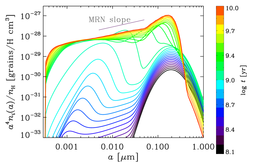
Figure 1: Evolution of grain size distribution. We present the case for silicate, but a similar evolutionary sequence is also obtained for carbonaceous dust. The grain size distribution is multiplied by $a^{4}$ and divided by $n_{\mathrm{H}}$ so that the resulting quantity is proportional to the dust mass in logarithmic bins per gas mass. The colour indicates the age as shown in the colour bar. The slope of the MRN grain size distribution is shown by the thin solid line for reference.

The effects of $\eta_{\mathrm{dense}}$ and $\tau_{\mathrm{SF}}$ are also shown and discussed in HM20. They are summarized as follows. If $\eta_{\mathrm{dense}}$ is smaller, coagulation becomes less efficient so that small grains less efficiently stick to form large grains. As a consequence, the grain size distributions at later times ($t\sim 3$–10 Gyr) are more dominated by small grains for smaller $\eta_{\mathrm{dense}}$. The opposite trend is observed for larger $\eta_{\mathrm{dense}}$; that is, the grain size distribution extends to larger grain radii. If we adopt $\eta_{\mathrm{dense}}=0.1$ (0.9), the upper cut-off of grain radius is located at $a\sim 0.08$ (0.8) $\micron$ for silicate; 0.04 (0.8) $\micron$ for carbonaceous dust. The other parameter, $\tau_{\mathrm{SF}}$, effectively regulates the speed of metal enrichment by stars. Faster enrichment overall leads to quicker dust evolution; however, since the time-scale of interstellar processing of dust does not scale with $\tau_{\mathrm{SF}}$ under a given metallicity, quicker metal enrichment means that the rate of interstellar processing catches up with that of metal enrichment at higher metallicity. This is most clearly seen in the evolution of dust-to-gas ratio as we will present in Section 3.3. As mentioned in HM20 (see also Asano et al. 2013a), a similar functional shape of grain size distribution is realized at the same value of $t/\tau_{\mathrm{SF}}^{1/2}$: this means that, since $Z\propto t/\tau_{\mathrm{SF}}$ approximately holds, a similar grain size distribution is realized at the same value of $Z\tau_{\mathrm{SF}}^{1/2}$, confirming the above statement that the modification of grain size distribution by interstellar processing occurs at higher metallicity for shorter $\tau_{\mathrm{SF}}$.

3.2 Dependence on $\eta_{\mathrm{dense}}$

We investigate the evolution of H₂ and CO abundances under various values of $\eta_{\mathrm{dense}}$, which regulates the grain size distribution. We adopt the fiducial values for the parameters of the cloud properties ($N_{\mathrm{H}}=10^{22}$ cm^-3, $\chi=1.7$, $n_{\mathrm{H,cl}}=10^{3}$ cm^-2, $T_{\mathrm{cl}}=10$ K, and $\Delta v=3$ km s^-1). In Fig. 2, we show the metallicity dependence of the molecular abundances and the CO-to-H₂ conversion factor. $X_{\mathrm{CO}}$ is only shown where $f_{\mathrm{CO}}>10^{-10}$, since it is not meaningful to show $X_{\mathrm{CO}}$ below such a low undetectable CO abundance. These quantities are shown as a function of metallicity, which is used as an indicator of galaxy evolution.

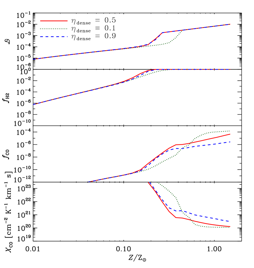
Figure 2: Panels from upper to lower show the dust-to-gas ratio ($\mathcal{D}$), H₂ fraction ($f_{\mathrm{H_{2}}}$), CO fraction ($f_{\mathrm{CO}}$) and CO-to-H₂ conversion factor ($X_{\mathrm{CO}}$) as functions of metallicity ($Z$). The solid, dotted, and dashed lines show the results for $\eta_{\mathrm{dense}}=0.5$ (fiducial), 0.1, and 0.9, respectively. $X_{\mathrm{CO}}$ is presented only when $f_{\mathrm{CO}}>10^{-10}$. For parameters other than $\eta_{\mathrm{dense}}$, we adopt the fiducial values.

The evolution of $\mathcal{D}$ is affected by $\eta_{\mathrm{dense}}$ (the first panel in Fig. 2). In particular, the metallicity at which $\mathcal{D}$ steeply increases depends on $\eta_{\mathrm{dense}}$: $Z\sim 0.2$–0.3 Z_☉ for $\eta_{\mathrm{dense}}=0.5$ and 0.9, and $Z\sim 0.3$–0.4 Z_☉ for $\eta_{\mathrm{dense}}=0.1$. This steep increase of $\mathcal{D}$ is due to dust growth by accretion. Below this metallicity, the dust is predominantly supplied by stars. If $\eta_{\mathrm{dense}}$ is as small as 0.1, the fraction of the dense ISM, which hosts accretion, is small. This leads to a low efficiency of accretion, delaying the increase of $\mathcal{D}$. In this context, the case with $\eta_{\mathrm{dense}}=0.9$ should show the most efficient dust growth; however, the accretion of gas-phase metals most efficiently occurs for small grains, whose production by shattering is the most inefficient in the case of the largest $\eta_{\mathrm{dense}}$ (because of the lowest fraction of the diffuse ISM hosting shattering). Because of these two counteracting effects, the metallicity at which $\mathcal{D}$ rapidly increases is not different between the cases with $\eta_{\mathrm{dense}}=0.9$ and 0.5. At low and high $Z$, $\mathcal{D}$ does not depend on $\eta_{\mathrm{dense}}$ because at low $Z$, the stellar dust production, which is independent of $\eta_{\mathrm{dense}}$, dominates the dust mass increase and at high $Z$, the dust-to-metal ratio is saturated to the maximum value $\mathrm{(D/Z)_{max}}$.

The H₂ fraction ($f_{\mathrm{H_{2}}}$) in the typical dense cloud also increases with metallicity (the second panel in Fig. 2). In the fiducial case ($\eta_{\mathrm{dense}}=0.5$), the increase of $f_{\mathrm{H_{2}}}$ is accelerated at $Z\gtrsim 0.1$ Z_☉ and $f_{\mathrm{H_{2}}}$ approaches 1 at $Z\sim 0.2$ Z_☉. At $Z\sim 0.1$ Z_☉ ($t\sim 0.7$ Gyr), the abundance of small grains starts to increase significantly by shattering and accretion (Fig. 1). This accelerates the increase in the surface area, raising the H₂ formation rate. Self-shielding of H₂ further increases the H₂ abundance by suppressing the H₂ dissociation. Although dust shielding also increases in this phase, it does not play a significant role in increasing the H₂ abundance. Indeed, we confirm (not shown in the figure) that there is little difference in $f_{\mathrm{H_{2}}}$ between the cases with and without dust shielding (i.e. applying $\tau_{\mathrm{LW},i}=0$ for the latter). The importance of self-shielding is also addressed by a hydrodynamic simulation which included the evolution of both grain size distribution and H₂ formation (Romano et al., 2022b). The H₂ fraction also depends on $\eta_{\mathrm{dense}}$: for $\eta_{\mathrm{dense}}=0.1$, the increase of small grains by accretion is delayed, so that the increase of $f_{\mathrm{H_{2}}}$ also occurs at a later stage. Since shattering is slower for $\eta_{\mathrm{dense}}=0.9$ than for $\eta_{\mathrm{dense}}=0.5$, the increase of $f_{\mathrm{H_{2}}}$ is slightly delayed for the larger value of $\eta_{\mathrm{dense}}$.

The CO fraction ($f_{\mathrm{CO}}$) in the typical dense cloud increases with metallicity (the third panel in Fig. 2). The metallicity at which $f_{\mathrm{CO}}$ steeply increases corresponds to the phase in which dust growth by accretion starts to play a significant role in increasing the dust abundance ($Z\sim 0.2$ Z_☉ in the fiducial case). Thus, dust shielding is important for the increase of $f_{\mathrm{CO}}$. In Appendix A, we examine the effect of each shielding source. The results are shown in Fig. 7. If we calculate $f_{\mathrm{CO}}$ without dust extinction ($A_{V,\mathrm{eff}}=0$), the CO abundance is significantly underpredicted. H₂ shielding plays a minor but appreciable role after the cloud becomes fully molecular, while CO self-shielding becomes as effective as H₂ shielding only after the increase of $f_{\mathrm{CO}}$ at $Z\sim 0.3$ Z_☉ (Fig. 7).

As we observe in Fig. 2, the $f_{\mathrm{CO}}$–$Z$ relation varies with $\eta_{\mathrm{dense}}$. In the case of $\eta_{\mathrm{dense}}=0.1$, the increase of $f_{\mathrm{CO}}$ occurs at a later stage because the increase of dust abundance occurs later. At high metallicity, $f_{\mathrm{CO}}$ eventually reaches a higher value for $\eta_{\mathrm{dense}}=0.1$ than for higher $\eta_{\mathrm{dense}}$. This is because the dust extinction is enhanced if the grain size distribution is biased towards smaller sizes. The grain size effect is more effectively seen if we compare the results for $\eta_{\mathrm{dense}}=0.5$ and 0.9. Although the evolution of dust-to-gas ratio is similar between these two cases, the resulting $f_{\mathrm{CO}}$ is differentiated because of the difference in the grain size distribution. The grain size distribution is more biased to larger grains for $\eta_{\mathrm{dense}}=0.9$ than for $\eta_{\mathrm{dense}}=0.5$, leading to less efficient shielding of dissociating radiation. Therefore, the evolution of grain size distribution and dust abundance has a large impact in the metallicity dependence of $f_{\mathrm{CO}}$.

As expected from the sensitive hevaviour of $f_{\mathrm{CO}}$ to the grain evolution, the CO-to-H₂ conversion factor, $X_{\mathrm{CO}}$, is greatly affected by $\eta_{\mathrm{dense}}$ (the bottom panel in Fig. 2). First of all, $X_{\mathrm{CO}}$ is sensitive to metallicity as already shown by other studies (see the Introduction). The change of $X_{\mathrm{CO}}$ particularly occurs in the metallicity range where the cloud is rich in H₂ but is not rich in CO. $X_{\mathrm{CO}}$ approaches the Milky Way value ($\sim 2\times 10^{20}$ cm^-2 K^-1 km^-1 s; Bolatto et al. 2013) at nearly solar metallicity. The decrease of $X_{\mathrm{CO}}$ towards high metallicity roughly traces the increasing trend of $f_{\mathrm{CO}}$. The different tracks for the different values of $\eta_{\mathrm{dense}}$ also follows the trends in $f_{\mathrm{CO}}^{-1}$. The conversion factor stays relatively high for $\eta_{\mathrm{dense}}=0.9$, while it drops down to $\sim 10^{20}$ cm^-2 K^-1 km^-1 s for the other cases.

3.3 Dependence on $\tau_{\mathrm{SF}}$

We examine the dependence on the star formation time-scale $\tau_{\mathrm{SF}}$, which regulates the speed of metal enrichment. We show the resulting metallicity dependences of $\mathcal{D}$, $f_{\mathrm{H_{2}}}$, $f_{\mathrm{CO}}$ and $X_{\mathrm{CO}}$ in Fig. 3.

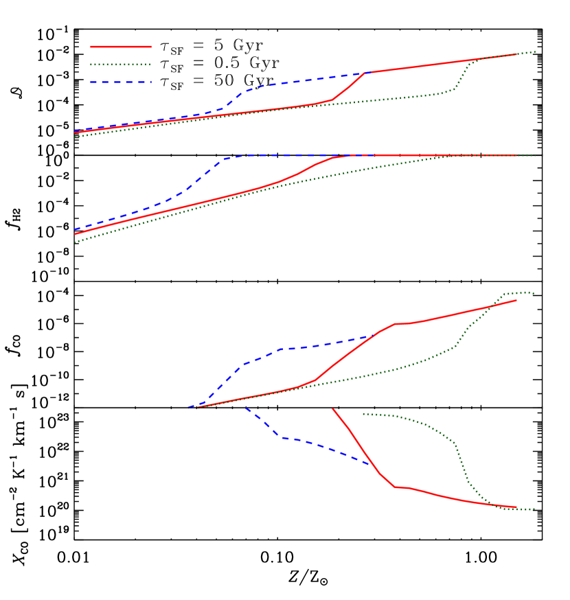
Figure 3: Same as Fig. 2 but for the dependence on $\tau_{\mathrm{SF}}$. We adopt the fiducial values for other parameters. The solid dotted, and dashed lines show the results for $\tau_{\mathrm{SF}}=5$ (fiducial), 0.5, and 50 Gyr, respectively.

Overall, the effect of $\tau_{\mathrm{SF}}$ is to determine the metallicity level at which steep increases of $\mathcal{D}$, $f_{\mathrm{H_{2}}}$, and $f_{\mathrm{CO}}$ occur. This is because, as mentioned in Section 3.1, a similar grain size distribution is approximately achieved at the same value of $Z\tau_{\mathrm{SF}}^{1/2}$ (Section 3.1). Thus, the evolution of each quantity is ‘shifted’ towards high metallicity as $\tau_{\mathrm{SF}}$ becomes shorter.

Since the drop of $X_{\mathrm{CO}}$ coincides with the rise of $f_{\mathrm{CO}}$, the metallicity level at which $X_{\mathrm{CO}}$ drops is strongly affected by $\tau_{\mathrm{SF}}$. In particular, if $\tau_{\mathrm{SF}}$ is as short as 0.5 Gyr, $X_{\mathrm{CO}}$ changes sharply from a large value to the MW-like one at solar metallicity. This means that it is difficult to detect CO from rapidly ($\tau_{\mathrm{SF}}\lesssim 0.5$ Gyr) star-forming galaxies if the metallicity is lower than solar. In nearby starbursts, CO is usually detected probably because they are already sufficiently metal/dust enriched in the current or previous star formation episodes.

Here we note that treating $\tau_{\mathrm{SF}}$ as a completely free parameter could enhance the effect of $\tau_{\mathrm{SF}}$ on the $\mathcal{D}$–$Z$ relation. HH17 did not treat $\tau_{\mathrm{SF}}$ as a completely independent parameter but linked it to the accretion time-scale. This is because both accretion (dust growth) and star formation occur in the dense ISM. In contrast, our present model gives the dense gas fraction $\eta_{\mathrm{dense}}$ (note that accretion efficiency is weighted with $\eta_{\mathrm{dense}}$ in our approach; Section 2.1) as a free parameter, and does not relate it to $\tau_{\mathrm{SF}}$. These different approaches produce different results in the following point: in HH17’s treatment, the evolution of $\mathcal{D}$ is hardly affected by $\tau_{\mathrm{SF}}$ because of the proportionality between the time-scales of star formation and accretion. In our model, in contrast, the $\mathcal{D}$–$Z$ relation is strongly affected by $\tau_{\mathrm{SF}}$. However, we should also note that HH17’s treatment needs to introduce another free parameter: star formation efficiency. Probably, the realistic situation lies between these two treatments, and can only be treated in a more ‘realistic’ model such as hydrodynamic simulations that could predict the formation of dense clouds and star formation consistently.

3.4 Comparison with observations

We compare the above calculation results with observations. In particular, data for the dust-to-gas ratio and the CO-to-H₂ conversion factor are available for nearby galaxies with different metallicities. We basically use the same observational data as adopted by HH17, who took the data sets compiled in Bolatto et al. (2013) and supplemented by Cormier et al. (2014) for low-metallicity galaxies. In addition to the $X_{\mathrm{CO}}$–$Z$ relation, we also show the $\mathcal{D}$–$Z$ relations, where the data are taken from Rémy-Ruyer et al. (2014). We adopt the dust-to-gas ratio estimated with a metallicity-dependent CO-to-H₂ conversion factor, which only has a minor influence on the resulting $\mathcal{D}$–$Z$ relation. Recent more elaborate analysis (e.g. Aniano et al., 2020; De Vis et al., 2021; Galliano et al., 2021) shows similar $\mathcal{D}$–$Z$ relations for nearby galaxies. To further supplement the data for $X_{\mathrm{CO}}$ at low metallicity, we also include the data from Shi et al. (2016), but do not show a galaxy (DDO70-A) with $Z<0.1$ Z_☉, where the gas mass estimate depends strongly on the assumption on the relation between dust-to-gas ratio and metallicity. By excluding this galaxy, we concentrate on the comparison at $Z>0.1$ Z_☉ as mentioned in Section 2.2.

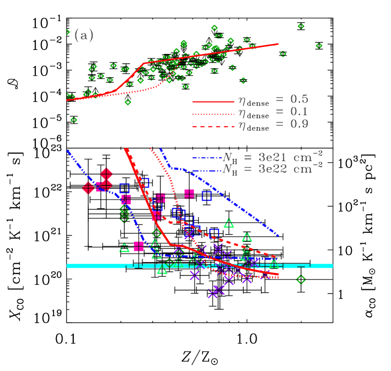
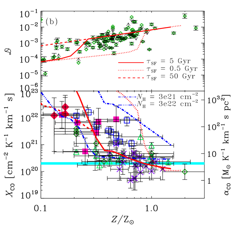
Figure 4: Relations between dust-to-gas ratio and metallicity (upper window in each panel) and between CO-to-H₂ conversion factor and metallicity (lower window). Panels (a) and (b) show the dependence on $\eta_{\mathrm{dense}}$ and $\tau_{\mathrm{SF}}$, whose values are the same as shown in Figs. 2 and 3, respectively (also shown in the legends). For $X_{\mathrm{CO}}$, we also plot the cases with lower and higher hydrogen column densities, $N_{\mathrm{H}}=3\times 10^{21}$ and $3\times 10^{22}$ cm^-2 by the dot–dashed and triple-dot–dashed lines, respectively, with $\eta_{\mathrm{dense}}=0.5$ and $\tau_{\mathrm{SF}}=5$ Gyr. The conversion factor is expressed in two units as shown on the left and right vertical axes. The points with error bars are the observation data in the literature: Rémy-Ruyer et al. (2014) in the upper window, and Leroy et al. (2011, open diamonds), Bolatto et al. (2008, triangles), Israel (1997, open squares), Sandstrom et al. (2013, crosses), Cormier et al. (2014, filled squares), and Shi et al. (2016, filled diamonds) in the lower window, where we also show the MW value of $X_{\mathrm{CO}}$ by the horizontal thick line as a reference.

In Fig. 4, we compare our results with the observational data for the $\mathcal{D}$–$Z$ and $X_{\mathrm{CO}}$–$Z$ relations. We observe that overall, the models nicely reproduce the increasing and decreasing trends in $\mathcal{D}$ and $X_{\mathrm{CO}}$, respectively. For the $\mathcal{D}$–$Z$ relation, the nonlinear trend (or the steep increase of $\mathcal{D}$ at subsolar metallicity) is caused by accretion, which is consistent with the observed trend of dust-to-metal ratio (Rémy-Ruyer et al., 2014). The observed $X_{\mathrm{CO}}$–$Z$ relation is also explained by the same models; in particular, the fiducial case is located in the middle of the observational data. The variation among the cases with $\eta_{\mathrm{dense}}=0.1$–0.9 also explains the scatter in the observed $\mathcal{D}$–$Z$ and $X_{\mathrm{CO}}$–$Z$ relations. As mentioned in Section 3.2, in spite of the almost same evolutionary track in the $\mathcal{D}$–$Z$ relations between $\eta_{\mathrm{dense}}=0.5$ and 0.9, these two cases have significantly different values of $X_{\mathrm{CO}}$ (originating from different $f_{\mathrm{CO}}$) at high metallicity because of different grain size distributions. Therefore, even if the dust-to-gas ratio is similar, the CO-to-H₂ conversion factor can be very different because of different grain size distributions. The high and low values of $\tau_{\mathrm{SF}}$ explain the variations at high and low metallicities, respectively. This is because the metallicity at which the prominent increase of $\mathcal{D}$ occurs is shifted towards high and low metallicities for short and long $\tau_{\mathrm{SF}}$, respectively.

As shown in HH17, the hydrogen column density $N_{\mathrm{H}}$ of the cloud can also produce a large variation in the $X_{\mathrm{CO}}$–$Z$ relation. Thus, in Fig. 4, we consider an order of magnitude variation centred at the fiducial value; that is, we examine $N_{\mathrm{H}}=3\times 10^{21}$ and $3\times 10^{22}$ cm^-2 in addition to the fiducial case. Note that $N_{\mathrm{H}}$ does not affect the $\mathcal{D}$–$Z$ relation. We overall find that the above range of $N_{\mathrm{H}}$ is consistent with the range (or the scatter) of $X_{\mathrm{CO}}$ in the observational data. As expected, the larger and smaller values of $N_{\mathrm{H}}$ predict higher and lower values of $f_{\mathrm{CO}}$, leading to lower and higher values of $X_{\mathrm{CO}}$, respectively, except at high metallicity. At solar metallicity and above, $X_{\mathrm{CO}}$ is higher for $N_{\mathrm{H}}=3\times 10^{22}$ cm^-2 than for $N_{\mathrm{H}}=10^{22}$ cm^-2 because the saturation of the CO line intensity due to high optical depth is more prominent at higher $N_{\mathrm{H}}$. This means that, at high metallicity, $N_{\mathrm{H}}\sim 10^{22}$ cm^-2 is the optimum column density for the CO $J=1\to 0$ emission intensity per hydrogen, and the higher and lower column densities both lead to less efficient emission.

In Fig. 4, we also show the MW value of $X_{\mathrm{CO}}$ as a reference. We observe that the fiducial model ($\eta_{\mathrm{dense}}=0.5$ and $\tau_{\mathrm{SF}}=5$ Gyr) reaches the MW value at solar metallicity, which is appropriate for the metallicity of the MW. This confirms that our grain evolution model predicts a conversion factor consistent with the observed one at solar metallicity if we choose standard values for relevant parameters. We should still be aware of possible systematic errors that could cause offsets for the observationally obtained $X_{\mathrm{CO}}$. At the same time, our model also contains adjustable parameters such as $T_{\mathrm{cl}}$ and $\Delta v$. In spite of these systematic errors and adjustments, we still firmly conclude that our model is capable of reproducing the trend in the $X_{\mathrm{CO}}$–$Z$ relation well.

As expected from the above results, a large fraction of carbon atoms in dense gas are traced by emission not from CO but from other forms of carbon such as C ii and C i at low metallicity (e.g. Madden et al., 1997; Cormier et al., 2014; Glover & Clark, 2016; Hu et al., 2021). The transition of C ii/C i-dominated to CO-dominated carbon content occurs at $Z\sim 0.2$–0.3 Z_☉ in our fiducial model. This corresponds to the metallicity at which dust growth by accretion causes a rapid increase of the dust abundance. We note that dust shielding, which helps CO formation, is further enhanced by efficient small-grain production around this metallicity.

4 Discussion

4.1 Dust-based conversion factor formulae

The above results indicate that the dust abundance and the grain size distribution have large impact on the CO-to-H₂ conversion factor. This motivates us to further analyze the relation between $X_{\mathrm{CO}}$ and dust-related quantities. Here we reanalyze our results in terms of the dust-to-gas ratio $\mathcal{D}$ and the grain size distribution.

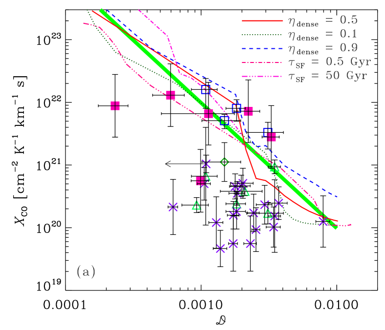
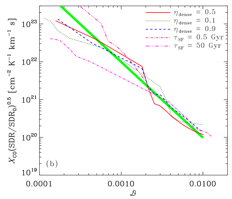
Figure 5: (a) CO-to-H₂ conversion factor as a function of dust-to-gas ratio. The (thin) solid, dotted, and dashed curves present the cases with $\eta_{\mathrm{dense}}=0.5$ (fiducial), 0.1, and 0.9, respectively, while the dot–dashed, and triple-dot–dashed lines show the results with $\tau_{\mathrm{SF}}=0.5$ and 5 Gyr, respectively. The parameters other than the varied one are fixed to the fiducial values. The thick light green line is the proposed power-law formula in equation (16). (b) The relations shown is Panel (a) is corrected for the $(\mathrm{SDR}/\mathrm{SDR}_{0})^{0.5}$ factor, which includes the information on the grain size distribution, to minimize the variety at high metallicity. The models are the same as in Panel (a), and the thick green line shows the proposed power-law formula in equation (18) with $\mathrm{SDR}=\mathrm{SDR}_{0}$.

First we examine how $X_{\mathrm{CO}}$ is related to the dust abundance represented by the dust-to-gas ratio $\mathcal{D}$. In Fig. 5a, we show $X_{\mathrm{CO}}$ as a function of dust-to-gas ratio $\mathcal{D}$. We present various models investigated above: the variation of $\eta_{\mathrm{dense}}$ and $\tau_{\mathrm{SF}}$. The parameters other than the varied one are fixed to the fiducial values. We observe in the figure that the conversion factor $X_{\mathrm{CO}}$ is better aligned in a single sequence if we plot it as a function of $\mathcal{D}$ instead of $Z$. Overall, $X_{\mathrm{CO}}$ can be approximated by a power-law function of $\mathcal{D}$ with a single slope, while it had a clear kink when it was plotted as a function of $Z$ (Figs. 2 and 3). We suggest the following formula roughly reproducing the trends in all the models shown:

$$X_{\mathrm{CO}}=2\times 10^{20}\left(\frac{\mathcal{D}}{7\times 10^{-3}}\right)^{-2}~{}\mathrm{cm^{-2}~{}\mathrm{K}^{-1}~{}km^{-1}~{}s},$$ (16)

which is obtained with a constraint that the MW dust-to-gas ratio $\mathcal{D}=7\times 10^{-3}$ (Weingartner & Draine, 2001; Hirashita, 2023) reproduces the MW value of $X_{\mathrm{CO}}$ as well as a requirement that the overall trend traces all the models shown. The conversion factors in all the models are broadly consistent with this suggested formula within a factor of 3.

We also show the observational data for comparison in Fig. 5a. We adopt the same sample as in Fig. 4 but only plot galaxies whose dust-to-gas ratio is available from Rémy-Ruyer et al. (2014); i.e. we use the consistent values of dust-to-gas ratio with the upper windows of Fig. 4. We note that the comparison is not fully consistent because most observational data are analyzed with different assumptions on the dust-to-metal (or dust-to-gas) ratio in evaluating $X_{\mathrm{CO}}$ or on the CO-to-H₂ conversion factor in estimating $\mathcal{D}$. For uniformity of the data, the estimated values of $\mathcal{D}$ are taken from a single paper. We observe that the data from Sandstrom et al. (2013), which are shown by crosses, are systematically located at lower $X_{\mathrm{CO}}$ compared with the points from Israel (1997) and Cormier et al. (2014). Note that the latter two papers assumed relations between dust and gas masses (or emissions). Sandstrom et al. (2013) did not assume any relation between gas and dust masses, and find self-consistent values of $X_{\mathrm{CO}}$ and $\mathcal{D}$ in their spatially resolved galaxy maps under an assumption that the correct solution should minimize the dispersion of $\mathcal{D}$ within a kpc-scale region. Although this assumption is plausible, a further study is necessary to understand possible bias by cross-checking various methods.

We showed above that the grain size distribution plays an important role in the CO abundance. To obtain a simple quantity that characterizes the grain size distribution, we first define the following weighted integral of a function $f(a)$ for the grain size distribution:

$$I(f)\equiv\sum_{i}\int_{0}^{\infty}f_{i}(a)n_{i}(a)\,\mathrm{d}a,$$ (17)

where the index $i$ specifies the grain species. A simple example is a series of moments: $f(a)=a^{\ell}$ ($\ell=0$, 1, 2, $\cdots$) as used by Mattsson (2016). Although the full moment treatment is out of the scope of this paper, a simple physical intuition may lead to the importance of the second and third moments ($\ell=2$ and 3), which are indicators of the grain surface area and volume, respectively. For the purpose of this paper, we take $S_{\mathrm{d}}(a)=\pi a^{2}$ and $m_{\mathrm{d}}(a)=4\pi a^{3}s/3$ for the function $f(a)$ above. The dust-to-gas ratio is expressed as $\mathcal{D}=I(m_{\mathrm{d}})/(1.4m_{\mathrm{H}}n_{\mathrm{H}})$ and the grain surface area per gas mass, denoted as $\mathcal{S}$, is calculated by $\mathcal{S}=I(S_{\mathrm{d}})/(1.4m_{\mathrm{H}}n_{\mathrm{H}})$, where the factor 1.4 indicates the correction for helium. Using these two quantities, the surface-to-mass ratio of the dust is obtained as $\mathcal{S}/\mathcal{D}$. Because the grain surface area can be used as an indicator of the opacity for dissociating radiation (although the relation is not completely proportional), we try to use the ‘SD ratio’ defined as $\mathrm{SDR}\equiv\mathcal{S}/\mathcal{D}$ as a quantity that reflects the main effect of the grain size distribution.

Since $X_{\mathrm{CO}}$ is affected by the grain size distribution in addition to the dust abundance, we propose that $X_{\mathrm{CO}}\propto(\mathrm{SDR})^{\gamma}F(\mathcal{D})$, where $F(\mathcal{D})$ is a function of $\mathcal{D}$. In other words, the explicit dependence on the grain size distribution is assumed to be expressed by a power-law function of SDR for simplicity. With this assumption, $X_{\mathrm{CO}}(\mathrm{SDR})^{-\gamma}$ is a function of $\mathcal{D}$ not explicitly dependent on the shape of grain size distribution. After some tests, $\gamma\sim-0.5$ minimizes the dispersion among the models at high metallicity (where the CO detection is actually expected). In our fiducial model, $\mathrm{SDR}=2.9\times 10^{5}$ cm² g^-1 at the MW dust-to-gas ratio ($\mathcal{D}=7\times 10^{-3}$).

In Fig. 5, we show $X_{\mathrm{CO}}(\mathrm{SDR}/\mathrm{SDR}_{0})^{0.5}$, where $\mathrm{SDR}_{0}=2.9\times 10^{5}$ cm² g^-1 is used for normalization based on our fiducial model, as a function of $\mathcal{D}$. We confirm that the dispersion among the models at high metallicity becomes significantly smaller if we present $X_{\mathrm{CO}}(\mathrm{SDR}/\mathrm{SDR}_{0})^{0.5}$ instead of $X_{\mathrm{CO}}$. In the figure, we also show the corrected version of equation (16):

$$X_{\mathrm{CO}}=2\times 10^{20}\left(\frac{\mathcal{D}}{7\times 10^{-3}}\right)^{-2}~{}\left(\frac{\mathrm{SDR}}{\mathrm{SDR}_{0}}\right)^{-0.5}\mathrm{cm^{-2}~{}\mathrm{K}^{-1}~{}km^{-1}~{}s}.$$ (18)

This formula is useful if both dust-to-gas ratio and SDR are available or can be reasonably assumed. It is, however, usually difficult to obtain the information on the dust surface area; in this case, we could fix SDR to our fiducial value ($\mathrm{SDR}_{0}$), and the relation is reduced to equation (16).

Since dust plays a more prominent role in regulating the CO abundance than metals, it may be more robust to use the dust-based formulae proposed in equation (16) or (18). However, the usefulness of these formulae is not obvious in the following two points: (i) For the gas mass estimate necessary to obtain the dust-to-gas ratio, we need $X_{\mathrm{CO}}$; thus, the process of estimating dust-to-gas ratio with an undetermined value of $X_{\mathrm{CO}}$ is iterative. (ii) The relation is not yet observationally supported in a robust way. Seeing Fig. 5a, there are a significant number of data points deviating from the proposed relation. However, the observational estimate of $X_{\mathrm{CO}}$ also needs some assumptions. Thus, further cross-checks among the observational methods of deriving $X_{\mathrm{CO}}$ are necessary to understand possible systematic errors in each data set.

4.2 Possible dependence on other parameters

As mentioned in Section 2.5, some of the physical parameters for the typical cloud may affect the results. In particular, the gas temperature and the ISRF are expected to have a large variety depending on the star formation activity and the detailed spatial distributions of stars and clouds in the galaxy. Thus, we examine the variation of cloud parameters. Since we already investigated the effect of $N_{\mathrm{H}}$ in Section 3.4, we fix it to the fiducial value ($N_{\mathrm{H}}=10^{22}$ cm^-2).

Starburst galaxies have SFR surface densities up to $\sim 10^{4}$ times higher than normal spiral galaxies (Kennicutt, 1998). Assuming that the ISRF intensity is proportional to the SFR surface density, we examine $\chi$ up to $1.7\times 10^{4}$. In Fig. 6, we show the results for $\chi=1.7$, $1.7\times 10^{2}$ and $1.7\times 10^{4}$ with other parameters fixed to the fiducial values. Note that the evolution of $\mathcal{D}$ is not affected by $\chi$. We observe in the figure that the H₂ and CO abundances are suppressed in high radiation fields at low metallicity. The cloud, however, achieves $f_{\mathrm{H_{2}}}\sim 1$ at $Z\gtrsim 0.3$ Z_☉, and this metallicity is not sensitive to $\chi$. The ISRF intensity also affects $f_{\mathrm{CO}}$ at low metallicity, but its effect is less at high metallicity because a large fraction of the ISRF is shielded by dust. Accordingly, the CO-to-H₂ conversion factor has a large variety at low metallicity, while the difference becomes moderate at high metallicity. Indeed, $X_{\mathrm{CO}}$ varies only by a factor of $\sim$3 at solar metallicity although $\chi$ differs by four orders of magnitude.

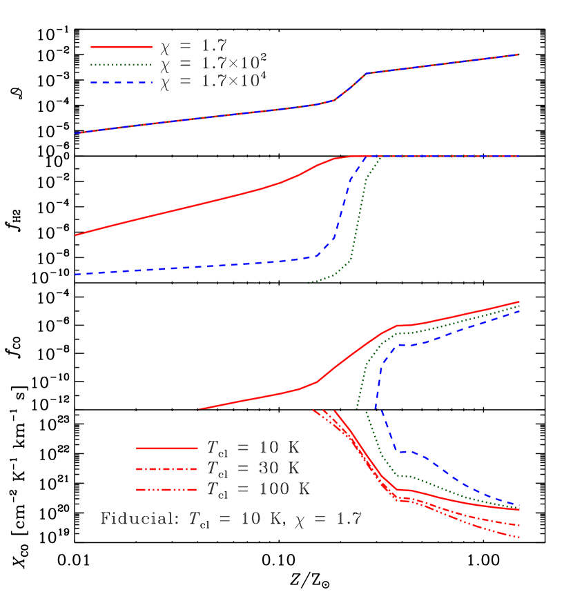
Figure 6: Same as Fig. 2 but for different values of for $\chi$ (1.7, $1.7\times 10^{2}$ and $1.7\times 10^{4}$; solid, dotted and dashed lines, respectively) with $T_{\mathrm{cl}}=10$ K. We also show $X_{\mathrm{CO}}$ for $T_{\mathrm{cl}}=30$ and 100 K with $\chi=1.7$ (dot–dashed and triple-dot–dashed lines, respectively). Note that $T_{\mathrm{cl}}$ prominently affects $X_{\mathrm{CO}}$, so that the $T_{\mathrm{cl}}$ dependence is only shown in the bottom panel. Neither $\chi$ nor $T_{\mathrm{cl}}$ influences the evolution of $\mathcal{D}$. For the parameters other than the varied one, we adopt the fiducial values.

In Fig. 6, we also show the dependence on $T_{\mathrm{cl}}$. Note that the prominent effect of $T_{\mathrm{cl}}$ is only seen for the CO-to-H₂ conversion factor in our model, so that the $T_{\mathrm{cl}}$-dependence is only shown for $X_{\mathrm{CO}}$. We observe that $T_{\mathrm{cl}}$ little affects $X_{\mathrm{CO}}$ at low metallicity because $W_{\mathrm{CO}}$ is insensitive to $T_{\mathrm{cl}}$ (Section 2.5). At high metallicity, the line emission becomes optically thick, which leads to the CO line intensity almost proportional to $T_{\mathrm{cl}}$. Thus, $X_{\mathrm{CO}}$ is lower for higher $T_{\mathrm{cl}}$ at high metallicity. Variation of $\Delta v$ (not shown in the figure) also has a similar effect to that of $T_{\mathrm{cl}}$.

Starburst galaxies such as (ultra)luminous infrared galaxies have lower $X_{\mathrm{CO}}\sim 0.2$–$1\times 10^{20}$ cm^-2 K^-1 km^-1 s, than that in the MW (see section 7 of Bolatto et al., 2013, for a review). As supported by the above results, the low conversion factors in starburst galaxies could be explained by high gas temperatures (Wild et al., 1992) or high velocity dispersions (Zhu et al., 2003; Papadopoulos et al., 2012) or both (Narayanan et al., 2011). The high radiation field may have a less significant influence on $X_{\mathrm{CO}}$ if these galaxies have nearly solar metallicity.

Although our model has been compared with nearby galaxies, it is also applicable to high-redshift galaxies. Tacconi et al. (2008) observed CO lines from submillimetre galaxies (SMGs) and UV/optically selected galaxies at $z\sim 2$. Their most favoured solution indicates that the CO-to-H₂ conversion factors of the SMGs are similar to nearby ULIRGs while those of the UV/optically selected galaxies are near to the MW value. Daddi et al. (2010) also showed that the CO-to-H₂ conversion factors of the main-sequence galaxies at $z\sim 1.5$ are near the MW value. Magdis et al. (2011) also found a difference in the conversion factor between a SMG and a main-sequence galaxy. Magnelli et al. (2012) showed a negative correlation between CO-to-H₂ conversion factor and dust temperature for galaxies at $z\sim 1$. The dust temperature is expected to be positively correlated with $\chi$; however, higher $\chi$ predicts larger $X_{\mathrm{CO}}$ in our model (Fig. 6), which is opposite to the observed trend. Since their sample has solar metallicity, the difference in $X_{\mathrm{CO}}$ could be more prominently caused by the variation in gas temperature or velocity dispersion as discussed above (see also Maloney & Black, 1988).

Our results also imply difficulty in detecting CO at $z\gtrsim 5$ when the cosmic age is $\lesssim 1$ Gyr. We expect that many of the galaxies at $z\gtrsim 5$ are metal-poor, which indicates that CO is difficult to detect because $X_{\mathrm{CO}}$ is large. Our result in Section 3.3 further indicates that galaxies with short $\tau_{\mathrm{SF}}$ have a sharp transition from large to small $X_{\mathrm{CO}}$ at solar metallicity. Thus, even if a galaxy at $z\gtrsim 5$ experiences a quick metal enrichment (i.e. has a short $\tau_{\mathrm{SF}}$), it is not necessarily CO-rich. The transition from a CO-poor to CO-rich galaxy occurs in a narrow range of metallicity. This may predict that high-redshift galaxies are ‘bimodal’ in the CO-rich and CO-poor phases. Since this transition is related to the dust growth by accretion, we also predict that this CO-rich/poor bimodality is associated with the dust-rich/poor distinction. If the fraction of galaxies with short $\tau_{\mathrm{SF}}$ is large at high redshift, it is important to use [C ii] and/or [C i] emission to trace star-forming gas in galaxies.

4.3 Conversion factor prescriptions

Most of the prescriptions for the conversion factor include the metallicity dependence. Many of them adopted a power-law metallicity dependence of $X_{\mathrm{CO}}$ (e.g. Israel, 1997; Schruba et al., 2012; Hunt et al., 2015; Accurso et al., 2017). These power-law dependences are broadly consistent with the observational data shown in Fig. 4. From a physical insight from the fraction of CO-dark molecular gas, exponential dependence may be expected (Wolfire et al., 2010; Bolatto et al., 2013). Because of the large scatter in the observational data, we are not able to judge which functional form of $X_{\mathrm{CO}}$ describes the observations better.

Our results show that the $X_{\mathrm{CO}}$–$Z$ relation is also affected by the dust evolution. If we focus on $Z\gtrsim 0.3$ Z_☉, $X_{\mathrm{CO}}$ could be approximated by a power law, while the sharp rise towards lower metallicity may be better described by a steeper function. The sharp decrease of $X_{\mathrm{CO}}$ is associated with the change of the major dust sources from stellar dust production to dust growth by accretion. Thus, to describe the $X_{\mathrm{CO}}$–$Z$ relation in a wide metallicity range, it is crucial to understand or model the dust evolution.

Note again that $X_{\mathrm{CO}}$ also depends on quantities other than the metallicity and the grain size distribution. Bolatto et al. (2013) suggested that $X_{\mathrm{CO}}$ depends on the surface density of total baryons ($\Sigma_{\mathrm{tot}}$) as $X_{\mathrm{CO}}\propto\Sigma_{\mathrm{tot}}^{-0.5}$ at high $\Sigma_{\mathrm{tot}}(>100~{}\mathrm{M}_{\sun}~{}\mathrm{pc}^{-2})$ such as realized in galaxy centres. Chiang et al. (2021) showed that the $\Sigma_{\mathrm{tot}}$-dependent $X_{\mathrm{CO}}$ is preferred to obtain reasonable radial profiles of dust-to-metal ratio for a sample of nearby galaxies. The $\Sigma_{\mathrm{tot}}$ dependence is probably due to the difference in the physical conditions regulated by the gravity. In particular, as shown above, the temperature and the velocity dispersion of the cloud affect $X_{\mathrm{CO}}$ if CO is optically thick (Section 4.2). It is natural to consider that $\Delta v^{2}$ and $T_{\mathrm{cl}}$ reflect the depth of the gravitational potential, which is proportional to $\Sigma_{\mathrm{tot}}$. Thus, we hypothesize that $\Delta v^{2}\propto\Sigma_{\mathrm{tot}}^{p}$ and $T_{\mathrm{cl}}\propto\Sigma_{\mathrm{tot}}^{q}$ with $p>0$ and $q>0$. We also assume that the molecular gas surface density, $\Sigma_{\mathrm{mol}}$ positively correlates with $\Sigma_{\mathrm{tot}}$: $\Sigma_{\mathrm{mol}}\propto\Sigma_{\mathrm{tot}}^{r}$ with $r>0$. With these assumptions, we obtain $X_{\mathrm{CO}}\propto\Sigma_{\mathrm{mol}}/(T_{\mathrm{cl}}\Delta v)\propto\Sigma_{\mathrm{tot}}^{(r-0.5p-q)}$ at high optical depth (at high metallicity). Thus, if $r-0.5p-q=-0.5$, the above surface density dependence can be explained. For example, if we assume simple proportionality for all the relations (i.e. $p=q=r=1$), the above relation is satisfied. Although further sophisticated dynamical modelling would be required to obtain more precise values of $p$, $q$ and $r$ (see also section 2 of Bolatto et al., 2013), the above simple argument implies that the dependence on the total surface density can be translated into that on the gas density and velocity dispersion investigated in Section 4.2.

Our one-zone approach is not capable of calculating the physical conditions of dense clouds in a consistent manner with the hydrodynamic evolution of the ISM. Hydrodynamic simulations provide a viable method for predicting physical quantities that govern the H₂ and CO abundances. Some hydrodynamic simulations of galaxies included the evolution of grain size distribution. In particular, Aoyama et al. (2020) showed that the grain size distributions are systematically different between the dense and diffuse ISM. Thus, our assumption of identical grain size distribution everywhere in the galaxy may need to be modified. However, Romano et al. (2022a), using the same simulation framework but including turbulent diffusion, showed that the grain size distribution can be homogenized between the dense and diffuse ISM. This means that a one-zone model could provide a reasonable description if the diffusion is strong. The simple one-zone study in this paper will give a basis on which we interpret spatially resolved evolution in future simulations.

Another feature that a one-zone treatment is not able to predict is the variation within a galaxy. Hou et al. (2017) showed that the small-to-large grain abundance ratio varies with galactocentric distance (see e.g. Romano et al., 2022a, for a recent simulation). This variation is mainly driven by different metal enrichment (or star formation) histories. However, the evolutionary sequence of grain size distribution is similar to that predicted from a one-zone model with a delay in regions with slower metal enrichment (usually in the outer galactic discs). The spatial variation of CO-to-H₂ conversion factor is also an important topic to clarify using a frameworks that combines our models developed in this paper and hydrodynamic simulations.

4.4 Possible impacts of inhomogeneity in the cloud

Our treatment of H₂ abundance is based on a uniform density and a homogeneous mixture between dust and gas. There are some effects that inhomogeneity could have on the H₂ abundance. Broadly, there are two types of effects: One is the effect of local density enhancement and the other is dust–gas decoupling.

In an inhomogeneous medium, the reaction rate is enhanced in regions where the density is higher than the average. The H₂ formation, which is proportional to the product of dust and gas densities, is enhanced by a factor of $\langle n_{\mathrm{H}}n_{\mathrm{d}}\rangle/\langle n_{\mathrm{d}}\rangle\langle n_{\mathrm{H}}\rangle$, where the bracket indicates the spatial average within the cloud, and $n_{\mathrm{H}}$ and $n_{\mathrm{d}}$ are the local number densities of hydrogen nuclei and dust grains, respectively. If dust and gas are tightly coupled (i.e. the dust-to-gas ratio is uniform), the above ratio is reduced to $\langle n_{\mathrm{H}}^{2}\rangle/\langle n_{\mathrm{H}}\rangle^{2}$. The density enhancement is related to the mean Mach number of the turbulence (e.g. Vazquez-Semadeni, 1994; Federrath et al., 2008); that is, the density enhancement is a dynamical phenomenon. Thus, we need to take into account the finite formation time of H₂, and evaluate the H₂ fraction in a manner consistent with the dynamical density evolution within the cloud. Although this dynamical treatment is not possible in our framework, our formulae for the H₂ formation rate including the effect of grain size distribution is generally applicable. Future development that combines the grain size distribution and the hydrodynamic evolution is necessary to address the local enhancement of H₂ formation rate in an inhomogeneous structure.

The assumption of homogeneous mixing between dust and gas also needs to be checked carefully. Hopkins & Lee (2016) showed that decoupling of dust grains from small-scale gas density structures could make significantly different spatial distributions between dust and gas. The resulting spatial distribution of dust is, however, affected by complex factors such as grain charging and magnetic field (Lee et al., 2017; Beitia-Antero et al., 2021; Moseley et al., 2023). Basically, the effect of decoupling would weaken the effect of local density enhancement: The enhancement factor for the H₂ formation rate is written as $\langle n_{\mathrm{H}}n_{\mathrm{d}}\rangle/\langle n_{\mathrm{d}}\rangle\langle n_{\mathrm{H}}\rangle$ as mentioned above, and is reduced to unity if dust and gas are independently distributed (i.e. $\langle n_{\mathrm{H}}n_{\mathrm{d}}\rangle=\langle n_{\mathrm{H}}\rangle\langle n_{\mathrm{d}}\rangle$). Thus, decoupling would tend to justify the usage of averaged quantities. However, detailed effects depend on the grain radius, so that it is interesting to further investigate the effect of decoupling on the H₂ formation by combining our grain size distribution model and dust–gas dynamic simulations in future work.

Compared with the formation rate, the dissociation rate of H₂ is less affected by inhomogeneity in density and dust-to-gas ratio for the following reasons. The optical depth for dissociating radiation reflects the mean density along the light path. although the precise shielding strength depends on the clumpiness and the optical depth of each clump (e.g. Városi & Dwek, 1999). The formation rate, in contrast, depends directly on the local density. Thus, we expect that density inhomogeneity affects the formation rate of H₂ much more than the destruction rate. Moreover, as mentioned in Section 3.2, self-shielding is the main shielding mechanism for H₂. Therefore, the detailed spatial distribution of dust is not important for shielding, which means that dust–gas decoupling has a minor influence on H₂ dissociation.

From the above discussions, it is possible that density inhomogeneity could enhance the H₂ abundance through the local enhancement of H₂ formation rate. Therefore, $f_{\mathrm{H_{2}}}$ could reach unity at lower metallicity than our results. This does not change our conclusion for $X_{\mathrm{CO}}$ since $f_{\mathrm{H_{2}}}$ reaches unity in the metallicity range of interest ($Z\gtrsim 0.1$ Z_☉) even in our treatment with homogeneous density.

For the CO abundance, since we adopted the results of hydrodynamic simulations from GM11, we effectively included density inhomogeneity as mentioned in Section 2.3. We still formulated dust shielding of CO in a one-zone treatment; as argued above, however, shielding is not strongly affected by density inhomogeneity. After all, it is not likely that our results for $X_{\mathrm{CO}}$ are largely affected by the assumption of homogeneity adopted in this paper.

5 Conclusions

We investigate how the evolution of grain size distribution affects the H₂ and CO abundances. Our model is based on HH17, but including the full treatment of grain size distribution. The calculation of grain size distribution is performed using the HM20 model but is modified to treat silicate and carbonaceous dust separately. This model includes the following processes: stellar dust production, dust destruction in supernova shocks, dust growth by accretion and coagulation, and grain disruption by shattering. We treat the galaxy as a one-zone object, assuming that the grain size distribution is the same in any part of the galaxy. The H₂ formation rate and the shielding (extinction) efficiency of dissociating radiation for H₂ and CO are evaluated in a manner consistent with the calculated grain size distribution at each epoch. To concentrate on the effect of grain size distribution, we basically fix the physical condition of a typical cloud as $N_{\mathrm{H}}=10^{22}$ cm^-2, $n_{\mathrm{H,cl}}=10^{3}$ cm^-3, and $T_{\mathrm{cl}}=10$ K. We show the evolution of the H₂ and CO abundances and the CO-to-H₂ conversion factor $X_{\mathrm{CO}}$ as a function of metallicity.

We find that the H₂ fraction ($f_{\mathrm{H_{2}}}$) increases drastically in the epoch when the total grain surface area increases owing to small grain production by shattering. The formed H₂ further self-shields the dissociating radiation, accelerating the increase of H₂ abundance. The cloud becomes fully molecular even before dust growth by accretion significantly raises the dust abundance. The increase of dust abundance is important for CO, whose abundance is strongly regulated by dust shielding. Therefore, the increase of dust-to-gas ratio by accretion drives the drop of $X_{\mathrm{CO}}$. After accretion is saturated, the dust-to-gas ratio only linearly increases as a function of $Z$. At this epoch, the increase of $f_{\mathrm{CO}}$ and the decrease of $X_{\mathrm{CO}}$ as a function of $Z$ becomes milder. The metallicity dependence of $X_{\mathrm{CO}}$ is broadly consistent with the observational data, but it is not described by a simple or single power-law.

The evolution of grain size distribution can be regulated by changing the dense gas fraction $\eta_{\mathrm{dense}}$ in our model. In particular, if $\eta_{\mathrm{dense}}$ is as small as 0.1, accretion becomes efficient at higher metallicity than in the case of larger $\eta_{\mathrm{dense}}$ because the abundance of dense gas hosting accretion is low. However, once the dust abundance is increased by accretion, the CO abundance is higher for $\eta_{\mathrm{dense}}=0.1$ than for larger values of $\eta_{\mathrm{dense}}$ because the enhanced abundance of small grains leads to more efficient absorption of dissociating radiation. In contrast, the CO abundance is lower for $\eta_{\mathrm{dense}}=0.9$ than for $\eta_{\mathrm{dense}}=0.5$ because the grain sizes biased to larger radii lead to less absorption of dissociating radiation. Accordingly, $X_{\mathrm{CO}}$ is larger/smaller for larger/smaller $\eta_{\mathrm{dense}}$. Therefore, the CO abundance and CO-to-H₂ conversion factor are significantly affected by the evolution of grain size distribution.

The star formation time $\tau_{\mathrm{SF}}$, which regulates the time-scale of metal enrichment, also strongly affects the metallicity dependence of the molecular abundances and the CO-to-H₂ conversion factor. Since dust growth by accretion becomes efficient at higher metallicity for quicker star formation, the increase of $f_{\mathrm{CO}}$ occurs at higher metallicity for shorter $\tau_{\mathrm{SF}}$. As a consequence, the drop of $X_{\mathrm{CO}}$ occurs at higher metallicity for shorter $\tau_{\mathrm{SF}}$. For $\tau_{\mathrm{SF}}=0.5$ Gyr, galaxies are CO- and dust-poor up to the point where the metallicity reaches nearly solar. This emphasizes the importance of tracing star-forming clouds with [C ii] or [C i] emission for high-redshift star-forming galaxies, especially at the epoch when the cosmic age is $\lesssim 0.5$ Gyr.

We also show that, if we plot $X_{\mathrm{CO}}$ as a function of dust-to-gas ratio instead of metallicity, all models above for various $\eta_{\mathrm{dense}}$ and $\tau_{\mathrm{SF}}$ are aligned along a single relation. Thus, we propose dust-based formulae for $X_{\mathrm{CO}}$ including one with correction for the grain size distribution (equations 16 and 18). However, we should note that an observational estimate of dust-to-gas ratio requires $X_{\mathrm{CO}}$. Thus, the dust-based formulae can be used only in an iterative manner, and their usefulness needs to be checked in future studies.

Our results show that the CO-to-H₂ conversion factor is strongly linked to the evolution of grain size distribution. Thus, our model provides a guide for how to choose $X_{\mathrm{CO}}$ for the population of galaxies whose evolutionary status of dust is very different from the MW. We also emphasize that $X_{\mathrm{CO}}$ is affected by the grain size distribution even if the metallicity or the dust-to-gas ratio is the same.

Data availability

The data underlying this article will be shared on reasonable request to the corresponding author.

Appendix A Effects of shielding on the CO abundance

We show which shielding mechanism is important for the CO abundance $f_{\mathrm{CO}}$. To this goal, we calculate $f_{\mathrm{CO}}$ without one of the shielding sources: dust, H₂, and CO, and the result is compared with the case with all these shielding mechanisms. We adopt the fiducial parameter values. The CO abundance is shown as a function of metallicity in Fig. 7.

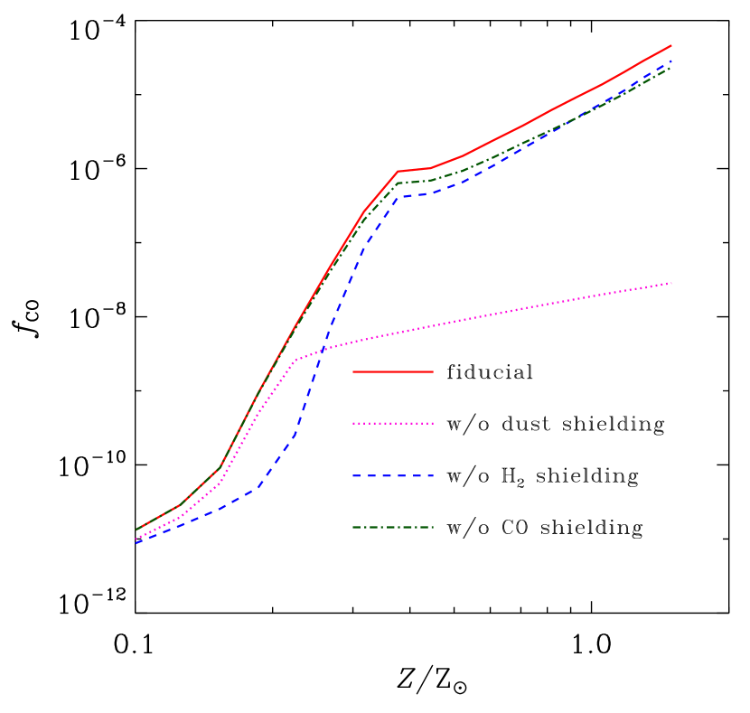
Figure 7: Evolution of the CO fraction, $f_{\mathrm{CO}}$, as a function of metallicity in a typical cloud with the fiducial parameter set. The solid line shows the resulting relation with all the shielding taken into account, and the dotted, dashed, and dot–dashed lines present the relations without shielding by dust, H₂, and CO, respectively.

We observe in Fig. 7 that dust shielding has the largest impact on $f_{\mathrm{CO}}$, especially at high metallicity. Therefore, correctly modelling the dust properties, including the grain size distribution, is essential in estimating $f_{\mathrm{CO}}$ and $X_{\mathrm{CO}}$. The second most important shielding is caused by H₂, which contributes to a factor 2 increase of $f_{\mathrm{CO}}$. The effect of H₂ shielding is almost constant at $Z\gtrsim 0.2$ Z_☉ because the cloud is already fully molecular. CO self-shielding is not negligible at solar metallicity, affecting the CO abundance as much as H₂ shielding.

References

- Accurso et al. (2017) Accurso G., et al., 2017, MNRAS, 470, 4750
- Aniano et al. (2020) Aniano G., et al., 2020, ApJ, 889, 150
- Aoyama et al. (2017) Aoyama S., Hou K.-C., Shimizu I., Hirashita H., Todoroki K., Choi J.-H., Nagamine K., 2017, MNRAS, 466, 105
- Aoyama et al. (2020) Aoyama S., Hirashita H., Nagamine K., 2020, MNRAS, 491, 3844
- Arimoto et al. (1996) Arimoto N., Sofue Y., Tsujimoto T., 1996, PASJ, 48, 275
- Asano et al. (2013a) Asano R. S., Takeuchi T. T., Hirashita H., Inoue A. K., 2013a, Earth, Planets, and Space, 65, 213
- Asano et al. (2013b) Asano R. S., Takeuchi T. T., Hirashita H., Nozawa T., 2013b, MNRAS, 432, 637
- Asplund et al. (2009) Asplund M., Grevesse N., Sauval A. J., Scott P., 2009, ARA&A, 47, 481
- Beitia-Antero et al. (2021) Beitia-Antero L., Gómez de Castro A. I., Vallejo J. C., 2021, ApJ, 908, 112
- Bekki (2013) Bekki K., 2013, MNRAS, 432, 2298
- Bohren & Huffman (1983) Bohren C. F., Huffman D. R., 1983, Absorption and Scattering of Light by Small Particles. Wiley, New York
- Bolatto et al. (2008) Bolatto A. D., Leroy A. K., Rosolowsky E., Walter F., Blitz L., 2008, ApJ, 686, 948
- Bolatto et al. (2013) Bolatto A. D., Wolfire M., Leroy A. K., 2013, ARA&A, 51, 207
- Cazaux & Tielens (2004) Cazaux S., Tielens A. G. G. M., 2004, ApJ, 604, 222
- Chabrier (2003) Chabrier G., 2003, PASP, 115, 763
- Chen et al. (2018) Chen L.-H., Hirashita H., Hou K.-C., Aoyama S., Shimizu I., Nagamine K., 2018, MNRAS, 474, 1545
- Chiang et al. (2021) Chiang I.-D., et al., 2021, ApJ, 907, 29
- Choban et al. (2022) Choban C. R., Kereš D., Hopkins P. F., Sandstrom K. M., Hayward C. C., Faucher-Giguère C.-A., 2022, MNRAS, 514, 4506
- Clark et al. (2016) Clark C. J. R., Schofield S. P., Gomez H. L., Davies J. I., 2016, MNRAS, 459, 1646
- Cormier et al. (2014) Cormier D., et al., 2014, A&A, 564, A121
- Daddi et al. (2010) Daddi E., et al., 2010, ApJ, 713, 686
- De Vis et al. (2021) De Vis P., Maddox S. J., Gomez H. L., Jones A. P., Dunne L., 2021, MNRAS, 505, 3228
- Dohnanyi (1969) Dohnanyi J. S., 1969, J. Geophys. Res., 74, 2531
- Draine (1978) Draine B. T., 1978, ApJS, 36, 595
- Draine & Bertoldi (1996) Draine B. T., Bertoldi F., 1996, ApJ, 468, 269
- Dwek (1998) Dwek E., 1998, ApJ, 501, 643
- Federrath et al. (2008) Federrath C., Klessen R. S., Schmidt W., 2008, ApJ, 688, L79
- Feldmann et al. (2012) Feldmann R., Gnedin N. Y., Kravtsov A. V., 2012, ApJ, 747, 124
- Galli & Palla (1998) Galli D., Palla F., 1998, A&A, 335, 403
- Galliano et al. (2021) Galliano F., et al., 2021, A&A, 649, A18
- Genzel et al. (2012) Genzel R., et al., 2012, ApJ, 746, 69
- Glover & Clark (2016) Glover S. C. O., Clark P. C., 2016, MNRAS, 456, 3596
- Glover & Mac Low (2011) Glover S. C. O., Mac Low M.-M., 2011, MNRAS, 412, 337
- Gould & Salpeter (1963) Gould R. J., Salpeter E. E., 1963, ApJ, 138, 393
- Habing (1968) Habing H. J., 1968, Bull. Astron. Inst. Netherlands, 19, 421
- Hirashita (2015) Hirashita H., 2015, MNRAS, 447, 2937
- Hirashita (2023) Hirashita H., 2023, MNRAS, 518, 3827
- Hirashita & Aoyama (2019) Hirashita H., Aoyama S., 2019, MNRAS, 482, 2555
- Hirashita & Ferrara (2002) Hirashita H., Ferrara A., 2002, MNRAS, 337, 921
- Hirashita & Ferrara (2005) Hirashita H., Ferrara A., 2005, MNRAS, 356, 1529
- Hirashita & Harada (2017) Hirashita H., Harada N., 2017, MNRAS, 467, 699
- Hirashita & Murga (2020) Hirashita H., Murga M. S., 2020, MNRAS, 492, 3779
- Hirata & Padmanabhan (2006) Hirata C. M., Padmanabhan N., 2006, MNRAS, 372, 1175
- Hollenbach & McKee (1979) Hollenbach D., McKee C. F., 1979, ApJS, 41, 555
- Hopkins & Lee (2016) Hopkins P. F., Lee H., 2016, MNRAS, 456, 4174
- Hou et al. (2017) Hou K.-C., Hirashita H., Nagamine K., Aoyama S., Shimizu I., 2017, MNRAS, 469, 870
- Hu et al. (2021) Hu C.-Y., Sternberg A., van Dishoeck E. F., 2021, ApJ, 920, 44
- Hu et al. (2023) Hu C.-Y., Sternberg A., van Dishoeck E. F., 2023, arXiv e-prints, p. arXiv:2301.05247
- Hunt et al. (2015) Hunt L. K., et al., 2015, A&A, 583, A114
- Israel (1997) Israel F. P., 1997, A&A, 328, 471
- Issa et al. (1990) Issa M. R., MacLaren I., Wolfendale A. W., 1990, A&A, 236, 237
- Jones et al. (1996) Jones A. P., Tielens A. G. G. M., Hollenbach D. J., 1996, ApJ, 469, 740
- Kennicutt (1998) Kennicutt Jr. R. C., 1998, ApJ, 498, 541
- Kirchschlager et al. (2022) Kirchschlager F., Mattsson L., Gent F. A., 2022, MNRAS, 509, 3218
- Kobayashi & Tanaka (2010) Kobayashi H., Tanaka H., 2010, Icarus, 206, 735
- Krumholz et al. (2008) Krumholz M. R., McKee C. F., Tumlinson J., 2008, ApJ, 689, 865
- Krumholz et al. (2009) Krumholz M. R., McKee C. F., Tumlinson J., 2009, ApJ, 693, 216
- Lee et al. (1996) Lee H.-H., Herbst E., Pineau des Forets G., Roueff E., Le Bourlot J., 1996, A&A, 311, 690
- Lee et al. (2017) Lee H., Hopkins P. F., Squire J., 2017, MNRAS, 469, 3532
- Leroy et al. (2011) Leroy A. K., et al., 2011, ApJ, 737, 12
- Li et al. (2021) Li Q., Narayanan D., Torrey P., Davé R., Vogelsberger M., 2021, MNRAS, 507, 548
- Lisenfeld & Ferrara (1998) Lisenfeld U., Ferrara A., 1998, ApJ, 496, 145
- Madden et al. (1997) Madden S. C., Poglitsch A., Geis N., Stacey G. J., Townes C. H., 1997, ApJ, 483, 200
- Magdis et al. (2011) Magdis G. E., et al., 2011, ApJ, 740, L15
- Magnelli et al. (2012) Magnelli B., et al., 2012, A&A, 548, A22
- Maloney & Black (1988) Maloney P., Black J. H., 1988, ApJ, 325, 389
- Mathis et al. (1977) Mathis J. S., Rumpl W., Nordsieck K. H., 1977, ApJ, 217, 425
- Mattsson (2016) Mattsson L., 2016, Planet. Space Sci., 133, 107
- McKinnon et al. (2018) McKinnon R., Vogelsberger M., Torrey P., Marinacci F., Kannan R., 2018, MNRAS, 478, 2851
- Moseley et al. (2023) Moseley E. R., Teyssier R., Draine B. T., 2023, MNRAS, 518, 2825
- Narayanan et al. (2011) Narayanan D., Krumholz M., Ostriker E. C., Hernquist L., 2011, MNRAS, 418, 664
- Narayanan et al. (2012) Narayanan D., Krumholz M. R., Ostriker E. C., Hernquist L., 2012, MNRAS, 421, 3127
- Nozawa et al. (2015) Nozawa T., Asano R. S., Hirashita H., Takeuchi T. T., 2015, MNRAS, 447, L16
- Osman et al. (2020) Osman O., Bekki K., Cortese L., 2020, MNRAS, 497, 2002
- Papadopoulos et al. (2012) Papadopoulos P. P., van der Werf P., Xilouris E., Isaak K. G., Gao Y., 2012, ApJ, 751, 10
- Priestley et al. (2021) Priestley F. D., Chawner H., Matsuura M., De Looze I., Barlow M. J., Gomez H. L., 2021, MNRAS, 500, 2543
- Rémy-Ruyer et al. (2014) Rémy-Ruyer A., et al., 2014, A&A, 563, A31
- Romano et al. (2022a) Romano L. E. C., Nagamine K., Hirashita H., 2022a, MNRAS, 514, 1441
- Romano et al. (2022b) Romano L. E. C., Nagamine K., Hirashita H., 2022b, MNRAS, 514, 1461
- Sandstrom et al. (2013) Sandstrom K. M., et al., 2013, ApJ, 777, 5
- Schmidt & Boller (1993) Schmidt K. H., Boller T., 1993, Astronomische Nachrichten, 314, 361
- Schruba et al. (2012) Schruba A., et al., 2012, AJ, 143, 138
- Shetty et al. (2011) Shetty R., Glover S. C., Dullemond C. P., Ostriker E. C., Harris A. I., Klessen R. S., 2011, MNRAS, 415, 3253
- Shi et al. (2016) Shi Y., Wang J., Zhang Z.-Y., Gao Y., Hao C.-N., Xia X.-Y., Gu Q., 2016, Nature Communications, 7, 13789
- Solomon et al. (1987) Solomon P. M., Rivolo A. R., Barrett J., Yahil A., 1987, ApJ, 319, 730
- Spitzer (1978) Spitzer L., 1978, Physical Processes in the Interstellar Medium. Wiley, New York
- Tacconi et al. (2008) Tacconi L. J., et al., 2008, ApJ, 680, 246
- Tanaka et al. (1996) Tanaka H., Inaba S., Nakazawa K., 1996, Icarus, 123, 450
- Tielens (2005) Tielens A. G. G. M., 2005, The Physics and Chemistry of the Interstellar Medium. Cambridge University Press, Cambridge
- Városi & Dwek (1999) Városi F., Dwek E., 1999, ApJ, 523, 265
- Vazquez-Semadeni (1994) Vazquez-Semadeni E., 1994, ApJ, 423, 681
- Weingartner & Draine (2001) Weingartner J. C., Draine B. T., 2001, ApJ, 548, 296
- Wild et al. (1992) Wild W., Harris A. I., Eckart A., Genzel R., Graf U. U., Jackson J. M., Russell A. P. G., Stutzki J., 1992, A&A, 265, 447
- Wilson (1995) Wilson C. D., 1995, ApJ, 448, L97
- Wolfire et al. (2010) Wolfire M. G., Hollenbach D., McKee C. F., 2010, ApJ, 716, 1191
- Yamasawa et al. (2011) Yamasawa D., Habe A., Kozasa T., Nozawa T., Hirashita H., Umeda H., Nomoto K., 2011, ApJ, 735, 44
- Yan et al. (2004) Yan H., Lazarian A., Draine B. T., 2004, ApJ, 616, 895
- Zhu et al. (2003) Zhu M., Seaquist E. R., Kuno N., 2003, ApJ, 588, 243
- Zubko et al. (1996) Zubko V. G., Mennella V., Colangeli L., Bussoletti E., 1996, MNRAS, 282, 1321