Stabilizer entropy dynamics after a quantum quench

Abstract

Stabilizer entropies (SE) measure deviations from stabilizer resources and as such are a fundamental ingredient for quantum advantage. In particular, the interplay of SE and entanglement is at the root of the complexity of classically simulating quantum many-body systems. In this paper, we study the dynamics of SE in a quantum many-body system away from the equilibrium after a quantum quench in an integrable system. We obtain two main results: (i) we show that SE, despite being an $L$-extensive quantity, equilibrates in a time that scales at most linearly with the subsystem size; and (ii) we show that there is a SE length increasing linearly in time, akin to correlations and entanglement spreading.

I Introduction

In the past few decades, significant progress in quantum information science has been closely linked to efforts to synthesize artificial many-body systems. These devices can be used to simulate the quantum dynamics of large systems and execute algorithms with a potentially exponential advantage over classical computersDeutsch and Jozsa (1992); Shor (1994); Lloyd (1996); Grover (1996); Kitaev (1997); Abrams and Lloyd (1999); Harrow et al. (2009). Benchmarking the effectiveness of these devices as quantum systems, in other words, understanding their quantumness, involves identifying the resources that hinder its classical simulation. Entanglement has been viewed as the necessary ingredient for quantumness Aspect et al. (1981, 1982a, 1982b) since the discovery of the Bell inequalities and the first experimental demonstrations Bell (1964); Fine (1982); Terhal (2000); Werner and Wolf (2001) and it plays a fundamental role in the hardness of simulating of quantum many-body systems, e.g. in Tensor Networks Latorre et al. (2004); Orús (2014).

Beyond entanglement, however, resources outside the stabilizer formalismGottesman (1998) are also necessary for complex behavior in quantum many-body systemsBravyi and Kitaev (2005); Campbell and Browne (2010); Campbell and Howard (2017); Howard and Campbell (2017); Seddon and Campbell (2019); Leone et al. (2022a, 2023a); Chamon et al. (2014); Yang et al. (2017); Zhou et al. (2020); Liu and Winter (2022); White et al. (2021); Sewell and White (2022); Koukoulekidis and Jennings (2022); Hinsche et al. (2022). Recently, stabilizer entropy (SE) Leone et al. (2022a) has emerged as a measure of nonstabilizerness in quantum systems. Being an entropy, the SE can be moved around subsystems, with the effect of purifying those from nonstabilizerness, and can give rise to phase transitions as shown Leone et al. (2023b); Niroula et al. (2023). Such quantity can be experimentally measured on a quantum processor Oliviero et al. (2022a); Haug and Kim (2023) and its direct computability makes it amenable for the study of quantum many-body systemsOliviero et al. (2022b); Haug and Piroli (2023a); Lami and Collura (2023); Haug and Piroli (2023b); Tirrito et al. (2023); Odavić et al. (2022); Chen et al. (2022).

The locality of interactions implies that in the gapped ground state of one-dimensional systems, there is a finite correlation length $\xi$ such that the SE is localizedOliviero et al. (2022b); Haug and Piroli (2023a) within a length $L_{0}\sim\xi$, in the sense that SE can be extrapolated by subsystems of size $L$ with an exponentially small error $\mathcal{O}(e^{-L/L_{0}})$. On the other hand, for critical systems $\xi$, is found to diverge resulting in a power law for the approximation error.

In this paper, we investigate the behavior of SE in a quantum many-body system away from equilibrium after the quantum quench of an integrable spin chain. The time profile of SE is computed analytically for all times. The two main results of this paper are (i) SE equilibrates to the value of the infinite time average following a transient period that increases at most linearly with the size of the subsystem, and (ii) the SE length increases ballistically and is upper bounded by a spreading velocity that is proportional to the Lieb-Robinson speed for the systemLieb and Robinson (1972).

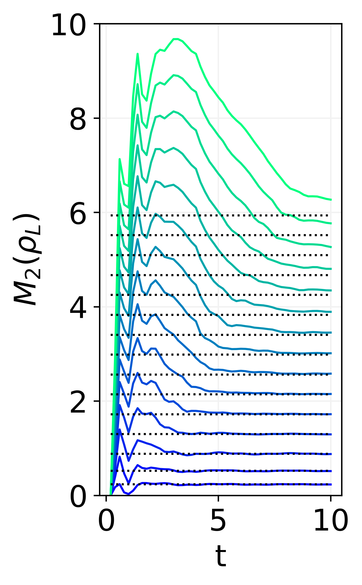
(a)

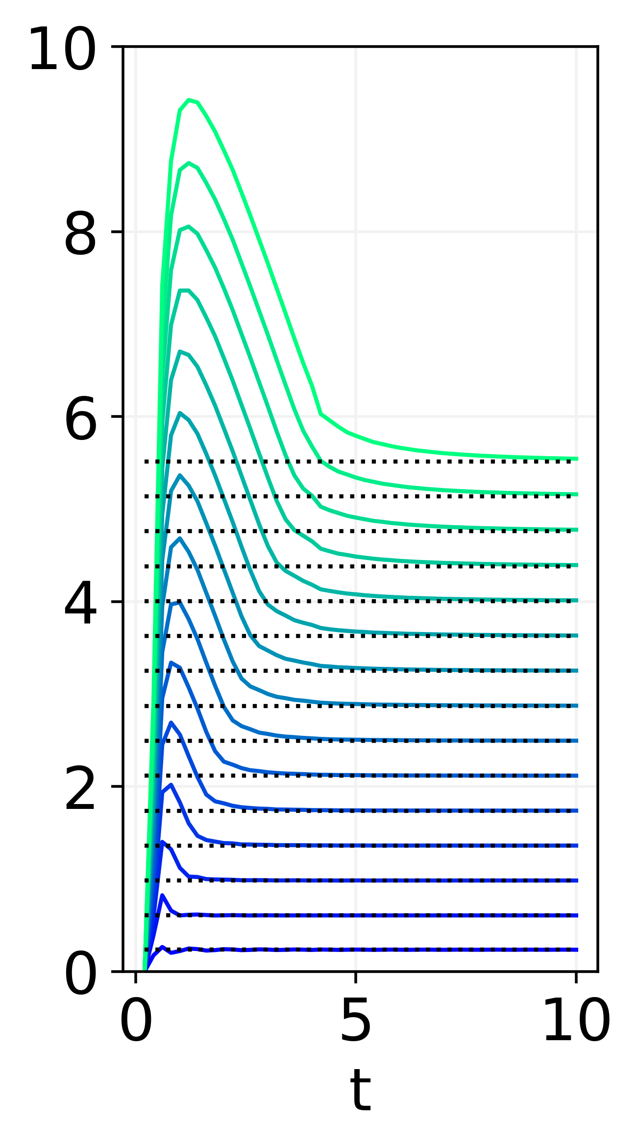
(b)

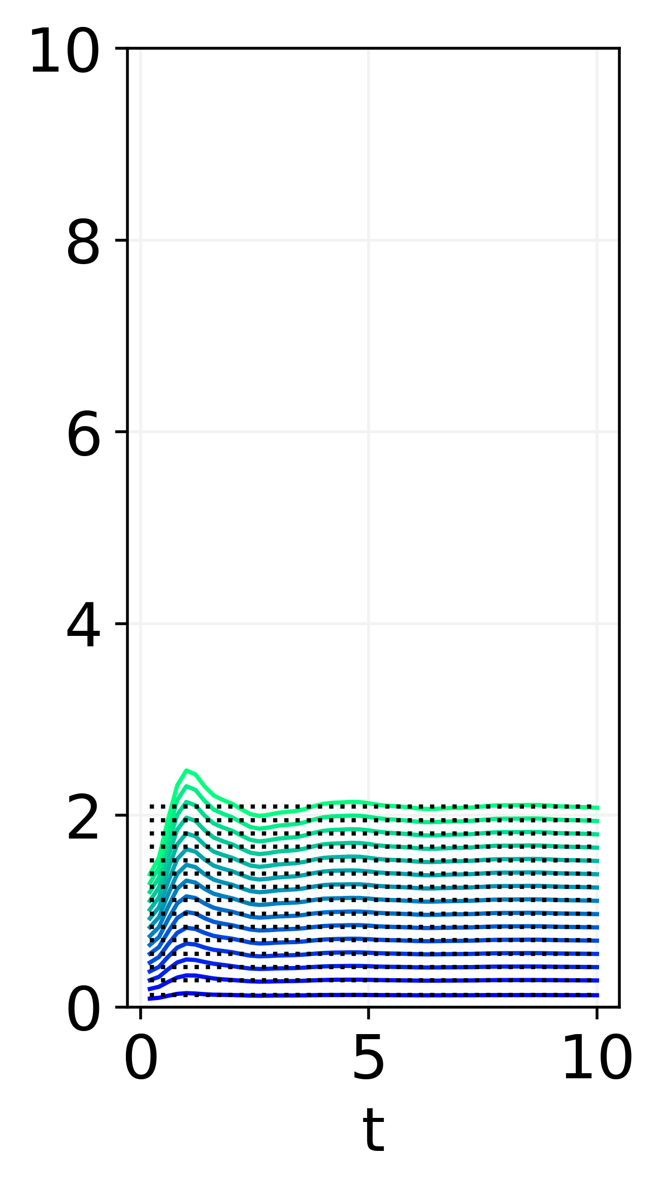
(c)

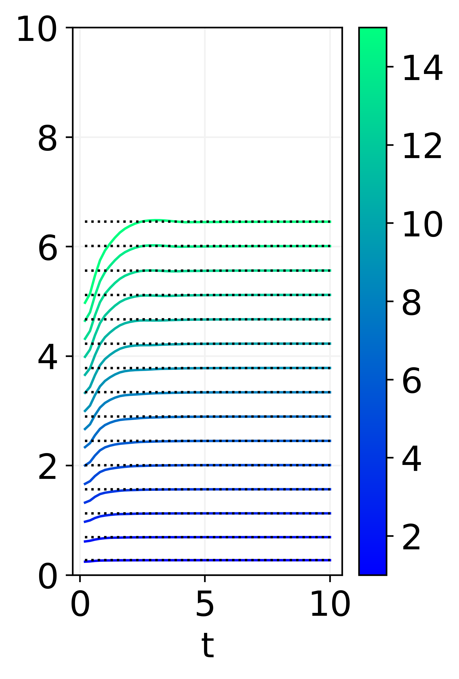
(d)

Figure 1: Solid lines represent the time evolution of the SE $M_{2}$ (in Eq. (1)) of connected subsystems of different sizes $L$, ranging from $1$ (blue lines below) to $15$ (green lines above), after a quench of the transverse field $\lambda$ in the Ising Hamiltonian in Eq. (2). Dotted black lines represent the SE of the corresponding dephased subsystems states $\overline{\psi}_{L}=\operatorname{tr}_{N/L}\lim_{T\to\infty}T^{-1}\int_{0}^{T}\psi_{t}dt$. In Panel (a) for the large quench $\lambda:10^{4}\rightarrow 0.5$; in Panel (b) for the large critical quench $\lambda:10^{4}\rightarrow 1.0$; in Panel (c) for the small quench $\lambda:0.5\rightarrow 0.6$; in Panel (d) for the small critical quench $\lambda:0.9\rightarrow 1.0$. After a time transient, the SE equilibrates to the dephased state value, which is upper-bounded by $L/2$ as expected for an integrable dynamic.

The paper is organized as follows. First, in Section II we introduce the stabilizer entropy (SE) of a subsystem and investigate its evolution in the 1-dimensional transverse field Ising model after a quench. We show that the SE equilibrates to the infinite time average and, after a large quench, the equilibration time of subsystem of size $L$ scales as $L/v_{LR}$, where $v_{LR}$ is the Lieb-Robinson speed associated to the quench. In Section III we introduce the notion of SE length. Looking at its time evolution, we can investigate how non-stabilizerness dynamically delocalizes: first, in Subsection III.1, we use an analytical argument to show that the SE delocalizes in a light-cone, then in Subsection III.2 we show that in the TFIM this length grows ballistically with a speed proportional to the Lieb-Robinson velocity. Finally, Section IV is devoted to conclusions and future perspectives.

II SE away from equilibrium

Let us start with the definition of SELeone et al. (2023a). Let ${\psi}$ be a pure state of a system with $N$ qubits on a chain and $\rho_{L}:=\operatorname{tr}_{N\setminus L}\psi$ its reduced density operator to a subsystem of $L$ contiguous qubits. Denote $\mathcal{P}_{L}$ the Pauli group on such a subsystem. The SE (of order two) of $\rho_{L}$ is defined as

$$M_{2}(\rho_{L}):=-\log_{2}W(\rho_{L})-S_{2}(\rho_{L})$$ (1)

where $W(\rho_{L}):=2^{-L}\sum_{P\in\mathcal{P}_{L}}\operatorname{tr}[(P\rho_{L})^{4}]$ is the so-called stabilizer purity of $\rho_{L}$, while $S_{2}=-\log\operatorname{Pur}(\rho_{L})$ is $2$-Rényi entanglement entropy of $\rho_{L}$ and $\operatorname{Pur}(\rho_{L})\equiv\operatorname{tr}(\rho_{L}^{2})$. SE is a good measure of nonstabilizerness from the point of view of resource theory. Indeed, it has the following properties: (i) faithfulness $M_{\alpha}\left(|\psi\rangle\right)=0$ iff $|\psi\rangle\in\rm{STAB}$, otherwise $M_{\alpha}(|\psi\rangle)>0$, (ii) stability under Clifford operations: $\forall\,\Gamma\in\mathcal{C}_{n}$ we have that $M_{\alpha}\left(\Gamma|\psi\rangle\right)=M_{\alpha}\left(|\psi\rangle\right)$ and (iii) additivity $M_{\alpha}\left(|\psi\rangle\otimes|\phi\rangle\right)=M_{\alpha}\left(|\psi\rangle\right)+M_{\alpha}\left(|\phi\rangle\right)$ (the proof can be found in Leone et al. (2023a)). However, the SE with Rényi index $0<\alpha<2$ are shown to be non-monotone under measurements followed by conditioned Clifford transformations, see Haug and Piroli (2023b).

Let us now turn our attention to the paradigmatic example of a family of $1$-parameter Hamiltonians: the $1$-dimensional transverse-field Ising model (TFIM) $H_{I}(\lambda)$ defined as

$$H_{I}(\lambda)=-\sum_{n}\left(\sigma_{n}^{x}\sigma_{n+1}^{x}+\lambda\sigma_{n}^{z}\right)$$ (2)

with periodic boundary conditions $\sigma_{N+1}:=\sigma_{1}$. In Eq. (2) $\sigma_{i}^{\alpha}$ for $\alpha=x,y,z$ are Pauli matrices acting on the $i$-th spin and $\lambda$ is the strength of the transverse field. The model is integrable for any value of $\lambda$ using the Jordan-Wigner transformation and the Wick theorem Lieb et al. (1961); Pfeuty (1970); Barouch and McCoy (1971). Denote $\ket{\psi_{0}(\lambda)}$ the ground state of $H(\lambda)$. To study the dynamics of SE we subject the system to a quantum quench $H_{I}(\lambda)\mapsto H_{I}(\lambda^{\prime})$ and let $\ket{\psi_{0}(\lambda)}$ evolve under the unitary evolution generated by $H(\lambda^{\prime})$

$$\ket{\psi_{0}(\lambda)}\mapsto\ket{\psi_{t}(\lambda,\lambda^{\prime})}=e^{-iH(\lambda^{\prime})t}\ket{\psi_{0}(\lambda)}$$ (3)

Thanks to Wick’s theorem, the time-dependent expectation values $P_{t}\equiv\operatorname{tr}[P\psi_{t}(\lambda,\lambda^{\prime})]$ can be computed analytically for any subsystem of length $L$ in the thermodynamic limit $N\to\infty$ Mbeng et al. (2020). However, since there are $4^{N}$ such expectation values, we evaluate them for subsystems of sizes $L=1,\ldots,16$.

In Fig.1 we show the evolution of the SE of subsystems under different quenches $H(\lambda^{\prime})$, and the SE $M_{2}(\overline{\rho}_{L})$ of the dephased state $\overline{\rho}_{L}\equiv\operatorname{tr}_{N/L}\sum_{k}\Pi_{k}(\lambda^{\prime})\psi_{0}(\lambda)\Pi_{k}(\lambda^{\prime})=\operatorname{tr}_{N/L}\lim_{T\to\infty}T^{-1}\int_{0}^{T}\psi_{t}dt$. This is the infinite time average of the state, corresponding to the completely dephased state in the basis $\{\Pi_{k}(\lambda^{\prime})\}$ of the Hamiltonian $H_{I}(\lambda^{\prime})$Rigol et al. (2008); Eisert et al. (2015). The initial state is chosen to be the completely polarized state for $\lambda\gg 1$, which is a stabilizer state so that $M_{2}(t=0)=0$. As we can see, there is a transient in which $M_{2}(t)$ increases rapidly before equilibrating to the SE of the dephased state. The equilibration is noteworthy because $M_{2}$ is an $L$-extensive quantity so it is not assured to equilibrate at finite $t$ for every size $L$ under general conditionsTasaki (1998); Reimann (2008); Linden et al. (2009).

For each configuration, the equilibration time $\tau$ can be defined as the time it takes for the subsystem’s SE to reach the SE of the dephased state with fixed tolerance. The scaling of $\tau$ as a function of the system size is depicted in Figure 2 for different quenches. Here we can see that, after a large quench, the equilibration time can be computed as $\tau\simeq L/v$ with $v\propto v_{LR}$, the Lieb-Robinson speed of propagation of signals reconstructed in Appendix C.

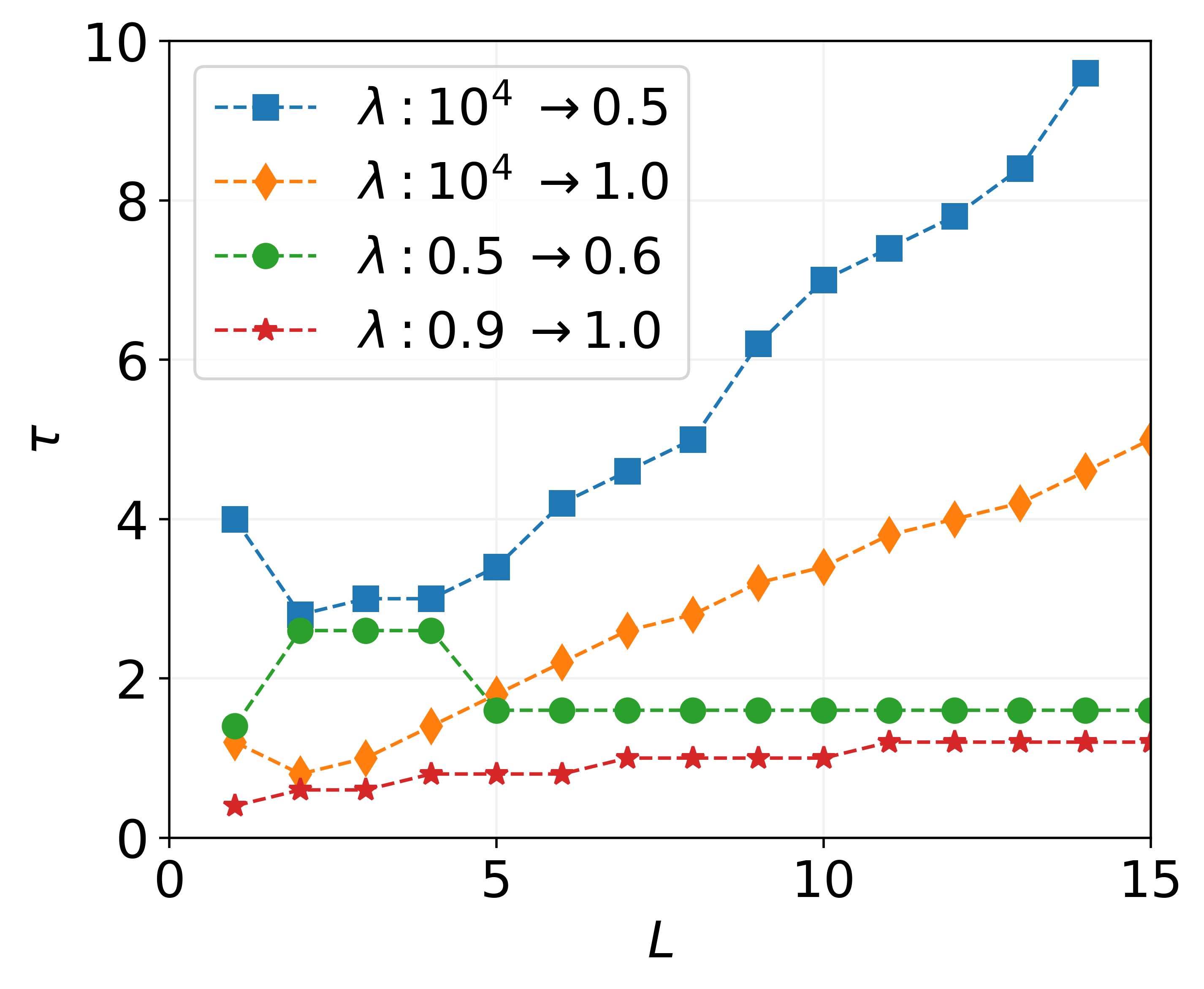
(a)

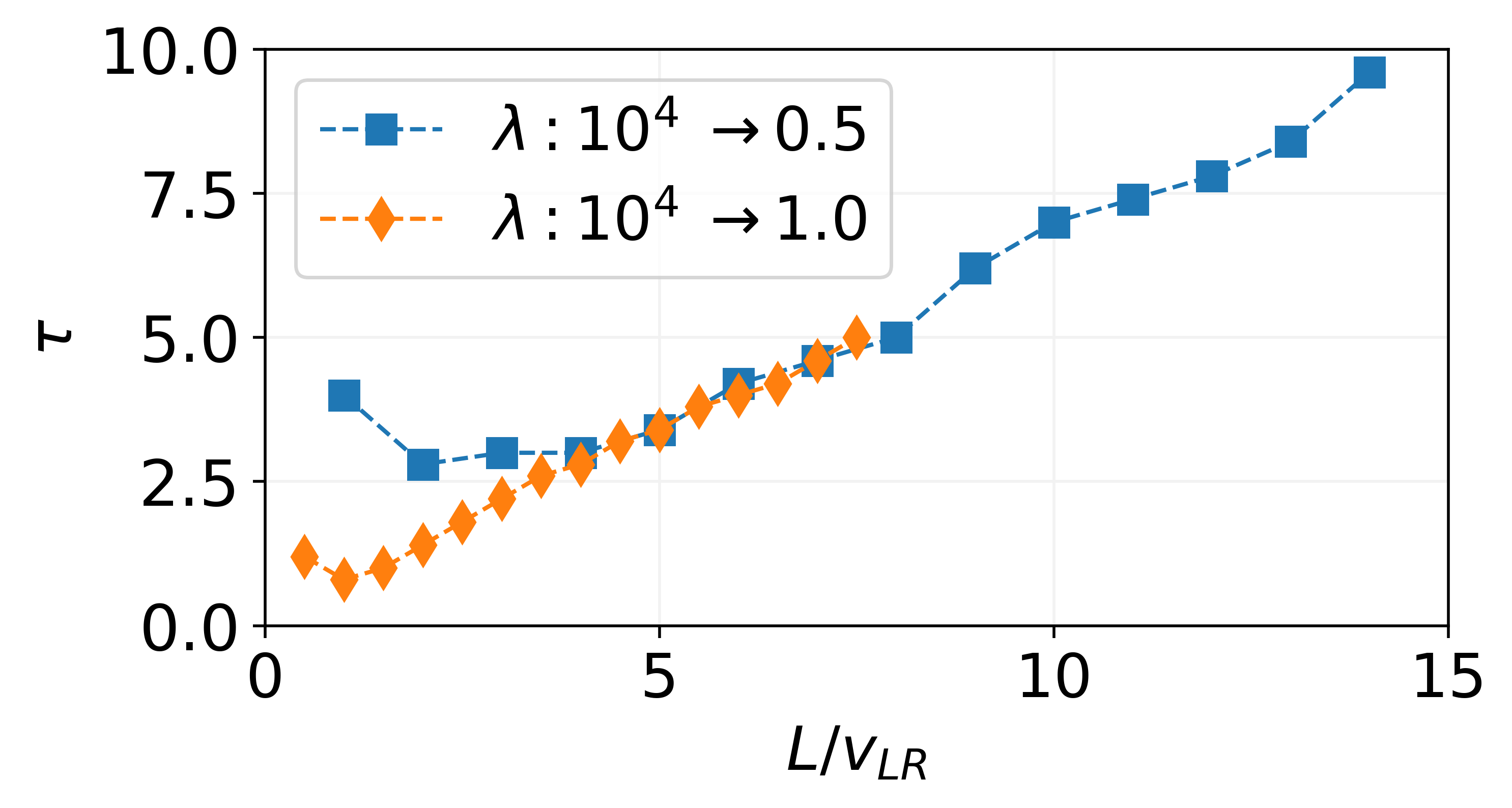
(b)

Figure 2: In Panel (a), the equilibration time ($\tau$) for the subsystem’s SE as a function of the number of sites ($L$) ranging from $0$ to $15$. Here the equilibration time is defined as the time it takes for the subsystem’s SE to reach the SE of the dephased state with a tolerance of $5\%$. We consider four types of quenches: a large non-critical quench (represented by blue squares), a large critical quench (represented by yellow diamonds), a small non-critical quench (represented by green dots), and a small critical quench (represented by red stars). In panel (b) the number of sites is rescaled by the Lieb-Robinson speed. We can see that the equilibration time after a large quench scales as $\tau\simeq L/v$, where $v_{LR}$ is the Lieb-Robinson speed of signals associated with the quench Hamiltonian and $v\propto v_{LR}$.

III SE length dynamics

The localization of SE in a quantum many-body system is described by the SE length. Localization of SE makes this quantity more amenable to computation in large systems. Indeed, although its computation does not involve a minimization procedureCampbell and Browne (2010); Campbell et al. (2017); Seddon and Campbell (2019), it is still exponentially expensive as the number of Pauli operators $P$ is $4^{N}$, as we have seen in the previous section.

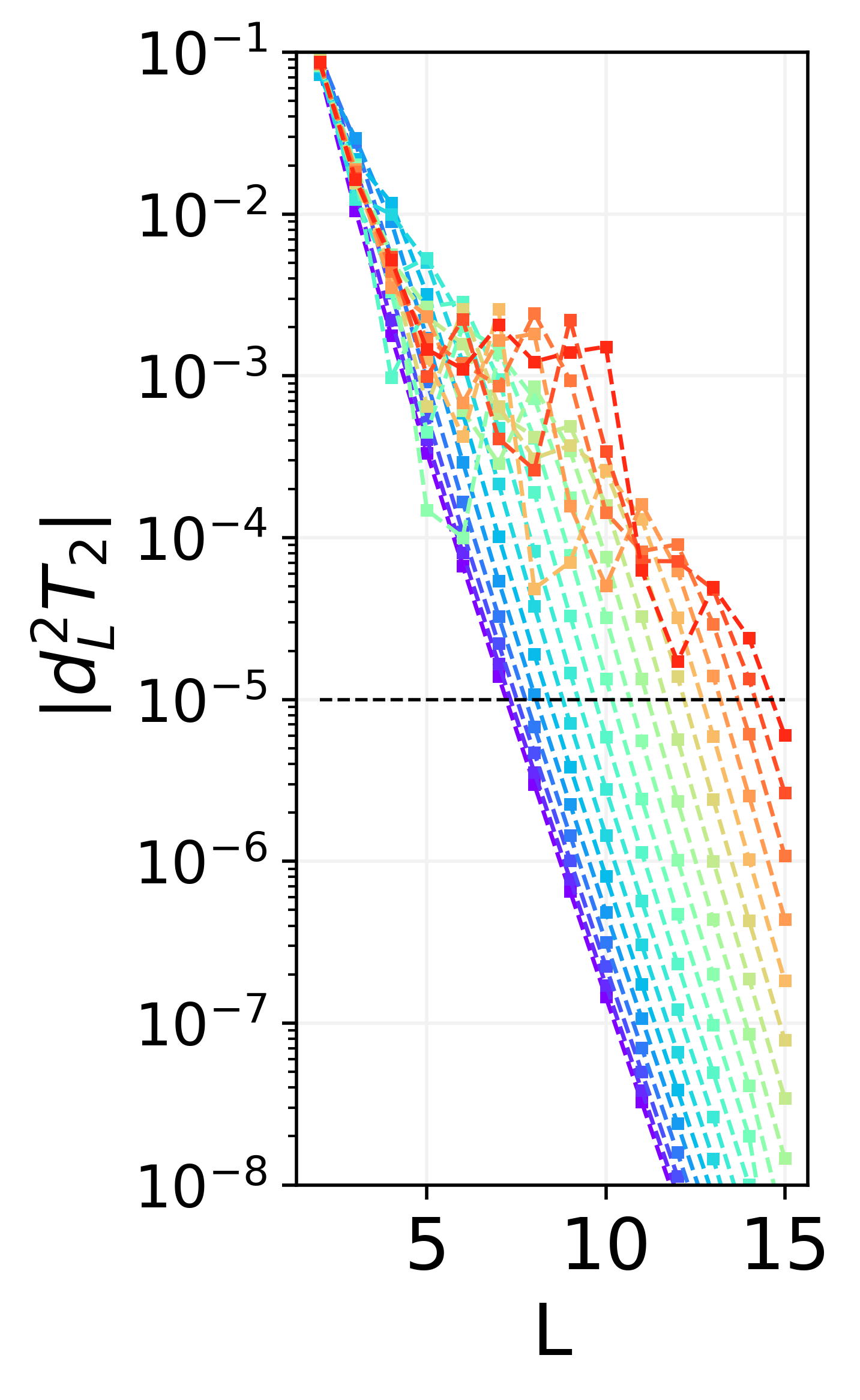
(a)

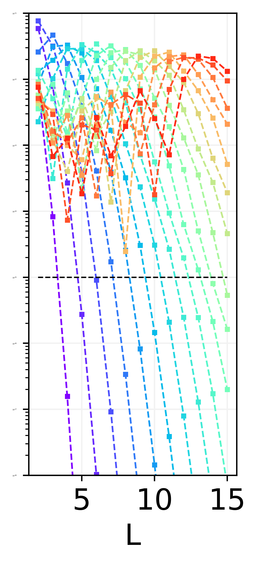
(b)

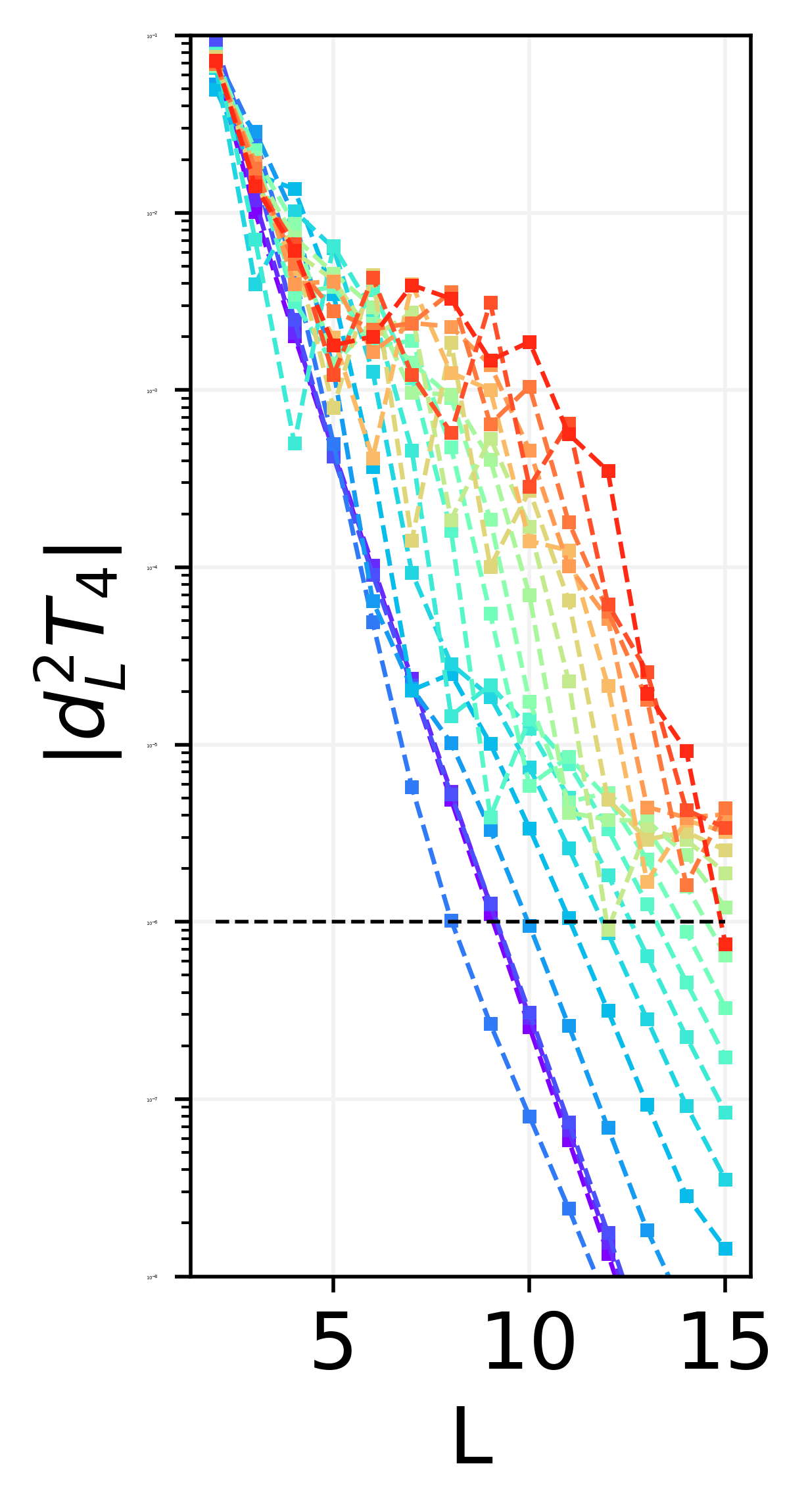
(c)

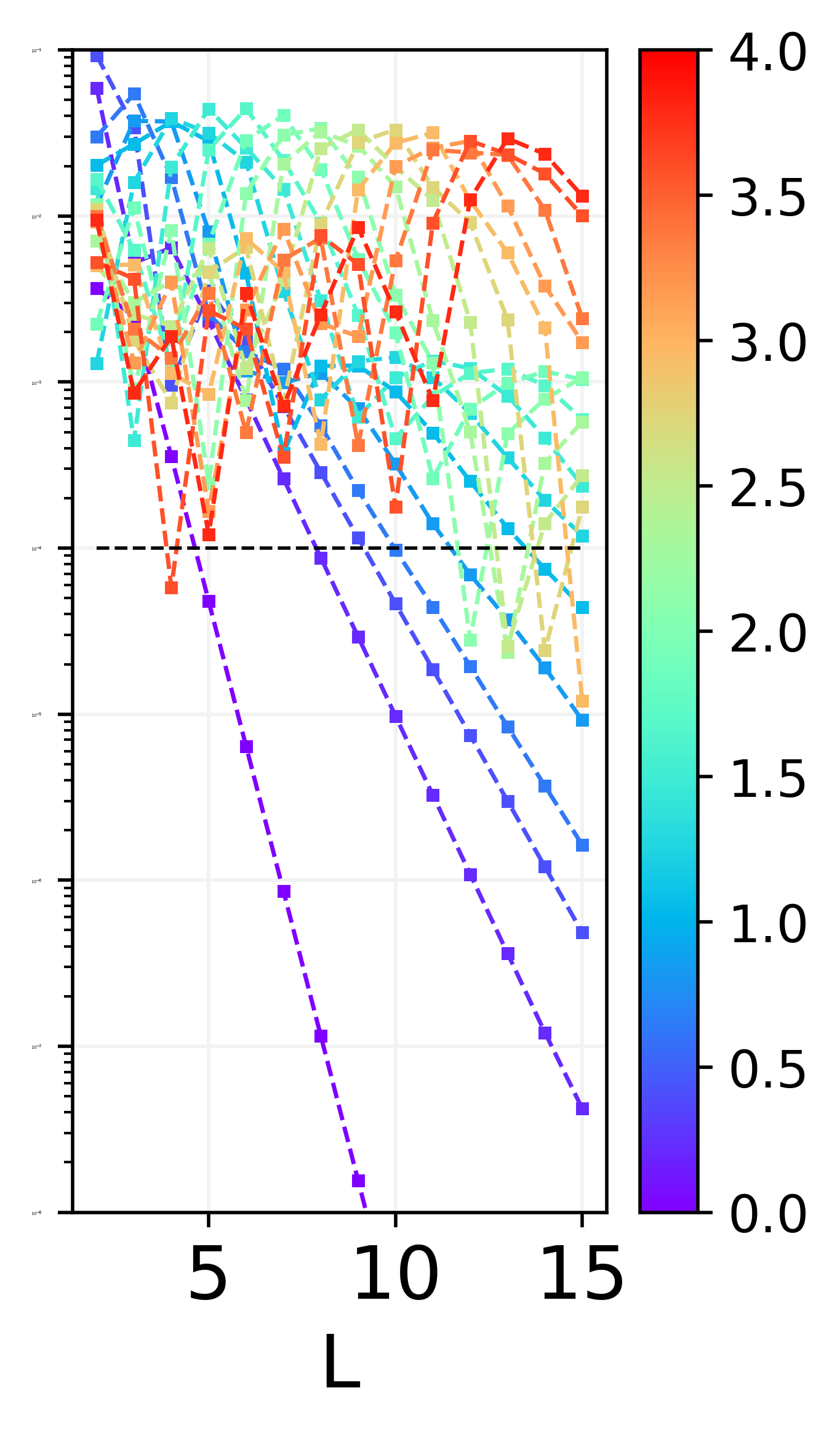
(d)

Figure 3: Second space derivative of $T_{2}(\rho_{L})$ and $T_{4}(\rho_{L})$ (see Eq. (7)) as a function of the subsystem size $L$, ranging from $2$ to $15$, after the quench. Different lines represent different times in the range from $0$ (purple line below) to $4$ (red line above). The horizontal black line represents the error tolerance such that functions above the line decay exponentially. In Panel (a) second derivative of $T_{2}$ for the small quench $\lambda:0.5\rightarrow 0.6$. In Panel (b) second derivative of $T_{2}$ for the large critical quench $\lambda:10^{4}\rightarrow 1.0$. In Panel (c) second derivative of $T_{4}$ for the small quench $\lambda:0.5\rightarrow 0.6$. In Panel (d) second derivative of $T_{4}$ for the large critical quench $\lambda:10^{4}\rightarrow 1.0$. All these derivatives can be upper-bounded by exponentially decaying functions: the SE additivity in Eq. (4) is preserved in time evolution with an exponentially small error for sufficient large subsystems.

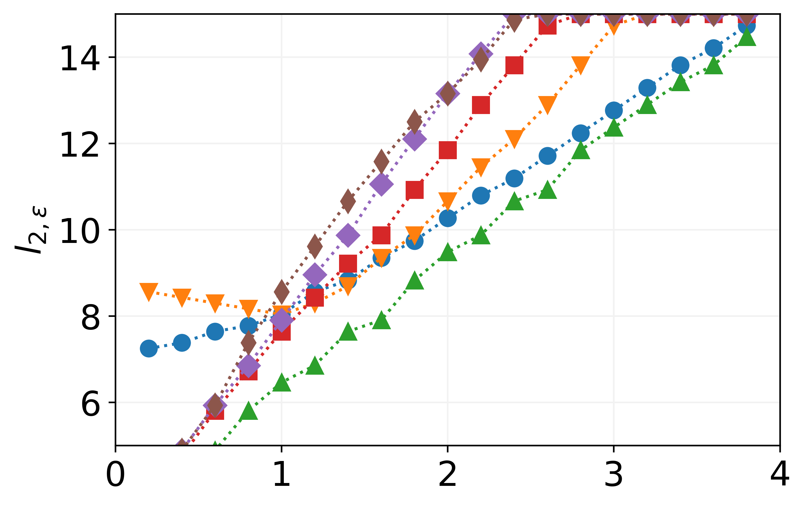
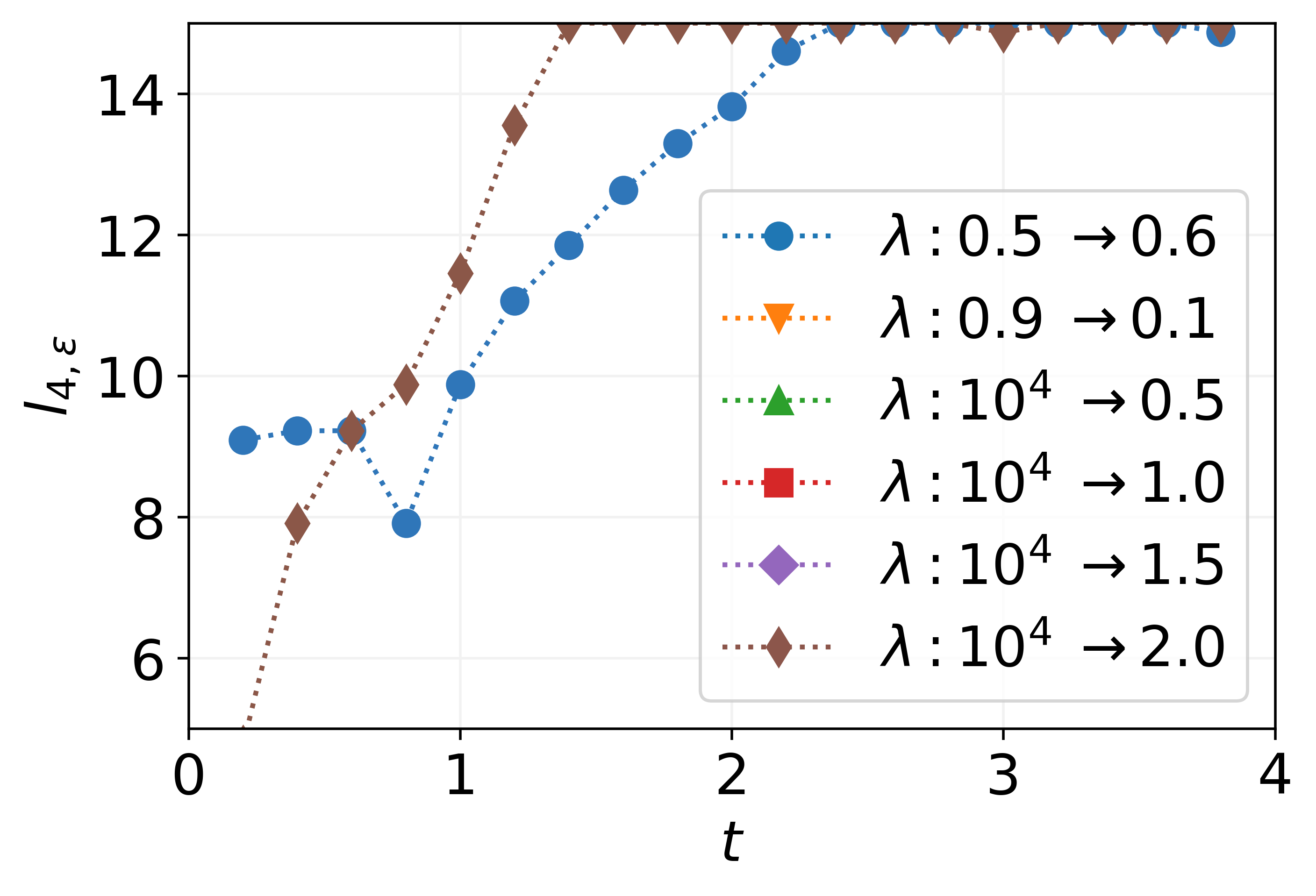
Figure 4: Evolution of the localization lengths $l_{2,\epsilon}$ and $l_{4,\epsilon}$ such that $\lvert\partial_{L}^{2}T_{2}\rvert\leq\epsilon$, $\lvert\partial_{L}^{2}T_{4}\rvert\leq\epsilon$, for different quench protocols and time ranging from $0$ to $4$. We consider large quenches from $\lambda\gg 1$ and small quenches $\lambda^{\prime}=\lambda+0.1$. Quenches to $\lambda=1.0$ are critical. The spreading is ballistic and defines a light-cone.

Recently, there has been an intensive effort for the characterization of systems for which SE can be computed efficiently Oliviero et al. (2022b); Haug and Piroli (2023a); Lami and Collura (2023); Haug and Piroli (2023b). In particular, for translationally invariant ground states of geometrically (gapped) local Hamiltonians Oliviero et al. (2022b), which can be well-described by Matrix Product States (MPSs), and in general for any MPS Haug and Piroli (2023a), there exists a constant $L_{0}$, the SE length, such that for any $L>L_{0}$

$$M_{2}(\rho_{L})\simeq\alpha L+\beta$$ (4)

up to a small additive error $\epsilon\ll\alpha L+\beta$. In Eq. (4) $\alpha,\beta,$ are constants that depend on the whole system state $\ket{\psi}$ Oliviero et al. (2022b) and therefore independent of the subsystem size $L$. The linearity of the SE is a consequence of the finite correlation length of the stateHastings and Koma (2006). More precisely (see Section I of the Supplemental Material) the correction $\epsilon_{L}$ to the linear behavior in Eq. (4) scales as $\epsilon_{L}=\gamma e^{-L/\xi}$, where $\gamma,\xi$ are constants depending on the finitely correlated state under consideration. Such behavior effectively defines the SE length being the constant $L_{0}$ such that $L_{0}=\xi\log\gamma/\epsilon$, for some tolerance $\epsilon\ll\alpha L_{0}+\beta$.

The existence of a (finite) SE length $L_{0}$ makes SE easily computable for extended systems. To see this more concretely, consider a subsystem $X$ of size $L$. From Eq. (4) we see that for $L>L_{0}+1$ and $\Delta\equiv M_{2}(\rho_{L_{0}+1})-M_{2}(\rho_{L_{0}})$ one has

$$M_{2}(\rho_{L})\simeq\Delta(L-L_{0})+M_{2}(\rho_{L_{0}})$$ (5)

which tells us that, once SE is measured for two subsystems of sizes $L_{0}$ and $L_{0}+1$ it can then be efficiently extrapolated, through Eq. (5), to a larger system sizes $L$. Note that it is crucial that $L>L_{0}$ to ensure the validity of Eq. (4) and thus of Eq. (5). The SE length $L_{0}$ quantifies both how non-stabilizerness is localized in the system and the effort needed to compute SE. As an example, in the ground state $\ket{\psi_{0}(\lambda)}$ of the TFIM, the SE length is $L_{0}=1$ for every $\lambda\gg 1$ and $\lambda\ll 1$ Oliviero et al. (2022b).

III.1 Nonstabilizerness delocalization

We have seen that after a quantum quench, $M_{2}$ equilibrates after a time scaling linearly with the size of the system. This suggests that SE is spreading throughout the system. Such spreading should result in an increase in SE length. The main goal of this section is to show that the growth of the SE length $L_{t}$ is upper bounded by an effective light-cone.

We consider the case of states with finite correlation lengths. As it is well known, such states admit an efficient description by MPSOrús (2014). Their time evolution under a local Hamiltonian $H(\lambda^{\prime})$ results in a spreading of correlationsNachtergaele et al. (2006) and increasing entropy of subsystemsEisert (2013). Both effects are encoded in the bond dimensions $D$ for the MPS description, which increases at most as $D(t)\leq e^{A+vt}$Alhambra and Cirac (2021), where $v$ is $O(1)$ in the system size. Using the fact that both the purity $\operatorname{Pur}(\rho_{L})$ and the stabilizer purity $W(\rho_{L})$ can be written as a expectation value of a string of local observables on the replica state $\ket{(\psi\otimes\psi^{*})^{\otimes k}}$ for $k=1,2$ respectively Haug and Piroli (2023a), we can show that the SE length $L_{t}$ obeys the following bound

$$L_{t}\leq L_{0}+v_{s}t\,.$$ (6)

We refer to Section I of the Supplemental Material for details. Here $v_{s}$ is a constant that plays the role of an effective velocity and is $O(1)$ in the system size. The above equation shows that, under the evolution by a local Hamiltonian, SE delocalizes within an effective light-cone constrained by the finite range of interactions in the quench Hamiltonian $H(\lambda^{\prime})$.

III.2 SE length growth in the TFIM

In this subsection, we compute in the concrete case of TFIM the speed $v_{s}$ for the SE length growth, that is, its delocalization. The behavior of the SE length $L_{t}$ is dictated by the correction to the linear scaling in Eq. (4). Recall that Eq. (4) holds up to an additive error $\epsilon_{L_{t}}$, where now $L_{t}$ is a function of time $L_{t}\equiv L_{0}(t)$. The speed at which the error $\epsilon_{L_{t}}$ increases determines the velocity $v_{s}$ of the spreading of $L_{t}$ for $H_{I}(\lambda)$ (see Eq. (6)). We thus numerically investigate the second derivative with respect to $L$ of $M_{2}(\lambda,t)\equiv M_{2}(\rho_{L}^{t}(\lambda))$, for $\rho_{L}^{t}(\lambda)=\operatorname{tr}_{N\setminus L}\ket{\psi_{t}(\lambda)}\!\!\bra{\psi_{t}(\lambda)}$ that, from Eq. (1), is a sum of two terms

$$\partial_{L}^{2}M_{2}(\lambda,t)=\partial_{L}^{2}T_{4}(\lambda,t)-\partial_{L}^{2}T_{2}(\lambda,t)$$ (7)

where $T_{4}(\lambda,t)\equiv-\log W(\rho_{L}^{t}(\lambda))-L$, and $T_{2}(\lambda,t)\equiv S_{2}(\rho_{L}^{t}(\lambda))-L$. Eq. (7) tells us that the behavior of $\epsilon_{L_{t}}$ is, ultimately, determined by the fastest (in $t$) contribution between $\partial_{L}^{2}T_{2}(\lambda,t)$ and $\partial_{L}^{2}T_{4}(\lambda,t)$. Interestingly, the second term $\partial_{L}^{2}T_{2}(\lambda,t)$ encodes the sublinear correction for the area law of MPSs for the $2$-Rényi entropy of entanglement. In other words, the speed at which entanglement spread out in the system can be determined by only the behavior of $\partial_{L}^{2}T_{2}(\lambda,t)$. On the other hand, the corrections to the nonstabilizerness additivity in Eq. (4) and their behavior after the quench are encoded in the evolution of both $\partial_{L}^{2}T_{4}(\lambda,t)$ and $\partial_{L}^{2}T_{2}(\lambda,t)$, which suggests a tight relationship between nonstabilizerness delocalization and entanglement growth. Indeed through theoretical arguments, in Section I of the Supplemental Material, we argue that nonstabilizerness could delocalize two times faster than entanglement. This consideration is found to be true by the numerical analysis below.

To extract the behavior of $L_{t}$ and thus of the velocity $v_{s}$, we fix an error tolerance $\epsilon$ and define $l_{2,\epsilon}(t)$ and $l_{4,\epsilon}(t)$ as solutions of the following inequalities $\lvert\partial_{L}^{2}T_{2}\rvert\leq\epsilon$, $\lvert\partial_{L}^{2}T_{4}\rvert\leq\epsilon$ definitively in time. Then we extract $v_{s}=\max\{v_{T_{2}},v_{T_{4}}\}$ where $v_{T_{k}}\equiv\partial_{t}l_{k,\epsilon}$ for $k=2,4$. In Fig. 3 we depict the behavior of $|\partial_{L}^{2}T_{2}(\lambda,t)|$ and $|\partial_{L}^{2}T_{4}(\lambda,t)|$ for the quench protocols in which the definitive behavior is captured with the computational resources at our disposal, see also see Section II of the Supplemental Material. As expected, we observe that $|\partial_{L}^{2}T_{2}(\lambda,t)|$ and $|\partial_{L}^{2}T_{4}(\lambda,t)|$ decay exponentially below the dotted line representing the chosen error tolerance $\epsilon$. The associated lengths $l_{2,\epsilon}(t)$ and $l_{4,\epsilon}(t)$ as a function of $t$ are shown in Fig. 4 for $t=0,\ldots,4$: after an initial transient, both $l_{2,\epsilon}(t)$ and $l_{4,\epsilon}(t)$ grow ballistically. The associated velocities are: $v_{T2}\approx 2.5$ for $\lambda^{\prime}=0.5$ and $v_{T2}\approx 5$ for $\lambda^{\prime}\in\{1,1.5,2\}$, independently of the initial state; while $v_{T4}\approx 5$ for $\lambda^{\prime}=0.5$ and $v_{T4}\approx 10$ for $\lambda^{\prime}=2.0$. We conclude that, being $v_{T_{4}}>v_{T_{2}}$, $v_{s}\approx v_{T_{4}}$ and thus – compatibly with our theoretical considerations – the SE delocalizes two times faster than entanglement entropy.

Finally, we are going to show that the velocity $v_{s}$ is proportional to the Lieb-Robinson speed $v_{LR}$. The Lieb-Robinson velocity associated with the Ising Hamiltonian can be reconstructed from the revivals after the quench. Revivals are brief detachments from the average value observables, whose magnitude decays in time as the equilibration process nears completion. During these detachments, the system state gets briefly closer to the initial state. Therefore, revivals can be detected by looking at the Loschmidt echo (LE), that is, the squared fidelity between the evolved state and the initial state. The revival times $T_{\text{rev}}$ are proportional to the system size $N$ and are related to maximal group velocity in integrable systems, and therefore to the Lieb-Robinson speed in generic local systems, as $T_{\text{rev}}\approx N/(2v_{\text{LR}})$ Häppölä et al. (2012). The LE can be efficiently calculated for integrable spin chains in the fermionic representation described in Ref. Lieb et al. (1961). In Appendix C we show that, independently of the initial state, Lieb-Robinson speed is $v_{\text{LR}}=2$ for the paramagnetic quench $\lambda^{\prime}>1$, and $v_{\text{LR}}=2\lambda^{\prime}$ for the ferromagnetic quench $\lambda^{\prime}<1$. This result suggests a proportionality relation between $v_{s}$ and $v_{\text{LR}}$.

IV Conclusions

In this work, we studied for the first time the behavior away from equilibrium of the non-stabilizer properties of a quantum many-body system after a sudden quench. The system studied is the integrable quantum Ising chain, which allowed for a thoroughly analytical treatment, and non-stabilizerness is computed through the Stabilizer Rényi Entropy $M_{2}$. Two main results are found: (i) $M_{2}$ increases and finally equilibrates in a time proportional to the system size, and (ii) one can define a stabilizer entropy length $L_{t}$ that describes the SE localization Oliviero et al. (2022b). Such length increases linearly in time showing that $M_{2}$ spreads ballistically through the system until complete delocalization.

In perspective, this work calls for several questions. InLeone et al. (2021a); Oliviero et al. (2021a, 2022c); Leone et al. (2022b, c, 2023b) it has been shown that the onset of quantum chaotic behavior in quantum circuits corresponds to a value of $M_{2}>N/2$, and full-fledged quantum chaos is attained near-maximal values for SE. Of course, chaos in quantum circuits is not the same than chaos in Hamiltonian systems, being defined there as the onset of universal entanglement features or universal behavior of the OTOCsLeone et al. (2021a). However, our results show that the equilibrium value of SE for the integrable quantum quench is below the quantum chaotic threshold of quantum circuits. This fact raises the question whether the equilibrium SE is a tell-tale of the onset of quantum chaos in Hamiltonians system. We indeed speculate that a non-integrable system will equilibrate to a larger value for $M_{2}$. It would be intriguing if the increase in equilibrium SE compared to the integrable case would depend on the strength of the interability breaking term.

Second, preliminary numerical analysis suggests that subtle features of SE dynamics may be erased by the operation of partial trace. This is akin to the problem of presence of thermal fluctuations when evaulating entanglement. A possible strategy would be to localize SE in a subsystem by measurements in a Clifford basis (e.g., the computational basis) and evaluate the local residual SE in the pure state. This would entail to average over all the possible Clifford measurements.

Third, the onset of quantum chaos depends on the interplay between both entanglement and SE, Leone et al. (2021a, 2022c); Oliviero et al. (2021a); Dowling et al. (2023); Leone et al. (2021b); Oliviero et al. (2021b); Leone et al. (2022b); Oliviero et al. (2022c); Dowling and Modi (2023); Omanakuttan et al. (2023); Goto et al. (2022); True and Hamma (2022); Kim et al. (2023) and it is still an open question to what extent they are sufficient and/or necessary. RecentlyTirrito et al. (2023), it has been shown that the flatness of the entanglement spectrum of a subsystem is a good probe for SE. Since it is also a probe for entanglement, it is tempting to study the dynamics of flatness to probe the onset of quantum chaos.

Finally, finite size scaling in $L$ for larger sizes would allow for a reliable analysis of the temporal fluctuations. To this end, we plan to employ Monte-Carlo methods to sample SE efficiently. Finally, we remark on the fascinating relationship between SE and the bond dimension $D$. The study of the interplay of SE with the efficiency of tensor network methods is thus potentially of great importance for the issue of simulating quantum many-body systems on a classical computer.

Appendix A Proof of Eq. (6)

First of all, let us define the functions $T_{4}(\lambda,t)\equiv-\log W(\rho_{L}^{t}(\lambda))-L$, and $T_{2}(\lambda,t)\equiv S_{2}(\rho_{L}^{t}(\lambda))-L$. In terms of $T_{2}$ and $T_{4}$, the SE can be written as

$$M_{2}(\lambda,t)=T_{4}(\lambda,t)-T_{2}(\lambda,t).$$ (8)

As shown in Haug and Piroli (2023a), $2^{T_{2}}$ and $2^{T_{4}}$ are expectation values of strings of $L$ connected observables on replica states. More precisely, define $\ket{\psi^{(k)}}\equiv\ket{(\psi\otimes\psi^{*})^{\otimes k}}$ for $k=1,2$. Define the local observable $A_{i}^{(k)}={\mathchoice{\rm 1\mskip-4.0mul}{\rm 1\mskip-4.0mul}{\rm 1\mskip-4.5mul}{\rm 1\mskip-5.0mul}}_{i}^{\otimes 2k}+\sum_{\alpha=1}^{3}(\sigma_{i}^{\alpha}\otimes\sigma_{i}^{\alpha*})^{\otimes k}$ for $k=1,2$ and $\sigma_{i}^{\alpha}$ for $\alpha=x,y,z$ being single qubit Pauli matrices. Then $2^{T_{2k}}$ for $k=1,2$ can be recast as

$$2^{T_{2k}(\lambda,t)} =\bra{\psi^{(k)}}A^{(k)}_{1}\otimes\dots\otimes A^{(k)}_{L}\otimes{\mathchoice{\rm 1\mskip-4.0mul}{\rm 1\mskip-4.0mul}{\rm 1\mskip-4.5mul}{\rm 1\mskip-5.0mul}}_{N\setminus L}\ket{\psi^{(k)}}.$$ (9)

To explain the behavior of the SE under time evolution and its relation to the locality, we want to understand how strings of observables behave in a state with finite correlation length, and how they change while, after a quantum quench, correlations spread out in the system.

We start by looking at the initial translationally invariant state $\ket{\psi(0)}$. Having a finite correlation length, this can be represented as an MPS with polynomial bond dimension $D$. Similarly, $\ket{\psi^{(k)}}$ for $k=1,2$ is a MPS state with bond dimension $D_{k}=D^{2k}$. Let $\tau_{\psi^{(k)}}$ be the transfer matrix of the MPS and $\tau_{\psi^{(k)}\!,A}$ be the transfer matrix of the MPS contracted with the local operator $A$. The expectation value of a string of local operators $A_{i}^{(k)}$ can be written as:

$$\bra{\psi^{(k)}}A^{(k)}_{1}\otimes\dots\otimes A^{(k)}_{L}\otimes{\mathchoice{\rm 1\mskip-4.0mul}{\rm 1\mskip-4.0mul}{\rm 1\mskip-4.5mul}{\rm 1\mskip-5.0mul}}_{N\setminus L}\ket{\psi^{(k)}}$$

$$=\lim_{N\rightarrow\infty}\operatorname{tr}\left(\tau_{\psi^{(k)}}^{N-L}\tau_{\psi^{(k)}\!,A}^{L}\right)$$ (10)

Now, we call $\ket{R_{\psi^{(k)}}^{(i)}}$ and $\ket{L_{\psi^{(k)}}^{(i)}}$ the right and left eigenvectors of $\tau_{\psi^{(k)}}$ and $\lambda_{\psi^{(k)}}^{(i)}$ the associated eigenvalues. In this way, the transfer matrix can be written as

$$\tau_{\psi^{(k)}}=\sum_{i=1}^{D_{k}^{2}}\lambda_{\psi^{(k)}}^{(i)}\ket{R_{\psi^{(k)}}^{(i)}}\bra{L_{\psi^{(k)}}^{(i)}},$$ (11)

where $\lvert\lambda_{\psi^{(k)}}^{(i)}\rvert>\lvert\lambda_{\psi^{(k)}}^{(i+1)}\rvert$, and $\lambda_{\psi^{(k)}}^{(1)}=1$ for the normalization condition. Analogously, we can write

$$\tau_{\psi^{(k)}\!,A}=\sum_{i=1}^{D_{k}^{2}}\lambda_{\psi^{(k)}\!,A}^{(i)}\ket{R_{\psi^{(k)}\!,A}^{(i)}}\bra{L_{\psi^{(k)}\!,A}^{(i)}},$$ (12)

with $\lvert\lambda_{\psi^{(k)}\!,A}^{(i)}\rvert>\lvert\lambda_{\psi^{(k)}\!,A}^{(i+1)}\rvert$. The eventual degeneration of eigenvalues does not affect the general behavior of this proof. Hence, a string expectation value can be written as

$$\bra{\psi^{(k)}}A^{(k)}_{1}\otimes\dots\otimes A^{(k)}_{L}\otimes{\mathchoice{\rm 1\mskip-4.0mul}{\rm 1\mskip-4.0mul}{\rm 1\mskip-4.5mul}{\rm 1\mskip-5.0mul}}_{N\setminus L}\ket{\psi^{(k)}}$$

$$=\sum_{i=1}^{D_{k}^{2}}\left(\lambda_{\psi^{(k)}\!,A}^{(i)}\right)^{L}\bra{L_{\psi^{(k)}}^{(i)}}R_{\psi^{(k)}\!,A}^{(i)}\rangle\bra{L_{\psi^{(k)}\!,A}^{(i)}}R_{\psi^{(k)}}^{(i)}\rangle.$$ (13)

At this point, we define

$$2^{m(\psi^{(k)})} :=\lambda_{\psi^{(k)}\!,A}^{(1)}$$ (14)

$$2^{q(\psi^{(k)})} :=\bra{L_{\psi^{(k)}}^{(1)}}R_{\psi^{(k)}\!,A}^{(1)}\rangle\bra{L_{\psi^{(k)}\!,A}^{(1)}}R_{\psi^{(k)}}^{(1)}\rangle$$ (15)

$$e^{-1/\xi(\psi^{(k)})} :=\left\lvert\frac{\lambda_{\psi^{(k)}\!,A}^{(2)}}{\lambda_{\psi^{(k)}\!,A}^{(1)}}\right\rvert$$ (16)

$$F(\psi^{(k)}) :=\left\lvert\frac{\bra{L_{\psi^{(k)}}^{(2)}}R_{\psi^{(k)}\!,A}^{(2)}\rangle\bra{L_{\psi^{(k)}\!,A}^{(2)}}R_{\psi^{(k)}}^{(2)}\rangle}{\bra{L_{\psi^{(k)}}^{(1)}}R_{\psi^{(k)}\!,A}^{(1)}\rangle\bra{L_{\psi^{(k)}\!,A}^{(1)}}R_{\psi^{(k)}}^{(1)}\rangle}\right\rvert.$$ (17)

Since $\left\lvert\lambda_{\psi^{(k)}\!,A}^{(i)}\right\rvert^{L}\gg\left\lvert\lambda_{\psi^{(k)}\!,A}^{(i+1)}\right\rvert^{L}$, for sufficiently large $L$ we obtain

$$\bra{\psi^{(k)}}A^{(k)}_{1}\otimes\dots\otimes A^{(k)}_{L}\otimes{\mathchoice{\rm 1\mskip-4.0mul}{\rm 1\mskip-4.0mul}{\rm 1\mskip-4.5mul}{\rm 1\mskip-5.0mul}}_{N\setminus L}\ket{\psi^{(k)}}$$

$$=2^{m(\psi^{(k)})L+q(\psi^{(k)})}(1+\varepsilon^{(k)})$$ (18)

where

$$\lvert\varepsilon^{(k)}\rvert\leq D_{k}^{2}e^{-L/\xi(\psi^{(k)})}F(\psi^{(k)})\ll 1.$$ (19)

It should be noted that the derivation of this bound assumes that $F(\psi^{(k)})$ is finite. In the event that this condition is not met, an equivalent derivation can be obtained by considering the next eigenvalue $\lambda_{\psi^{(k)}\!,A}^{(2)}$. In this case, $F(\psi_{k}):=\left\lvert\bra{L_{\psi^{(k)}}^{(3)}}R_{\psi^{(k)}\!,A}^{(3)}\rangle\bra{L_{\psi^{(k)}\!,A}^{(3)}}R_{\psi^{(k)}}^{(3)}\rangle\right\rvert/$ $\left\lvert\bra{L_{\psi^{(k)}}^{(2)}}R_{\psi^{(k)}\!,A}^{(2)}\rangle\bra{L_{\psi^{(k)}\!,A}^{(2)}}R_{\psi^{(k)}}^{(2)}\rangle\right\rvert$, and the linear approximation is preserved with the same exponential correction.

With this formalism, also the effect of locality on time evolution can be easily addressed. When an MPS evolves with a local Hamiltonian $H(\lambda^{\prime})$, the spreading of correlationsNachtergaele et al. (2006) and the increasing entropy of subsystemsEisert (2013) are encoded in the bond dimensions, which increases at most as $D(t)\leq e^{A+vt}$Alhambra and Cirac (2021), where $v$ is $O(1)$ in the system size. We can then generalize the result obtained in Eq. (A) in the following way

$$\bra{\psi^{(k)}(t)}A^{(k)}_{1}\otimes\dots\otimes A^{(k)}_{L}\otimes{\mathchoice{\rm 1\mskip-4.0mul}{\rm 1\mskip-4.0mul}{\rm 1\mskip-4.5mul}{\rm 1\mskip-5.0mul}}_{N\setminus L}\ket{\psi^{(k)}}$$

$$=2^{m(\psi^{(k)}(t))L+q(\psi^{(k)(t)})}(1+\varepsilon^{(k)})$$ (20)

where we defined $\ket{\psi^{(k)}(t)}\equiv[U_{t}\otimes U_{t}^{*}]^{\otimes k}\ket{\psi^{(k)}}$ with $U_{t}=e^{-iH(\lambda^{\prime})t}$. And consequently $\varepsilon^{(k)}$ is now bounded for sufficiently large $L$ as:

$$\lvert\varepsilon^{(k)}\rvert\leq e^{4kA+4kvt}e^{-L/\xi(\psi^{(k)}(t))}F(\psi^{(k)}(t))\ll 1.$$ (21)

where we used that $D_{k}=D^{2k}$ and consequently that $D_{k}(t)=D(t)^{2k}\leq e^{2kA+2kvt}$. At this point we define $\varepsilon_{0}^{(k)}=e^{4kA}\max_{t}F(\psi(t))$ and $\chi^{(k)}=\max_{t}\xi(\psi^{(k)}(t))$. We obtain that

$$\lvert\varepsilon^{(k)}\rvert\leq\varepsilon_{0}^{(k)}e^{(4kv\chi^{(k)}t-L)/\chi^{(k)}}.$$ (22)

With this result, let us focus on the behavior of the SE $M_{2}=T_{4}-T_{2}$. Since $2^{T_{2}}$ and $2^{T_{4}}$ are equal to

$$T_{2} =m(\psi^{(1)}(t))L+q(\psi^{(1)}(t))+\varepsilon^{(1)}$$

$$T_{4} =m(\psi^{(2)}(t))L+q(\psi^{(2)}(t))+\varepsilon^{(2)}$$

$$\lvert\varepsilon^{(1)}\rvert \leq\varepsilon_{0}^{(1)}e^{(4v\chi^{(1)}t-L)/\chi^{(1)}}$$

$$\lvert\varepsilon^{(2)}\rvert \leq\varepsilon^{(2)}_{0}e^{(8v\chi^{(2)}t-L)/\chi^{(2)}}.$$ (23)

It follows that

$$M_{2}(\rho_{L}) =[m(\psi^{(2)}(t))-m(\psi^{(1)}(t))]L$$

$$+[q(\psi^{(2)}(t))-q(\psi^{(1)}(t))]+\varepsilon_{M}$$

$$\lvert\varepsilon_{M}\rvert \leq 2\max\{\varepsilon^{(1)},\varepsilon^{(2)}\}.$$ (24)

In a nutshell, during time evolution corrections to the linearity of nonstabilizerness are exponentially small out from a light-cone. The speed at which the exponential bound increases determines the light-cone in which the SE spreads out. To figure this out, we fix an error tolerance $\epsilon$ and we find the values $L_{2,\epsilon}$ and $L_{4,\epsilon}$ such that $\lvert\varepsilon^{(1)}\rvert\leq\epsilon$ and $\lvert\varepsilon^{(2)}\rvert\leq\epsilon$ definitively as a consequence of the previous bound. The SE length $L_{t}$ is $\max\{L_{2,\epsilon},L_{4,\epsilon}\}$.

Taking into account Eqs.(A) $L_{2,\epsilon}$ and $L_{2,\epsilon}$ increases at most as:

$$L_{2,\epsilon} =\xi(\psi^{(1)}(t))\log(\varepsilon_{0}^{(1)}/\epsilon)+4v\chi^{(1)}t$$

$$L_{4,\epsilon} =\xi(\psi^{(2)}(t))\log(\varepsilon^{(2)}_{0}/\epsilon)+8v\chi^{(2)}t$$ (25)

Therefore, we can conclude that

$$L_{t}\leq L_{0}+v_{s}t\,,$$ (26)

where $v_{s}=\max\{4v\chi^{(1)},8v\chi^{(2)}\}$ is $O(1)$ in the system size. Remarkably, when $\chi^{(1)}$ is comparable with $\chi^{(2)}$, the error on $T_{4}$ spreads two times faster than the error on $T_{2}$.

Appendix B Additional numerical data

In Figures 5 and 6, we show the exponential decay of the correction to the linear behavior of $T_{2}$, encoded in the second space derivative, after different quenches. Analogously, in Figures 7 and 8 we represent the exponential decay of the correction to the linear behavior of $T_{4}$.

In each figure, we can see that the exponential behavior is definitive for a sufficiently large system, as predicted in Section A. The size of this large system depends on time and on the quench protocol. Therefore, capturing the definitive behavior is not always possible with our computational resources. When the definitive behavior of the derivative is not captured by our data (e.g. 6 panel (b)) the dashed line is red, otherwise it is black. In this latter case, we observe that the derivative decays definitively exponentially below the dotted line.

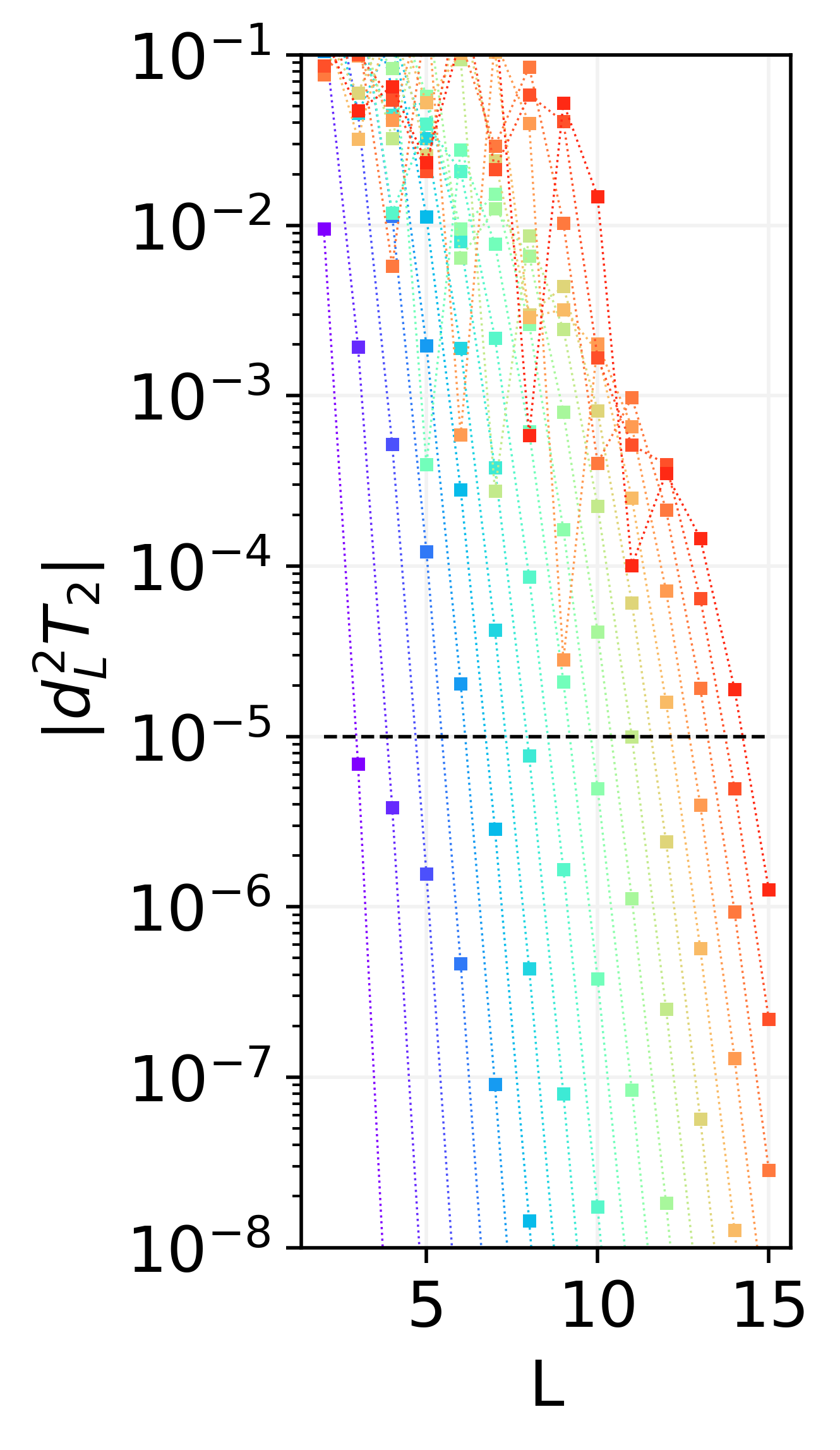
(a)

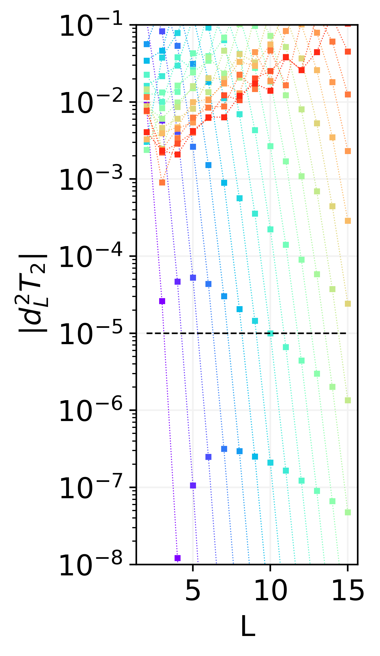
(b)

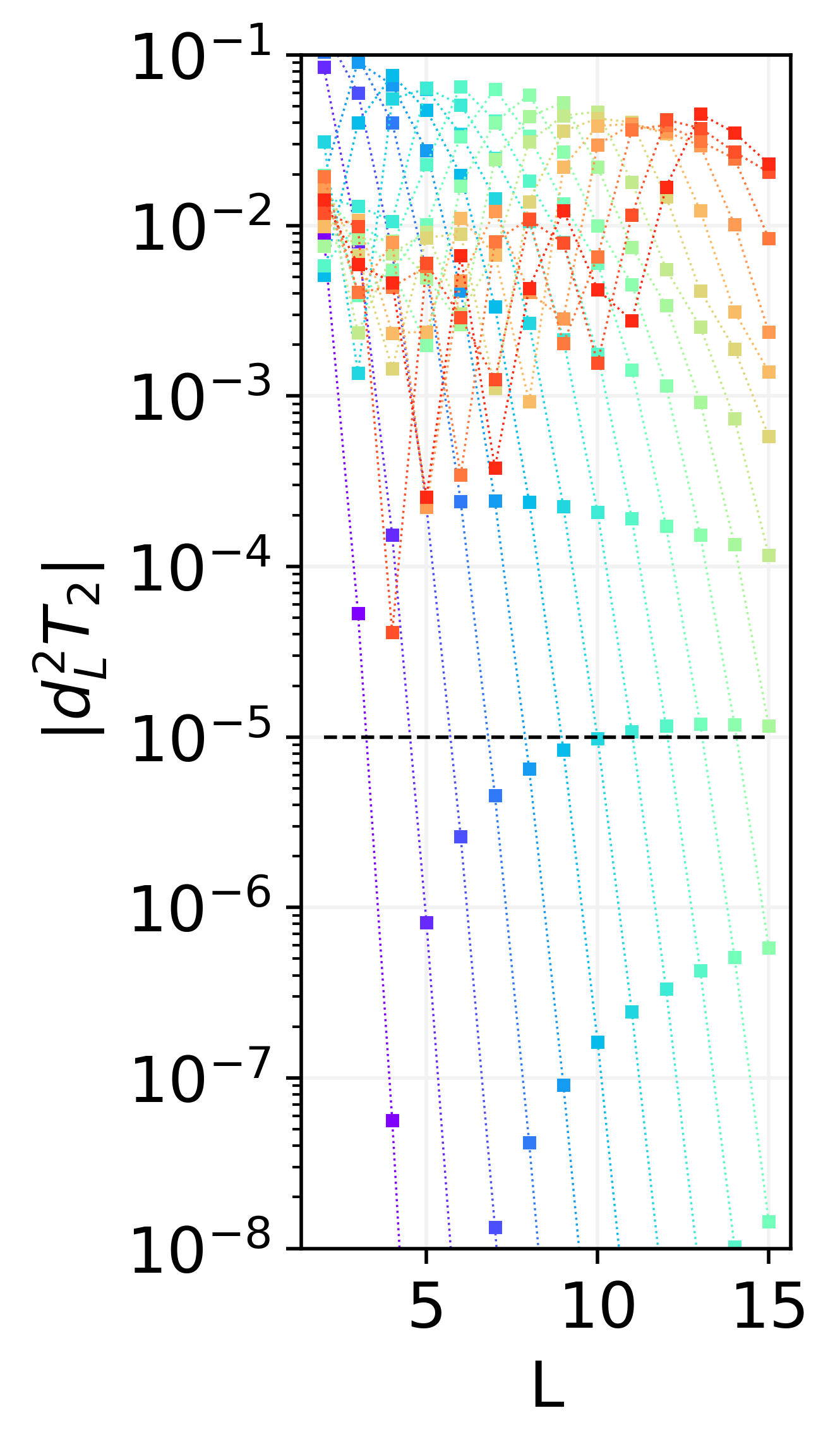
(c)

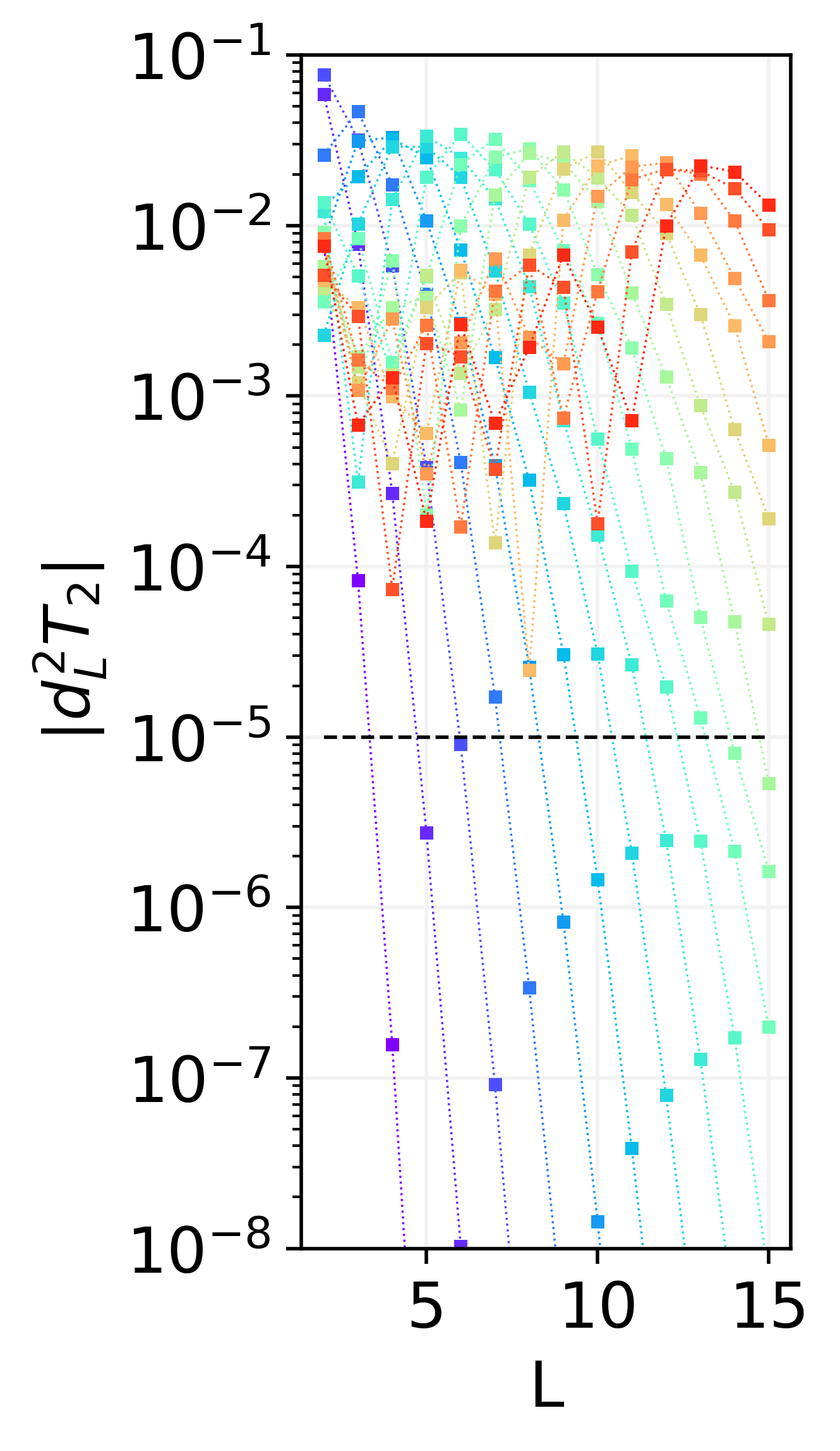
(d)

Figure 5: Second space derivative of $T_{2}(\rho_{L})$ as a function of the subsystem size $L$ after a quench from $\lambda=10^{4}$ to different values of $\lambda^{\prime}$. The subsystem size goes from $2$ to $15$. Different lines represent different times in the range from $0$ (purple line below), to $4$ (red line above). The horizontal black line represents the error tolerance such that functions above the line are definitively exponential. In Panel (a) $\lambda^{\prime}=0.5$; in Panel (b) $\lambda^{\prime}=1.0$ (critical quench); in Panel (c) $\lambda^{\prime}=1.5$; in Panel (d) $\lambda^{\prime}=2.0$.

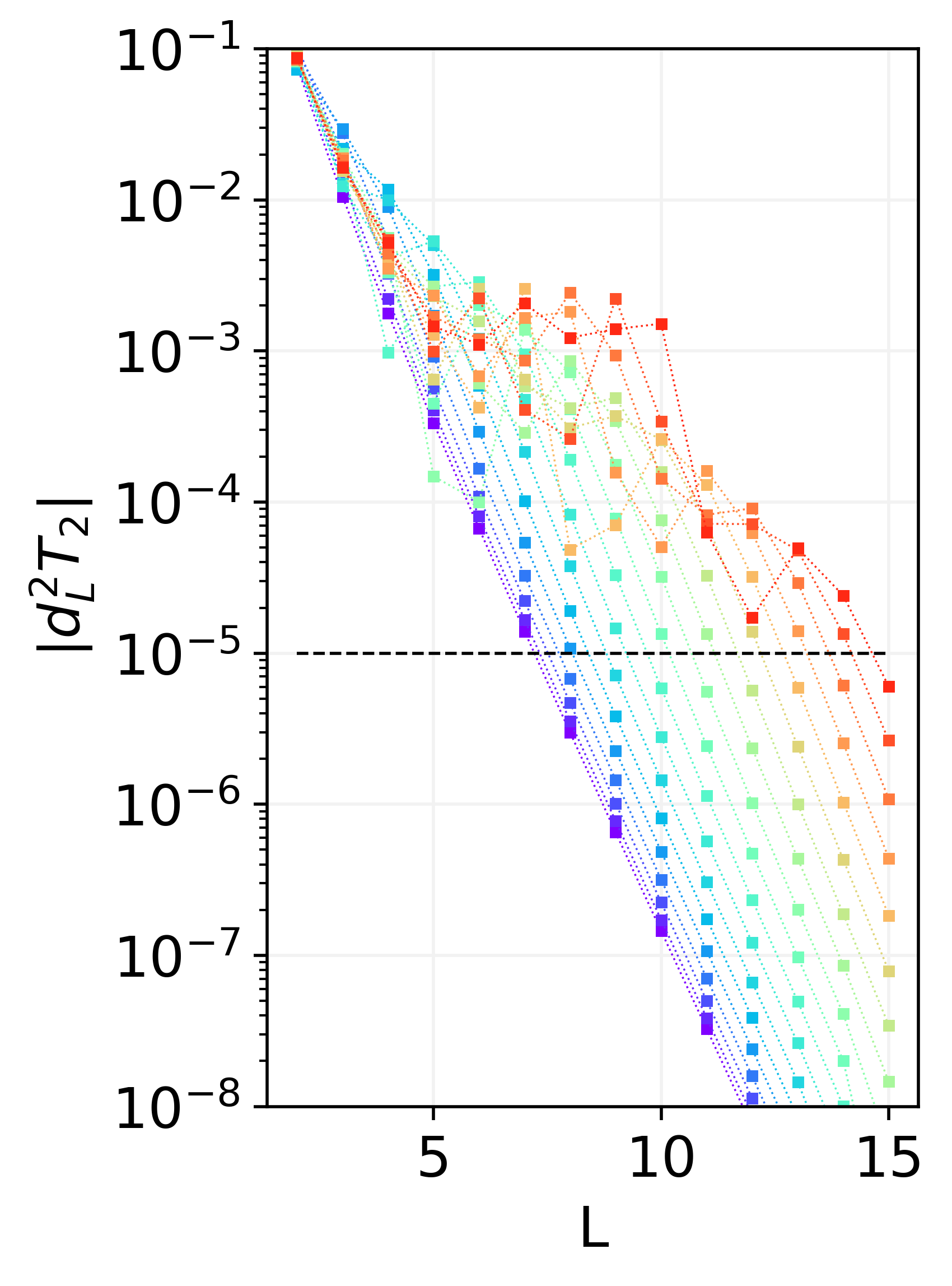
(a)

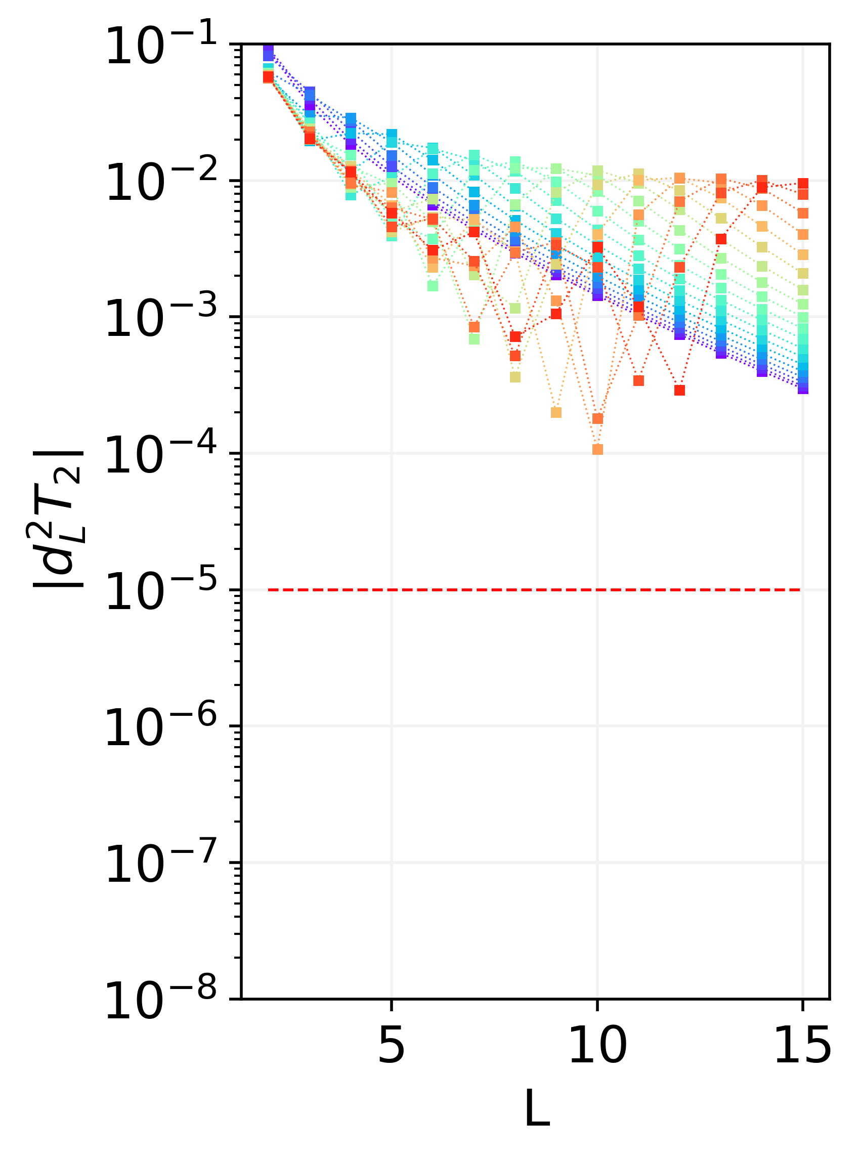
(b)

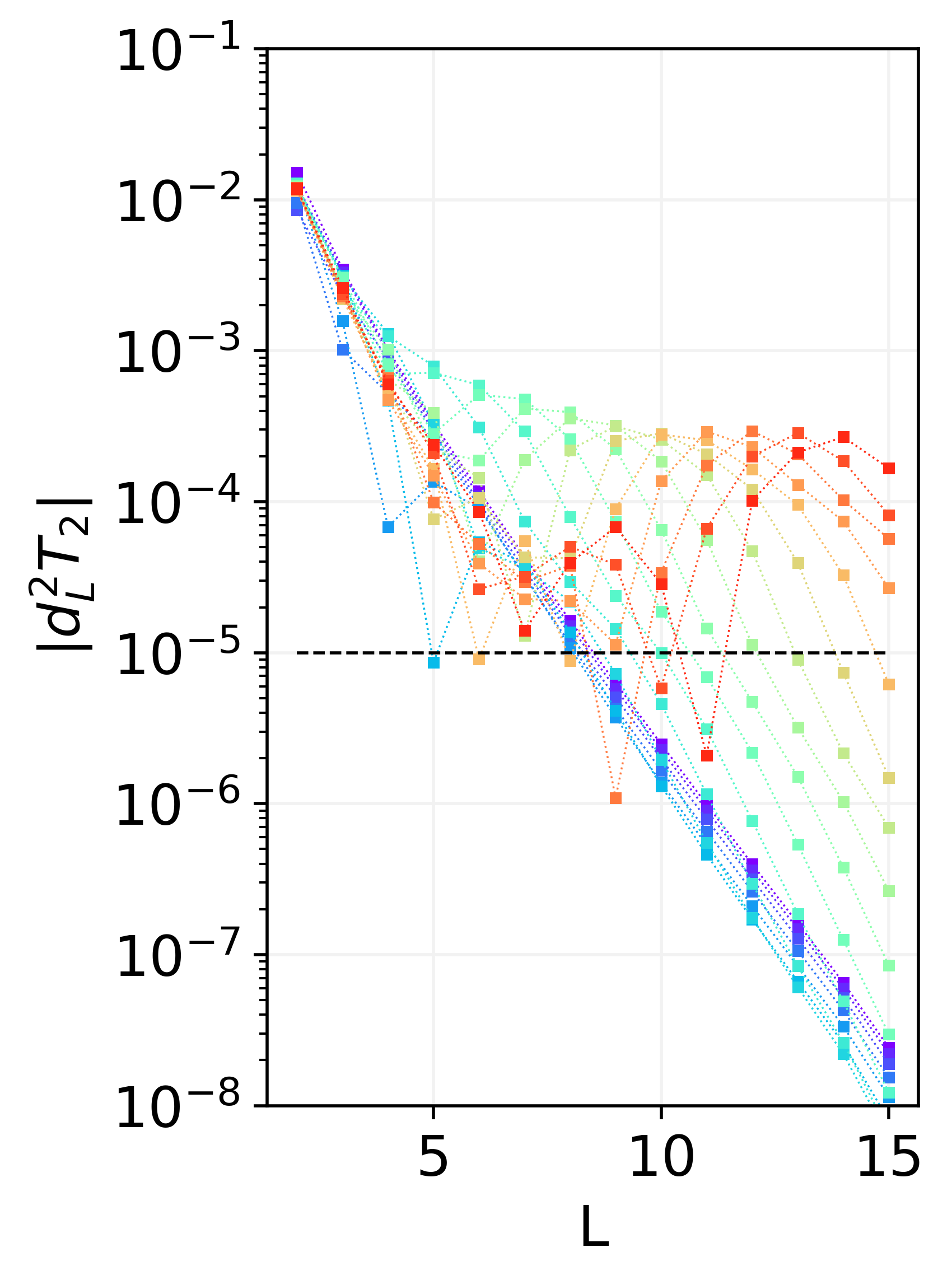
(c)

Figure 6: Second space derivative of $T_{2}(\rho_{L})$ as a function of the subsystem size $L$ after a quench from $\lambda$ to different values of $\lambda^{\prime}=\lambda+0.1$. The subsystem size goes from $2$ to $15$. Different lines represent different times in the range from $0$ (purple line below), to $4$ (red line above). The horizontal black line represents the error tolerance such that functions above the line are definitively exponential. In Panel (a) $\lambda=0.5$; in Panel (b) $\lambda=0.9$ (critical quench); in Panel (c) $\lambda=1.5$.

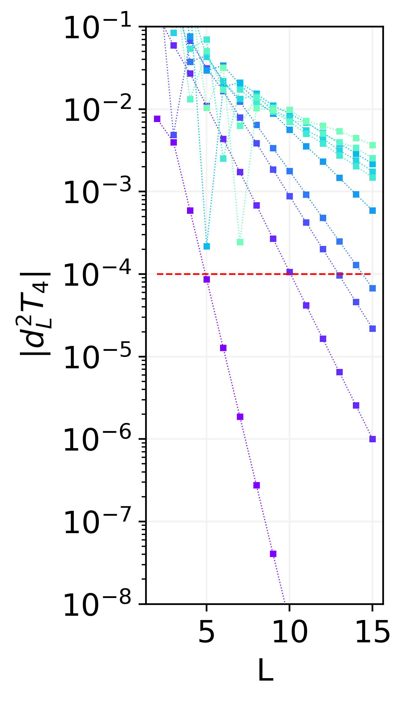
(a)

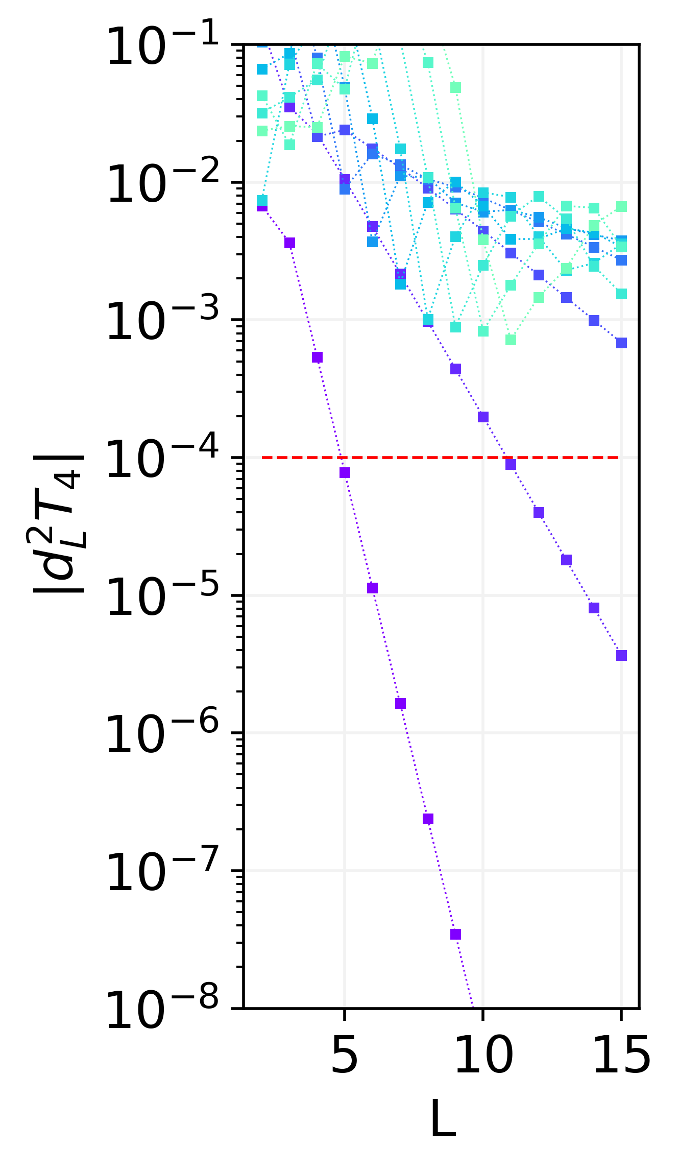
(b)

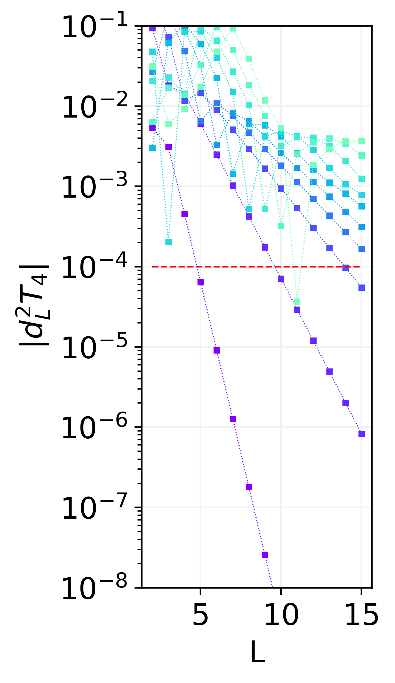
(c)

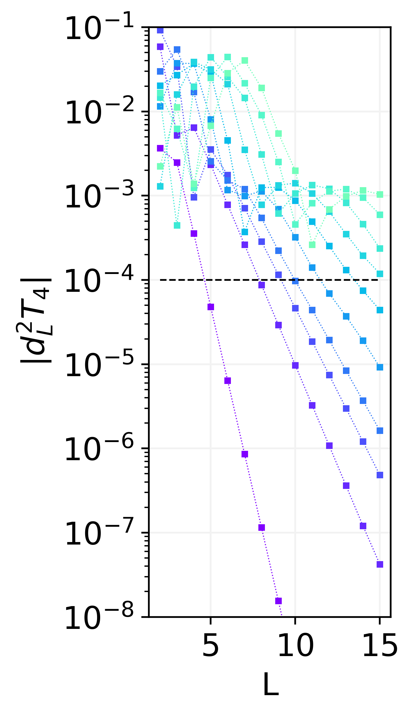
(d)

Figure 7: Second space derivative of $T_{4}(\rho_{L})$ as a function of the subsystem size $L$ after a quench from $\lambda=10^{4}$ to different values of $\lambda^{\prime}$. The subsystem size goes from $2$ to $15$. Different lines represent different times in the range from $0$ (purple line below), to $4$ (red line above). The horizontal black line represents the error tolerance such that functions above the line are definitively exponential. In Panel (a) $\lambda^{\prime}=0.5$; in Panel (b) $\lambda^{\prime}=1.0$ (critical quench); in Panel (c) $\lambda^{\prime}=1.5$; in Panel (d) $\lambda^{\prime}=2.0$.

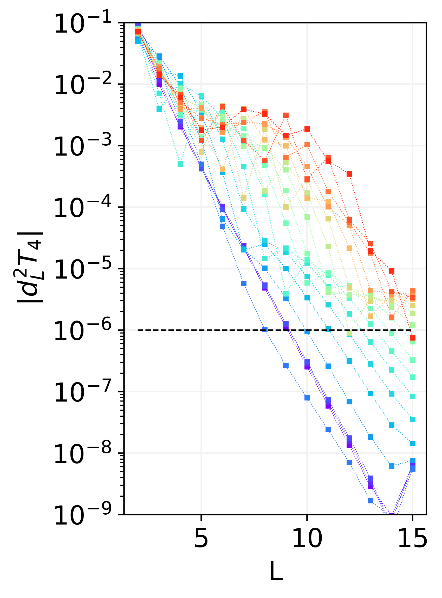
(a)

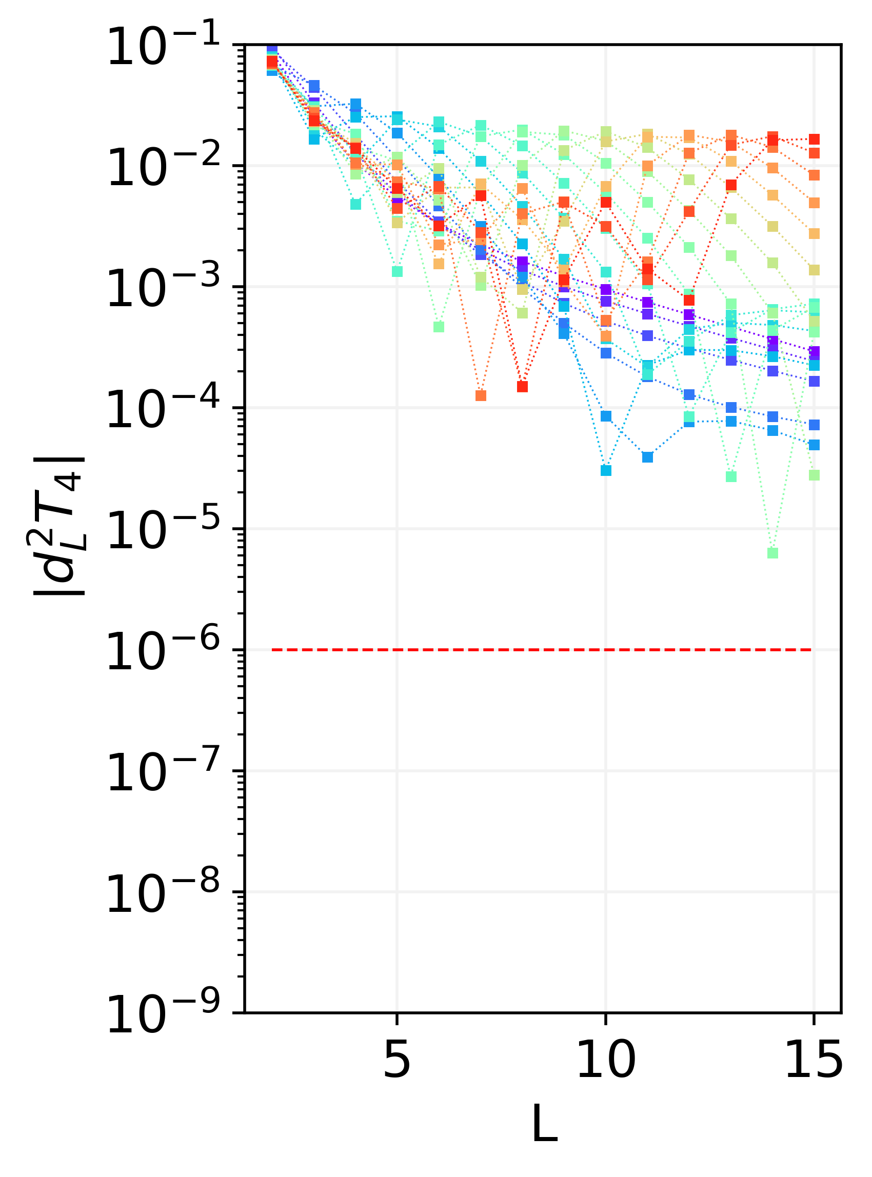
(b)

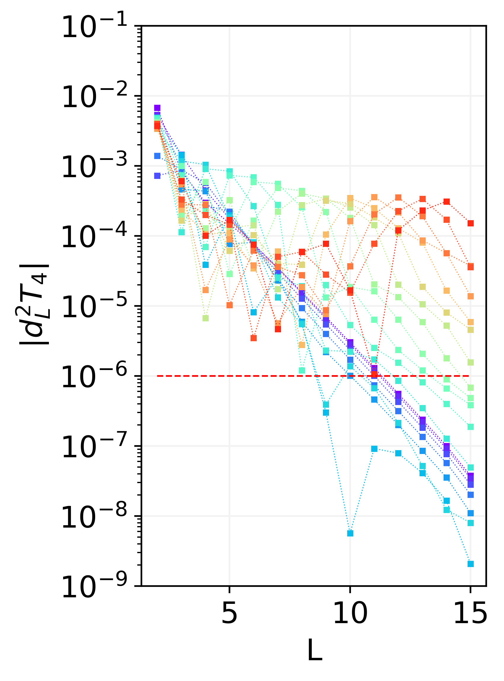
(c)

Figure 8: Second space derivative of $T_{4}(\rho_{L})$ as a function of the subsystem size $L$ after a quench from $\lambda$ to different values of $\lambda^{\prime}=\lambda+0.1$. The subsystem size goes from $2$ to $15$. Different lines represent different times in the range from $0$ (purple line below), to $4$ (red line above). The horizontal black line represents the error tolerance such that functions above the line are definitively exponential. In Panel (a) $\lambda=0.5$; in Panel (b) $\lambda=0.9$ (critical quench); in Panel (c) $\lambda=1.5$.

Appendix C Lieb-Robinson speed

In this Appendix, we analyze the revivals in the Ising model after a quantum quench to reconstruct the associated Lieb-Robinson speed.

In Figure 9 we plot the LE evolution as a function of the rescaled time $t/N$, after the large quench, in Panels (a) and (b), and a large quench, in Panel (c). The revival time is $T_{\text{rev}}\approx N/4$ for $\lambda^{\prime}>1$, and $T_{\text{rev}}\approx N/(\lambda^{\prime}4)$ for $\lambda^{\prime}<1$. Therefore, the associated velocity is $v_{\text{LR}}=2$ for $\lambda^{\prime}>1$, and $v_{\text{LR}}=2\lambda^{\prime}$ for $\lambda^{\prime}<1$. As expected from the fact that the Lieb-Robinson velocity only depends on the quench Hamiltonian, the same behavior is encountered both in the small quench and in the large quench.

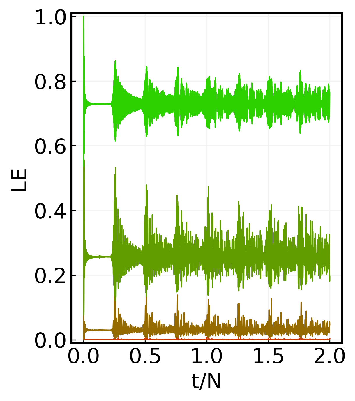
(a)

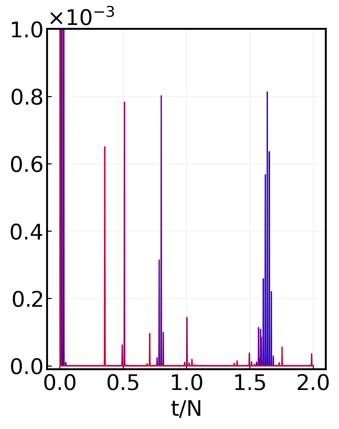
(b)

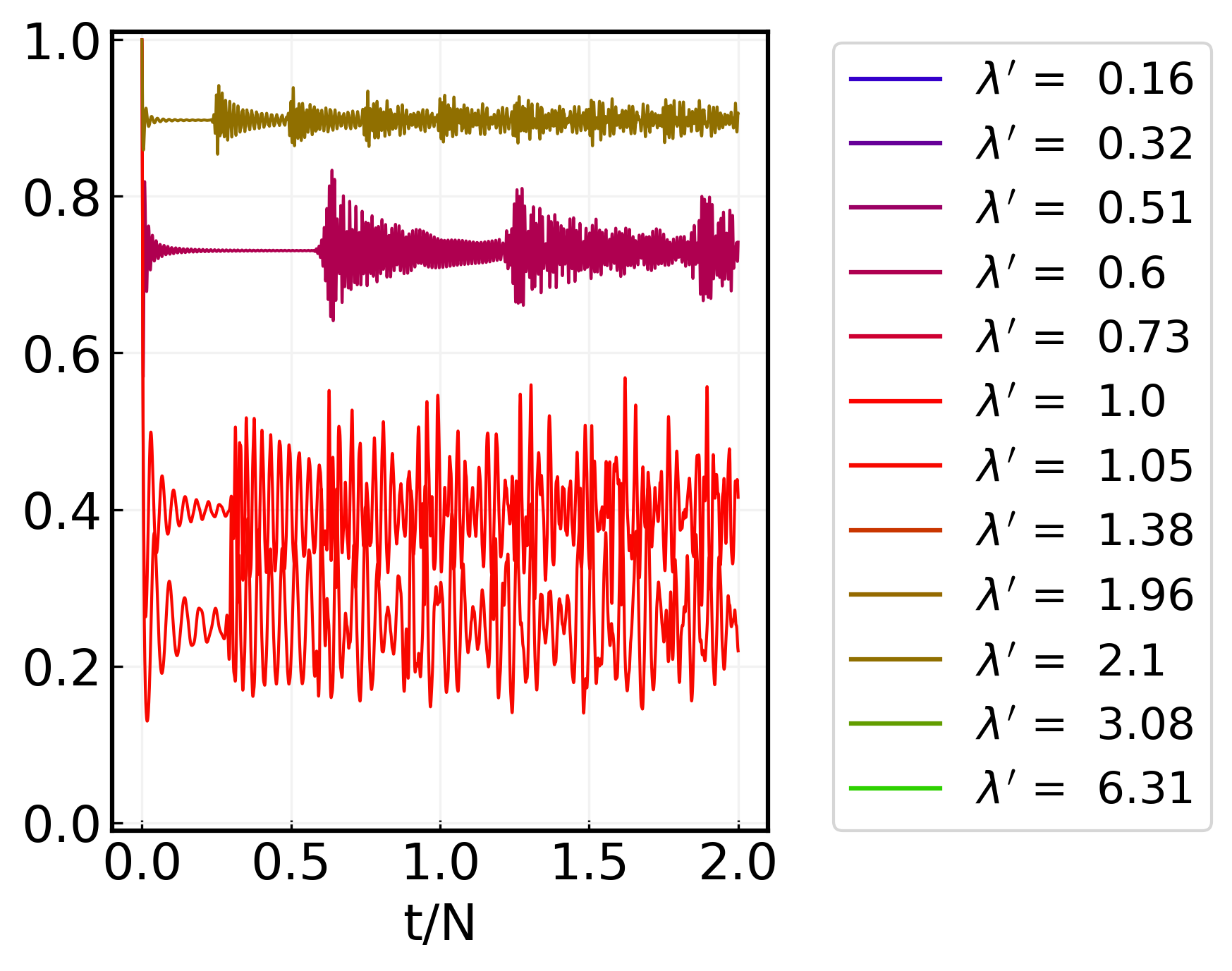
(c)

Figure 9: Evolution of the LE with respect to the rescaled time $t/N$, where $t$ runs from $0$ to $2N$. In Panels (a) and (b) for the large quench protocol where the initial state is $\ket{\psi}\approx\ket{\uparrow\dots\uparrow}$, for a system of $N=100$ spins. In Panel (c) for the small quench protocol where $\lambda^{\prime}=\lambda+0.1$, for a system of $N=200$ spins.

References

- Deutsch and Jozsa (1992) D. Deutsch and R. Jozsa, Proceedings of the Royal Society of London. Series A: Mathematical and Physical Sciences 439, 553 (1992).
- Shor (1994) P. Shor, in Proceedings 35th Annual Symposium on Foundations of Computer Science (1994) pp. 124–134.
- Lloyd (1996) S. Lloyd, Science 273, 1073 (1996).
- Grover (1996) L. K. Grover (Association for Computing Machinery, 1996) pp. 212–219–212–219.
- Kitaev (1997) A. Y. Kitaev, Russian Mathematical Surveys 52, 1191 (1997).
- Abrams and Lloyd (1999) D. S. Abrams and S. Lloyd, Physical Review Letters 83, 5162 (1999).
- Harrow et al. (2009) A. W. Harrow, A. Hassidim, and S. Lloyd, Physical Review Letters 103, 150502 (2009).
- Aspect et al. (1981) A. Aspect, P. Grangier, and G. Roger, Physical Review Letters 47, 460 (1981).
- Aspect et al. (1982a) A. Aspect, P. Grangier, and G. Roger, Physical Review Letters 49, 91 (1982a).
- Aspect et al. (1982b) A. Aspect, J. Dalibard, and G. Roger, Physical Review Letters 49, 1804 (1982b).
- Bell (1964) J. S. Bell, Physics Physique Fizika 1, 195 (1964).
- Fine (1982) A. Fine, Physical Review Letters 48, 291 (1982).
- Terhal (2000) B. M. Terhal, Physics Letters A 271, 319 (2000).
- Werner and Wolf (2001) R. F. Werner and M. M. Wolf, “Bell inequalities and entanglement,” (2001).
- Latorre et al. (2004) J. I. Latorre, E. Rico, and G. Vidal, “Ground state entanglement in quantum spin chains,” (2004), arXiv:quant-ph/0304098.
- Orús (2014) R. Orús, Annals of Physics 349, 117 (2014).
- Gottesman (1998) D. Gottesman, “The Heisenberg Representation of Quantum Computers,” (1998), arXiv:quant-ph/9807006.
- Bravyi and Kitaev (2005) S. Bravyi and A. Kitaev, Physical Review A 71, 022316 (2005).
- Campbell and Browne (2010) E. T. Campbell and D. E. Browne, Physical Review Letters 104, 030503 (2010).
- Campbell and Howard (2017) E. T. Campbell and M. Howard, Physical Review A 95, 022316 (2017).
- Howard and Campbell (2017) M. Howard and E. Campbell, Physical Review Letters 118, 090501 (2017).
- Seddon and Campbell (2019) J. R. Seddon and E. T. Campbell, Proceedings of the Royal Society A: Mathematical, Physical and Engineering Sciences 475, 20190251 (2019).
- Leone et al. (2022a) L. Leone, S. F. E. Oliviero, and A. Hamma, Physical Review Letters 128, 050402 (2022a).
- Leone et al. (2023a) L. Leone, S. F. E. Oliviero, and A. Hamma, Physical Review A 107, 022429 (2023a), publisher: American Physical Society.
- Chamon et al. (2014) C. Chamon, A. Hamma, and E. R. Mucciolo, Physical Review Letters 112, 240501 (2014).
- Yang et al. (2017) Z.-C. Yang, A. Hamma, S. M. Giampaolo, E. R. Mucciolo, and C. Chamon, Physical Review B 96, 020408 (2017).
- Zhou et al. (2020) S. Zhou, Z.-C. Yang, A. Hamma, and C. Chamon, SciPost Physics 9, 87 (2020).
- Liu and Winter (2022) Z.-W. Liu and A. Winter, PRX Quantum 3, 020333 (2022).
- White et al. (2021) C. D. White, C. Cao, and B. Swingle, Physical Review B 103, 075145 (2021).
- Sewell and White (2022) T. J. Sewell and C. D. White, (2022), 10.48550/ARXIV.2201.12367, publisher: arXiv.
- Koukoulekidis and Jennings (2022) N. Koukoulekidis and D. Jennings, npj Quantum Information 8, 1 (2022).
- Hinsche et al. (2022) M. Hinsche, M. Ioannou, A. Nietner, J. Haferkamp, Y. Quek, D. Hangleiter, J.-P. Seifert, J. Eisert, and R. Sweke, “A single $T$-gate makes distribution learning hard,” (2022), arXiv:2207.03140 [quant-ph, stat].
- Leone et al. (2023b) L. Leone, S. F. E. Oliviero, G. Esposito, and A. Hamma, “Phase transition in Stabilizer Entropy and efficient purity estimation,” (2023b), arXiv:2302.07895 [quant-ph].
- Niroula et al. (2023) P. Niroula, C. D. White, Q. Wang, S. Johri, D. Zhu, C. Monroe, C. Noel, and M. J. Gullans, “Phase transition in magic with random quantum circuits,” (2023), arXiv:2304.10481 [quant-ph].
- Oliviero et al. (2022a) S. F. E. Oliviero, L. Leone, A. Hamma, and S. Lloyd, npj Quantum Information 8, 1 (2022a), number: 1 Publisher: Nature Publishing Group.
- Haug and Kim (2023) T. Haug and M. Kim, PRX Quantum 4, 010301 (2023), publisher: American Physical Society.
- Oliviero et al. (2022b) S. F. E. Oliviero, L. Leone, and A. Hamma, Physical Review A 106, 042426 (2022b), publisher: American Physical Society.
- Haug and Piroli (2023a) T. Haug and L. Piroli, Physical Review B 107, 035148 (2023a), publisher: American Physical Society.
- Lami and Collura (2023) G. Lami and M. Collura, “Quantum Magic via Perfect Pauli Sampling of Matrix Product States,” (2023), arXiv:2303.05536 [quant-ph].
- Haug and Piroli (2023b) T. Haug and L. Piroli, “Stabilizer entropies and nonstabilizerness monotones,” (2023b), arXiv:2303.10152 [cond-mat, physics:quant-ph].
- Tirrito et al. (2023) E. Tirrito, P. S. Tarabunga, G. Lami, T. Chanda, L. Leone, S. F. E. Oliviero, M. Dalmonte, M. Collura, and A. Hamma, “Quantifying non-stabilizerness through entanglement spectrum flatness,” (2023), arXiv:2304.01175 [quant-ph].
- Odavić et al. (2022) J. Odavić, T. Haug, G. Torre, A. Hamma, F. Franchini, and S. M. Giampaolo, “Complexity of frustration: a new source of non-local non-stabilizerness,” (2022), arXiv:2209.10541 [cond-mat, physics:quant-ph].
- Chen et al. (2022) L. Chen, R. J. Garcia, K. Bu, and A. Jaffe, “Magic of Random Matrix Product States,” (2022), arXiv:2211.10350 [cond-mat, physics:hep-th, physics:quant-ph].
- Lieb and Robinson (1972) E. H. Lieb and D. W. Robinson, Communications in Mathematical Physics 28, 251 (1972).
- Lieb et al. (1961) E. Lieb, T. Schultz, and D. Mattis, Annals of Physics 16, 407 (1961).
- Pfeuty (1970) P. Pfeuty, Annals of Physics 57, 79 (1970).
- Barouch and McCoy (1971) E. Barouch and B. M. McCoy, Physical Review A 3, 786 (1971).
- Mbeng et al. (2020) G. B. Mbeng, A. Russomanno, and G. E. Santoro, “The quantum ising chain for beginners,” (2020).
- Rigol et al. (2008) M. Rigol, V. Dunjko, and M. Olshanii, Nature 452, 854 (2008).
- Eisert et al. (2015) J. Eisert, M. Friesdorf, and C. Gogolin, Nature Physics 11, 124 (2015).
- Tasaki (1998) H. Tasaki, Physical Review Letters 80, 1373 (1998).
- Reimann (2008) P. Reimann, Physical Review Letters 101, 190403 (2008).
- Linden et al. (2009) N. Linden, S. Popescu, A. J. Short, and A. Winter, Physical Review E 79, 061103 (2009).
- Leone et al. (2021a) L. Leone, S. F. E. Oliviero, Y. Zhou, and A. Hamma, Quantum 5, 453 (2021a).
- Oliviero et al. (2021a) S. F. E. Oliviero, L. Leone, and A. Hamma, Physics Letters A 418, 127721 (2021a).
- Oliviero et al. (2022c) S. F. E. Oliviero, L. Leone, S. Lloyd, and A. Hamma, “Black Hole complexity, unscrambling, and stabilizer thermal machines,” (2022c), arXiv:2212.11337 [gr-qc, physics:hep-th, physics:quant-ph].
- Leone et al. (2022b) L. Leone, S. F. E. Oliviero, S. Lloyd, and A. Hamma, “Learning efficient decoders for quasi-chaotic quantum scramblers,” (2022b), arXiv:2212.11338 [quant-ph].
- Leone et al. (2022c) L. Leone, S. F. E. Oliviero, S. Piemontese, S. True, and A. Hamma, Physical Review A 106, 062434 (2022c), publisher: American Physical Society.
- Campbell et al. (2017) E. T. Campbell, B. M. Terhal, and C. Vuillot, Nature 549, 172 (2017).
- Hastings and Koma (2006) M. B. Hastings and T. Koma, Communications in Mathematical Physics 265, 781 (2006).
- Nachtergaele et al. (2006) B. Nachtergaele, Y. Ogata, and R. Sims, Journal of Statistical Physics 124, 1 (2006), arXiv:math-ph/0603064.
- Eisert (2013) J. Eisert, “Entanglement and tensor network states,” (2013), arXiv:1308.3318 [quant-ph] .
- Alhambra and Cirac (2021) A. M. Alhambra and J. I. Cirac, PRX Quantum 2, 040331 (2021).
- Häppölä et al. (2012) J. Häppölä, G. B. Halász, and A. Hamma, Physical Review A 85, 032114 (2012).
- Dowling et al. (2023) N. Dowling, P. Kos, and K. Modi, “Scrambling is Necessary but Not Sufficient for Chaos,” (2023), arXiv:2304.07319 [cond-mat, physics:hep-th, physics:nlin, physics:quant-ph].
- Leone et al. (2021b) L. Leone, S. F. E. Oliviero, and A. Hamma, Entropy 23 (2021b), 10.3390/e23081073.
- Oliviero et al. (2021b) S. F. E. Oliviero, L. Leone, F. Caravelli, and A. Hamma, SciPost Physics 10, 76 (2021b).
- Dowling and Modi (2023) N. Dowling and K. Modi, “Quantum Chaos = Volume-Law Spatiotemporal Entanglement,” (2023), arXiv:2210.14926 [cond-mat, physics:quant-ph].
- Omanakuttan et al. (2023) S. Omanakuttan, K. Chinni, P. D. Blocher, and P. M. Poggi, Physical Review A 107, 032418 (2023), publisher: American Physical Society.
- Goto et al. (2022) K. Goto, T. Nosaka, and M. Nozaki, Physical Review D 106, 126009 (2022), publisher: American Physical Society.
- True and Hamma (2022) S. True and A. Hamma, Quantum 6, 818 (2022), publisher: Verein zur Förderung des Open Access Publizierens in den Quantenwissenschaften.
- Kim et al. (2023) J. Kim, Y. Oz, and D. Rosa, Journal of Statistical Mechanics: Theory and Experiment 2023, 023104 (2023), publisher: IOP Publishing.