Preserving Superconvergence of Spectral Elements for Curved Domains via $h$ and $p$-Geometric Refinement

Abstract

Spectral element methods (SEM), which are extensions of finite element methods (FEM), are important emerging techniques for solving partial differential equations in physics and engineering. SEM can potentially deliver better accuracy due to the potential superconvergence for well-shaped tensor-product elements. However, for complex geometries, the accuracy of SEM often degrades due to a combination of geometric inaccuracies near curved boundaries and the loss of superconvergence with simplicial or non-tensor-product elements. We propose to overcome the first issue by using $h$- and $p$-geometric refinement, to refine the mesh near high-curvature regions and increase the degree of geometric basis functions, respectively. We show that when using mixed-meshes with tensor-product elements in the interior of the domain, curvature-based geometric refinement near boundaries can improve the accuracy of the interior elements by reducing pollution errors and preserving the superconvergence. To overcome the second issue, we apply a post-processing technique to recover the accuracy near the curved boundaries by using the adaptive extended stencil finite element method (AES-FEM). The combination of curvature-based geometric refinement and accurate post-processing delivers an effective and easier-to-implement alternative to other methods based on exact geometries. We demonstrate our techniques by solving the convection-diffusion equation in 2D and show one to two orders of magnitude of improvement in the solution accuracy, even when the elements are poorly shaped near boundaries.

1 Introduction

Spectral element methods (SEM) are extensions of finite element methods (FEM) that use Gauss-Lobatto or similar nodes instead of equidistant nodes for high-order elements karniadakis2005spectral . Mathematically, SEM with well-shaped tensor-product elements can deliver higher accuracy than equidistant FEM due to potential superconvergence kvrivzek1987superconvergence ; Chen1995 ; Zlamal1977 ; Zlamal1978 , in that the $\ell_{2}$-norm error (i.e., nodal solution error) may converge faster (at $(p+2)$nd order with degree-$p$ elements kvrivzek1987superconvergence ; Chen1995 ; Zlamal1977 ; Zlamal1978 ) than the standard “optimal” rate of the $L_{2}$ norm (at $(p+1)$st order) of FEM. However, some significant challenges remain for domains with curved boundaries, limiting the advantages of SEM for some real-world applications. In particular, non-tensor-product elements are typically used near boundaries, leading to the loss of superconvergence of the overall solution. In addition, for curved domains, isoparametric elements are commonly used, for which the geometry is approximated to the same order as the solution space. There has been significant evidence in isogeometric analysis hughes2005isogeometric ; scott2011isogeometric and NURBS-enhanced FEM (NEFEM) sevilla2008nurbs ; sevilla2011comparison that a more accurate boundary representation can significantly improve the overall accuracy of the solutions. Similar observations have been made in the context of discontinuous Galerkin methods botti2018assessment . However, to the best of our knowledge, there has not been a systematic study on the issue in the context of continuous Galerkin formulations with high-order finite or spectral elements.

In this work, we propose a novel approach to improve the overall accuracy and preserve the superconvergence of SEM over curved domains. Our approach has two distinct components. First, we develop a mesh-generation procedure using rectangular tensor-product elements in the interior of the domain but geometrically refined non-tensor-product elements near curved boundaries. The geometric refinement includes curvature-based edge-length controls and optionally superparametric elements, which we refer to as $h$- and $p$-geometric refinements ($h$-GR and $p$-GR), respectively. We show that the refinements can improve the accuracy of the geometric representations and, in turn, reduce the pollution errors of the tensor-product elements in the interior of the domain. Second, we propose a post-processing phase to improve the accuracy of the near-boundary elements using the adaptive extended stencil finite element method (AES-FEM) conley2016overcoming ; conley2020hybrid , so that the accuracy of non-tensor-product elements can match those of the superconvergent spectral elements. Overall, we show that our approach can deliver one to two orders of improvement in solution accuracy.

The contributions of the work can be summarized as follows. First, to the best of our knowledge, it is the first work to demonstrate the superconvergence of SEM over curved domains with both Dirichlet and Neumann boundary conditions. This result is significant in that theoretical analysis of superconvergence is limited to only Dirichlet boundary conditions over rectangular domains kvrivzek1987superconvergence ; Chen1995 ; Zlamal1977 ; Zlamal1978 . Second, we show that contrary to the conventional wisdom of isoparametric elements strangfem , superparametric elements can play an important role in improving the accuracy of nodal solutions, especially when combined with $h$-GR. Third, we show that the impact of geometric refinements may be orders of magnitude more significant than the element shapes for FEM and SEM. These results suggest that we should focus on geometric accuracy instead of element shapes for high-order elements. Fourth, our overall workflow offers a promising alternative to other discretization methods using exact geometries, such as NEFEM sevilla2008nurbs ; sevilla2011comparison . Our approach is easier to implement because its mesh generation and adaptation procedure is more consistent with standard FEM and SEM. Its post-processing step can be incorporated into other superconvergence post-processing steps with a relatively small computational cost.

The remainder of the paper is organized as follows. In section 2, we present some background information on SEM and related pre- and post-processing techniques. In section 3, we discuss the reasons for the loss of superconvergence of SEM in the presence of curved boundaries and some potential remedies. In section 4, we describe our mesh-generation procedure, focusing on $h$- and $p$-GR and the placement of high-order nodes in 2D, with a brief discussion on the extension to 3D. In section 5, we present numerical results and demonstrate the impact of geometric refinement on the preservation of superconvergence. Section 6 concludes the paper.

2 Background

We first review FEM and SEM, focusing on their superconvergence properties and pre- and post-processing techniques over curved domains.

2.1 Finite and Spectral Element Methods

Mathematically, FEM and SEM are spatial discretization techniques for partial differential equations (PDEs). For simplicity, let us consider linear elliptic PDEs, such as the convention-diffusion equation, which we will solve in section 5. Let $\Omega\subset\mathbb{\mathbb{R}}^{d}$ be a bounded, piecewise smooth domain with boundary $\partial\Omega=\Gamma_{D}\cup\Gamma_{N}$, where $\Gamma_{D}$ and $\Gamma_{N}$ denote the Dirichlet and Neumann boundaries, respectively. Typically, $d=2$ or 3. Let $\mathcal{L}$ be a second-order elliptic linear differential operator. The associated boundary value problem is to find a sufficiently smooth solution $u$ such that

$$\mathcal{L}u=f \quad\text{on }\Omega,$$ (1)

$$u=u_{D} \quad\text{on }\Gamma_{D},$$ (2)

$$\partial_{\boldsymbol{n}}u=g_{N} \quad\text{on }\Gamma_{N},$$ (3)

where $u_{D}$ denotes the Dirichlet boundary conditions and $g_{N}$ denotes the Neumann boundary conditions. The domain $\Omega$ is tessellated into a mesh, composed of a set of elements. FEM and SEM approximate the solution to equations (1)–(3) using the method of weighted residuals finlayson2013method . Let $u_{h}$ denote the approximate solution, and the residual of equation (1) is then $\mathcal{L}u_{h}-f$. Let $\Psi=\left\{\psi_{i}\mid 1\leq i\leq n\right\}$ denote a set of test functions. A weighted residual method requires the residual to be orthogonal to $\Psi$ over $\Omega$, that is,

$$\int_{\Omega}\mathcal{L}u_{h}\psi_{i}\ d\Omega=\int_{\Omega}f\psi_{i}\ d\Omega,\quad\text{for }i=1,\dots,n.$$

Traditionally, FEM uses equidistant nodes within each element and the basis functions for $u_{h}$ are piecewise Lagrange polynomial basis functions based on these nodes. In contrast, SEM uses Gauss-Lobatto nodes over tensor-product elements patera1984spectral ; maday1990optimal ; karniadakis2005spectral , based on the tensor-product Gauss-Lobatto quadrature rules. One of the motivations for using Gauss-Lobatto points is the improved stability of polynomial interpolations for very high-degree polynomials. However, for moderate degrees, the major advantage of SEM is that the nodal solutions naturally superconverge, in the sense that the $\ell_{2}$-norm error is $\mathcal{O}(h^{p+2})$ for degree-$p$ elements chen1981superconvergence , whereas the optimal convergence rate in $L_{2}$ norm is only $\mathcal{O}(h^{p+1})$ strangfem , where $h$ denotes an edge-length measure, assuming the mesh is quasi-uniform.

The superconvergence property of tensor-product SEM has been studied extensively in the literature; we refer readers to brenner2004finite ; zhu1998review and references therein. In a nutshell, the superconvergence is related to the fact that the Gauss-Lobatto polynomials are derivatives of Legendre polynomials chen1981superconvergence . However, this connection with orthogonal polynomials does not generalize to non-tensor-product elements, regardless of whether they are obtained by degenerating tensor-product elements karniadakis2005spectral or using some Gauss-Lobatto-like point distributions (such as Fekete points taylor2000algorithm ). Hence, non-tensor-product “spectral” elements generally do not superconverge. Nevertheless, they are useful for compatibility with tensor-product spectral elements in mixed-element meshes (see e.g., karniadakis2005spectral ; komatitsch2001wave ), which are desirable to handle complex geometries arising from engineering applications. In this work, we use mixed-element meshes as in karniadakis2005spectral ; komatitsch2001wave . Still, we aim to preserve the superconvergence of tensor-product elements and, in addition, improve the accuracy of the non-tensor-product element.

2.2 Resolution of Curved Boundaries in Finite Element Analysis (FEA)

Curved boundaries have long been recognized as a significant source of error in FEA because insufficient geometric accuracy can lead to suboptimal convergence rates (see e.g., cheung2019optimally ; luo2001influence ). Traditionally, isoparametric elements were believed to be sufficient to preserve the $\mathcal{O}(h^{p+1})$ accuracy in $L_{2}$ norm strangfem . Nevertheless, superparametric elements, in which the degree of the geometric basis functions is greater than the degree of the trial space (see e.g., eslami2014finite ), have been shown to improve accuracy in the context of discontinuous Galerkin methods zwanenburg2017necessity ; bassi1997high . In this work, we will show that superparametric elements can also significantly improve accuracy for continuous Galerkin methods in $\ell_{2}$ norm (i.e., nodal solutions), especially for Neumann boundary conditions, thanks to the improved accuracy in normal directions.

In recent years, some alternatives have been developed to improve geometric accuracy. Most notably, isogeometric analysis (IGA) hughes2005isogeometric and NURBS-enhanced finite element method (NEFEM) sevilla2008nurbs ; sevilla2011comparison use exact geometries. IGA is analogous to isoparametric FEM, using the same basis functions for the geometric representation and the solutions. Since geometric models (such as NURBS) typically use $C^{1}$ or $C^{2}$ basis functions, IGA has higher regularity of its solutions, allowing it to resolve smoother functions more effectively in some applications. In contrast, NEFEM is analogous to superparametric FEM in that it uses the exact geometric representation while preserving the Lagrange polynomial basis of the trial and test spaces of FEM. Both IGA and NEFEM pose significant challenges in mesh generation for complex domains.

2.3 Curvature-Based Mesh Generation and Adaptation

Using superparametric elements or exact geometry increases the degree of the geometric representations. In addition, one can also improve geometric accuracy by adapting the edge length based on curvature. Such an approach is relatively popular in computer graphics and visualization; see e.g., the survey paper khan2020surface and references therein. For example, in dassi2014curvature , Dassi et al. introduced an optimization-based surface remeshing method, whether the energy is defined based on curvatures. In mansouri2016segmentation , Mansouri and Ebrahimnezhad used Voronoi tesselation and Lloyd’s relaxation algorithm lloyd1982least to create curvature adaptive site centers. These site centers are used to generate a curvature-based mesh. In the context of FEM, Moxey et al. moxey2015isoparametric generated boundary layer meshes based on curvatures. In this work, we use the radii of curvatures to guide the refinement of edge lengths. We also use it in conjunction with superparametric elements to improve geometric accuracy, to reduce the pollution errors of the spectral elements in the interior of the domain.

2.4 Superconvergent Post-Processing Techniques

An important technique in this work is to post-process the solutions near boundaries to recover higher accuracy near boundaries. To this end, we use AES-FEM, a method based on weighted least-squares approximations conley2016overcoming ; conley2020hybrid . We defer more detailed discussions on AES-FEM to section 3.2. In FEM, post-processing is often used to improve the accuracy of the solutions or gradients. For example, Bramble and Schatz bramble1977higher developed a post-processing method to achieve superconvergence of the solution using an averaging method, but the technique requires the mesh to be locally translation invariant. In Babuska1984 , Babuška and Miller constructed generating functions to compute weighted averages of solutions over the entire finite element domain, but the method did not produce superconvergent results. The post-processing of gradients has enjoyed better success. One such technique is the superconvergent patch recovery (SPR) method, which constructs a local polynomial fitting on an element patch and then evaluates the fittings at Gaussian quadrature points to achieve superconvergent first derivatives Zienkiewicz1992b . Other examples include the polynomial preserving recovery (PPR) method Naga2004 and recovery by equilibrium in patches (REP) Boroomand1997 ; Boroomand1997a , which also construct local polynomial fittings. One similarity of these post-processing techniques with AES-FEM is using some form of least-squares fittings. However, unlike those techniques, AES-FEM uses weighted least-squares to compute differential operators and then uses them to solve the PDEs to achieve superconvergent solutions.

3 Spectral Elements over Curved Domains

As discussed in section 2.1, spectral elements can enjoy superconvergence over rectangular domains, but curved domains pose several challenges. We discuss these challenges and the potential remedies in this section.

3.1 Loss and Preservation of Superconvergence

The theoretical analysis of SEM’s superconvergence property is generally limited to rectangular domains with homogeneous (Dirichlet) boundary conditions Chen1995 ; chen1999superconvergence ; Chen2005 . The extension of such analysis to curved domains with general boundary conditions has fundamental challenges, and this work aims to address these challenges. First, the most systematic analyses, such as element orthogonality analysis (EOA) and orthogonality correction technique (OCT) chen1981superconvergence ; Chen1995 ; Chen2005 ; chen2013highest , rely on the properties of orthogonal polynomials. However, the orthogonality is lost if tensor-product elements are used near curved boundaries. Mathematically, this loss is because the Lagrange basis functions in SEM (as in FEM) within each element, say $\phi_{i}(\boldsymbol{x})$, are defined as

$$\phi_{i}(\boldsymbol{x})=\phi_{i}(\boldsymbol{\xi}(\boldsymbol{x})),$$

where $\boldsymbol{\xi}(\boldsymbol{x})$ is the inverse of the mapping

$$\boldsymbol{x}(\boldsymbol{\xi})=\sum_{k=1}^{n_{e}}\boldsymbol{x}_{k}\varphi_{k}(\boldsymbol{\xi}).$$

In the above, $\boldsymbol{\xi}$ denotes the local (or natural) coordinates within an element $\tau$, and $\varphi_{k}(\boldsymbol{\xi})$ denotes the geometric basis function corresponding to the $k$th node of $\tau$. Although the $\phi_{i}(\boldsymbol{\xi})$ and $\varphi_{k}(\boldsymbol{\xi})$ are polynomials, the $\phi_{i}(\boldsymbol{x})$ are no longer polynomials if $\boldsymbol{x}(\boldsymbol{\xi})$ is nonlinear, and as a result, orthogonality is also lost. Hence, we cannot expect superconvergence of the spectral elements near boundaries even if tensor-product spectral elements are used. It is worth noting that this loss of orthogonality also applies to the interior of the domain if the tensor-product elements are skewed (i.e., no longer rectangular). Therefore, we use rectangular spectral elements in the interior of the domain as much as possible. Near boundaries, it suffices to use non-tensor-product elements for more flexibility in mesh generation. These elements cannot superconverge, and we address their accuracy issues in section 3.2.

Second, even if rectangular spectral elements are used in the interior of the domain, the nodal solutions of those elements may still lose superconvergence if the near-boundary elements are too inaccurate because the stiffness matrix couples the nodal solutions of all the elements. We refer to these potential errors in the spectral elements due to inaccurate near-boundary elements as pollution errors. These pollution errors are especially problematic when Neumann boundary conditions are applied to curved boundaries with isoparametric elements since the normal directions are, in general, a factor of $1/h$ less accurate than the nodal positions. For elliptic PDEs, these pollution errors decay with respect to the distance to the boundary. Nevertheless, it is important to reduce the errors of near-boundary elements as much as possible. This analysis motivates the $h$- and $p$-GR that we will describe in section 4. We will verify this analysis numerically in section 5.

3.2 Recovery of Accuracy Near Boundaries

As noted above, the superconvergence is lost for non-tensor-product elements near boundaries. In other words, the nodal solutions near boundaries will be limited to only $\mathcal{O}(h^{p+1})$. Note that this limitation cannot be overcome using $h$-adaptivity within the FEM framework since the non-tensor-product elements directly adjacent to tensor-product elements cannot decrease the edge length. Neither can it be overcome using $p$-adaptivity with non-conformal meshes since the continuity constraints of non-conformal meshes would cause the tensor-product elements to lose superconvergence.

To overcome this fundamental challenge, we utilize the high-order adaptive extended stencil finite element method (AES-FEM) as described in conley2020hybrid . AES-FEM is a generalized weighted residual method, of which the trial functions are generalized Lagrange polynomial (GLP) basis functions constructed using local least squares fittings, but the test functions are $C^{0}$ continuous Lagrange basis functions as in FEM. As shown in conley2020hybrid , on a sufficiently fine quasiuniform mesh with consistent and stable GLP basis functions, the solution of a well-posed even-degree-$p$ AES-FEM for a coercive elliptic PDE with Dirichlet boundary conditions converges at $\mathcal{O}(h^{p})$ in $\ell^{\infty}$ norm, if $p=2$ or if $p>2$ and the local support is nearly symmetric. We refer readers to conley2020hybrid for more details. In this work, we apply AES-FEM as a post-processing step for near-boundary elements by splitting the near-boundary elements into linear elements, as we describe in section 4.4.

4 Curvature-Based $h$- and $hp$-Geometric Refinement

We now describe the generation of mixed-element meshes, which is the core of this work. We describe the mesh-generation process in two dimensions and then outline how the process can be extended to three dimensions.

4.1 Initial Mesh Setup

To recover the high accuracy of SEM, we generate mixed-element meshes using tensor-product elements in the interior of the geometric domain as much as possible with triangular elements near curved boundaries. To this end, we first generate a uniform quadrilateral mesh to cover the bounding box of the domain. Next, we tag the nodes outside the computational domain or within some fixed distance of a curved boundary, where the distance is based on the average edge length of the initial mesh. We then remove these nodes along with any quadrilateral containing them. This process leaves a collection of connected edges that are inside the geometric domain. We then mesh the gap between these edges and the curved boundary using an off-the-shelf mesh generator. In this work, we used MATLAB’s built-in PDE Toolbox PDEToolbox , of which the mesh generator built on top of CGAL cgal:eb-23a . This mesh generator allows nodes to be placed exactly on the curved boundary. We apply $h$-GR adaptivity outlined in section 4.2 during this phase. The nodes from the original quadrilateral mesh and the new triangle mesh are matched so that those duplicate nodes can be removed. The first couple of steps of the mesh generation are shown in Figure 1. Next, the element connectivity table is built using the half-facet array algorithm outlined in AHF . The resulting linear mesh might still have triangles with more than one facet on the curved boundary. These elements could be problematic as placing high-order edge nodes can cause the two facets to “flatten out” and create a negative Jacobian determinant at the corner node where the two curved edges intersect. We use a simple edge flip to prevent this case and ensure that all triangles have only one boundary facet. This process gives a good-quality linear finite element mesh. However, if stronger mesh quality constraints are required, we can also further improve it by using mesh-smoothing techniques, such as that in jiao2011simple .

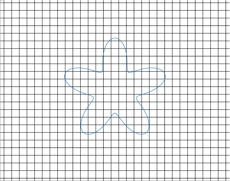
(a) Initial structured mesh and curved boundary $\Gamma$

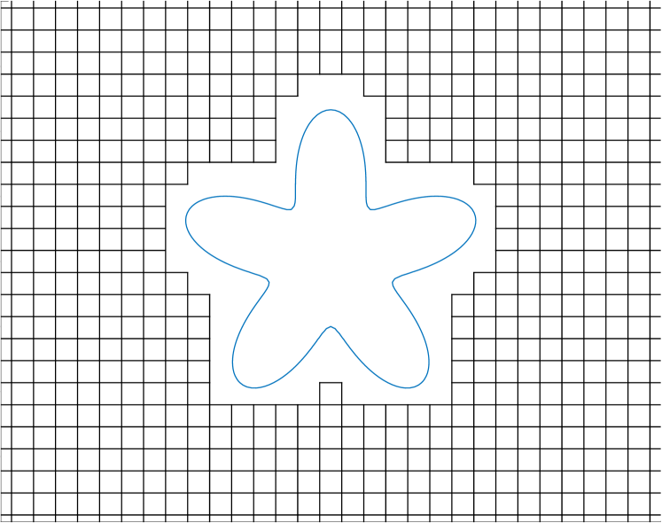
(b) After removing elements outside or on $\Gamma$

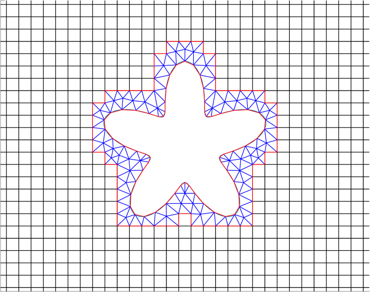
(c) After generating conformal triangles

Figure 1: Steps to generate initial linear mesh.

4.2 Applying $h$-GR

To apply $h$-GR, we seek to generate a local edge length $h$ at each node on the boundary, which is linearly related to the curvature of the boundary. This step is relatively simple and adds negligible computational cost to the mesh generation. We evaluate the curvature for each node on the curved boundary using either the explicit parameterization or some form of geometric reconstruction. Next, we define a target angle $\theta_{max}$ such that no two adjacent nodes have a difference in the normal direction that is greater than $\theta_{max}$. To this end, we make the target edge length the arc length of the circle defined by the radius of curvature and $\theta_{max}$. The edge length at node $i$ is based on the radius of curvature and can be defined as $h_{i}=\theta_{max}R_{i}=\theta_{max}/K_{i}$ where $R_{i}$ is the radius of curvature and $K_{i}$ is the unsigned curvature for node $i$. Since $h_{i}$ defined in this way can be arbitrarily large or small, we limit the minimum and maximum edge lengths using parameters $h_{min}$ and $h_{max}$, respectively. The overall formula for computing the target edge length at node $i$ is defined as

$$h_{i}=\mathrm{min}(\mathrm{max}(\theta_{max}/K_{i},h_{min}),h_{max}).$$

These edge lengths are supplied to the mesh generator as target edge lengths for generating the mesh near the boundary. A mesh with and without $h$-GR adaptivity is displayed in Figure 2.

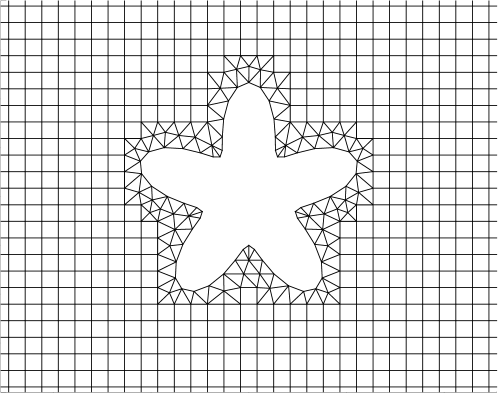
(a) Mesh without $h$-GR

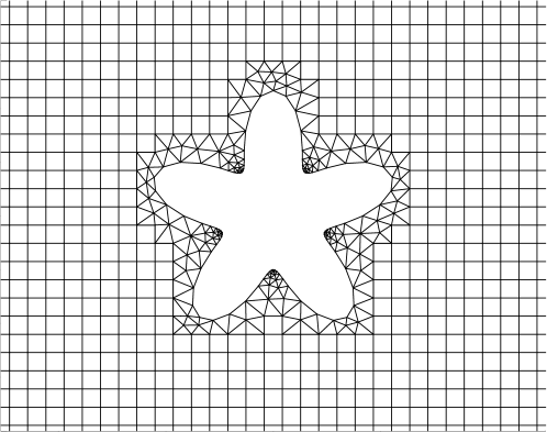
(b) Mesh with $h$-GR

Figure 2: Example meshes around a flower hole with and without curvature-based refinement.

4.3 Placing High-Order Nodes

After obtaining the initial linear mesh, we insert mid-edge and mid-face nodes to generate high-order spectral elements. For the rectangular elements in the interior of the domain, we insert Gauss-Lobatto points to generate tensor-product spectral elements. For the near-boundary elements, we also use Gauss-Lobatto nodes for the facets (i.e., edges) shared between tensor-product and non-tensor-product elements to ensure continuity. The placements of mid-face nodes of triangles are more flexible; we place them at quadrature points that maximize the degree of the quadrature rule as Gauss-Lobatto points do for tensor-product elements. If an element has a curved edge, however, the placement of the nodes needs to satisfy the so-called Ciarlet-Raviart condition ciarlet1972combined to preserve the convergence rate. In a nutshell, the Ciarlet-Raviart condition requires the Jacobian determinant of a degree-$p$ element to have bounded derivatives up to $(p+1)$st order li2019compact . To satisfy the condition, we use an iterative process similar to the one presented in li2019compact . In particular, to generate high-order curved elements with degree-$p$ polynomial basis functions, starting from $q=2$, we incrementally generate a degree-$q$ element by first interpolating the nodal positions using a degree-$(q-1$) element and then project the nodes on curved edges onto the exact geometry. We repeat the process until $q=p+2$, then interpolate the nodal positions of the degree-$p$ element from the degree-$(p+2)$ element. In this fashion, we found that the Jacobian determinant is sufficiently smooth to reduce the pollution errors of the spectral elements. Note that this process is needed only for elements directly incident on curved boundaries, so its computational cost is less complex than the rest of the mesh-generation process.

4.4 Extraction of near boundary elements for AES-FEM

To utilize AES-FEM near the boundary, we need a linear mesh. To this end, we construct a new, smaller, linear mesh from pieces of the high-order mesh. We first decompose the triangular part of the mesh and include all newly generated linear triangles in the AES-FEM mesh. Choosing just the decomposed triangles from the original mesh will not be sufficient to improve accuracy. We must extend into the quadrilateral section of the mesh by a number of layers. A layer is defined as all quadrilaterals with two or more nodes as part of the AES-FEM mesh.

For this reason, we keep a boolean array of all nodes currently in the AES-FEM mesh. Care must be taken as too few elements will result in only minor improvement by AES-FEM, while too many elements will waste computing power (although it will be stable). In practice, two layers typically suffice, and one layer may also suffice for quadratic meshes of simple domains such as the elliptical hole domain. After all the quadrilaterals have been identified, they are decomposed into linear elements and then split into triangles and added to the AES-FEM mesh. Figure 3 shows an example of an extracted boundary mesh. To perform post-processing, we then use AES-FEM to solve the PDE by using the SEM solutions as Dirichlet boundary conditions for the artificial boundary.

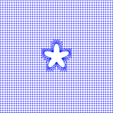
(a) Quadratic mesh before splitting elements near the boundary

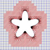
(b) AES-FEM boundary mesh after extraction and splitting

Figure 3: Example meshes before and after splitting near the boundary. In (b), the red linear triangles constitute the AES-FEM mesh, obtained by splitting quadratic elements.

4.5 Extension to Three Dimensions

While the process outlined in the paper is for 2D, we can extend this mesh generation method to 3D by addressing some additional challenges. First, unstructured mesh generation in 3D uses tetrahedra as the primary element shape. Superconvergent spectral elements, however, require the use of tensor-product elements, which, in 3D, have quadrilateral faces. To construct a conformal mesh, we must resolve the two boundaries by introducing pyramid-shaped elements, which cover the quadrilateral face boundary of the hexahedral mesh and the triangular boundary of the tetrahedral mesh. Meanwhile, the curved surface can be meshed using any standard surface mesh technique. The tetrahedral mesh generator meshes the space between the two boundaries. The fine-tuning for this part is determining the minimum distance from the pyramids’ boundary to ensure the stability of the tetrahedral mesh generation. Curvature in this context can be replaced by the maximum curvature Carmo1976 . More specifically, given a smooth parametric surface $S(u,v)\in\mathbb{R}^{2}\mapsto\mathbb{R}^{3}$, let $\boldsymbol{J}$ be the Jacobian matrix of $S$. We define the first fundamental matrix of $S$ as $\boldsymbol{G}=\boldsymbol{J}^{T}\boldsymbol{J}$. Since the vectors of the Jacobian matrix form a basis for the tangent space of the surface, we can define the normal direction of the surface as

$$\hat{\boldsymbol{n}}=\frac{S_{u}\times S_{v}}{\parallel S_{u}\times S_{v}\parallel}.$$

The second fundamental matrix is then defined as

$$\boldsymbol{B}=\left[\begin{array}[]{cc}\hat{\boldsymbol{n}}^{T}S_{uu}&\hat{\boldsymbol{n}}^{T}S_{uv}\\ \hat{\boldsymbol{n}}^{T}S_{vu}&\hat{\boldsymbol{n}}^{T}S_{vv}\end{array}\right].$$

The shape operator is then $\boldsymbol{W}=\boldsymbol{G}^{-1}\boldsymbol{B}$, of which the larger absolute value of its eigenvalues is the maximum curvature; the detailed computation can be found Wang2009 . We then use its inverse, namely the minimal radius of curvature, as the criteria for controlling the local edge lengths similar to the process outlined in section 4.2. As for the rest of the 2D algorithm, section 4.3 generalizes to 3D directly. We defer the implementation of 3D to future work, and we will focus on verifying the error analysis and the feasibility of the overall workflow in 2D.

5 Numerical Results

In this section, we present numerical results with our proposed method, primarily as a proof of concept in improving the numerical accuracy of SEM over curved domains. To this end, we solve the convection-diffusion equation

$$-\Delta u+\boldsymbol{v}\cdot\boldsymbol{\nabla}u=f \quad\text{on }\Omega,$$ (4)

$$u=u_{D} \quad\text{on }\Gamma_{D},$$ (5)

$$\partial_{\boldsymbol{n}}u=u_{N} \quad\text{on }\Gamma_{N},$$ (6)

where $f$ denotes a source term, and $u_{D}$ and $u_{N}$ denote the Dirichlet and Neumann boundary conditions, respectively. To assess accuracy, we used the method of manufactured solutions in 2D and computed $f$, $u_{D}$, and $u_{N}$ from the exact solution $u=\sin(10\pi x)\mathrm{cos}(10\pi y)+xy$ and $\boldsymbol{v}=[x,-y].$ We tested the method using two domains: a unit square centered at $(0.5,0.5)$ with an elliptical hole and a five-petal flower hole, respectively, as illustrated in Figure 4. For the elliptical hole, the semi-major and semi-minor axes are 0.2 and 0.1, respectively. The five-petal flower is a variant of the flower-shaped domain in cheung2019optimally , with the parametric equations

$$x= (0.25+0.1\sin(5\theta))\cos(\theta)/3+0.5$$

$$y= (0.25+0.1\sin(5\theta))\sin(\theta)/3+0.5$$

for $0\leq\theta<2\pi$. This domain is particularly challenging due to its high curvature and mixed convex-and-concave regions.

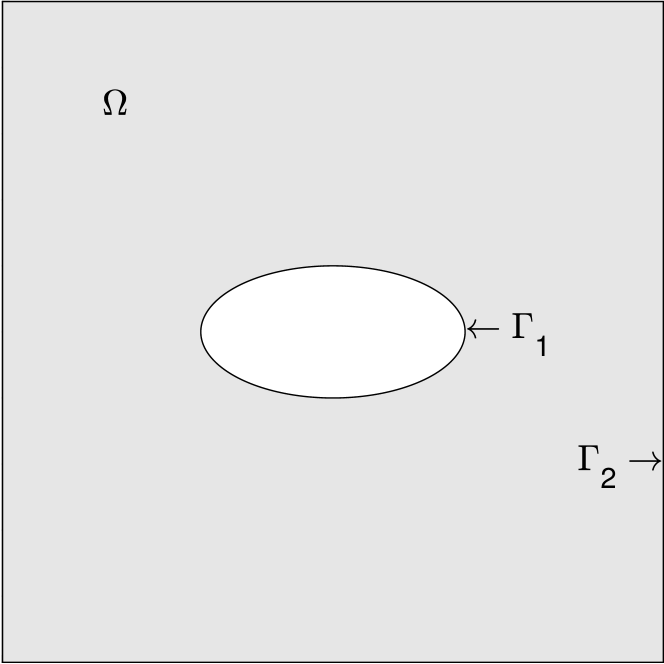
(a) Unit square with elliptical hole

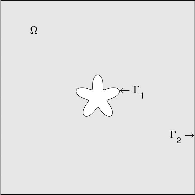
(b) Unit square with five-petal flower hole

Figure 4: Domains used in tests. Neumann or Dirichlet boundary conditions are applied to interior boundary $\Gamma_{1}$; Dirichlet boundary conditions are applied to exterior boundary $\Gamma_{2}$.

To demonstrate superconvergence, we measure the errors in $\ell_{2}$ norm instead of $L_{2}$ norm because the latter is dominated by the interpolation error. More specifically, let $\boldsymbol{u}$ and $\hat{\boldsymbol{u}}$ denote the vectors containing the exact and numerical solutions at the nodes; the $\ell_{2}$-norm error is then computed as

$$\mathrm{error}=\|\boldsymbol{u}-\hat{\boldsymbol{u}}\|_{2}=\sqrt{\sum_{i}(u_{i}-\hat{u}_{i})^{2}}.$$

Since the elements near the boundaries are irregular, we compute the convergence rate based on the number of degrees of freedom (dof), i.e.,

$$\mathrm{convergence\>rate}=-\log\left(\frac{\mathrm{error\,of\,fine\,mesh}}{\mathrm{error\,of\,coarse\,mesh}}\right)\biggl{/}\log\left(\sqrt[d]{\frac{\mathrm{dof\,in\,fine\,mesh}}{\mathrm{dof\,in\,coarse\,mesh}}}\right),$$

where $d=2$ is the topological dimension of the mesh. This formula is consistent with the edge-length-based convergence rate for structured meshes for sufficiently fine meshes.

5.1 Effect of $h$-GR on Curved Neumann Boundaries

We first assess the effect of $h$-GR on curved Neumann boundaries. To this end, we solved the convection-diffusion equation (4) on the elliptical-hole and flower-hole meshes with Neumann boundary conditions on the curved boundary $\Gamma_{1}$ of the flower hole and Dirichlet boundary conditions on $\Gamma_{2}$, as illustrated in Figure 4(a) and (b), respectively. We solved the equation using isoparametric FEM and SEM with and without $h$-GR; we studied the effect of superparametric elements in section 5.2. Figure 5 shows the $\ell_{2}$-norm errors of the nodal solutions with and without $h$-GR for quadratic, cubic, and quartic FEM and SEM. For completeness, Figure 5 also shows the results after post-processing the near-boundary elements. Note that quadratic FEM and SEM are identical, so there is only one set of results for both.

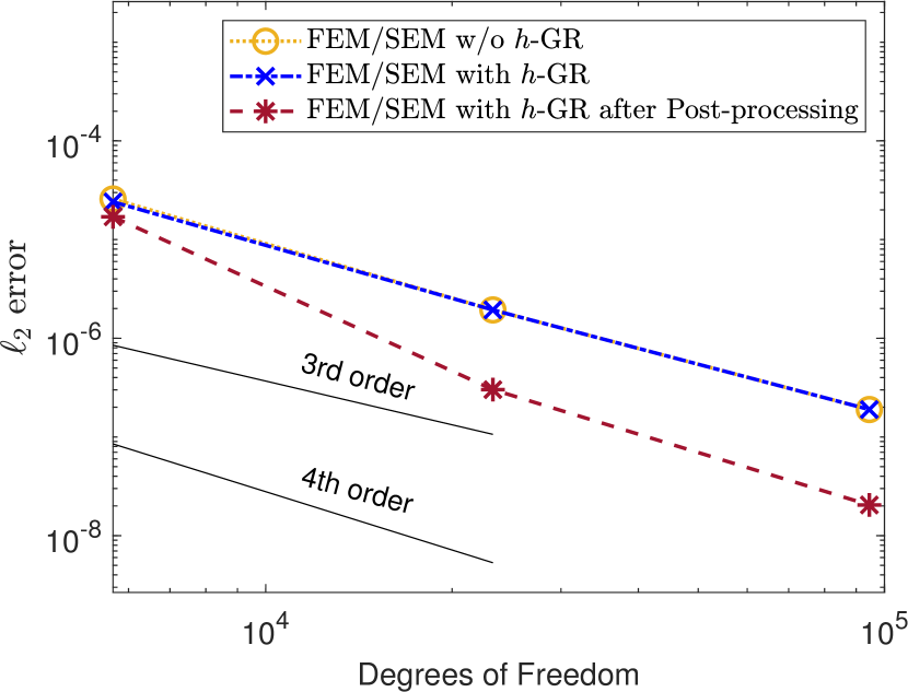
(a) Quadratic elliptical hole

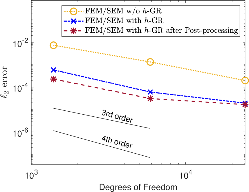
(b) Quadratic flower hole

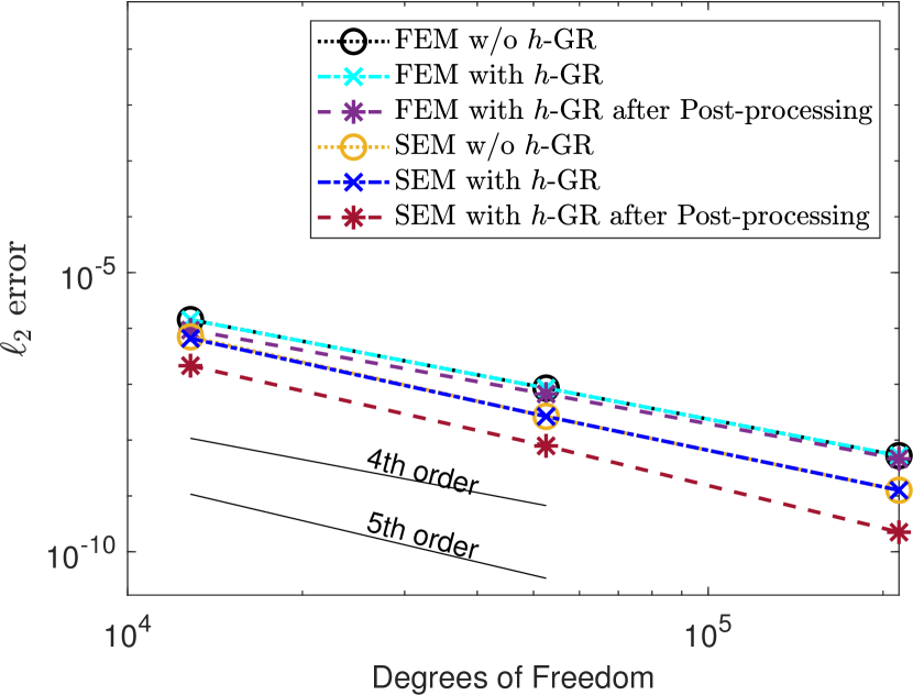
(c) Cubic elliptical hole

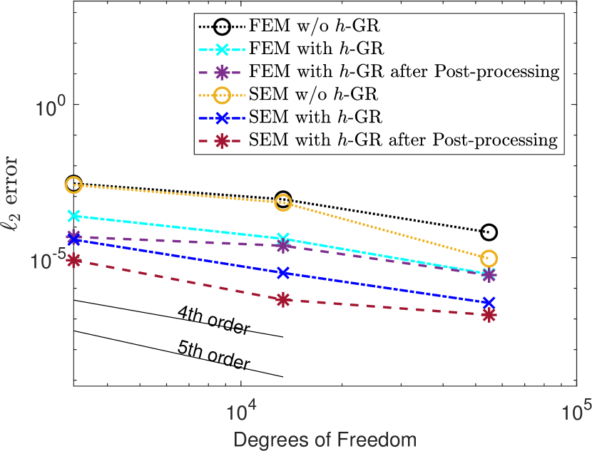
(d) Cubic flower hole

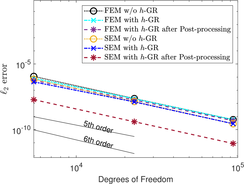
(e) Quartic elliptical hole

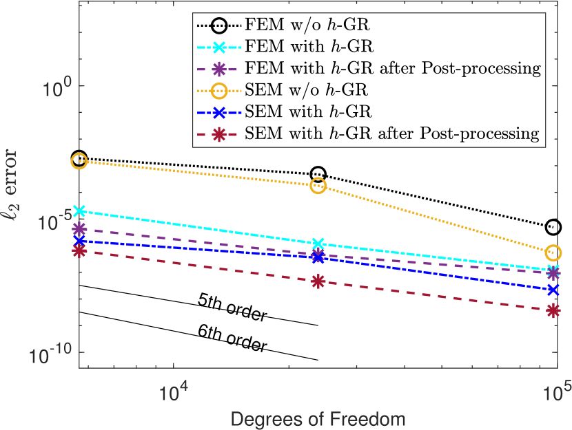
(f) Quartic flower hole

Figure 5: Comparison of nodal errors of spectral elements in the interior of the flower-hole domain with quadratic, cubic, and quartic SEM for the convection-diffusion equation with and without $h$-GR, as well as the error after post-processing.

From the results, we first observe that cubic and quartic SEM significantly outperformed their FEM counterparts in all cases. Hence, we will consider only SEM in our later discussions. We also observe that for the flower-hole mesh, $h$-GR alone improved the overall accuracy by about one, two, and three orders of magnitude for quadratic, cubic, and quartic SEM on the coarser and intermediate meshes. This drastic improvement is because $h$-GR improves the accuracy of the normal directions of high-curvature regions. The normals are implicitly used by Neumann boundary conditions in (3). In contrast, for the elliptical-hole mesh, $h$-GR alone did not improve accuracy much because the curvatures are not high for the ellipse, and the normals are reasonably accurate even without $h$-GR. Nevertheless, $h$-GR still improved the accuracy of the spectral elements near boundaries, even for the elliptical-hole domain. This improvement is evident because the post-processed SEM solution was significantly better with $h$-GR than without $h$-GR.

To gain more insights, we plotted $\ell_{2}$-norm errors of the nodal solutions of only the tensor-product spectral elements in the interior of the domain for the flower-hole mesh in Figure 6. It can be seen that curvature-based $h$-GR significantly improved the accuracy of SEM. These results also confirmed our analysis in section 3.1 that the geometric errors lead to significant pollution of the tensor-product elements in the interior of the domain. These improvements contribute to the majority of the improvements in Figure 5. Note that the improvements from $h$-GR alone started to plateau as the meshes were refined since the errors of near-boundary elements started to dominate, which were further reduced by our post-processing technique as shown in Figure 4.

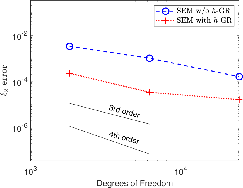
(a) Quadratic

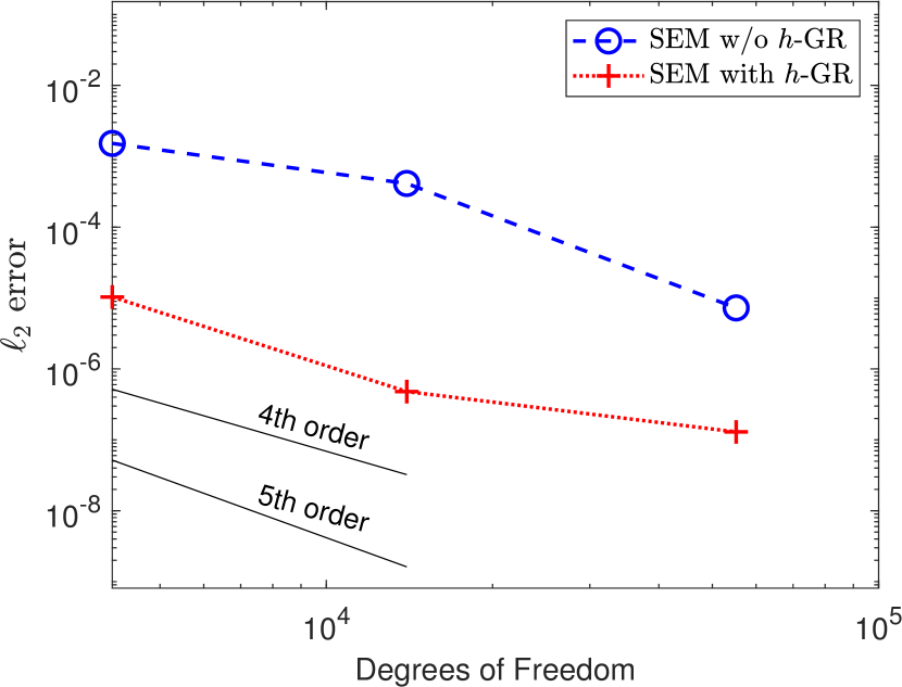
(b) Cubic

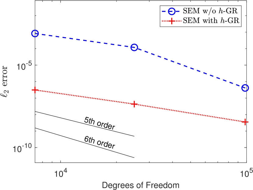
(c) Quartic

Figure 6: Comparison of nodal errors of spectral elements in the interior of the flower-hole domain with quadratic, cubic, and quartic SEM for the convection-diffusion equation with and without $h$-GR.

5.2 Effect of $p$-GR on Curved Neumann Boundaries

Next, we study the effect of superparametric elements ($p$-GR) on boundary elements. Similar to section 5.1, we solved the convection-diffusion equation (4) on both the elliptical-hole and flower-hole meshes with Neumann and Dirichlet boundary conditions on $\Gamma_{1}$ and $\Gamma_{2}$, respectively. However, this time we compare the error using isoparametric elements versus superparametric elements near the curved boundary $\Gamma_{1}$ for meshes with $h$-GR. Figure 7 shows the $\ell_{2}$-norm errors for both $h$-GR and $hp$-GR using SEM before and after post-processing. Here we omit the results with $p$-GR only, since it may increase the error if the curved boundary is under-resolved.

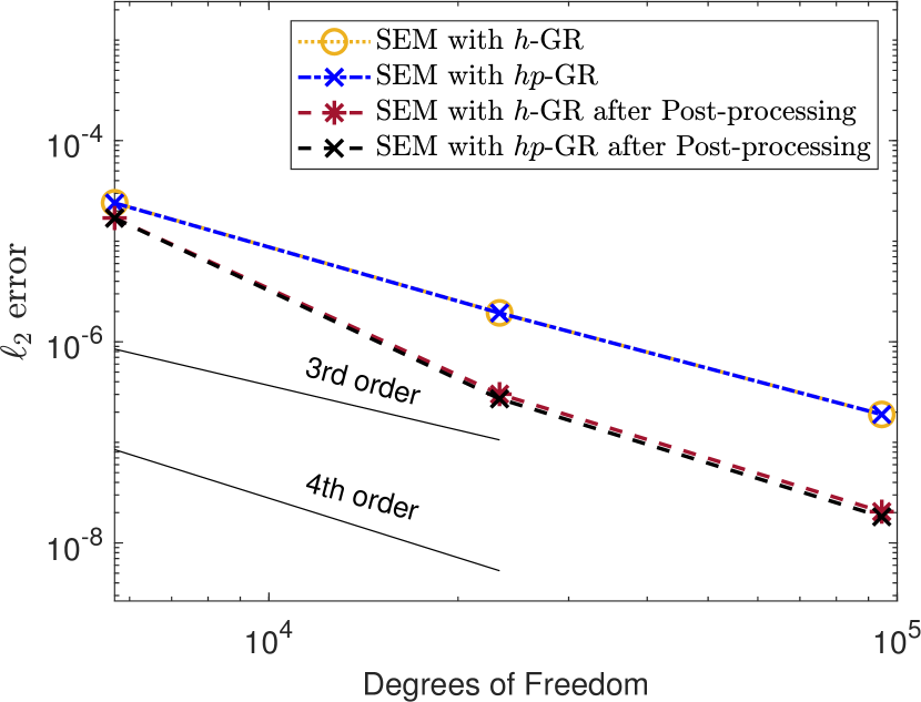
(a) Quadratic elliptical hole

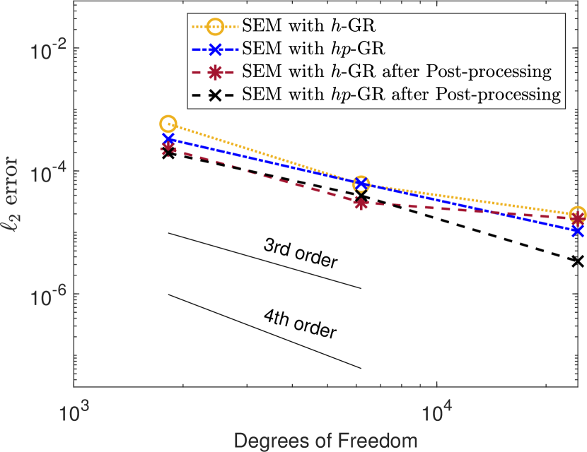
(b) Quadratic flower hole

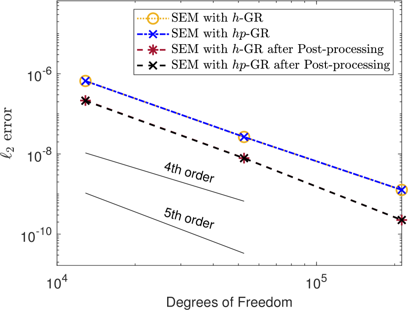
(c) Cubic elliptical hole

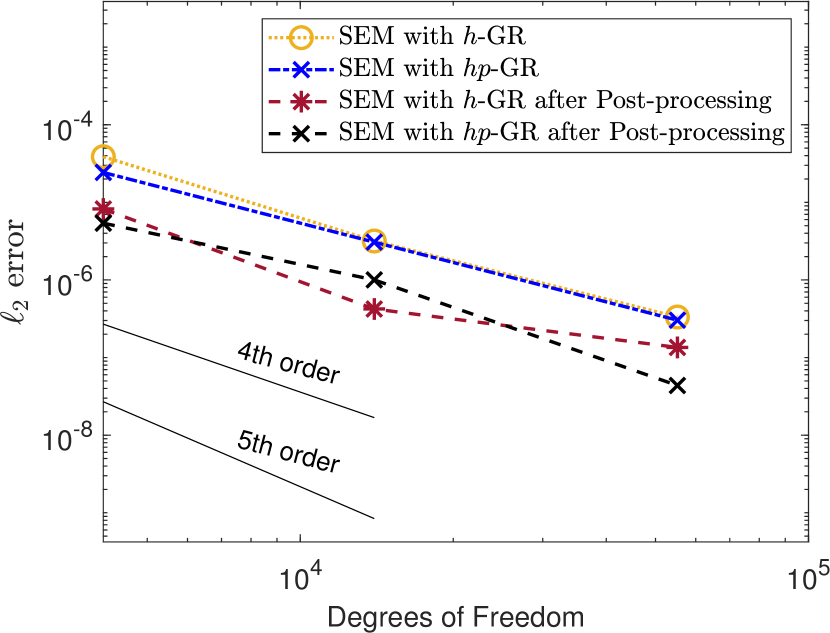
(d) Cubic flower hole

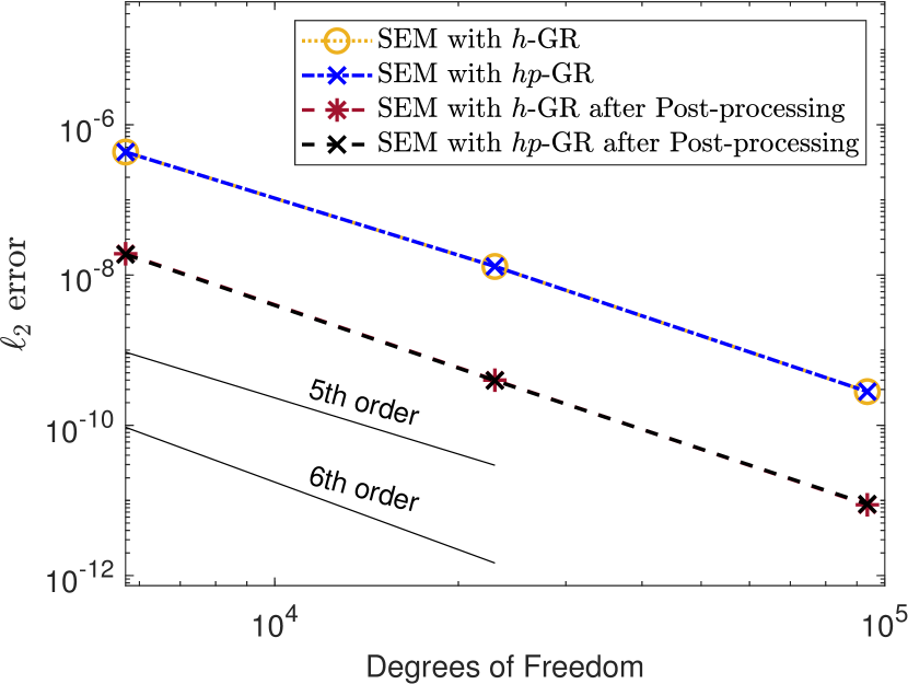
(e) Quartic elliptical hole

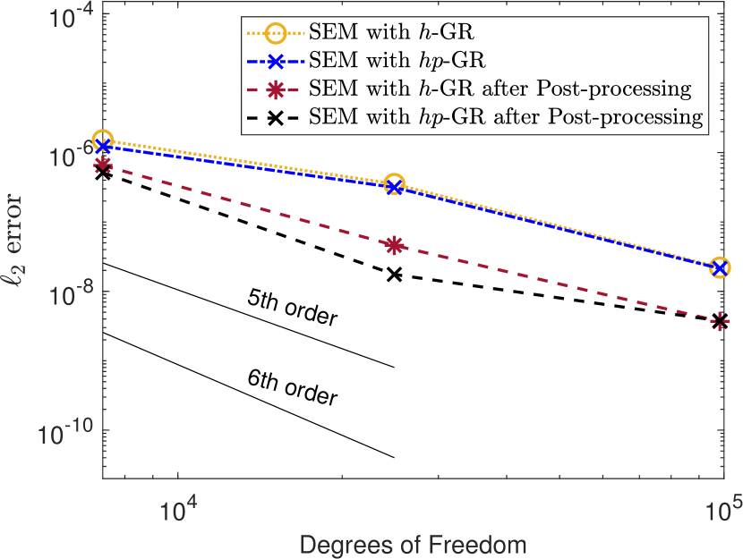
(f) Quartic flower hole

Figure 7: A comparison isoparametric elements versus superparametric elements ($h$-GR vs $hp$-GR) for the convection-diffusion equation on both the elliptical hole domain on the left side and the flower hole domain on the right with Dirichlet boundary conditions on the straight boundaries and Neumann boundary conditions on the curved boundaries solved with quadratic, cubic, and quartic SEM as well as the error after post-processing.

From the results, we observe that in a similar fashion to section 5.1, $hp$-GR improved the geometric accuracy of normals, reducing the error when using Neumann boundary conditions. However, the effect of going from $h$-GR to $hp$-GR is much less dramatic using SEM than from standard geometry to $h$-GR for the flower domain. The more significant results become clear after post-processing, in which superparametric elements can sometimes help recover superconvergence for domains with high curvature as presented in section 2.2. It has been theorized that isoparametric elements have sufficient geometric accuracy and that superparametric elements do not improve accuracy, in this regard. This result shows that when trying to recover $\ell_{2}$ superconvergence that was lost due to geometric inaccuracies near the boundary through post-processing, superparametric elements may be very useful by reducing the interpolation errors.

5.3 Accuracy Improvement for Curved Dirichlet Boundaries

In this subsection, we present the effect $h$-GR has using only Dirichlet boundary conditions on all boundaries of the meshes. Each graph contains the errors of SEM with and without $h$-GR as the errors after post-processing. Similar to the results in sections 5.1 and 5.2, we observe that increasing the geometric accuracy near a boundary with high curvature helps preserve the accuracy of superconvergent SEM in the interior after post-processing. Dirichlet boundary conditions, however, have some caveats in terms of how the geometric accuracy impacts the $\ell_{2}$ error. In contrast with nodes on Neumann boundary conditions, the nodes on a Dirichlet boundary have known function values, so the difference in adjacent normal derivatives does not play a role in the analysis. However, we do see that sufficient geometric accuracy is required to maintain high-order accuracy for interior elements after post-processing.

As shown in the left side of Figure 8, for the meshes with the elliptical hole, $h$-GR does not offer any advantages as standard meshes capture the true geometry close enough. For meshes with regions of high curvature, $h$-GR offers more advantages since meshes with $h$-GR better approximate the true geometry of the domain. From the right side of Figure 8, we can see that for coarse meshes with $h$-GR the accuracy of both the SEM and the post-processing solution are significantly better than the mesh without $h$-GR. The standard mesh can better approximate exact geometry for finer meshes, so the error is similar to using $h$-GR.

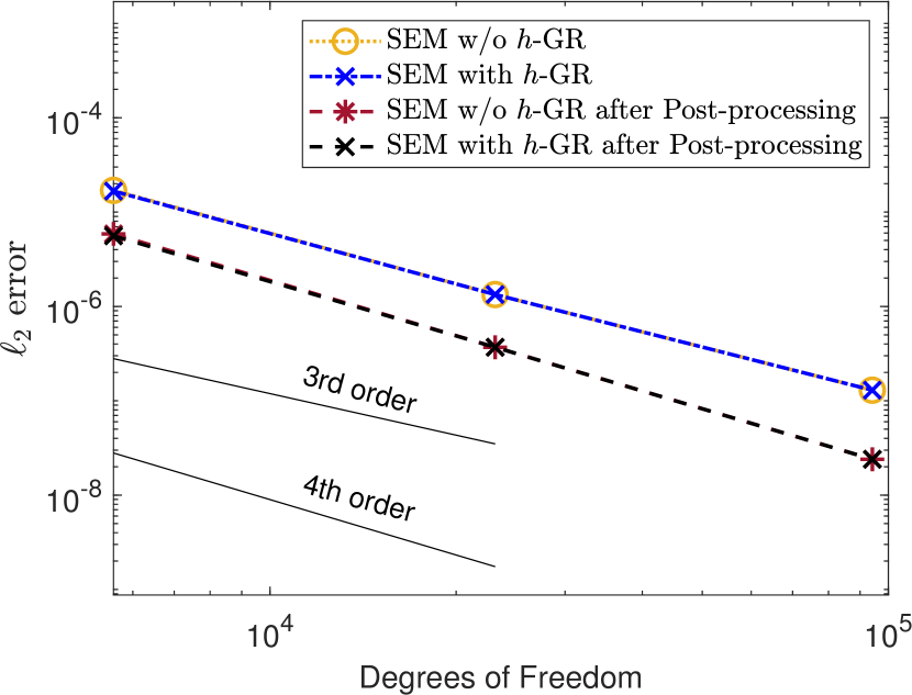
(a) Quadratic elliptical hole

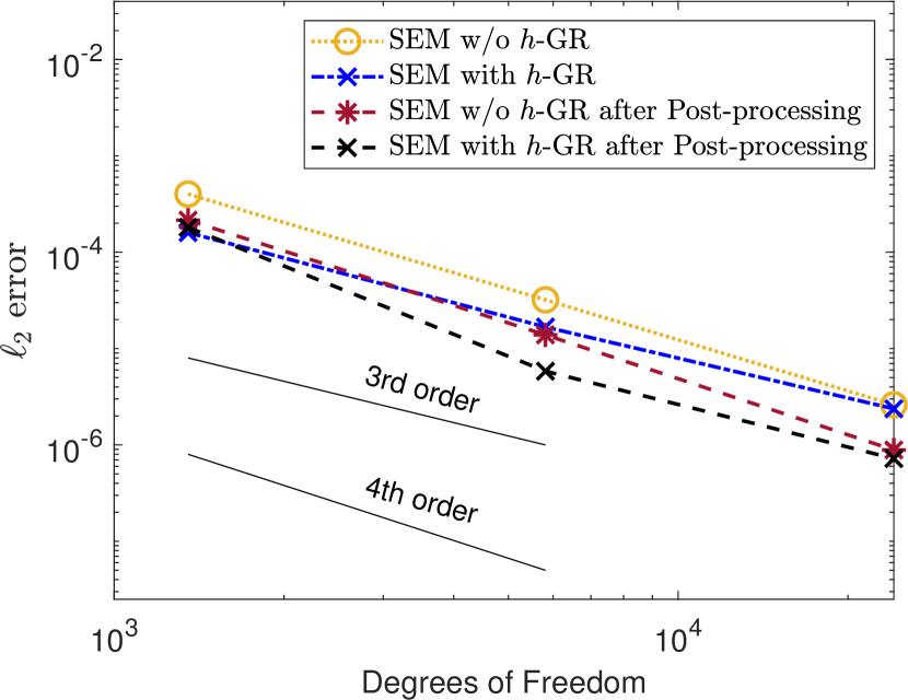
(b) Quadratic flower hole

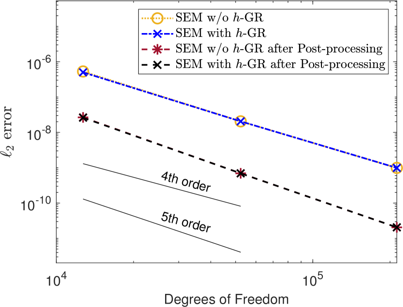
(c) Cubic elliptical hole

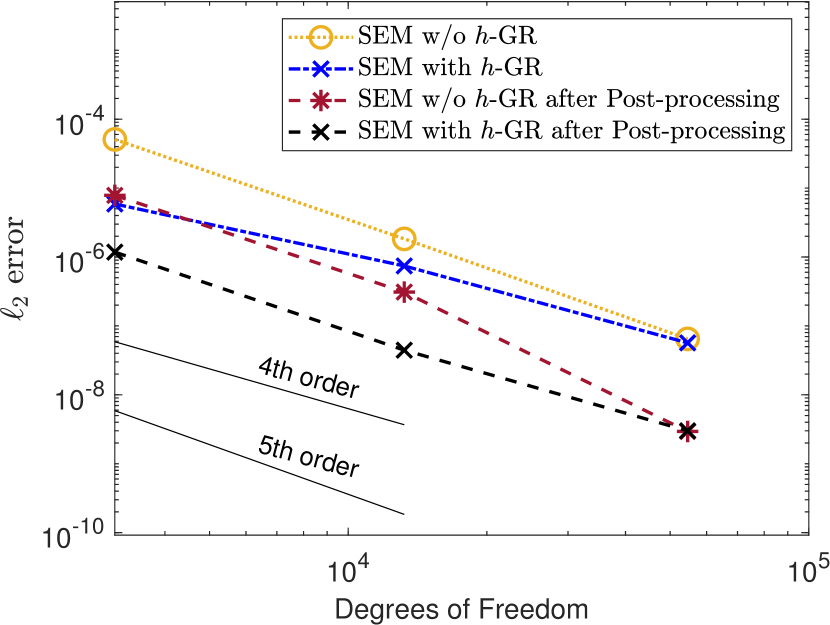
(d) Cubic flower hole

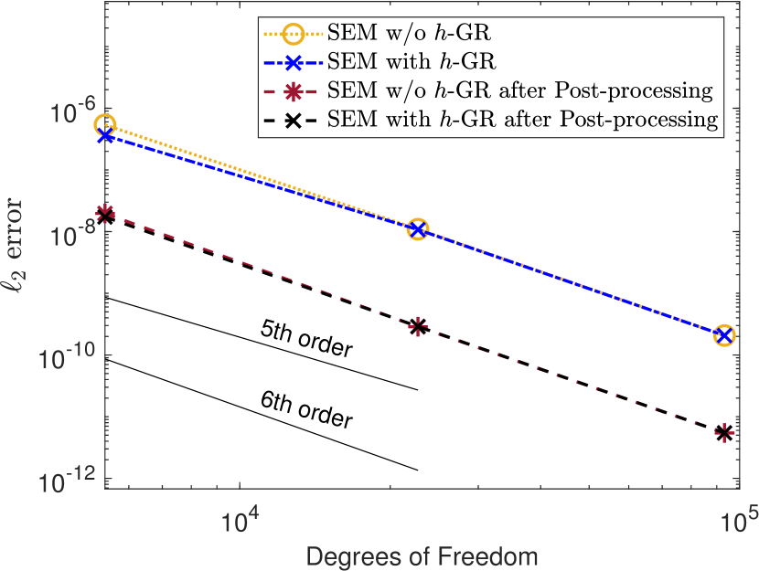
(e) Quartic elliptical hole

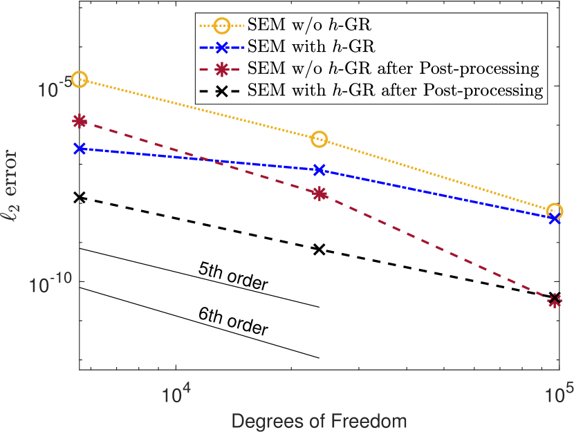
(f) Quartic flower hole

Figure 8: A comparison of isoparametric elements versus superparametric elements for the convection-diffusion equation on both the elliptical hole domain on the left side and the flower hole domain on the right with Dirichlet boundary conditions and quadratic, cubic, and quartic SEM, with $h$-GR as well as the error after post-processing.

5.4 Impact of Mesh Quality

Finally, we present the effect that mesh quality has on the $l_{2}$-error of meshes with and without $h$-GR, and the improvement of post-processing on the same meshes. Since we wanted to look at the effect geometric accuracy has on high curvatures, we will only use domain (b) from Figure 4. We manipulated the mesh quality by distorting a good quality mesh by moving several nodes such that the maximum angle among all elements is some specified degree $\theta.$ Specifically, we consider a series of meshes where the maximum angle is $180$ degrees minus $[10^{-4},10{}^{-3},10{}^{-2},10{}^{-1},10^{0},10{}^{1}]$ degrees. The results are shown in Figure 9, which plots the $l_{2}$-error on the $y$-axis and $180\text{°}$ minus the maximum angle on the $x$-axis. The figure inset shows the first three error values of SEM.

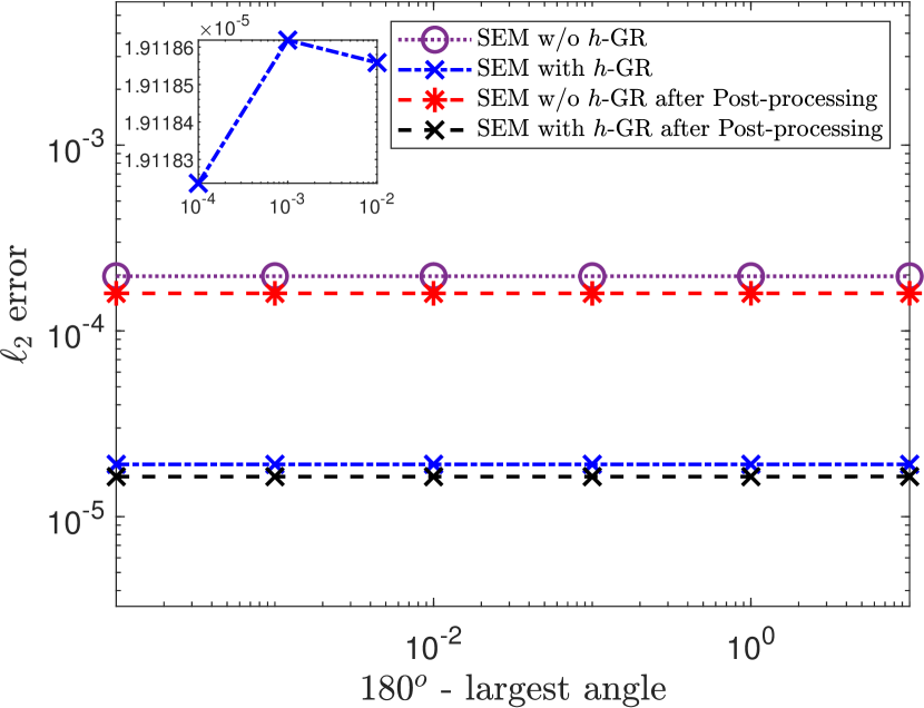
(a) Quadratic

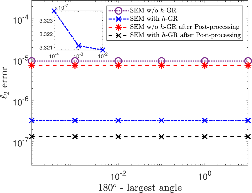
(b) Cubic

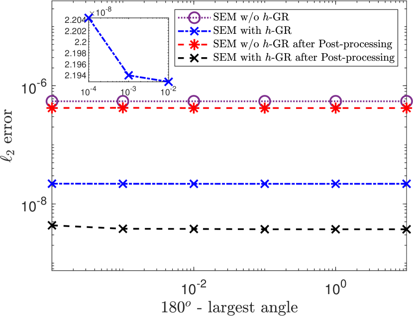
(c) Quartic

Figure 9: A mesh quality study which compares the errors of SEM and post-processing with and without $h$-GR. The horizontal axis shows the difference of $180\text{\textdegree}$ minus the largest angle in the mesh. The inset is a zoomed in version of the first three SEM errors.

First, we note that post-processing can improve the accuracy more as the order increases. We see this specifically as while post-processing meshes with $h$-GR improves the accuracy a little for the quadratic mesh, the quartic mesh enjoyed more than a ten-fold improvement in nodal error. This result is due to the improvement of geometric accuracy allowing for recovery of superconvergence as outlined in subsection 3.1. We also want to point out that meshes without $h$-GR do not improve much after post-processing, so superconvergence was lost. In Figure 9, we also show that $h$-GR and post-processing can reduce error significantly more than mesh quality optimization, provided that the maximum angle is less than $179.999\text{°}$, a relatively relaxed mesh generation requirement. These results suggest that $h$-GR and post-processing may greatly improve angle quality requirements for mesh generation and could reduce the meshing bottleneck significantly. Using AES-FEM near the boundary relaxes the dependency on element shapes. It will also ease the generalization to 3D, for which tetrahedral meshes are more prone to having poor-shaped elements (such as slivers) near boundaries.

6 Conclusions

In this paper, we introduced a novel approach to improve the accuracy of SEM over curved domains. Our approach utilizes mixed meshes with superconvergent tensor-product spectral elements in the interior of the domain and non-tensor-product elements (such as simplicial elements) near the boundary. We showed that $h$- and $p$-GR of near-boundary elements could substantially reduce the pollution errors to the spectral elements in the interior and preserve the superconvergence property of spectral elements. In addition, by utilizing AES-FEM to post-process the solutions near the boundary, we can make the accuracy of the non-tensor-product elements match those of the spectral elements. To the best of our knowledge, this work is the first to demonstrate superconvergence of SEM over curved domains. We showed that our proposed techniques could improve the accuracy of the overall solution by one to two orders of magnitude. At the same time, the element shapes have a substantially smaller impact on the accuracy. As a result, our proposed approach can substantially relax the mesh-quality requirement and, in turn, alleviate the burden of mesh generation for higher-order methods, especially near boundaries. We presented numerical results in 2D as proof of concept. Future work includes the implementation in 3D and optimization of the implementation.

Declarations

Conflict of interest

The authors have no relevant financial or non-financial interests to disclose.

References

- [1] I. Babuška and A. Miller. The post-processing approach in the finite element method-Part 1: calculation of displacements, stresses and other higher derivatives of the displacements. Int. J. Numer. Methods. Eng., 20(6):1085–1109, 1984.
- [2] F. Bassi and S. Rebay. High-order accurate discontinuous finite element solution of the 2D Euler equations. J. Comput. Phys., 138(2):251–285, 1997.
- [3] B. Boroomand and O. Zienkiewicz. An improved REP recovery and the effectivity robustness test. Int. J. Numer. Methods. Eng., 40(17):3247–3277, 1997.
- [4] B. Boroomand and O. C. Zienkiewicz. Recovery by equilibrium in patches (REP). Int. J. Numer. Methods. Eng., 40(1):137–164, 1997.
- [5] L. Botti and D. A. Di Pietro. Assessment of hybrid high-order methods on curved meshes and comparison with discontinuous Galerkin methods. J. Comput. Phys., 370:58–84, 2018.
- [6] J. H. Bramble and A. H. Schatz. Higher order local accuracy by averaging in the finite element method. Math. Comp., 31(137):94–111, 1977.
- [7] S. C. Brenner and C. Carstensen. Finite element methods. Comput. Mech., 1:73–114, 2004.
- [8] C. Chen. Orthogonality correction technique in superconvergence analysis. Int. J. Numer. Anal. Model., 2005(1):31–42, 2005.
- [9] C. Chen and S. Hu. The highest order superconvergence for bi-k degree rectangular elements at nodes: a proof of 2k-conjecture. Math. Comput., 82(283):1337–1355, 2013.
- [10] C. M. Chen. Superconvergence of finite element solutions and their derivatives. Numer. Math. J. Chinese. Univ., 3(2):118–125, 1981.
- [11] C. M. Chen. Superconvergence for triangular finite elements. Science in China Series A: Mathematics, 42(9):917–924, 1999.
- [12] C. M. Chen and Y. Q. Huang. High Accuracy Theory of Finite Elements (in Chinese). Hunan Science and Technique Press, Changsha, 1995.
- [13] J. Cheung, M. Perego, P. Bochev, and M. Gunzburger. Optimally accurate higher-order finite element methods for polytopial approximations of domains with smooth boundaries. Math. Comput., 88(319):2187–2219, 2019.
- [14] P. G. Ciarlet and P.-A. Raviart. The combined effect of curved boundaries and numerical integration in isoparametric finite element methods. In The Mathematical Foundations of the Finite Element Method with Applications to Partial Differential Equations, pages 409–474. Elsevier, 1972.
- [15] R. Conley, T. J. Delaney, and X. Jiao. Overcoming element quality dependence of finite elements with adaptive extended stencil FEM (AES-FEM). Int. J. Numer. Methods. Eng., 108(9):1054–1085, 2016.
- [16] R. Conley, T. J. Delaney, and X. Jiao. A hybrid method and unified analysis of generalized finite differences and lagrange finite elements. J. Comput. Appl. Math., 376:112862, 2020.
- [17] F. Dassi, A. Mola, and H. Si. Curvature-adapted remeshing of CAD surfaces. Procedia. Eng., 82:253–265, 2014.
- [18] M. do Carmo. Differential Geometry of Curves and Surfaces. Prentice-Hall, 1976.
- [19] V. Dyedov, N. Ray, D. Einstein, X. Jiao, and T. Tautges. AHF: Array-based half-facet data structure for mixed-dimensional and non-manifold meshes. Eng. Comput., 31:389–404, 2015.
- [20] M. R. Eslami. Finite Elements Methods in Mechanics. Springer, 2014.
- [21] B. A. Finlayson. The Method of Weighted Residuals and Variational Principles. SIAM, 2013.
- [22] T. J. Hughes, J. A. Cottrell, and Y. Bazilevs. Isogeometric analysis: CAD, finite elements, NURBS, exact geometry and mesh refinement. Comput. Methods. Appl. Mech. Eng., 194(39-41):4135–4195, 2005.
- [23] X. Jiao, D. Wang, and H. Zha. Simple and effective variational optimization of surface and volume triangulations. Eng. Comput., 27:81–94, 2011.
- [24] G. Karniadakis and S. Sherwin. Spectral/hp Element Methods for Computational Fluid Dynamics. OUP Oxford, 2005.
- [25] D. Khan, A. Plopski, Y. Fujimoto, M. Kanbara, G. Jabeen, Y. J. Zhang, X. Zhang, and H. Kato. Surface remeshing: A systematic literature review of methods and research directions. IEEE. Trans. Vis. Comput. Graph., 28(3):1680–1713, 2020.
- [26] D. Komatitsch, R. Martin, J. Tromp, M. A. Taylor, and B. A. Wingate. Wave propagation in 2-D elastic media using a spectral element method with triangles and quadrangles. J. Comput. Acoust., 9(02):703–718, 2001.
- [27] M. Křížek and P. Neittaanmäki. On superconvergence techniques. Acta. Appl. Math., 9:175–198, 1987.
- [28] Y. Li, X. Zhao, N. Ray, and X. Jiao. Compact feature-aware hermite-style high-order surface reconstruction. Eng. Comput., 37(1):187–210, 2021.
- [29] S. Lloyd. Least squares quantization in PCM. IEEE. Trans. Inf. Theory., 28(2):129–137, 1982.
- [30] X. Luo, M. S. Shephard, and J.-F. Remacle. The influence of geometric approximation on the accuracy of high order methods. Rensselaer SCOREC report, 1, 2001.
- [31] Y. Maday and E. M. Rønquist. Optimal error analysis of spectral methods with emphasis on non-constant coefficients and deformed geometries. Comput. Methods. Appl. Mech. Eng., 80(1-3):91–115, 1990.
- [32] S. Mansouri and H. Ebrahimnezhad. Segmentation-based semi-regular remeshing of 3D models using curvature-adapted subdivision surface fitting. J. Vis., 19:141–155, 2016.
- [33] D. Moxey, M. Green, S. Sherwin, and J. Peiró. An isoparametric approach to high-order curvilinear boundary-layer meshing. Comput. Methods. Appl. Mech. Eng., 283:636–650, 2015.
- [34] A. Naga and Z. Zhang. A Posteriori error estimates based on the polynomial preserving recovery. SIAM. J. Numer. Anal., 42(4):1780–1800, 2004.
- [35] A. T. Patera. A spectral element method for fluid dynamics: laminar flow in a channel expansion. J. Comput. Phys., 54(3):468–488, 1984.
- [36] M. A. Scott, M. J. Borden, C. V. Verhoosel, T. W. Sederberg, and T. J. Hughes. Isogeometric finite element data structures based on Bézier extraction of T-splines. Int. J. Numer. Methods. Eng., 88(2):126–156, 2011.
- [37] R. Sevilla, S. Fernández-Méndez, and A. Huerta. NURBS-enhanced finite element method (NEFEM). Int. J. Numer. Methods. Eng., 76(1):56–83, 2008.
- [38] R. Sevilla, S. Fernández-Méndez, and A. Huerta. Comparison of high-order curved finite elements. Int. J. Numer. Methods. Eng., 87(8):719–734, 2011.
- [39] G. Strang and G. Fix. An Analysis of the Finite Element Method. Prentice-Hall, 1973.
- [40] M. A. Taylor, B. A. Wingate, and R. E. Vincent. An algorithm for computing Fekete points in the triangle. SIAM. J. Numer. Anal., 38(5):1707–1720, 2000.
- [41] The CGAL Project. CGAL User and Reference Manual. CGAL Editorial Board, 5.5.2 edition, 2023.
- [42] The MathWorks Inc. Partial differential equation toolbox version: 9.4 (R2022b), 2022.
- [43] D. Wang, B. Clark, and X. Jiao. An analysis and comparison of parameterization-based computation of differential quantities for discrete surfaces. Comput. Aided. Geom. Des., 26(5):510–527, 2009.
- [44] Q. Zhu. A review of two different approaches for superconvergence analysis. Appl. Math., 43(6):401–411, 1998.
- [45] O. C. Zienkiewicz and J. Zhu. The superconvergent patch recovery (SPR) and adaptive finite element refinement. Comput. Methods. Appl. Mech. Eng., 101(1-3):207–224, 1992.
- [46] M. Zlámal. Superconvergence and reduced integration in the finite element method. Math. Comput., 32(143):663–685, 1978.
- [47] M. Zlàmal. Some superconvergence results in the finite element method. In Mathematical Aspects of Finite Element Methods: Proceedings of the Conference Held in Rome, December 10–12, 1975, pages 353–362. Springer, 2006.
- [48] P. Zwanenburg and S. Nadarajah. On the necessity of superparametric geometry representation for discontinuous galerkin methods on domains with curved boundaries. In 23rd AIAA Computational Fluid Dynamics Conference, page 3946, 2017.