The Nonlocal Neural Operator:
Universal Approximation

Abstract

Neural operator architectures approximate operators between infinite-dimensional Banach spaces of functions. They are gaining increased attention in computational science and engineering, due to their potential both to accelerate traditional numerical methods and to enable data-driven discovery. A popular variant of neural operators is the Fourier neural operator (FNO). Previous analysis proving universal operator approximation theorems for FNOs resorts to use of an unbounded number of Fourier modes and limits the basic form of the method to problems with periodic geometry. Prior work relies on intuition from traditional numerical methods, and interprets the FNO as a nonstandard and highly nonlinear spectral method. The present work challenges this point of view in two ways: (i) the work introduces a new broad class of operator approximators, termed nonlocal neural operators (NNOs), which allow for operator approximation between functions defined on arbitrary geometries, and includes the FNO as a special case; and (ii) analysis of the NNOs shows that, provided this architecture includes computation of a spatial average (corresponding to retaining only a single Fourier mode in the special case of the FNO) it benefits from universal approximation. It is demonstrated that this theoretical result unifies the analysis of a wide range of neural operator architectures. Furthermore, it sheds new light on the role of nonlocality, and its interaction with nonlinearity, thereby paving the way for a more systematic exploration of nonlocality, both through the development of new operator learning architectures and the analysis of existing and new architectures.

1 Introduction

1.1 Motivation and Literature Review

Neural networks (Goodfellow et al., 2016) are receiving growing interest in computational science and engineering. In many applications of interest in the sciences, the task at hand is to approximate an underlying operator, which defines a mapping between two infinite-dimensional Banach spaces of functions. New neural network-based frameworks, termed neural operators (Anandkumar et al., 2020; Bhattacharya et al., 2021; Lu et al., 2021; Kovachki et al., 2021a), generalize neural networks to this infinite-dimensional setting, with the aim of learning such operators from data. They have the potential to accelerate traditional numerical methods when a mathematical description, often in the form of a partial differential equation, is known. When no model is available, this data-driven methodology has the potential to discover the underlying input-output map.

Several neural operator architectures have been proposed in recent years. The first neural operator architecture (i) appeared in Chen and Chen (1995) and was subsequently generalized by adding a depth component to the underlying networks (DeepONet) (Lu et al., 2021); further extensions include (Jin et al., 2022; Seidman et al., 2022; Lanthaler et al., 2022; Patel et al., 2022). DeepONets have been successfully deployed in a variety of application areas (Di Leoni et al., 2021; Mao et al., 2021; Cai et al., 2021). Concurrently with DeepONet a number of other approaches to operator learning have also been developed and successfully deployed including: (ii) methods which combine ideas from principal component analysis with neural networks (PCA-Net) Hesthaven and Ubbiali (2018); Bhattacharya et al. (2021); (iii) operator learning based on random features, which may be viewed as Monte Carlo approximation of kernel methods, as introduced in (Nelsen and Stuart, 2021); and (iv) the wide class of neural operators introduced in (Anandkumar et al., 2020; Kovachki et al., 2021a). The class of methods (iv) defines neural operators in analogy with conventional neural networks, but appends the weight matrices in the hidden layers with additional linear integral operators acting on the input function. Special cases of this framework include graph neural operators (Anandkumar et al., 2020; Li et al., 2020) and the Fourier neural operator (FNO) (Li et al., 2021a). The FNO in particular has received considerable interest due to its state-of-the-art performance on many tasks. The FNO, and extensions thereof, remains a very active research direction: see, for example, (Wen et al., 2022; Li et al., 2022; You et al., 2022; Pathak et al., 2022; Li et al., 2021b). We also mention the closely related convolutional neural operator of Raonić et al. (2023). The reliance on a Fourier basis limits the basic form of the FNO to periodic geometries although, in that setting, use of the fast Fourier transform (FFT) allows for efficient computations with total number of Fourier components limited only by the grid resolution. There is a set of papers which seek to address the restriction to periodic geometry by replacing the FFT with a wavelet Tripura and Chakraborty (2023) or multi-wavelet Gupta et al. (2021) transform; in this context, we also mention the Laplace neural operator Chen et al. (2023). The Laplace neural operator does not use the Laplace transform; the terminology refers to generalizing the FNO to use arbitrary orthogonal eigenfunctions of the Laplace operator on any given spatial domain. Another approach to extending the scope of the FFT is to learn transformations of arbitrary domains into unit cubes, suitable for application of the FFT Li et al. (2022). Most closely related to the approach proposed in the present paper is the low rank neural operator (Kovachki et al., 2021a, Sect. 4.2) which, however, has a more complicated architecture than that proposed here.

There is a growing body of approximation theory for certain classes of operators arising from PDEs, using Galerkin and Taylor approximation in high dimensional spaces; see (Cohen and DeVore, 2015; Kaarnioja et al., 2023) for recent overviews of this literature, in particular in the context of the Darcy flow problem as pioneered in the paper Cohen et al. (2010). However the empirical success of neural operators on very wide classes of operator learning problems, beyond those covered by classical approximation theoretic approaches, suggests the value of developing theory for neural operators. A prerequisite for the success of any neural operator architecture, and its use in a diverse range of applications, is a universal approximation property. Universal approximation results are known for DeepONets (Chen and Chen, 1995; Lanthaler et al., 2021), PCA-Net (Bhattacharya et al., 2021), for general neural operators (Kovachki et al., 2021a) and for the (more constrained) Fourier neural operator (Kovachki et al., 2021b). As most operators of interest are not only nonlinear, but also nonlocal, any successful operator learning framework must share both of these properties. While the need for nonlinearity is well-understood even for ordinary neural networks, nonlocality is a requirement that is more specific to the function-space setting; it is a crucial ingredient for operator learning. The headline message of this paper is that universal approximation can be obtained in general geometries, with nonlocality introduced using only a low-rank operator of fixed finite rank, and is not restricted to periodic domains.

Fourier neural operators introduce nonlocality via the addition of a nonlocal operator in each hidden layer, which acts on the Fourier modes of the input function by matrix multiplication. Available analysis of FNOs in Kovachki et al. (2021b) mostly rests on an analogy between FNOs and spectral methods: higher approximation accuracy is established by retaining larger numbers of Fourier modes. This interpretation is at odds with practical experience with FNOs. FNOs are typically implemented with a first layer which lifts the input, a scalar or vector-valued function, to a vector-valued function where the vector dimension (referred to as the number of channels, also named the model width) is much higher than that of the input function itself. In some circumstances it can be more beneficial to increase the number of channels rather to retain more Fourier modes in the architecture. A first theoretical insight into this empirical observation has recently been achieved in (Lanthaler et al., 2022) from the perspective of nonlinear reconstruction, where the analysis of specific settings revealed clear benefits of increasing the number of channels, and showed that, in those specific cases, arbitrary accuracy can be achieved when retaining only a fixed number of Fourier modes; the same paper also contains numerical experiments which exemplify the theoretical insight. These and similar results indicate that our theoretical understanding of neural operators, which has been largely guided by experience with traditional numerical methods, is still incomplete, and suggests a need for further analysis to improve our understanding of the precise role of nonlocality in operator learning.

These observations motivate the present work. We introduce the nonlocal neural operator (NNO), a new class of operator approximators which include the FNO as a special case, but which apply to mappings between functions defined on domains with arbitrary geometries. We provide two universal approximation theorems for the NNO, both shedding new light on the role of nonlocality, and its interplay with nonlinearity, in operator learning. As a byproduct, the analysis provides an improved understanding of the benefits of increasing the number of channels, rather than the number of Fourier modes, in the FNO architecture. At a more fundamental level, and underlying this concrete problem, we achieve a deeper understanding of “how much” nonlocality is needed in neural operator architectures. The surprising result of the present work is that even very simple nonlocality, in the form of an integral average, is already sufficient for universality in operator learning. This is astonishing if one contrasts the simplicity of a humble average with the often incredibly complex nonlocal operators of interest in engineering and the sciences, which, for example, give rise to turbulence and other complex phenomena. The present work thus paves the way for a more systematic exploration of nonlocality in operator learning.

In the next subsection we introduce the NNO, and state two universal approximation theorems for it. This subsection summarizes the key contributions of the paper. In section 2 we introduce a key analysis tool: the averaging neural operator (ANO). We state, and sketch the proof of, two universal approximation theorems; proof details are given in the Appendix A. The ANO is a subclass of the NNO, but also of numerous other neural operators, including many of those listed in the preceding literature review; we thus deduce, in section 3, many universal approximation theorems, including those for the NNO, from properties of the ANO. We follow this, in section 4, with numerical experiments illustrating some of the implications of our work. Section 5 contains concluding discussions.

1.2 Nonlocal Neural Operator

We now introduce the following nonlocal neural operator (NNO) architecture. Let $\Omega$ denote a bounded domain in $\mathbb{R}^{d}$ and let $\mathcal{X}(\Omega;\mathbb{R}^{o}),\mathcal{Y}(\Omega;\mathbb{R}^{o})$ and $\mathcal{V}(\Omega;\mathbb{R}^{o})$ denote Banach spaces of $\mathbb{R}^{o}-$valued functions over $\Omega.$ The NNO is defined as a mapping $\Psi:\mathcal{X}(\Omega;\mathbb{R}^{k})\to\mathcal{Y}(\Omega;\mathbb{R}^{k^{\prime}})$ which can be written as a composition of the form $\Psi=\mathcal{Q}\circ\mathcal{L}_{L}\circ\dots\circ\mathcal{L}_{1}\circ\mathcal{R}$, consisting of a lifting layer $\mathcal{R}$, hidden layers $\mathcal{L}_{\ell}$, $\ell=1,\dots,L$, and a projection layer $\mathcal{Q}$. Given a channel dimension ${d_{c}}$, the lifting layer $\mathcal{R}$ is given by a mapping

$$\mathcal{R}:\mathcal{X}(\Omega;\mathbb{R}^{k})\to\mathcal{V}(\Omega;\mathbb{R}^{d_{c}}),\quad u(x)\mapsto R(u(x),x),$$ (1.1)

where $R:\mathbb{R}^{k}\times\Omega\to\mathbb{R}^{d_{c}}$ is a learnable neural network acting between finite dimensional Euclidean spaces. For $\ell=1,\dots,L$ (the number of hidden layers) and for $m=0,\dots,M$ (the number of modes) choose functions $\psi_{\ell,m},\phi_{\ell,m}:\Omega\to\mathbb{R}^{d_{c}}$. For $\ell=1,\dots,L$, each hidden layer $\mathcal{L}_{\ell}$ is of the form

$$(\mathcal{L}_{\ell}v)(x):=\sigma\left(W_{\ell}v(x)+b_{\ell}+\sum_{m=0}^{M}\langle T_{\ell,m}v,\psi_{\ell,m}\rangle_{L^{2}(\Omega;\mathbb{R}^{d_{c}})}\phi_{\ell,m}(x)\right).$$ (1.2)

Each hidden layer defines a mapping $\mathcal{L}_{\ell}:\mathcal{V}(\Omega;\mathbb{R}^{d_{c}})\to\mathcal{V}(\Omega;\mathbb{R}^{d_{c}}).$ For $\ell=1,\dots,L$ and for $m=0,\dots,M$ the matrices $W_{\ell},T_{\ell,m}\in\mathbb{R}^{{d_{c}}\times{d_{c}}}$, and bias $b_{\ell}\in\mathbb{R}^{d_{c}}$ are learnable parameters. The activation function $\sigma:\mathbb{R}\to\mathbb{R}$ acts as a Nemitskii-operator, component-wise on inputs; i.e. for a vector-valued function $v(x)=(v_{1}(x),\dots,v_{d_{c}}(x))$, we define $\sigma(v(x)):=(\sigma(v_{1}(x)),\dots,\sigma(v_{d_{c}}(x)))$ for $x\in\Omega$. Throughout the paper the activation function $\sigma:\mathbb{R}\to\mathbb{R}$ is assumed to be smooth, $\sigma\in C^{\infty}(\mathbb{R})$, nonpolynomial and Lipschitz continuous. Finally, the projection layer $\mathcal{Q}$ is given by a mapping,

$$\mathcal{Q}:\mathcal{V}(\Omega;\mathbb{R}^{d_{c}})\to\mathcal{Y}(\Omega;\mathbb{R}^{k^{\prime}}),\quad v(x)\mapsto Q(v(x),x),$$ (1.3)

where $Q:\mathbb{R}^{{d_{c}}}\times\Omega\to\mathbb{R}^{k^{\prime}}$ is also a learnable neural network acting between finite dimensional Euclidean spaces.

The proposed architecture opens up new potential applications which will benefit from the empirical success of the FNO, but not be limited by geometry. However, it reduces to the FNO in a periodic geometry and if the modes are chosen as Fourier basis functions, indexed by $m$ and independent of $\ell.$ The NNO architecture comes with universal approximation theorems, two of which we now state. As corollaries, these theorems apply to the FNO and establish that the FNO is a universal approximator with a fixed number of Fourier modes. In the following, we set ${\bf{1}}=(1,\dots,1)^{\top}\in\mathbb{R}^{d_{c}}.$

Theorem 1.1.

Let $\Omega\subset\mathbb{R}^{d}$ be a bounded domain with Lipschitz boundary. For given integers $s,s^{\prime}\geq 0$, let $\Psi^{\dagger}:C^{s}(\overline{\Omega};\mathbb{R}^{k})\to C^{s^{\prime}}(\overline{\Omega};\mathbb{R}^{k^{\prime}})$ be a continuous operator, and fix a compact set $\mathsf{K}\subset C^{s}(\overline{\Omega};\mathbb{R}^{k})$. Assume that for all $\ell=1,\dots,L$, we have $\psi_{\ell,0}\equiv\phi_{\ell,0}\equiv{\bf{1}}$, the vector-valued constant function. Then with any fixed choice of integers $L\geq 1$ and $M\geq 0$, and for arbitrary $\epsilon>0$, there exists a nonlocal neural operator $\Psi:\mathsf{K}\subset C^{s}(\overline{\Omega};\mathbb{R}^{k})\to C^{s^{\prime}}(\overline{\Omega};\mathbb{R}^{k^{\prime}})$ with the approximation property

$$\sup_{u\in\mathsf{K}}\|\Psi^{\dagger}(u)-\Psi(u)\|_{C^{s^{\prime}}}\leq\epsilon.$$

The key observation here is that $L$ and $M$ are fixed; the universal approximation is achieved by increasing the number of channels $d_{c}.$ Theorem 1.1 is a corollary of Theorem 2.1 showing that in fact $L=1,M=0$ suffices for the theory (though is unlikely to be optimal in practice). The previous result is formulated for operators on spaces of continuously differentiable functions. However, it is possible to obtain similar results in many other natural settings. To illustrate the generality of the underlying ideas, we provide a corresponding result in the scale of Sobolev spaces $W^{s,p}$; the following is a corollary of Theorem 2.2.

Theorem 1.2.

Let $\Omega\subset\mathbb{R}^{d}$ be a bounded domain with Lipschitz boundary. For given integers $s,s^{\prime}\geq 0$, and reals $p,p^{\prime}\in[1,\infty)$, let $\Psi^{\dagger}:W^{s,p}(\Omega;\mathbb{R}^{k})\to W^{s^{\prime},p^{\prime}}(\Omega;\mathbb{R}^{k^{\prime}})$ be a continuous operator. Fix a compact set $\mathsf{K}\subset W^{s,p}(\Omega;\mathbb{R}^{k})$ of bounded functions: $\sup_{u\in K}\|u\|_{L^{\infty}}<\infty$. Assume that for all $\ell=1,\dots,L$, we have $\psi_{\ell,0}\equiv\phi_{\ell,0}\equiv{\bf{1}}$, the vector-valued constant function. Then with any fixed choice of integers $L\geq 1$ and $M\geq 0$, and for arbitrary $\epsilon>0$, there exists a nonlocal neural operator $\Psi:W^{s,p}(\Omega;\mathbb{R}^{k})\to W^{s^{\prime},p^{\prime}}(\Omega;\mathbb{R}^{k^{\prime}})$ with the approximation property

$$\sup_{u\in\mathsf{K}}\|\Psi^{\dagger}(u)-\Psi(u)\|_{W^{s^{\prime},p^{\prime}}}\leq\epsilon.$$

2 Averaging Suffices for Universal Approximation

In this section we prove that the use of a simple average provides enough nonlocality, within the broader NNO structure, leading to the two universal approximation Theorems 2.1 and 2.2 stated below. The architecture used to prove these theorems is a subclass of the NNO architecture, and hence implies the two universal approximation Theorems 1.1 and 1.2 as corollaries. When the domain is periodic, the resulting neural operator is also a special case of the FNO, when only the zeroth Fourier mode is retained. Thus, our universality result also implies the universality of FNOs, even when only computing with a single, constant, Fourier mode. Thus the theoretical results in this section provide new insight into the empirical observation, for example in the experiments in (Lanthaler et al., 2022), that increasing the number of channels is often more beneficial than increasing the number of Fourier modes in the practical training of FNOs. In subsection 2.1 we discuss the nonlinearity of neural networks between finite dimensional Euclidean spaces and emphasize the role of nonlocality in operator learning. Subsection 2.2 defines the subclass of NNOs used for our analysis of universal approximation, the topic of subsection 2.3. The proof is sketched in subsection 2.4, with details left for the appendix.

2.1 Nonlinearity and Nonlocality

To achieve a universal approximation property, a neural operator architecture must necessarily define a nonlinear operator. In the context of ordinary neural networks acting as approximators of functions between finite dimensional Euclidean spaces, it is well-known that (nonpolynomial) nonlinearity essentially also represents a sufficient condition for their universal approximation property (Pinkus, 1999; Barron, 1993; Hornik et al., 1989; Cybenko, 1989). This should be contrasted with neural operators, where nonlinearity alone is not sufficient to ensure universality; to illustrate this latter fact, we note that even a single layer of an ordinary neural network actually gives rise to a nonlinear operator, which maps an input function to an output function by composition,

$$u(x)\mapsto\sigma(Wu(x)+b).$$ (2.1)

Here, $W$ and $b$ represent the weights and biases, respectively, and $\sigma$ denotes the activation function. Despite being highly nonlinear, operators of such a compositional form cannot be universal. The main reason for this is that any such $\Psi$ is local, in the sense that the value $\Psi(u)(x)$ of the output function at a given evaluation point $x$ depends only on the value of the input function $u(x)$ at that same evaluation point. As a consequence, such mappings are not able to approximate even simple operators $\Psi^{\dagger}$ with a nonlocal dependency on the input, such as the shift operator $\Psi^{\dagger}(u)(x):=u(x+h)$ for fixed $h\neq 0$.

The arguably simplest example of a nonlocal operator with dependency on all point values $u(x)$, $x\in\Omega$, is given by averaging the input function $u$ over its domain $\Omega$:

$$u(x)\mapsto\fint_{\Omega}u(y)\,dy:=\frac{1}{|\Omega|}\int u(y)\,dy.$$ (2.2)

Clearly, such averaging represents only a very special case of a nonlocal operator. In general, nonlocal operators can have a much more complicated dependence on the function values ${\left\{u(x)\,\middle|\,x\in\Omega\right\}}$ over the whole domain, as well as the mutual correlations of these values.

2.2 Averaging Neural Operator: a Special Subclass of the NNO

In this section, we define a special subclass of the NNO, which combines nonlinearity by composition (2.1) with nonlocality by averaging (2.2). Recall that we have restricted this paper to consideration of only smooth, nonpolynomial and Lipschitz continuous activation functions $\sigma$. Generalization of our results to other activation functions is possible, but would require additional technical assumptions in our main results. We now define the subclass of NNOs found by simplifying to a special subclass of hidden layers of the form,

$$\mathcal{L}_{\ell}:\mathcal{V}(\Omega;\mathbb{R}^{d_{c}})\to\mathcal{V}(\Omega;\mathbb{R}^{d_{c}}),\quad\mathcal{L}_{\ell}(v)(x):=\sigma\left(W_{\ell}v(x)+b_{\ell}+\fint_{\Omega}v(y)\,dy\right).$$ (2.3)

We refer to this specific subclass of the NNO as the averaging neural operator (ANO). The ANO thus depends on two hyperparameters; the depth $L$ and the lifting dimension ${d_{c}}$. The tunable parameters of an averaging neural operator are represented by the weights $W_{\ell}\in\mathbb{R}^{{d_{c}}\times{d_{c}}}$ and biases $b_{\ell}\in\mathbb{R}^{{d_{c}}}$ across the hidden layers, and the internal weights and biases of the ordinary neural networks $R$ and $Q$, which define the lifting and projection layers, respectively.

2.3 Universal Approximation

Despite the apparent simplicity of averaging as the only nonlocal ingredient in the definition of the averaging neural operator, the following theorem shows that this architecture is universal:

Theorem 2.1.

Let $\Omega\subset\mathbb{R}^{d}$ be a bounded domain with Lipschitz boundary. For given integers $s,s^{\prime}\geq 0$, let $\Psi^{\dagger}:C^{s}(\overline{\Omega};\mathbb{R}^{k})\to C^{s^{\prime}}(\overline{\Omega};\mathbb{R}^{k^{\prime}})$ be a continuous operator, and fix a compact set $\mathsf{K}\subset C^{s}(\overline{\Omega};\mathbb{R}^{k})$. Then for any $\epsilon>0$, there exists an averaging neural operator $\Psi:\mathsf{K}\subset C^{s}(\overline{\Omega};\mathbb{R}^{k})\to C^{s^{\prime}}(\overline{\Omega};\mathbb{R}^{k^{\prime}})$ such that

$$\sup_{u\in\mathsf{K}}\|\Psi^{\dagger}(u)-\Psi(u)\|_{C^{s^{\prime}}}\leq\epsilon.$$

The previous result is formulated for operators on spaces of continuously differentiable functions. However, it is possible to obtain similar results in many other natural settings. To illustrate the generality of the underlying ideas, we provide a corresponding result in the scale of Sobolev spaces $W^{s,p}$:

Theorem 2.2.

Let $\Omega\subset\mathbb{R}^{d}$ be a bounded domain with Lipschitz boundary. For given integers $s,s^{\prime}\geq 0$, and reals $p,p^{\prime}\in[1,\infty)$, let $\Psi^{\dagger}:W^{s,p}(\Omega;\mathbb{R}^{k})\to W^{s^{\prime},p^{\prime}}(\Omega;\mathbb{R}^{k^{\prime}})$ be a continuous operator. Fix a compact set $\mathsf{K}\subset W^{s,p}(\Omega;\mathbb{R}^{k})$ of bounded functions, $\sup_{u\in K}\|u\|_{L^{\infty}}<\infty$. Then for any $\epsilon>0$, there exists an averaging neural operator $\Psi:W^{s,p}(\Omega;\mathbb{R}^{k})\to W^{s^{\prime},p^{\prime}}(\Omega;\mathbb{R}^{k^{\prime}})$ such that

$$\sup_{u\in K}\|\Psi^{\dagger}(u)-\Psi(u)\|_{W^{s^{\prime},p^{\prime}}}\leq\epsilon.$$

The two preceding theorems have, as respective corollaries, Theorems 1.1 and 1.2.

2.4 Sketch Of The Proof Of Universality

In the present section, we provide an overview of the proof of Theorems 2.1 and 2.2. The details are included in Appendix A, see Sections A.5 and A.6, in particular. In the following overview, let $\mathcal{X}=\mathcal{X}(\Omega;\mathbb{R}^{k})$ and $\mathcal{Y}=\mathcal{Y}(\Omega;\mathbb{R}^{k^{\prime}})$ denote spaces of continuously differentiable functions (respectively Sobolev spaces) as in the statement of Theorem 2.1 (respectively Theorem 2.2).

The first step in the proof of universality is to determine a reduction to a special class of operators, explained in detail in Section A.3, which have the structure of an encoder-decoder. Starting from a general continuous operator $\Psi^{\dagger}:\mathcal{X}\to\mathcal{Y}$, and given a compact set $\mathsf{K}\subset\mathcal{X}$, we first show that for any $\epsilon>0$, there exist $J\in\mathbb{N}$, elements $\eta_{1},\dots,\eta_{J}\in\mathcal{Y}$ and continuous functionals $\alpha_{1},\dots,\alpha_{J}:\mathcal{X}\to\mathbb{R}$, such that

$$\sup_{u\in\mathsf{K}}\left\|\Psi^{\dagger}-\sum_{j=1}^{J}\alpha_{j}(u)\eta_{j}\right\|_{\mathcal{Y}}\leq\epsilon.$$ (2.4)

Furthermore, our construction ensures that each of these functionals $\alpha_{j}$ actually defines a continuous functional on the larger input function space consisting of $L^{1}$-functions, i.e. we have continuous mappings $\alpha_{j}:L^{1}(\Omega;\mathbb{R}^{k})\to\mathbb{R}$. Since any input function space $\mathcal{X}$ considered in Theorems 2.1 and 2.2 embeds into $L^{1}(\Omega;\mathbb{R}^{k})$, this first step in the proof reduces the original problem to the approximation of a continuous operator $\widetilde{\Psi}^{\dagger}:L^{1}(\Omega;\mathbb{R}^{k})\to\mathcal{Y}$, of the form,

$$\widetilde{\Psi}^{\dagger}(u)=\sum_{j=1}^{J}\alpha_{j}(u)\eta_{j},$$ (2.5)

over a compact subset $\mathsf{K}\subset L^{1}(\Omega;\mathbb{R}^{k})$ of uniformly bounded functions, $\sup_{u\in K}\|u\|_{L^{\infty}}<\infty$. The structure of $\widetilde{\Psi}$ is that of an encoder-decoder, with the functionals $\alpha_{j}$ providing the encoding and the functions $\phi_{j}$ the decoding. We refer to Proposition A.3 for further details in the setting of continuously differentiable spaces, and Proposition A.3 for a corresponding statement in the scale of Sobolev spaces.

The second step in the proof, described in detail in Section A.4, concerns approximation of the continuous nonlinear functionals $\alpha_{j}:L^{1}(\Omega;\mathbb{R}^{k})\to\mathbb{R}$, the encoders. Specifically, we show that they can be approximated to any desired accuracy $\epsilon$ by an averaging neural operator $\widetilde{\alpha}:L^{1}(\Omega;\mathbb{R}^{k})\to\mathbb{R}^{J}$ (with constant output functions), and with components $\widetilde{\alpha}(u)=(\widetilde{\alpha}_{1}(u),\dots,\widetilde{\alpha}_{J}(u))$. To be concrete,

$$\sup_{u\in\mathsf{K}}\left|\alpha_{j}(u)-\widetilde{\alpha}_{j}(u)\right|\leq\epsilon,\quad\forall\,j=1,\dots,J.$$

This result is contained in Lemma A.4 of Section A.4, which constitutes the main ingredient in the proof of universality. More precisely, the constructed averaging neural operator $\widetilde{\alpha}$ is of the form

$$\widetilde{\alpha}:u\mapsto R(u(x),x)\mapsto v:=\sigma\left(\fint_{\Omega}R(u(y),y)\,dy\right)\mapsto q_{1}(v),$$

where $R:\mathbb{R}^{k}\times\Omega\to\mathbb{R}^{d_{c}}$ and $q_{1}:\mathbb{R}^{d_{c}}\to\mathbb{R}^{J}$ are ordinary neural networks; see Remark A.4 after the proof of Lemma A.4. This step builds on well-known approximation results for ordinary neural networks, summarized in Section A.2, and combines them with an averaging operation.

The final third step in the proof of Theorem 1.1 is given in Section A.5 (see p. A.5) and is built on approximations of the functions $\phi_{j}$ which define the decoder. We first show that there exists another (ordinary) neural network $q_{2}:\mathbb{R}^{J}\times\Omega\to\mathbb{R}^{k^{\prime}}$, such that $q_{2}(v,x)\approx\sum_{j=1}^{J}v_{j}\eta_{j}(x)$ for all relevant $(v,x)$, approximating the decoding. We then define a neural network $Q$ by the composition $Q(v,x):=q_{2}(q_{1}(v),x)$.

Given the neural network $R$ and averaging layer $\mathcal{L}(u):=\sigma\left(\fint_{\Omega}w(y)\,dy\right)$ from step two of the proof, and the neural network $Q$ from step three, we show that the averaging neural operator $\Psi:L^{1}(\Omega;\mathbb{R}^{k})\to\mathcal{Y}$, given by the composition,

$$\Psi:u(x)\overset{\mathcal{R}}{\mapsto}R(u(x),x)\overset{\mathcal{L}}{\mapsto}v:=\sigma\left(\fint_{\Omega}R(u(y),y)\,dy\right)\overset{\mathcal{Q}}{\mapsto}Q(v,x),$$ (2.6)

approximates the encoder-decoder (2.5). Concretely, given any $\epsilon>0$, we may design the neural networks $R$ and $Q$ so that

$$\sup_{u\in\mathsf{K}}\left\|\Psi(u)-\sum_{j=1}^{J}\alpha_{j}(u)\eta_{j}\right\|_{\mathcal{Y}}\leq\epsilon.$$

Step one of the proof shows that an encoder-decoder can be constructed to $\epsilon-$approximate the true map $\Psi^{\dagger}$, as stated in (2.4). It thus follows that averaging neural operators are universal approximators of general continuous operators $\Psi^{\dagger}:\mathcal{X}\to\mathcal{Y}$.

Two important properties of $\mathcal{X}$ and $\mathcal{Y}$ that are used in this proof are that (a) $\mathcal{X}$ has a continuous embedding in $L^{1}(\Omega;\mathbb{R}^{k})$, and (b) that functions $\eta_{1},\dots,\eta_{J}\in\mathcal{Y}(\Omega;\mathbb{R}^{k^{\prime}})$ can be approximated by ordinary neural networks, i.e. for any $\epsilon>0$, there exist neural networks $\widetilde{\eta}_{1},\dots,\widetilde{\eta}_{J}:\Omega\to\mathbb{R}^{k^{\prime}}$, such that $\|\eta_{j}-\widetilde{\eta}_{j}\|_{\mathcal{Y}}\leq\epsilon$. In addition, a more technical ingredient for the reduction to an operator of the form (2.5) is the existence of a “mollification”, defining a family of maps $\mathcal{M}_{\delta}:L^{1}(\Omega;\mathbb{R}^{k})\to\mathcal{X}$, and satisfying $\|\mathcal{M}_{\delta}u-u\|_{\mathcal{X}}\to 0$ as $\delta\to 0$, for any $u\in\mathcal{X}\subset L^{1}$. Relevant mathematical background, including a result on boundary-adapted mollification, is summarized in Appendix A.1. For simplicity of exposition, rather than striving for the greatest generality, we have formulated our universal approximation theorem for two concrete families of function spaces, $C^{s}$ and $W^{s,p}$, which satisfy the required properties and which cover most settings encountered in applications.

We note that additional properties, such as boundary conditions, are often implicitly enforced, provided that the operator is approximated with respect to a suitable norm on the output function space. For example, if the output functions belong to the Sobolev space $W^{1,2}_{0}(\Omega;\mathbb{R}^{k^{\prime}})$, respecting a homogeneous Dirichlet boundary condition, then approximation of the operator with respect to the $W^{1,2}(\Omega;\mathbb{R}^{k^{\prime}})$-norm automatically ensures that the boundary conditions are at least approximately satisfied, as a consequence of the trace theorem (Evans, 2010, Sect. 5.5).

In the outline above, the parameter $J$ directly relates to the required width of the network $Q$ defining the projection layer $\mathcal{Q}$. Thus, $J$ can be interpreted as a measure of the complexity of the output function space. The channel dimension ${d_{c}}$ corresponds to the number of necessary “features”, encoded via the components $\sigma\left(\fint_{\Omega}R_{1}(u(y),y)\,dy\right),\dots,\sigma\left(\fint_{\Omega}R_{d_{c}}(u(y),y)\,dy\right)$ of the composition $\mathcal{L}\circ\mathcal{R}$, needed to approximate the functionals $\alpha_{j}$ to a given accuracy. These nonlinear features provide an encoding of the input function, and ${d_{c}}$ is a measure of the information content that needs to be retained.

A careful look at the proof of Theorem 1.1 and Theorem 1.2, summarized above, reveals that a single averaging layer $\mathcal{L}$ is in fact enough to ensure universality of the resulting architecture, as can be seen from (2.6). As mentioned before, the mapping $\mathcal{L}\circ\mathcal{R}:\mathcal{X}\to\mathbb{R}^{d_{c}}$, $u\mapsto\mathcal{L}\circ\mathcal{R}(u)$ can be thought of as a nonlinear encoding of the input function by a (constant) vector $v\in\mathbb{R}^{d_{c}}$, while the mapping $\mathcal{Q}:\mathbb{R}^{d_{c}}\to\mathcal{Y}$, $v\mapsto Q(v,{\,\cdot\,})$ is a nonlinear decoding of the corresponding output function $\Psi^{\dagger}(u)$. This encoder/decoder perspective provides further insight as to why the universal approximation property can hold even when relying on simple averaging.

Given the last remark, our derivation actually implies that neural operators of the form (2.6) are universal in approximating continuous operators $\Psi^{\dagger}:\mathcal{X}(\Omega;\mathbb{R}^{k})\to\mathcal{Y}(\Omega^{\prime};\mathbb{R}^{k^{\prime}})$ on distinct domains $\Omega\subset\mathbb{R}^{d}$ and $\Omega^{\prime}\subset\mathbb{R}^{d^{\prime}}$, and with potentially different dimensions $d\neq d^{\prime}$. We only need to replace $Q$ in (2.6) by a neural network mapping $Q^{\prime}:\mathbb{R}^{d_{c}}\times\Omega\to\mathbb{R}^{k^{\prime}}$. The input and output spaces $\mathcal{X},\mathcal{Y}$ can be any combination of $C^{s}(\overline{\Omega};\mathbb{R}^{k}),W^{s,p}(\Omega;\mathbb{R}^{k})$ and $C^{s^{\prime}}(\overline{\Omega}^{\prime};\mathbb{R}^{k^{\prime}}),W^{s^{\prime},p^{\prime}}(\Omega^{\prime};\mathbb{R}^{k^{\prime}})$, respectively, for any integers $s,s^{\prime}\geq 0$ and reals $p,p^{\prime}\in[1,\infty)$.

3 Connection With Other Neural Operator Architectures

In this section we discuss the implications of the work in the previous section for, and links with, other neural operator architectures. Several neural operator architectures can be viewed as generalizations of the ANO, and a specific choice of the weights in the hidden layers will reproduce the simple averaging considered in the present work. Examples include the Fourier neural operator, the wavelet neural operator and neural operator with general integral kernel. As a consequence, the universal approximation property for the ANO immediately implies corresponding universal approximation results for these architectures. Furthermore, there are links to emerging and existing neural operator architectures such as the Laplace neural operator, DeepONet and NOMAD. We now detail these implications and links.

3.1 Neural Operator With General Integral Kernel

Recall that the hidden layers of an ANO are of the form

$$\mathcal{L}_{\ell}(v)(x)=\sigma\left(W_{\ell}v(x)+b_{\ell}+(\mathcal{K}_{\ell}v)(x)\right),$$ (3.1)

where $\mathcal{K}_{\ell}$ is the nonlocal operator given by averaging, $\mathcal{K}_{\ell}v=\fint_{\Omega}v(y)\,dy$. This is a special case of the general form of neural operators defined in Kovachki et al. (2021a) (General Neural Operator), where the hidden layers are of the form (3.1), with nonlocal operator given by integration against a matrix-valued integral kernel $K_{\ell}(x,y)\in\mathbb{R}^{{d_{c}}\times{d_{c}}}$:

$$(\mathcal{K}_{\ell}v)(x)=\int_{\Omega}K_{\ell}(x,y)v(y)\,dy.$$ (3.2)

The particular choice $K_{\ell}(x,y)\equiv|\Omega|^{-1}I_{{d_{c}}\times{d_{c}}}$ with $I_{{d_{c}}\times{d_{c}}}$ the identity matrix, recovers the ANO. Hence, as an immediate consequence of the universal approximation theorems 1.1 and 1.2, we obtain:

[General Neural Operator] The neural operator architecture with general integral kernel is universal in the settings of Theorem 2.1 and Theorem 2.2. This result generalizes the universal approximation theorem of Kovachki et al. (2021a) to even more general input and output spaces.

3.2 Low-Rank Neural Operator

A particular choice of the general integral kernel (3.2), proposed in (Kovachki et al., 2021a, Sect. 4.2), leads to the low-rank neural operator. Here, the integral kernel $K_{\ell}(x,y)$ of each layer is expanded in the low-rank form,

$$K_{\ell}(x,y)=\sum_{k=1}^{r}\phi_{\ell,j}(x)\psi_{\ell,j}(y)^{T},$$

where $\phi_{\ell,j},\psi_{\ell,j}:\Omega\to\mathbb{R}^{d_{c}}$ are vector-valued functions determined by neural networks, and optimized during the training of the low-rank neural operator. If $r={d_{c}}$, and choosing the neural networks to be constant, $\phi_{\ell,j}\equiv|\Omega|^{-1}e_{j}$, $\psi_{\ell,j}\equiv e_{j}$ with $e_{j}\in\mathbb{R}^{d_{c}}$ the $j$-th unit vector, we obtain $K_{\ell}(x,y)=|\Omega|^{-1}I_{{d_{c}}\times{d_{c}}}$. This recovers the ANO. Thus, we conclude: [Low-Rank Neural Operator] The neural operator architecture with low-rank kernel with $r\geq{d_{c}}$ is universal in the settings of Theorem 2.1 and Theorem 2.2.

Note that the NNO proposed in the present work differs from what is proposed in (Kovachki et al., 2021a, Sect. 4.2): here we pre-specify the functions $\phi_{\ell,j},\psi_{\ell,j}$, and learn only a multiplier; in contrast, the pre-existing work proposed learning these functions as neural networks. In this sense, the NNO can be viewed as a special case of the low-rank neural operator.

3.3 Fourier Neural Operator

The Fourier neural operator is obtained by restricting to a class of convolutional integral kernels in (3.2), i.e. kernels satisfying $K_{\ell}(x,y)=K_{\ell}(x-y)$, where $K_{\ell}(x)$ is a trigonometric polynomial of the form $K_{\ell}(x)=\sum_{|k|\leq k_{\mathrm{max}}}\widehat{P}_{\ell,k}e^{ikx}$ with $\widehat{P}_{\ell,k}\in\mathbb{C}^{{d_{c}}\times{d_{c}}}$. Upon setting $\ell=1$, $k_{\mathrm{max}}=0$, and $\widehat{P}_{1,0}=|\Omega|^{-1}I_{{d_{c}}\times{d_{c}}}$, we again recover the averaging neural operator. Thus, Theorem 2.1 immediately implies: [Fourier Neural Operator] The Fourier neural operator architecture is universal in the settings of Theorem 2.1 and Theorem 2.2. This result generalizes the previous universal approximation theorem of Kovachki et al. (2021b) to arbitrary Sobolev input and output spaces.

3.4 Wavelet Neural Operator

Multi-wavelet neural operators have been introduced in Gupta et al. (2021); see also Tripura and Chakraborty (2023). Following the approach in Gupta et al. (2021), the integral kernel $K_{\ell}(x,y)$ in a given hidden layer is expanded in terms of a wavelet basis $\psi_{0},\psi_{1},\dots,\psi_{N}$,

$$K_{\ell}(x,y)=\sum_{i,j=0}^{N}c_{ij}\psi_{i}(x)\psi_{j}(y).$$

We consider the case of a single hidden layer, $\ell=1$, and the setting where the span of the wavelet basis $\psi_{0},\dots$ includes constant functions, and hence we assume that $\psi_{0}\equiv\mathrm{const.}$ is constant. The ANO is then again a special case, and we have: [Wavelet Neural Operator] If the wavelet basis includes a constant function $\psi_{0}(x)\equiv\mathrm{const.}$, then the wavelet neural operator architecture is universal in the settings of Theorem 2.1 and Theorem 2.2. This result provides a first universal approximation theorem for wavelet neural operators, and thus gives a firm theoretical underpinning for the methodology proposed in Gupta et al. (2021).

3.5 Laplace Neural Operator

Recently another alternative to the Fourier neural operator has been proposed in Chen et al. (2023); this so-called Laplace neural operator, is applicable to general bounded domains $\Omega\subset\mathbb{R}^{d}$, and indeed extends to functions defined on quite general smooth manifolds. The approach of Chen et al. (2023) employs an expansion in a (truncated) eigenbasis of the Laplacian, $\phi_{0},\phi_{1},\dots,\phi_{K}\in L^{2}(\Omega)$, and defines the nonlocal kernel $\mathcal{K}_{\ell}$ in the $\ell$-th hidden layer (3.1) by an expression of the form,

$$\mathcal{K}_{\ell}v:=\sum_{k=0}^{K}\langle T_{\ell,k}v,\phi_{k}\rangle_{L^{2}}\phi_{k},$$

where $T_{\ell,k}\in\mathbb{R}^{{d_{c}}\times{d_{c}}}$ is a learnable matrix multiplier for $k=0,\dots,K$.

If the eigenbasis is computed using, for example, homogeneous Neumann boundary conditions, then the constant function $\phi_{0}(x)\equiv 1/\sqrt{|\Omega|}$ is the eigenfunction corresponding to the lowest eigenvalue $\lambda_{0}=0$ of the Laplacian, this architecture reproduces the averaging neural operator with the particular choice $T_{\ell,0}:=1_{{d_{c}}\times{d_{c}}}$, and $T_{\ell,k}:=0$, for $k\geq 1$. Thus, we conclude from the universality of averaging neural operators, a result which places the Laplace neural operator on a firm theoretical basis: [Laplace Neural Operator] The Laplace neural operator architecture is universal in the settings of Theorem 1.1 and Theorem 1.2.

3.6 DeepONet

In the course of proving universality for the averaging neural operator, outlined in Section 2.4, we prove several approximation results which demonstrate connections with other architectures, such as the Deep Operator Network (DeepONet) architecture Lu et al. (2021). We recall that a DeepONet is based on two ingredients which we now detail. Firstly, a set of linear functionals $\ell=(\ell_{1},\dots,\ell_{m}):\mathcal{X}(\Omega;\mathbb{R}^{k})\to\mathbb{R}^{m\times k}$ have to be specified; often, these functionals are defined by simple point evaluation, e.g. $\ell_{j}(u)=u(x_{j})$, $j=1,\dots,m$. Secondly, two neural networks $\beta:\mathbb{R}^{m\times k}\to\mathbb{R}^{p}$ (the branch net) and $\tau:\Omega\to\mathbb{R}^{p\times k^{\prime}}$ (the trunk net) are introduced, giving rise to an operator of the form

$$\Psi:u\mapsto\sum_{k=1}^{p}\beta_{k}(\ell(u))\tau_{k}.$$ (3.3)

In practice, the networks $\beta$, $\tau$ are trained from given data consisting of input- and output-pairs $(u_{1},\Psi^{\dagger}(u_{1})),\dots,(u_{N},\Psi^{\dagger}(u_{N}))$, where $\Psi^{\dagger}:\mathcal{X}\to\mathcal{Y}$ is the underlying (truth) operator. Given a compact set $\mathsf{K}\subset\mathcal{X}$, the following approximation error is of interest:

$$\sup_{u\in\mathsf{K}}\left\|\Psi^{\dagger}(u)-\sum_{k=1}^{p}\beta_{k}(\ell(u))\tau_{k}\right\|_{\mathcal{Y}}.$$ (3.4)

Comparing (3.4) with (2.4), we observe that the composition $\beta_{k}\circ\ell:\mathcal{X}\to\mathbb{R}$ can be thought of as providing an approximation to the nonlinear functional $\alpha_{k}$, whereas the trunk net $\tau_{k}$ approximates $\phi_{k}$.

On unstructured domains, the branch net $\beta:\mathbb{R}^{m\times k}\to\mathbb{R}^{p}$ is often chosen as a fully connected neural network. The analysis in the present work suggests an alternative choice where $\beta\circ\ell$ is replaced by a functional $\widetilde{\alpha}:\mathcal{X}\to\mathbb{R}^{p}$, defined by

$$\widetilde{\alpha}(u):=\sigma\left(\fint_{\Omega}R(u(x),x)\,dx\right),$$ (3.5)

where $R:\mathbb{R}^{k}\times\Omega\to\mathbb{R}^{p}$ is an ordinary neural network. In practice, the integral average can be replaced by a sum over a finite number of sensor points $x_{1},\dots,x_{m}$, resulting in a mapping of the form

$$\widetilde{\alpha}(u)=\sigma\left(\textstyle{\sum_{j=1}^{m}R(u(x_{j}),x_{j})}\right).$$

A variant of DeepONet is then obtained by defining $\widetilde{\Psi}:\mathcal{X}\to\mathcal{Y}$ by $\widetilde{\Psi}(u):=\sum_{k=1}^{p}\widetilde{\alpha}_{k}(u)\tau_{k}$. Our analysis implies that this operator learning architecture $\widetilde{\Psi}$ is universal in the settings of Theorem 1.1 and 1.2.

3.7 NOMAD

Going beyond the previous subsection we see that our analysis is also closely linked to a recent extension of DeepONets, called “Nonlinear Manifold Decoder” (NOMAD) Seidman et al. (2022). In this approach, the functionals $\ell_{1},\dots,\ell_{m}:\mathcal{X}\to\mathbb{R}^{m\times k}$ and the branch net $\beta:\mathbb{R}^{m\times k}\to\mathbb{R}^{p}$ are retained, but the linear expansion in (3.3) is replaced by a nonlinear neural network $Q:\mathbb{R}^{p}\times\Omega\to\mathbb{R}^{k^{\prime}}$. The resulting NOMAD operator $\Psi:\mathcal{X}\to\mathcal{Y}$ is defined by

$$\Psi(u)(x):=Q(\beta(\ell(u)),x).$$ (3.6)

Replacing the composition $\beta\circ\ell$ by the alternative functional $\widetilde{\alpha}$ defined in (3.5), the NOMAD approach results in an operator $\widetilde{\Psi}:\mathcal{X}\to\mathcal{Y}$ of the form

$$\widetilde{\Psi}(u)(x):=Q(\widetilde{\alpha}(u),x),$$

thus recovering the specific construction of the ANO in (2.6).

4 Numerical Experiments

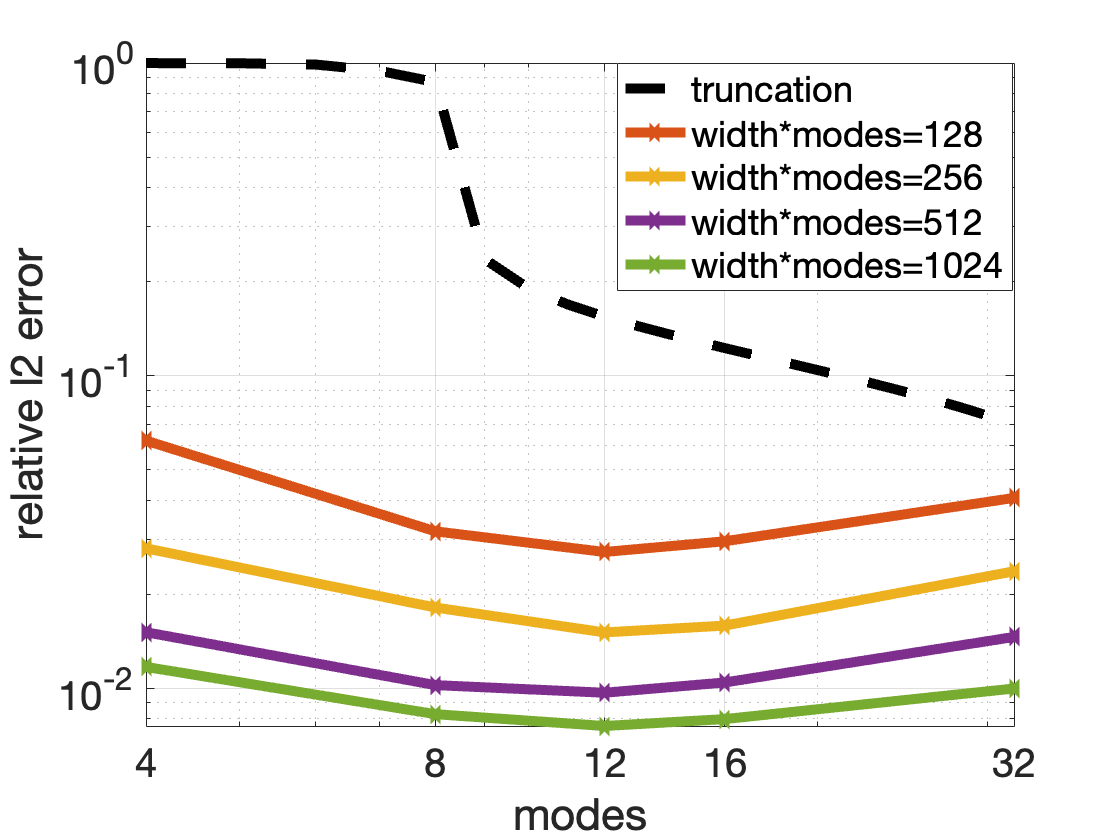
(a) Helmholtz Equation

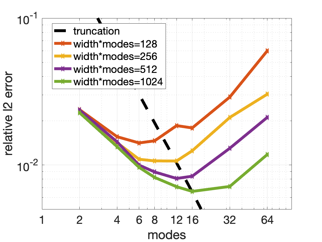
(b) Darcy Equation (discontinuous)

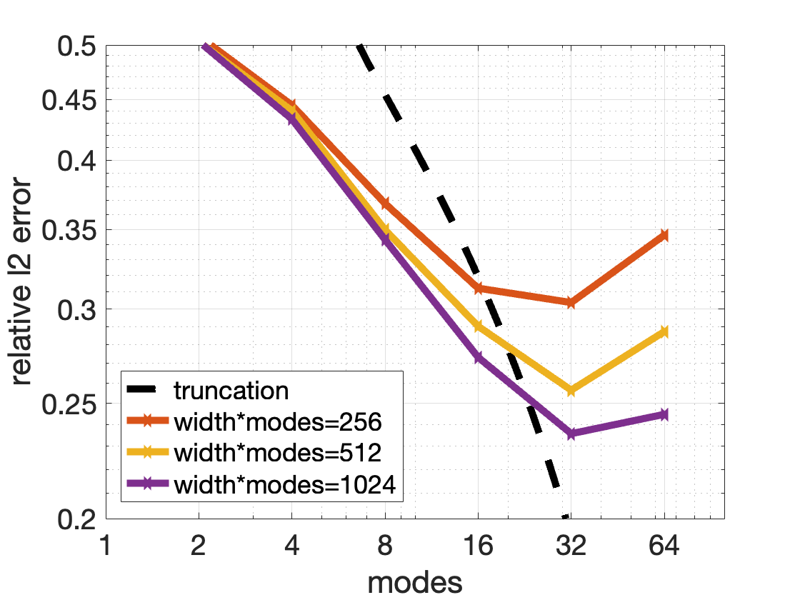
(c) Kolmogorov Flow

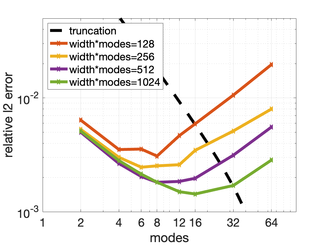
(d) Darcy Equation (smooth)

Figure 1: FNO model with different combinations of channel dimension (width) $d_{c}$ and Fourier modes $K$. In each curve, the models share roughly the same amount of model parameters because $d_{c}K$ is fixed at $C$, with $C$ changing between each curve. As $C$ increases, the overall error drops. The curves at any given fixed $C$ exhibit a “U”-shape, where the valley determines the optimal choice of modes $K$. The black dotted line is the error given by simply truncating the truth at the given number $K$ of Fourier modes; it is notable that the FNO is able to considerably improve on the Fourier truncation, suggesting the nonlinear approximation theoretic mechanisms at play in the architecture.

There are two types of numerical experiments that are suggested by the analysis in this paper: (i) to deploy the NNO for problems in non-periodic geometries, and in particular to explore choices of problem-adapted functions $\phi_{\ell,m},\psi_{\ell,m}$ in (1.2), aiming to develop intuition as to when it is an effective operator approximator; (ii) to determine the optimal distribution of parameters to obtain a given approximation error at least cost. We defer experiments of type (i) for future work and concentrate here on experiments of type (ii).

In the experiment sof type (ii) we fix a measure of the total number of parameters: the channel width (number of channels) multiplied by the number of Fourier basis functions. We identify the optimal choice of number of basis functions, in terms of the achieved test accuracy, for fixed total number of parameters. We conduct experiments on three sets of partial differential equations to study the balance between number of channels and number of Fourier modes: the Helmholtz Equation for wave-propagation in a heterogeneous medium, the Darcy Equation for porous medium flow, for both smooth and piecewise constant coefficients, and the forced two-dimensional Navier-Stokes equation, more specifically a Kolmogorov Flow.

For all three test cases, we use a 4-layer FNO model with the GeLU activation function, as in Li et al. (2021a), and a cosine annealing optimizer Loshchilov and Hutter (2016). In the Helmholtz and Darcy equations, we normalize the input and output functions by subtracting the pointwise mean and dividing by the pointwise standard deviation, with mean and pointwise variance computed from the training dataset; however in the Kolmogorov Flow, we do not use normalization. The results show that, in the range of parameter scenarios we consider, the Helmholtz Equation and Kolmogorov Flow are optimized by fixing the number of basis functions; in contrast the Darcy problem is optimized by increasing the total number of basis functions, given a fixed budget of total number of parameters. These results resonate with the different proofs of universal approximation for the FNO, the original one using an increasing number of Fourier modes to achieve smaller error Kovachki et al. (2021b) and the proof in this paper using only a single Fourier mode found via integration against the constant function; more generally the results suggest the need for deeper analysis of the deployment of parameters in neural operators to obtain the optimal error/cost tradeoff.

4.1 Helmholtz Equation

We consider the Helmholtz Equation as defined in De Hoop et al. (2022): the frequency is fixed at $10^{3}$ and the domain $[0,1]^{2}$ is used. A Neumann boundary condition is applied on the top of the domain, in the form of a hat function, and homogeneous Dirichlet boundary conditions are applied on the other three sides. The target operator maps the wave speed field to the disturbance field $\Phi^{\dagger}:c\mapsto u$. The probability measure on the inputs is a pointwise nonlinear transformation of a Gaussian random field: $c(x)=20+{\rm tanh}(\widetilde{c}(x)),\widetilde{c}\sim\mathcal{N}(0,(-\Delta+9)^{-2})$ where the Laplace operator is equipped with homogeneous Neumann boundary conditions.

4.2 Darcy Equation

The Darcy equation is widely studied in the operator learning literature and we use the set-up employed in Bhattacharya et al. (2021); Anandkumar et al. (2020). The target operator maps the coefficient field (permeability) to the solution field (pressure) $\Phi^{\dagger}:a\mapsto u$. We use $10^{3}$ data pairs to train the FNO model, each with resolution $141\times 141$.

We study two cases of the Darcy equation, differing in our choice of random input fields: piecewise-constant coefficients and log-normal coefficients. For the piecewise-constant case, the coefficient functions $a$ are samples from Gaussian random field $\widetilde{a}\sim\mathcal{N}(0,(-\Delta+9)^{-2})$ again with homogeneous Neumann boundary conditions. We apply a pointwise nonlinearity which assigns value $4$ or $12$ depending on the sign of the input: $a(x)=4$ if $\widetilde{a}(x)\leq 0$, $a(x)=12$ if $\widetilde{a}(x)>0$. For the log-normal case, the coefficient function $a$ is sampled from a lognormal distribution, which is equivalent to the exponential of the same Gaussian random field: $a(x)=\exp(\widetilde{a}(x))$.

4.3 Kolmogorov Flow

Our final example is the Kolmogorov Flow with set-up as defined in Li et al. (2021c). For this problem, we solve the periodic Navier-Stokes equation on a unit torus in two dimensions, with Reynolds number $5\times 10^{3}$; this Reynolds number leads to a challenging example in which more high-frequency structures are present in comparison to the previous cases considered in the literature. The equations may be formulated using the vorticity-stream function variables and the target operator we seek to learn maps the initial vorticity field to the vorticity field one time unit later: $\Phi^{\dagger}:u(t)\mapsto u(t+1)$. The dataset of input-output pairs computed from of 100 trajectories, with 80 used for training and 20 for testing. Each trajectory consists of 500 time units; the burn-in phase, during which chaotic dynamics forms, is removed from the trajectory. We sample the initial conditions from a Gaussian random field of similar form to the two preceding examples, but with $-\Delta$ subjected to periodic boundary conditions. In total, we use $4\times 10^{4}$ data pairs to train the FNO model, each with resolution $128\times 128$.

4.4 Results

We study the accuracy of the trained FNO for different combinations of channel dimension (or width) $d_{c}$ and Fourier modes $K$, with a given budget of the total number of parameters. Since the number of parameters scales as $O(d_{c}^{2}K^{2})$ for these 2-dimensional problems, we fix $d_{c}K=C$ as a convenient proxy to control the sizes of our models. The main theoretical result in this paper demonstrates that, in principle, universality can be achieved by simply retaining a single Fourier mode. In practice, it may be beneficial to include a larger number of modes, and we are interested in the optimal choice of $K$ (and hence $d_{c}$), given a fixed model size $C$. To study this refined question empirically, we consider different model sizes, with $C=128,256,512,...$, and scan over increments of the Fourier mode cut-off $K=2,4,8,...$. The results of this empirical study are collected in Figure 1, for the four settings summarized above; in each case, the relative $L^{2}$-errors are plotted as a function of the number of the Fourier truncation parameter $K$, and each solid curve represents the result of computations with a fixed number $C$ of model parameters. As a baseline, the dashed black line shows the average relative $L^{2}$-error that is achieved by a direct Fourier truncation of the reference output functions, as a function of $K$.

Overall, we observe that models with more parameters perform better. Moreover, for a fixed model size $C$, the solid curves describe a “U” shape as a function of $K$, implying that an optimal choice of the Fourier cut-off $K$ and channel dimension $d_{c}$ exists, at each given model size $C$. For the Helmholtz equation and for the Kolmogorov Flow, the optimal choice of Fourier cut-off $K$ is fixed across different model sizes, within the resolution of our experiments. The trained FNO for the Helmholtz Equation performs best with $K=12$. For the Kolmogorov Flow, the optimal choice is $K=32$ for all considered models. A priori, our theoretical results are not informative about the optimal distribution of parameters. However, they show that even a fixed choice of Fourier modes $K$, independent of the model size, is not in contradiction with the observed convergence to the underlying operator. This empirical observation would have been difficult to reconcile with previous universal approximation results, which require $K$ to grow without bound.

For the Darcy Equation, the optimal choice of modes clearly shifts to the right with increasing model size. When $C=d_{c}K=128$, the optimal choice of modes is $K=6$. When $d_{c}K=1024$, the optimal choice of modes is $K=16$. Thus, in this case, it appears to be optimal to invest additional degrees of freedom in a combination of increasing both $K$ and $d_{c}$. An interesting empirical observation in Figure 1 is that the trained FNO often beats the corresponding Fourier truncation of the true solution with the same number of modes. This is particularly apparent for the Darcy Equation, where even the FNO with a cut-off of only $K=2$ is able to achieve very accurate results, going considerably beyond the accuracy of the corresponding Fourier truncation baseline. This strongly indicates that the trained FNO discovers a non-linear mechanism to generate a well-calibrated set of higher-order Fourier modes, beyond $K=2$. Thus, non-linear composition combined with non-locality of the lowest Fourier modes enables accurate results even with very small $K$; this is the basic mechanism which underlies our main universality result. The empirical findings thus indicate the practical relevance of the basic mechanism identified in the present work, with implications beyond universal approximation.

(a) Helmholtz Equation

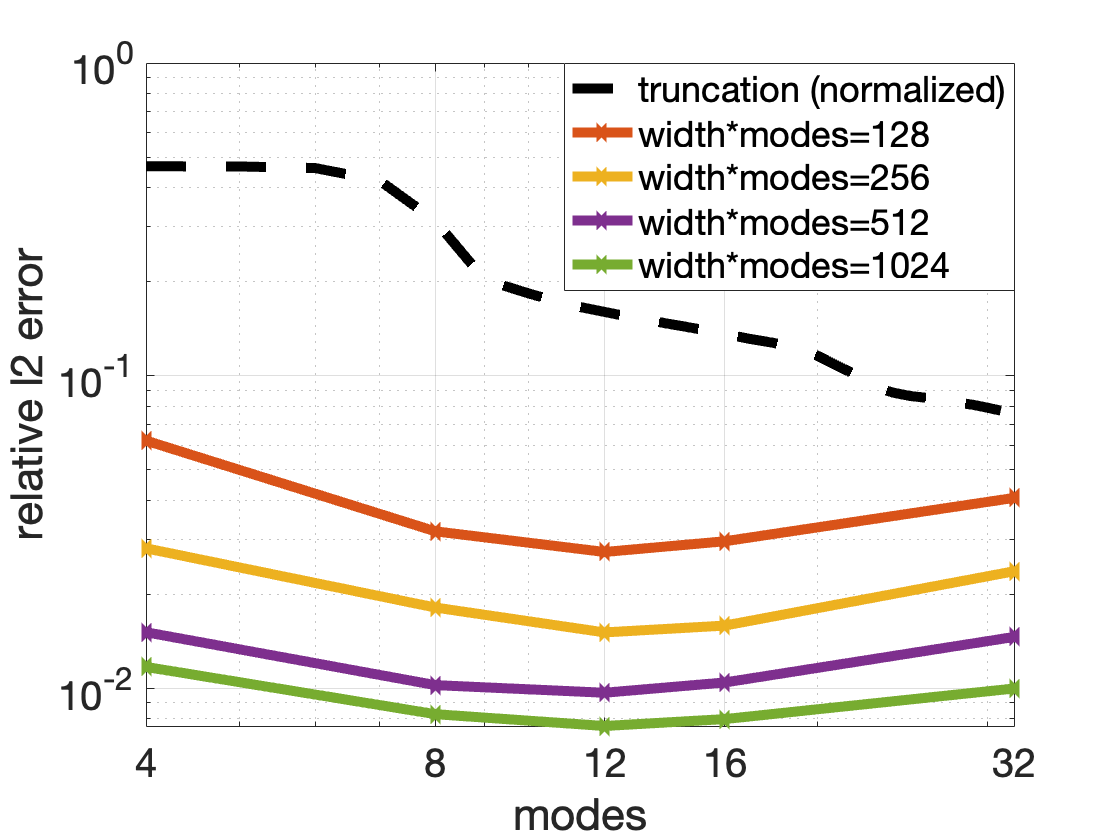
(b) Helmholtz Equation (normalized)

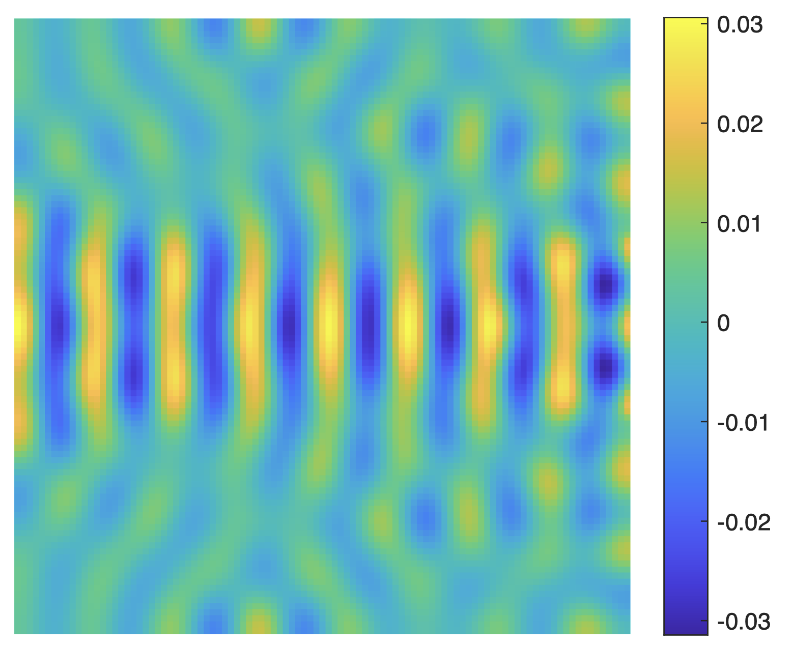
(c) Mean of Helmholtz

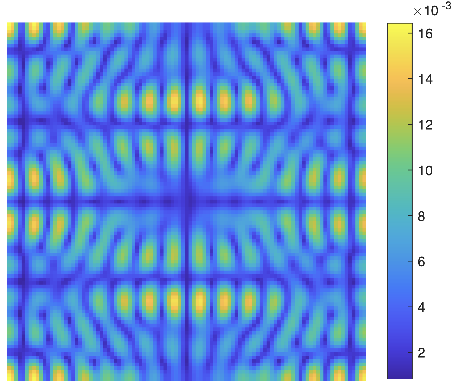
(d) Standard deviation of Helmholtz

Figure 2: The effect of normalization demonstrated for the Helmholtz Equation example. (a) Error rates as shown in Figure 1a). (b) Same as Figure 1a) but with error rates of the Fourier truncation including the effect of normalization. (c) and (d) show the mean and standard deviation, respectively, as used in the normalization process. Normalization assists in capturing lower modes but it does not affect the higher modes.

We include one final set of experiments designed to check that the effect of normalization (applied on the Helmholtz and both Darcy examples) is not responsible for effects apparent in Figure 1. Indeed we show that the desirable approximation effects we observe there cannot simply be attributed to the pre- and post-processing of the inputs and outputs of the neural network to ensure (empirical) mean zero and pointwise standard deviation one. To verify this assertion we show, in Figure 2, the error found simply by Fourier truncation, with and without the normalization applied. In Figure 2 (a), the truncation is done without the normalization. In Figure 2 (b), the truncation is done with the normalization: the solution function is first normalized by the pointwise mean and standard deviation, then truncated to the requisite number of Fourier modes, and finally denormalized, mimicking the procedure used in the model training. The truncation with normalization has a smaller error rate on the lower frequency modes, but the error at higher wavenumbers is similar to that arising without the truncation. The pointwise mean and standard deviation are shown in 2 (c, d), which demonstrates that the normalization captures some lower frequency structures. This experiment shows that normalization help to express the lower frequency components, but it does not account for the desirable approximation properties observed for the neural operator in Figure 1. The Figure 2 is for the Helmholtz equation, but similar effects are observed for the Darcy flow.

5 Discussion

This paper introduces a wide class of neural operators, the nonlocal neural operators (NNO). This class includes known frameworks such as the Fourier neural operator (FNO) as a special case, but, in contrast to FNO, applies to mappings between functions defined on general domains with arbitrary geometries. NNOs generalize FNOs by allowing for an expansion with respect to an arbitrary basis, not restricted to trigonometric functions. As shown in this work, the NNO is closely connected to a number of other recently proposed neural operator architectures. Reducing the NNO to its simplest possible form, we arrive at the averaging neural operator (ANO) as a special case. This ANO is based on only two minimal ingredients, both of which are indispensable for operator learning: non-linearity, by composition with ordinary neural networks, and non-locality, by averaging. Despite the simplicity of the resulting architecture, we show that the averaging neural operator (ANO) possesses a universal approximation property for a large class of operators, cf. Theorems 2.1 and 2.2.

This result implies not only universality of NNOs, leading to Theorems 1.1 and 1.2, but it also allows us to unify much of the theoretical analysis of an emerging zoo of neural operator architectures, including e.g. the general NO, FNO, low-rank NO, wavelet NO and Laplace-NO. As a consequence, we employ the ANO as an analysis tool to derive new universality results for all of these architectures, leading to Corollaries 3.1–3.5. These corollaries improve on known universal approximation results for general NOs and FNOs, and provide a first rigorous theoretical underpinning for the methodology in the case of low-rank, wavelet and Laplace NOs. We expect that our general universality result for the NNO, and its atomic core the ANO, will serve as a useful reference to prove universality for many other emerging neural operator architectures. In this context, we also point out close links of the ANO introduced in the present work with other recent proposed neural operator architectures, including the DeepONet and NOMAD architectures.

At a more fundamental level, the present work aims to shed new light on the role of nonlocality in operator learning for a general class of neural operators. Our main result is a universal approximation theorem, which shows that even very simple nonlocality in the form of an averaging operation is sufficient for the universality of neural operator architectures. As a consequence, we show that neural operator architectures possess a universal approximation property even if the nonlocality in the hidden layers is not capable of exploring the space of all integral operators, thus providing considerable scope for the introduction of nonlocality in new ways which may not rely on expansions in complete (e.g. Fourier or wavelet) bases. As a byproduct, we also further deepen our understanding of the Fourier neural operator; in particular, the present work strongly indicates that the importance of the Fourier transform for FNOs may be mainly in providing nonlocality to the architecture, with the particular choice of a Fourier basis playing only a subordinate role.

The present work provides substantial motivation to further study the optimal combination of nonlinearity and nonlocality in operator learning. First empirical results in this direction are presented in Section 4, focusing on the Fourier neural operator. Here, the relevant parameters are the channel dimension and the number of Fourier modes, corresponding to different distributions of nonlinearity and nonlocality in the architecture. Our empirical results show that the optimal distribution of parameters is likely problem dependent, but strongly indicate that the basic mechanism underlying our proof of universality is also relevant in practice; further numerical results, in tandem with extended analysis, will be necessary to gain deeper insight into the optimal trade-off, in terms of cost versus accuracy, between non-linearity and non-locality.

The fact that universality can be obtained even with a simple average as the only nonlocal ingredient in the hidden layers opens the way for the exploration of alternative neural operator architectures with guaranteed universality, relying on different choices of how nonlocality is introduced. The results of this work are also particularly relevant for future extensions of neural operator architectures to problems with non-periodic geometries and mappings between functions on different domains. We plan to expand on this topic, and the potential benefits of specific choices, in the future.

Acknowledgements The work of SL is supported by Postdoc.Mobility grant P500PT-206737 from the Swiss National Science Foundation. ZL is supported in part by the PIMCO Fellowship and Amazon AI4Science Fellowship. AMS is grateful for support through a Department of Defense Vannevar Bush Faculty Fellowship and from the Air Force Office of Scientific Research under MURI award number FA9550-20-1-0358 (Machine Learning and Physics-Based Modeling and Simulation).

Appendix A Detailed Proof Of Universal Approximation For ANO

A.1 Analysis Ingredients: Extension And Mollification

Lipschitz domains

We recall that a subset $\Omega\subset\mathbb{R}^{d}$ is a bounded Lipschitz domain, if $\Omega$ is open, the closure $\overline{\Omega}$ is compact, and the boundary $\partial\Omega=\overline{\Omega}\setminus\Omega$ is at least “Lipschitz regular”, in the sense that it can locally be thought of as the graph of a Lipschitz map. We refer to [Ern and Guermond, 2016, Section 2.1] for a rigorous mathematical definition. Lipschitz domains cover most domains encountered in physical applications. In particular, any bounded domain with piecewise smooth boundary is a Lipschitz domain.

Function extension for Lipschitz domains

In our proofs, it will sometimes be convenient to extend a given function $u:\Omega\to\mathbb{R}$, defined on a domain $\Omega\subset\mathbb{R}^{d}$, to a function $u:\mathbb{R}^{d}\to\mathbb{R}$, defined on all of $\mathbb{R}^{d}$. The following lemma shows that this is possible, while preserving smoothness of $u$, and relies on a classical result of Stein [Stein, 1970, Chapter 6, Theorem 5]:

[Periodic extension operator, see e.g. [Kovachki et al., 2021b, Lemma 41]] Let $\Omega\subset\mathbb{R}^{d}$ be a bounded Lipschitz domain. There exists a continuous, linear operator $\mathcal{E}:W^{s,p}(\Omega)\to W^{s,p}_{\mathrm{per}}(B)$ for any $s\geq 0$ and $p\in[1,\infty]$, where $B\subset\mathbb{R}^{d}$ is a bounded hypercube containing $\Omega\subset B$, such that for any $u\in W^{s,p}(\Omega)$:

1. $\mathcal{E}(u)|_{\Omega}=u$;

2. $\mathcal{E}(u)\in W^{s,p}_{\mathrm{per}}(B)$ is periodic on $B$ (including its derivatives).

Furthermore, $\mathcal{E}$ maps continuously differentiable functions to continuously differentiable functions, i.e. $\mathcal{E}(C^{s}(\overline{\Omega}))\subset C^{s}_{\mathrm{per}}(B)$ and hence defines a continuous mapping $\mathcal{E}:C^{s}(\overline{\Omega})\to C^{s}_{\mathrm{per}}(B)$.

Mollification (smoothing) of functions on Lipschitz domains

Recall that there exists a smooth mapping (a mollifier) $\rho:\mathbb{R}^{d}\to\mathbb{R}$, with properties $\rho(x)\in[0,1]$ for all $x\in\mathbb{R}^{d}$, $\rho(0)=1$, and $\rho(x)=0$ for $|x|\geq 1$. Furthermore we can normalize $\rho$ to enforce $\int_{\mathbb{R}^{d}}\rho(y)\,dy=1$. Any such $\rho$ defines a family of functions $\rho_{\delta}(x):=\delta^{-d}\rho(x/\delta)$, supported in a $\delta$-ball around the origin. Fixing such a family, we recall that the $\epsilon$-mollification of a function $u:\mathbb{R}^{d}\to\mathbb{R}$, $u\in L^{1}(\mathbb{R}^{d})$ is defined by a convolution $u_{\delta}(x):=(u\ast\rho_{\delta})(x)$, i.e.

$$u_{\delta}(x)=\int_{\mathbb{R}^{d}}u(x-y)\rho_{\delta}(y)\,dy.$$

It is well-known that $u_{\delta}$ is a smooth function for $\delta>0$, and that $u_{\delta}\to u$ in spaces such as arbitrary Sobolev spaces $W^{s,p}(\mathbb{R}^{d})$, or spaces of continuously differentiable functions $C^{s}(\mathbb{R}^{d})$, with respect to the respective norms. Mollification as defined above is a useful tool in analysis, but is not well-adapted to bounded domains. The papers Blouza and Le Dret [2001], Ern and Guermond [2016] develop a useful variant of mollification for bounded Lipschitz domains $\Omega\subset\mathbb{R}^{d}$, where additional care is needed to deal with the behavior near the boundary.

The following results follow from the proof of [Blouza and Le Dret, 2001, Theorem 2.4], or can alternatively be obtained from the construction and arguments in Ern and Guermond [2016]: [Adapted mollification in a Lipschitz domain] Let $\Omega\subset\mathbb{R}^{d}$ be a bounded Lipschitz domain. There exists a one-parameter family $\mathcal{M}_{\delta}$ of “mollification” operators, defining a linear mapping $\mathcal{M}_{\delta}:L^{1}(\Omega;\mathbb{R}^{k})\to C^{\infty}(\overline{\Omega};\mathbb{R}^{k})$, such that:

1. For any fixed $\delta>0$, integer $s,r\geq 0$, the mapping,

   $$\mathcal{M}_{\delta}:C^{s}(\overline{\Omega};\mathbb{R}^{k})\to C^{r}(\overline{\Omega};\mathbb{R}^{k}),$$

   is continuous. Furthermore, if $r\leq s$, then the operator norm is uniformly bounded, that is

   $$\sup_{\delta>0}\|\mathcal{M}_{\delta}\|_{C^{s}\to C^{r}}<\infty.$$

2. If $s\geq 0$ and $\mathsf{K}\subset C^{s}(\overline{\Omega};\mathbb{R}^{k})$ is a compact subset, then

   $$\lim_{\delta\to 0}\sup_{u\in\mathsf{K}}\|u-\mathcal{M}_{\delta}u\|_{C^{s}}=0.$$

   If $\delta\to\delta_{0}>0$, then $\mathcal{M}_{\delta}u\to\mathcal{M}_{\delta_{0}}u$ in $C^{s}$, uniformly for all $u\in K$.

3. For fixed $\delta>0$, integer $s,r\geq 0$, and $p\in[1,\infty)$, the mapping

   $$\mathcal{M}_{\delta}:W^{s,p}(\Omega;\mathbb{R}^{k})\to W^{r,p}(\Omega;\mathbb{R}^{k})$$

   is continuous.

4. If $s\geq 0$, $p\in[1,\infty)$ and $\mathsf{K}\subset W^{s,p}({\Omega};\mathbb{R}^{k})$ is a compact subset, then

   $$\lim_{\delta\to 0}\sup_{u\in\mathsf{K}}\|u-\mathcal{M}_{\delta}u\|_{W^{s,p}}=0.$$

   If $\delta\to\delta_{0}>0$, then $\mathcal{M}_{\delta}u\to\mathcal{M}_{\delta_{0}}u$ in $W^{s,p}$, uniformly for all $u\in K$.

At first sight, one might think that the result of Lemma A.1 could easily be obtained by extending the input function $u:\Omega\to\mathbb{R}^{k}$, to a function $u:\mathbb{R}^{d}\to\mathbb{R}^{k}$ by setting $u(x)=0$ for $\mathbb{R}^{d}\setminus\Omega$, and then use standard mollification on this extension to obtain a smooth approximant $u_{\delta}:\Omega\to\mathbb{R}^{k}$. While this approach ensures smoothness of the mollified function $u_{\delta}$, it does not ensure convergence in spaces defined with respect to the supremum norm, i.e. for $u\in C^{s}$ we generally have $\|u_{\delta}-u\|_{C^{s}}\not\to 0$ as $\delta\to 0$. The main technical issue is that extension by zero produces a jump discontinuity at the boundary; hence special care needs to be taken near the boundary [Blouza and Le Dret, 2001, Ern and Guermond, 2016].

The proof is based on the boundary-adapted construction of mollification in [Ern and Guermond, 2016, eq. (3.4a)], and only requires arguments in real analysis. We will not provide a detailed proof here.

In addition to Lemma A.1, we will furthermore need the following technical lemma: Fix $s\geq 0$. Let $\mathsf{K}\subset C^{s}(\overline{\Omega};\mathbb{R}^{k})$ be compact. Then for any $\delta>0$, the set

$$\mathsf{K}_{\delta}:=\mathsf{K}\cup\bigcup_{0<\delta^{\prime}\leq\delta}{\left\{\mathcal{M}_{\delta^{\prime}}u\,\middle|\,u\in\mathsf{K}\right\}},$$ (A.1)

is also compact in $C^{s}(\overline{\Omega};\mathbb{R}^{k})$.

Proof.

Let $v_{1},v_{2},\dots$ be an arbitrary sequence in $\mathsf{K}_{\delta}$. It suffices to prove that $v_{j}$ possesses a convergent subsequence $v_{j_{\ell}}\to v\in\mathsf{K}_{\delta}$. By definition of $\mathsf{K}_{\delta}$, there exists a sequence $u_{1},u_{2},\dots\in\mathsf{K}$, and $\delta_{1},\delta_{2},\dots\in(0,\delta]$, such that $v_{j}=\mathcal{M}_{\delta_{j}}u_{j}$ for all $j\in\mathbb{N}$. Since $\mathsf{K}$ is compact, there exists a convergent subsequence $u_{j_{\ell}}\to u\in\mathsf{K}$. Furthermore, extracting another subsequence if necessary (not reindexed), we may assume that $\delta_{j_{\ell}}\to\delta_{\infty}\in[0,\delta]$ converges to a limit. If $\delta_{\infty}>0$, let $v:=\mathcal{M}_{\delta_{\infty}}u$. If $\delta_{\infty}=0$, we set $v:=\mathcal{M}_{\delta_{\infty}}u=u$. We note that in either case, we have $v\in\mathsf{K}_{\delta}$. We claim that $v_{j_{\ell}}\to v$. To see this, note that

$$\limsup_{\ell\to\infty}\|v_{j_{\ell}}-v\|_{C^{s}} =\limsup_{\ell\to\infty}\|\mathcal{M}_{\delta_{j_{\ell}}}u_{j_{\ell}}-\mathcal{M}_{\delta_{\infty}}u\|_{C^{s}}$$

$$\leq\limsup_{\ell\to\infty}\|\mathcal{M}_{\delta_{j_{\ell}}}u_{j_{\ell}}-\mathcal{M}_{\delta_{j_{\ell}}}u\|_{C^{s}}$$

$$\qquad+\limsup_{\ell\to\infty}\|\mathcal{M}_{\delta_{j_{\ell}}}u-\mathcal{M}_{\delta_{\infty}}u\|_{C^{s}}$$

$$\leq\limsup_{\ell\to\infty}\|\mathcal{M}_{\delta_{j_{\ell}}}\|_{C^{s}\to C^{s}}\|u_{j_{\ell}}-u\|_{C^{s}}$$

$$\qquad+\limsup_{\ell\to\infty}\|\mathcal{M}_{\delta_{j_{\ell}}}u-\mathcal{M}_{\delta_{\infty}}u\|_{C^{s}}.$$

For fixed $u\in C^{s}$, we have $\mathcal{M}_{\delta_{j_{\ell}}}u\to\mathcal{M}_{\delta_{\infty}}u$ in $C^{s}$, and hence the second term converges to zero. Furthermore, by Lemma A.1 (1), the one-parameter family $\mathcal{M}_{\delta^{\prime}}:C^{s}\to C^{s}$ consists of uniformly bounded operators, such that

$$\sup_{\ell\in\mathbb{N}}\|\mathcal{M}_{\delta_{j_{\ell}}}\|_{C^{s}\to C^{s}}\leq\sup_{0<\delta^{\prime}\leq\delta}\|\mathcal{M}_{\delta^{\prime}}\|_{C^{s}\to C^{s}}<\infty.$$

From the convergence $u_{j_{\ell}}\to u$ in $C^{s}$, it thus follows that the first term above converges to zero. Thus, $v_{j_{\ell}}\to v$ as claimed. This shows that $\mathsf{K}_{\delta}$ is sequentially compact. ∎

A.2 Universal Approximation Of Neural Networks

It is well-known [Pinkus, 1999, Thm. 4.1] that a neural network architecture is universal in the class of $C^{s}$-functions between Euclidean vector spaces, provided that the activation function $\sigma$ is nonpolynomial and sufficiently smooth, $\sigma\in C^{s}$. This in turn implies universality of neural networks in Sobolev spaces $W^{s,p}$ of functions between Euclidean vector spaces. For the convenience of the reader, we include the relevant implication for the present work. Recall that, throughout the paper, we assume that the activation function $\sigma$ is $C^{\infty}$, nonpolynomial and Lipschitz continuous.

Let $\Omega\subset\mathbb{R}^{d}$ be a bounded Lipschitz domain. Then for any function $u:\Omega\to\mathbb{R}^{k}$, where $u$ belongs to either the space of continuously differentiable functions $C^{s}(\overline{\Omega};\mathbb{R}^{k})$, or the Sobolev space $W^{s,p}(\Omega;\mathbb{R}^{k})$, for integer $s\geq 0$ and $p\in[1,\infty)$, and for any $\epsilon>0$, there exists a neural network $\widetilde{u}:\Omega\to\mathbb{R}^{k}$ with activation function $\sigma$, such that

$$\sup_{x\in\Omega}|u(x)-\widetilde{u}(x)|\leq\epsilon.$$

Proof.

Step 1: We first assume that $u\in C^{s}(\overline{\Omega};\mathbb{R}^{k})$. By Lemma A.1, there exists a (periodic) extension $U:\mathbb{R}^{d}\to\mathbb{R}$, such that $u(x)=U(x)$ for $x\in\Omega$, and $U\in C^{s}(\mathbb{R}^{d};\mathbb{R}^{k})$. It follows from [Pinkus, 1999, Thm. 4.1] that for any $\epsilon>0$, there exists a neural network $\widetilde{u}:\mathbb{R}^{d}\to\mathbb{R}$, such that

$$\|u-\widetilde{u}\|_{C^{s}(\overline{\Omega};\mathbb{R}^{k})}=\sup_{|\alpha|\leq s}\sup_{x\in\overline{\Omega}}|D^{\alpha}U(x)-D^{\alpha}\widetilde{u}(x)|\leq\epsilon.$$

Step 2: If $u\in W^{s,p}(\Omega;\mathbb{R}^{k})$, then we note that by Lemma A.1, the boundary-adapted mollification $u_{\delta}:=\mathcal{M}_{\delta}u$ converges to $u$ as $\delta\to 0$. Let $\epsilon>0$ be given. Choose $\delta>0$ sufficiently small, such that

$$\|u-u_{\delta}\|_{W^{s,p}(\Omega;\mathbb{R}^{k})}\leq\epsilon/2.$$

We note that $C^{s+1}(\overline{\Omega};\mathbb{R}^{k}){\hookrightarrow}W^{s,p}(\Omega;\mathbb{R}^{k})$ has a continuous embedding, and hence there exists a constant $C_{0}>0$, such that

$$\|{\,\cdot\,}\|_{W^{s,p}(\Omega;\mathbb{R}^{k})}\leq C_{0}\|{\,\cdot\,}\|_{C^{s+1}(\overline{\Omega};\mathbb{R}^{k})}.$$

Now note that there exists a neural network $\widetilde{u}$, such that $\|u_{\delta}-\widetilde{u}\|_{C^{s+1}(\overline{\Omega};\mathbb{R}^{k})}\leq\epsilon/2C_{0}$; this follows since $u_{\delta}\in C^{s+1}(\overline{\Omega};\mathbb{R}^{k})$, by Step 1. Combining these estimates, we obtain

$$\|u-\widetilde{u}\|_{W^{s,p}(\Omega;\mathbb{R}^{k})} \leq\|u-u_{\delta}\|_{W^{s,p}(\Omega;\mathbb{R}^{k})}+\|u_{\delta}-\widetilde{u}\|_{W^{s,p}(\Omega;\mathbb{R}^{k})}$$

$$\leq\epsilon/2+C_{0}\|u_{\delta}-\widetilde{u}\|_{C^{s+1}(\overline{\Omega};\mathbb{R}^{k})}$$

$$\leq\epsilon.$$

This concludes our proof. ∎

A.3 A Dense Subset Of Operators

One crucial ingredient in the proof of universal approximation for averaging neural operators is the fact that it is possible to reduce the problem for a general operator $\Psi^{\dagger}:C^{s}(\overline{\Omega};\mathbb{R}^{k})\to C^{s^{\prime}}(\overline{\Omega};\mathbb{R}^{k^{\prime}})$ (or $\Psi^{\dagger}:W^{s,p}(\Omega;\mathbb{R}^{k})\to W^{s^{\prime},p^{\prime}}(\Omega;\mathbb{R}^{k^{\prime}})$, respectively), to one for a simpler class of operators which can be written in the form,

$$\widetilde{\Psi}^{\dagger}(u)=\sum_{j=1}^{J}\alpha_{j}(u)\eta_{j},$$ (A.2)

where $\eta_{1},\dots,\eta_{J}$ are functions in $C^{s^{\prime}}(\overline{\Omega};\mathbb{R}^{k^{\prime}})$ (resp. in $W^{s^{\prime},p^{\prime}}(\Omega;\mathbb{R}^{k^{\prime}})$), and $\alpha_{1},\dots,\alpha_{J}:L^{1}(\Omega;\mathbb{R}^{k})\to\mathbb{R}$ are continuous nonlinear functionals, defined on the space of integrable functions. This is the content of the following two propositions. The first version is formulated for operators between spaces of continuously differentiable functions and the second between Sobolev spaces.

Let $\Psi^{\dagger}:C^{s}(\overline{\Omega};\mathbb{R}^{k})\to C^{s^{\prime}}(\overline{\Omega};\mathbb{R}^{k^{\prime}})$ be a continuous operator. Let $\mathsf{K}\subset C^{s}(\overline{\Omega};\mathbb{R}^{k})$ be a compact subset. Then for any $\epsilon>0$, there exist $J\in\mathbb{N}$, functions $\eta_{1},\dots,\eta_{J}\in C^{s^{\prime}}(\overline{\Omega};\mathbb{R}^{k^{\prime}})$, and continuous functionals $\alpha_{1},\dots,\alpha_{J}:L^{1}(\Omega;\mathbb{R}^{k})\to\mathbb{R}$, such that the operator $\widetilde{\Psi}^{\dagger}:L^{1}(\Omega;\mathbb{R}^{k})\to C^{s^{\prime}}(\overline{\Omega};\mathbb{R}^{k^{\prime}})$, $\widetilde{\Psi}^{\dagger}(u):=\sum_{j=1}^{J}\alpha_{j}(u)\eta_{j}$, satisfies

$$\sup_{u\in\mathsf{K}}\left\|\Psi^{\dagger}(u)-\widetilde{\Psi}^{\dagger}(u)\right\|_{C^{s^{\prime}}}\leq\epsilon.$$

We emphasize that even though the underlying operator $\Psi^{\dagger}(u)$ is only defined for $u\in C^{s}(\overline{\Omega};\mathbb{R}^{k})$, and will generally not possess any continuous extension to an operator defined for $u\in L^{1}(\Omega;\mathbb{R}^{k})$, the above Proposition A.3 constructs a continuous operator $\widetilde{\Psi}^{\dagger}:L^{1}(\Omega;\mathbb{R}^{k})\to C^{s^{\prime}}(\overline{\Omega};\mathbb{R}^{k^{\prime}})$, whose restriction to compact $\mathsf{K}\subset C^{s}(\overline{\Omega};\mathbb{R}^{k})$ provides a good approximation, $\Psi^{\dagger}|_{\mathsf{K}}\approx\widetilde{\Psi}^{\dagger}|_{\mathsf{K}}$. In this context note that $L^{1}(\Omega;\mathbb{R}^{k})\supset C^{s}(\overline{\Omega};\mathbb{R}^{k})$.

Proof.

Let us first point out that we may without loss of generality assume $k^{\prime}=1$, in the following; indeed we can identify $C^{s^{\prime}}(\overline{\Omega};\mathbb{R}^{k})=[C^{s^{\prime}}(\overline{\Omega};\mathbb{R})]^{k}$, and thus it will suffice to approximate each component of the mapping $\Psi^{\dagger}:C^{s}(\overline{\Omega};\mathbb{R}^{k})\to[C^{s^{\prime}}(\overline{\Omega};\mathbb{R})]^{k}$, individually. The $j$-th component defines a mapping $\Psi^{\dagger}_{j}:C^{s}(\overline{\Omega};\mathbb{R}^{k})\to C^{s^{\prime}}(\overline{\Omega};\mathbb{R})$. Henceforth we use the notation $C^{s^{\prime}}(\overline{\Omega}):=C^{s^{\prime}}(\overline{\Omega};\mathbb{R}).$

Step 1: (construction of $\eta_{1},\dots,\eta_{J}$) Our first goal is to construct suitable $\eta_{1},\dots,\eta_{J}$. To this end, we consider $\mathsf{K}^{\prime}:=\Psi^{\dagger}(\mathsf{K})\subset C^{s^{\prime}}(\overline{\Omega})$. Note that since $\mathsf{K}$ is compact, and $\Psi^{\dagger}$ is continuous, its image $\mathsf{K}^{\prime}$ is also compact. Let $B\supset\Omega$ be a bounding box, containing $\overline{\Omega}$ in its interior. By Lemma A.1, there exists a continuous extension mapping

$$\mathcal{E}:C^{s^{\prime}}(\overline{\Omega})\to C^{s^{\prime}}_{\mathrm{per}}(B),$$

where $C^{s^{\prime}}_{\mathrm{per}}(B)$ denotes the space of continuously differentiable functions $w:B\to\mathbb{R}$ on the Cartesian domain $B$, possessing periodic derivatives up to order $s^{\prime}$. Since $\mathsf{K}^{\prime}\subset C^{s^{\prime}}(\overline{\Omega})$ is compact, it follows that also $\mathsf{K}^{\prime}_{\mathrm{per}}:=\mathcal{E}(\mathsf{K}^{\prime})$ is a compact subset of $C^{s^{\prime}}_{\mathrm{per}}(B)$. Given this periodicity, we can identify $B\simeq\mathbb{T}^{d}$ with the periodic torus in a canonical way. Let $\eta_{1},\eta_{2},\dots$ denote an enumeration of the $L^{2}$-orthogonal (real) Fourier sine/cosine basis in $L^{2}_{\mathrm{per}}(B)$. Fix $\delta>0$, and let $w_{\delta}:B\to\mathbb{R}$ be the standard mollification of the periodic function $w:B\to\mathbb{R}$. Since $\mathsf{K}^{\prime}_{\mathrm{per}}\subset C^{s^{\prime}}_{\mathrm{per}}(B)$ is compact, the set ${\left\{w_{\delta}\,\middle|\,w\in\mathsf{K}^{\prime}_{\mathrm{per}}\right\}}$ is uniformly bounded in the $C^{r^{\prime}}$-norm for any given $r^{\prime}>s^{\prime}$. In particular, it follows from classical results in harmonic analysis [Jackson, 1930, Chap. 1, Sect. 3], that approximation by Fourier series converges uniformly over ${\left\{w_{\delta}\,\middle|\,w\in\mathsf{K}^{\prime}_{\mathrm{per}}\right\}}$, i.e.

$$\lim_{N\to\infty}\sup_{w\in\mathsf{K}^{\prime}_{\mathrm{per}}}\left\|w_{\delta}-\textstyle\sum_{j=1}^{J}\langle w_{\delta},\eta_{j}\rangle_{L^{2}}\eta_{j}\right\|_{C^{s^{\prime}}_{\mathrm{per}}(B)}=0.$$

Furthermore, $\lim_{\delta\to 0}\|w_{\delta}-w\|_{C^{s^{\prime}}}=0$, uniformly over $\mathsf{K}^{\prime}_{\mathrm{per}}$. In particular, given $\epsilon>0$, we can first find $\delta=\delta(\epsilon)>0$, such that $\sup_{w\in\mathsf{K}^{\prime}_{\mathrm{per}}}\|w-w_{\delta}\|_{C^{s^{\prime}}}\leq\epsilon/2,$ and then $J\in\mathbb{N}$, such that $\sup_{w\in\mathsf{K}^{\prime}_{\mathrm{per}}}\left\|w_{\delta}-\textstyle\sum_{j=1}^{J}\langle w_{\delta},\eta_{j}\rangle_{L^{2}}\eta_{j}\right\|_{C^{s^{\prime}}_{\mathrm{per}}(B)}\leq\epsilon/2.$ It follows from the triangle inequality that

$$\sup_{w\in\mathsf{K}^{\prime}_{\mathrm{per}}}\left\|w-\textstyle\sum_{j=1}^{J}\langle w_{\delta},\eta_{j}\rangle_{L^{2}}\eta_{j}\right\|_{C^{s^{\prime}}_{\mathrm{per}}(B)}\leq\epsilon.$$

This defines our choice of $\eta_{1},\dots,\eta_{J}$. Note that we also have the identity

$$\sum_{j=1}^{J}\langle w_{\delta},\eta_{j}\rangle_{L^{2}}=\sum_{j=1}^{J}\langle w,\eta_{j,\delta}\rangle_{L^{2}}.$$

We now recall that $\Omega\subset B$, and $\mathcal{E}$ is an extension operator, so that $\mathcal{E}(v)|_{\Omega}=v$ for all $v\in\mathsf{K}^{\prime}$. Furthermore, we have $\mathsf{K}^{\prime}_{\mathrm{per}}=\mathcal{E}(\mathsf{K}^{\prime})$ and $\mathsf{K}^{\prime}=\Psi^{\dagger}(\mathsf{K})$, by definition. As a consequence, it follows that,

$$\sup_{u\in\mathsf{K}}\left\|\Psi^{\dagger}(u)-\textstyle\sum_{j=1}^{J}\langle\mathcal{E}(\Psi^{\dagger}(u)),\eta_{j,\delta}\rangle_{L^{2}}\eta_{j}\right\|_{C^{s^{\prime}}(\overline{\Omega})} =\sup_{v\in\mathsf{K}^{\prime}}\left\|v-\textstyle\sum_{j=1}^{J}\langle\mathcal{E}(v),\eta_{j,\delta}\rangle_{L^{2}}\eta_{j}\right\|_{C^{s^{\prime}}(\overline{\Omega})}$$

$$=\sup_{v\in\mathsf{K}^{\prime}}\left\|\mathcal{E}(v)-\textstyle\sum_{j=1}^{J}\langle\mathcal{E}(v),\eta_{j,\delta}\rangle_{L^{2}}\eta_{j}\right\|_{C^{s^{\prime}}(\overline{\Omega})}$$

$$\leq\sup_{v\in\mathsf{K}^{\prime}}\left\|\mathcal{E}(v)-\textstyle\sum_{j=1}^{J}\langle\mathcal{E}(v),\eta_{j,\delta}\rangle_{L^{2}}\eta_{j}\right\|_{C^{s^{\prime}}_{\mathrm{per}}(B)}$$

$$=\sup_{w\in\mathsf{K}^{\prime}_{\mathrm{per}}}\left\|w-\textstyle\sum_{j=1}^{J}\langle w,\eta_{j,\delta}\rangle_{L^{2}}\eta_{j}\right\|_{C^{s^{\prime}}_{\mathrm{per}}(B)}\leq\epsilon.$$

Step 2: (construction of $\alpha_{1},\dots,\alpha_{N}$)

Given the results of Step 1, let us define a nonlinear functional $\beta_{j}:C^{s}(\overline{\Omega};\mathbb{R}^{k})\to\mathbb{R}$ by $\beta_{j}(u):=\langle\mathcal{E}(\Psi^{\dagger}(u)),\eta_{j,\delta}\rangle_{L^{2}}$. Then, by Step 1, we have

$$\sup_{u\in\mathsf{K}}\left\|\Psi^{\dagger}(u)-\textstyle\sum_{j=1}^{J}\beta_{j}(u)\eta_{j}\right\|_{C^{s^{\prime}}}\leq\epsilon.$$ (A.3)

This is almost the claimed result, except that $\beta_{j}$ does not define a continuous functional $L^{1}(\Omega;\mathbb{R}^{k})\to\mathbb{R}$. To remedy this, we rely on mollification adapted to the bounded Lipschitz domain $\Omega$. Let $\delta>0$ denote a mollification parameter. By Lemma A.1, there exists a continuous operator $\mathcal{M}_{\delta}:L^{1}(\Omega;\mathbb{R}^{k})\to C^{s}(\overline{\Omega};\mathbb{R}^{k})$, such that over the compact set $\mathsf{K}\subset C^{s}(\overline{\Omega};\mathbb{R}^{k})$, we have

$$\sup_{u\in\mathsf{K}}\|u-\mathcal{M}_{\delta}u\|_{C^{s}}\to 0,$$

as $\delta\to 0$.

We intend to define $\alpha_{j}:L^{1}(\Omega;\mathbb{R}^{k})\to\mathbb{R}$ by $\alpha_{j}(u):=\beta_{j}(\mathcal{M}_{\delta}u)$ for suitably chosen $\delta>0$. Recall that for fixed $\delta_{0}>0$, the set $\mathsf{K}_{\delta}$ defined by

$$\mathsf{K}_{\delta}:=\bigcup_{0<\delta\leq\delta_{0}}\mathcal{M}_{\delta}(\mathsf{K}),$$

is a compact subset of $C^{s}(\overline{\Omega};\mathbb{R}^{k})$, by Lemma A.1. Note that for any $j=1,\dots,N$, we have a continuous mapping $\beta_{j}:\mathsf{K}_{\delta}\to\mathbb{R}$. Since $\mathsf{K}_{\delta}$ is compact, it follows that there exists a continuous modulus of continuity $\omega:[0,\infty)\to[0,\infty)$, satisfying $\omega(0)=0$, such that

$$|\beta_{j}(u)-\beta_{j}(u^{\prime})|\leq\omega(\|u-u^{\prime}\|_{C^{s}}),\quad\forall\,u,u^{\prime}\in\mathsf{K}_{\delta},$$

holds for all $j=1,\dots,N$. It follows that

$$|\beta_{j}(u)-\beta_{j}(\mathcal{M}_{\delta}u)|\leq\omega(\|u-\mathcal{M}_{\delta}u\|_{C^{s}}),$$

for any $0<\delta\leq\delta_{0}$. By Lemma A.1, $\mathcal{M}_{\delta}u\to u$ converges uniformly over $u\in\mathsf{K}$, so that we may conclude

$$\lim_{\delta\to 0}\sup_{u\in\mathsf{K}}|\beta_{j}(u)-\beta_{j}(\mathcal{M}_{\delta}u)|\leq\lim_{\delta\to 0}\omega\left(\textstyle\sup_{u\in\mathsf{K}}\|u-\mathcal{M}_{\delta}u\|_{C^{s}}\right)=0.$$

In particular, we can choose $\delta>0$ sufficiently small, to ensure that $\alpha_{j}(u):=\beta_{j}(\mathcal{M}_{\delta}u)$ satisfies

$$\sup_{u\in\mathsf{K}}|\beta_{j}(u)-\alpha_{j}(u)|\leq\frac{\epsilon}{J\max_{j=1,\dots,J}\|\eta_{j}\|_{C^{s^{\prime}}}},$$ (A.4)

for all $j=1,\dots,J$. Since $\delta>0$, we also note that $\mathcal{M}_{\delta}:L^{1}(\Omega;\mathbb{R}^{k})\to C^{s}(\overline{\Omega};\mathbb{R}^{k})$ is a continuous mapping, and hence $\alpha_{j}=\beta_{j}\circ\mathcal{M}_{\delta}$ is continuous as a mapping $\alpha_{j}:L^{1}(\Omega;\mathbb{R}^{k})\to\mathbb{R}$.

Step 3: (Conclusion) Combining (A.3) with (A.4), we obtain

$$\sup_{u\in\mathsf{K}}\left\|\Psi^{\dagger}(u)-\textstyle\sum_{j=1}^{J}\alpha_{j}(u)\eta_{j}\right\|_{C^{s^{\prime}}} \leq\sup_{u\in\mathsf{K}}\left\|\Psi^{\dagger}(u)-\textstyle\sum_{j=1}^{J}\beta_{j}(u)\eta_{j}\right\|_{C^{s^{\prime}}}$$

$$\qquad+\sup_{u\in\mathsf{K}}\left\|\textstyle\sum_{j=1}^{J}[\beta_{j}(u)-\alpha_{j}(u)]\eta_{j}\right\|_{C^{s^{\prime}}}$$

$$\leq\sup_{u\in\mathsf{K}}\left\|\Psi^{\dagger}(u)-\textstyle\sum_{j=1}^{J}\beta_{j}(u)\eta_{j}\right\|_{C^{s^{\prime}}}$$

$$\qquad+N\|\eta_{j}\|_{C^{s^{\prime}}}\max_{j=1,\dots,N}\sup_{u\in\mathsf{K}}|\beta_{j}(u)-\alpha_{j}(u)|$$

$$\leq 2\epsilon.$$

As $\epsilon>0$ was arbitrary, the claim of Proposition A.3 now follows. ∎

We can also formulate a similar result for operators between Sobolev spaces. As the proof is almost identical to the proof of Proposition A.3, and essentially follows by replacing $C^{s}$ by $W^{s,p}$ and analogously in the output space, we forego the details of this argument, and only state the final result.

Let $\Psi^{\dagger}:W^{s,p}(\Omega;\mathbb{R}^{k})\to W^{s^{\prime},p^{\prime}}(\Omega;\mathbb{R}^{k^{\prime}})$ be a continuous operator. Let $\mathsf{K}\subset W^{s,p}(\Omega;\mathbb{R}^{k})$ be a compact subset. Then for any $\epsilon>0$, there exist $\eta_{1},\dots,\eta_{J}\in W^{s^{\prime},p^{\prime}}(\Omega;\mathbb{R}^{k^{\prime}})$, and continuous functionals $\alpha_{1},\dots,\alpha_{N}:L^{1}(\Omega;\mathbb{R}^{k})\to\mathbb{R}$, such that

$$\sup_{u\in\mathsf{K}}\left\|\Psi^{\dagger}(u)-\textstyle\sum_{j=1}^{J}\alpha_{j}(u)\eta_{j}\right\|_{W^{s^{\prime},p^{\prime}}}\leq\epsilon.$$

A.4 Approximation Of Nonlinear Functionals By The Averaging Neural Operator

Given the result of Proposition A.3 and A.3 in the last section, a core ingredient in our proof of universal approximation for averaging neural operators will be the approximation of nonlinear functionals $\alpha:L^{1}(\Omega;\mathbb{R}^{k})\to\mathbb{R}$ by averaging neural operators. In the present section, we will show that any nonlinear a functional $\alpha:L^{1}(\Omega;\mathbb{R}^{k})\to\mathbb{R}$, $u\mapsto\alpha(u)$, can be approximated by an averaging neural operator in a suitable sense. This is the subject of the following lemma: Let $\alpha:L^{1}(\Omega;\mathbb{R}^{k})\to\mathbb{R}$ be a continuous nonlinear functional. Let $\mathsf{K}\subset L^{1}(\Omega;\mathbb{R}^{k})$ be a compact set, consisting of bounded functions, $\sup_{u\in\mathsf{K}}\|u\|_{L^{\infty}}<\infty$. Then for any $\epsilon>0$, there exists an averaging neural operator $\widetilde{\alpha}:L^{1}(\Omega;\mathbb{R}^{k})\to L^{1}(\Omega)$, all of whose output functions are constant so that we may also view $\widetilde{\alpha}$ as a function $\widetilde{\alpha}:L^{1}(\Omega;\mathbb{R}^{k})\to\mathbb{R}$, such that

$$\sup_{u\in\mathsf{K}}|\alpha(u)-\widetilde{\alpha}(u)|\leq\epsilon.$$

We note that the construction in our proof of Lemma A.4 (cp. (A.12) below) actually defines an averaging neural operator with (1) a lifting layer represented by $R(u(x),x)$, (2) a single hidden layer $v(x)\mapsto\sigma\left(\fint_{\Omega}v(y)\,dy\right)$, and (3) the projection layer $Q(v,x):=q_{1}(v)$, where $q_{1}$ is a neural network depending only on $v$. Hence, the result of Lemma A.4, and as a consequence the universal approximation property as described in Theorems 2.1 and 2.2, can be achieved with a single evaluation of the averaging operation: $L=1$.

Proof.

(Lemma A.4) Let $\alpha:L^{1}(\Omega;\mathbb{R}^{k})\to\mathbb{R}$ be a continuous functional. Let $\mathsf{K}\subset L^{1}(\Omega;\mathbb{R}^{k})$ be a compact set. Fix $\epsilon>0$. Our aim is to show that there exists an averaging neural operator $\widetilde{\alpha}:L^{1}(\Omega;\mathbb{R}^{k})\to L^{1}(\Omega)$ with constant output, such that

$$\sup_{u\in\mathsf{K}}|\alpha(u)-\widetilde{\alpha}(u)|\leq\epsilon.$$

To prove this, note that we can identify any $u\in L^{1}(\Omega;\mathbb{R}^{k})$ with a function in $L^{1}(B;\mathbb{R}^{k})$, via an extension of $u(x):=0$ for $x\in B\setminus\Omega$. Using this identification, the compact subset $\mathsf{K}\subset L^{1}(\Omega;\mathbb{R}^{k})$ can be identified with a compact subset of $L^{1}(\mathbb{R}^{d};\mathbb{R}^{k})$. Fix a smooth mollifier $\rho\in C^{\infty}$, and denote $\rho_{\delta}(x):=\delta^{-d}\rho(x/\delta)$ for $\delta>0$. We denote by $u_{\delta}(x)=(u\ast\rho_{\delta})(x)$ the mollification of $u$ (extended to all of $\mathbb{R}^{d}$ by $0$ outside of $\Omega$). Since $\mathsf{K}\subset L^{1}(\Omega;\mathbb{R}^{k})$ is compact, it follows that

$$\lim_{\delta\to 0}\sup_{u\in\mathsf{K}}\|u-u_{\delta}\|_{L^{1}(\Omega;\mathbb{R}^{k})}=0.$$

Since $\alpha:L^{1}(\Omega;\mathbb{R}^{k})\to\mathbb{R}$ is continuous, it follows that the mapping $\alpha_{\delta}:L^{1}(B,\mathbb{R}^{k})\to\mathbb{R}$ defined by $\alpha_{\delta}(u):=\alpha(u_{\delta})$, for $\delta>0$, converges uniformly over $\mathsf{K}$, as $\delta\to 0$:

$$\lim_{\delta\to 0}\sup_{u\in\mathsf{K}}|\alpha(u)-\alpha_{\delta}(u)|\leq\lim_{\delta\to 0}\sup_{u\in\mathsf{K}}|\alpha(u)-\alpha(u_{\delta})|=0.$$ (A.5)

The idea is now that, for any choice of orthonormal basis $\xi_{1},\xi_{2},\dots$ of $L^{2}(\Omega;\mathbb{R}^{k})$, which we may additionally choose to be smooth, $\xi_{j}\in C^{\infty}(\Omega;\mathbb{R}^{k})$, we have uniform convergence,

$$\sup_{u\in\mathsf{K}}\left\|u_{\delta}-\textstyle\sum_{j=1}^{J}\langle u_{\delta},\xi_{j}\rangle_{L^{2}}\xi_{j}\right\|_{L^{1}(B;\mathbb{R}^{k})}\to 0,$$ (A.6)

as $N\to\infty$. We note that the expression in (A.6) is well-defined, since $\mathsf{K}\subset L^{1}\cap L^{\infty}\subset L^{2}$, by assumption. Furthermore, $\mathsf{K}\subset L^{2}$ is compact in the $L^{2}$-norm; this entails the uniform convergence (A.6). With the convention that $u$ and $\xi_{j}$ are expanded by $0$ outside of $\Omega$, we have

$$\begin{aligned} \langle u_{\delta},\xi_{j}\rangle_{L^{2}}&=\int_{\Omega}u_{\delta}(y)\cdot\xi_{j}(y)\,dy=\int_{\mathbb{R}^{d}}(u\ast\rho_{\delta})(y)\cdot\xi_{j}(y)\,dy\\ &=\int_{\mathbb{R}^{d}}u(y)\cdot(\xi_{j}\ast\rho_{\delta})(y)\,dy=\fint_{\Omega}u(y)\cdot{\xi}_{j,\delta}(y)\,dy,\end{aligned}$$ (A.7)

where we have defined ${\xi}_{j,\delta}(y):=|\Omega|(\xi_{j}\ast\rho_{\delta})(y)$. Hence, if we define $\alpha_{\delta,J}:L^{1}(\Omega;\mathbb{R}^{k})\to\mathbb{R}$ by

$$\alpha_{\delta,J}(u):=\alpha\left(\sum_{j=1}^{J}\left(\fint_{\Omega}u(y)\cdot\xi_{j,\delta}(y)\,dy\right)\,\xi_{j}\right),$$

then it follows from (A.5), (A.6) and (A.7), that for $\delta=\delta(\mathsf{K})>0$ sufficiently small, and $J=J(\delta,\mathsf{K})\in\mathbb{N}$ sufficiently large, we have $\sup_{u\in\mathsf{K}}|\alpha_{\delta}(u)-\alpha_{\delta,J}(u)|\leq\epsilon/2$. To indicate the connection to averaging neural operators, we note that we can write $\alpha_{\delta,J}$ as the following composition:

$$u\mapsto\left(\fint_{\Omega}u(y)\cdot\xi_{1,\delta}(y)\,dy,\dots,\fint_{\Omega}u(y)\cdot\xi_{J,\delta}(y)\,dy\right)\mapsto\alpha\left(\sum_{j=1}^{J}\left(\fint_{\Omega}u(y)\cdot\xi_{j,\delta}(y)\,dy\right)\,\xi_{j}\right).$$

The first of these mapping requires computation of certain averages (albeit against a function $\xi_{j,\delta}$). Approximation of this mapping clearly requires nonlocality. The second mapping defines a continuous function $\beta:\mathbb{R}^{J}\to\mathbb{R}$, $c=(c_{1},\dots,c_{J})\mapsto\alpha\left(\sum_{j=1}^{J}c_{j}\xi_{j}\right)$. Approximation of this mapping is possible by ordinary neural networks; this requires nonlinearity, but does not require nonlocality.

Choose $M>0$, such that the image of the compact set $\mathsf{K}\subset L^{1}(\Omega;\mathbb{R}^{k})$ under the mapping

$$L^{1}(\Omega;\mathbb{R}^{k})\to\mathbb{R}^{J},\quad u\mapsto\left(\fint_{\Omega}u(y)\cdot\xi_{1,\delta}(y)\,dy,\dots,\fint_{\Omega}u(y)\cdot\xi_{J,\delta}(y)\,dy\right),$$

is contained in $[-M,M]^{J}$. Note that $c\mapsto\beta(c)=\alpha\left(\sum_{j=1}^{J}c_{j}\xi_{j}\right)$ is a continuous function, by the continuity of $\alpha$. By universality of conventional neural networks, there exists a neural network $\widetilde{\beta}:\mathbb{R}^{J}\to\mathbb{R}$, such that

$$\sup_{c\in[-M,M]^{N}}|\widetilde{\beta}(c)-\beta(c)|\leq\epsilon.$$ (A.8)

Write $\widetilde{\beta}:\mathbb{R}^{J}\to\mathbb{R}$ as a composition of its hidden layers:

$$\left\{\begin{aligned} v_{0}&:=c,\\ v_{\ell}&:=\sigma\left(\widetilde{A}_{\ell}v_{\ell-1}+\widetilde{b}_{\ell}\right),\quad\ell=1,\dots,L,\\ \widetilde{\beta}(c)&:=\widetilde{A}_{L+1}v_{L}+\widetilde{b}_{L+1},\end{aligned}\right.$$ (A.9)

where $\widetilde{A}_{\ell}$, $\widetilde{b}_{\ell}$ are the weights and biases of the hidden layers. Parallelizing the neural networks constructed in Lemma A.4, below, it follows that for any $\epsilon^{\prime}>0$, there exists a neural network $\widetilde{R}:\mathbb{R}^{k}\times\Omega\to\mathbb{R}^{J}$, $(v,x)\mapsto\widetilde{R}(v,x)=(\widetilde{R}_{1}(v,x),\dots,\widetilde{R}_{J}(v,x))$, such that

$$\sup_{u\in\mathsf{K}}\left|\fint_{\Omega}\widetilde{R}_{j}(u(y),y)\,dy-\fint_{\Omega}u(y)\cdot\xi_{j,\delta}(y)\,dy\right|\leq\epsilon^{\prime},$$

for $j=1,\dots,J$. Composing the output layer with an affine mapping, we can construct another neural network ${R}$, such that

$$R(u(x),x)=\widetilde{A}_{1}\widetilde{R}(u(x),x)+\widetilde{b}_{1},$$

where $\widetilde{A}_{1}$, $\widetilde{b}_{1}$ are the weights and biases of the input layer of $\widetilde{\beta}$ defined by (A.9). In particular, it follows that for any input $u\in\mathsf{K}$, and defining coefficients $c(u):=(c_{1},\dots,c_{J})$ by $c_{j}:=\fint_{\Omega}u(y)\cdot\xi_{j,\delta}(y)\,dy$, we have

$$\sup_{u\in\mathsf{K}}\left|\sigma\left(\fint_{\Omega}{R}(u(y),y)\,dy\right)-\sigma\left(\widetilde{A}_{1}c(u)+\widetilde{b}_{1}\right)\right|\leq\|\sigma\|_{\mathrm{Lip}}\|\widetilde{A}_{1}\|\epsilon^{\prime},$$ (A.10)

where $\|\widetilde{A}_{1}\|$ denotes the operator norm of $\widetilde{A}_{1}$. Note that the second term in (A.10) is exactly the output of the first hidden layer of $\widetilde{\beta}$, cp. (A.9). Let us decompose $\widetilde{\beta}(c)=\widetilde{\beta}_{1}\circ\sigma(\widetilde{A}_{1}c+\widetilde{b}_{1})$, where $\widetilde{\beta}_{1}$ denotes the composition of the other hidden layers, $\ell=2,\dots,L$, and the output layer. Composing each of the terms appearing on the left-hand side of (A.10) with $\widetilde{\beta}_{1}$ and choosing $\epsilon^{\prime}$ sufficiently small (depending on $\widetilde{\beta}_{1}$, $\widetilde{A}_{1}$), we can ensure that

$$\sup_{u\in\mathsf{K}}\left|\widetilde{\beta}_{1}\left(\sigma\left(\fint_{\Omega}{R}(u(y),y)\,dy\right)\right)-\widetilde{\beta}_{1}\left(\sigma\left(\widetilde{A}_{1}c(u)+\widetilde{b}_{1}\right)\right)\right|\leq\epsilon,$$

or equivalently,

$$\sup_{u\in\mathsf{K}}\left|\widetilde{\beta}_{1}\left(\sigma\left(\fint_{\Omega}{R}(u(y),y)\,dy\right)\right)-\widetilde{\beta}(c(u))\right|\leq\epsilon.$$ (A.11)

From the above, (A.8) an (A.11), it follows that the averaging neural operator $\widetilde{\alpha}$, defined by the following composition,

$$\widetilde{\alpha}:u\overset{(1)}{\mapsto}R(u({\,\cdot\,}),{\,\cdot\,})\overset{(2)}{\mapsto}\sigma\left(\fint_{\Omega}R(u(y),y)\,dy\right)\overset{(3)}{\mapsto}\widetilde{\beta}_{1}\circ\sigma\left(\fint_{\Omega}R(u(y),y)\,dy\right),$$ (A.12)

satisfies

$$\sup_{u\in\mathsf{K}}|\alpha(u)-\widetilde{\alpha}(u)| =\sup_{u\in\mathsf{K}}|\beta(c(u))-\widetilde{\alpha}(u)|$$

$$\leq\sup_{u\in\mathsf{K}}|\beta(c(u))-\widetilde{\beta}(c(u))|$$

$$\qquad+\sup_{u\in\mathsf{K}}\left|\widetilde{\beta}(c(u))-\widetilde{\beta}_{1}\circ\sigma\left(\fint_{\Omega}R(u(y),y)\,dy\right)\right|$$

$$\leq\sup_{c\in[-M,M]^{N}}|\beta(c)-\widetilde{\beta}(c)|$$

$$\qquad+\sup_{u\in\mathsf{K}}\left|\widetilde{\beta}(c(u))-\widetilde{\beta}_{1}\circ\sigma\left(\fint_{\Omega}R(u(y),y)\,dy\right)\right|$$

$$\leq\epsilon.$$

∎

We finally state the following lemma, which was used in the preceding proof of Lemma A.4:

Let $\mathsf{K}\subset L^{1}(\Omega;\mathbb{R}^{k})$ be compact, consisting of uniformly bounded functions $\sup_{u\in\mathsf{K}}\|u\|_{L^{\infty}}<\infty$. Let ${\xi}\in C^{\infty}(\overline{\Omega};\mathbb{R}^{k})$ be given and fixed. Then for any $\epsilon>0$, there exists a neural network $\widetilde{R}:\mathbb{R}^{k}\times\Omega\to\mathbb{R}^{k}$, such that

$$\sup_{u\in\mathsf{K}}\left|\fint_{\Omega}\widetilde{R}(u(y),y)\,dy-\fint_{\Omega}u(y)\cdot{\xi}(y)\,dy\right|\leq\epsilon.$$

Proof.

Fix $\epsilon>0$. In the following, we denote by

$$M_{\mathsf{K}}:=\sup_{u\in\mathsf{K}}\|u\|_{L^{\infty}},$$

the upper $L^{\infty}$-bound on elements $u\in\mathsf{K}$. By assumption, $M_{\mathsf{K}}$ is finite. As $\xi\in C^{\infty}(\overline{\Omega};\mathbb{R}^{k})$ is fixed, and $\Omega\subset\mathbb{R}^{d}$ is bounded, there exists a neural network $\widetilde{\xi}:\Omega\to\mathbb{R}^{k}$, such that

$$\sup_{x\in\Omega}|\xi(x)-\widetilde{\xi}(x)|_{\ell^{\infty}}\leq\epsilon/(2kM_{\mathsf{K}}),$$

where $k$ is the number of components of $\xi$. Furthermore define

$$M_{\xi}:=\max\left\{\|\xi\|_{L^{\infty}},\|\widetilde{\xi}\|_{L^{\infty}}\right\}<\infty.$$

By the universality of ordinary neural networks, there exists a neural network $\widetilde{\times}:[-M_{\mathsf{K}},M_{\mathsf{K}}]^{k}\times[-M_{\xi},M_{\xi}]^{k}\to\mathbb{R}$, such that

$$\sup_{|v|_{\ell^{\infty}}\leq M_{\mathsf{K}},|w|_{\ell^{\infty}}\leq M_{\xi}}|v\cdot w-\widetilde{\times}(v,w)|\leq\epsilon/2.$$

Defining a new neural network as the composition $\widetilde{R}(v,x):=\widetilde{\times}(v,\widetilde{\xi}(x))$, it now follows that for any $u\in\mathsf{K}$:

$$\sup_{x\in\Omega}|\widetilde{R}(u(x),x)-u(x)\cdot\xi(x)| =\sup_{x\in\Omega}|\widetilde{\times}(u(x),\widetilde{\xi}(x))-u(x)\cdot\xi(x)|$$

$$\leq\sup_{x\in\Omega}|\widetilde{\times}(u(x),\widetilde{\xi}(x))-u(x)\cdot\widetilde{\xi}(x)|$$

$$\qquad+\sup_{x\in\Omega}|u(x)\cdot\widetilde{\xi}(x)-u(x)\cdot\xi(x)|$$

$$\leq\sup_{|v|_{\ell^{\infty}}\leq M_{\mathsf{K}},|w|_{\ell^{\infty}}\leq M_{\xi}}|\widetilde{\times}(v,w)-v\cdot w|$$

$$\qquad+kM\sup_{x\in\Omega}|\widetilde{\xi}(x)-\xi(x)|_{\ell^{\infty}}$$

$$\leq\epsilon.$$

In particular, this upper bound implies that

$$\sup_{u\in\mathsf{K}}\left|\fint_{\Omega}\widetilde{R}(u(y),y)\,dy-\fint_{\Omega}u(y)\cdot\xi(y)\,dy\right|\leq\epsilon.$$

∎

A.5 Proof Of Universal Approximation $C^{s}\to C^{s^{\prime}}$, Theorem 2.1

Given the results of Sections A.3 and A.4, we can now provide a detailed proof of the universal approximation Theorem 2.1. The main idea behind the proof is that using Proposition A.3 in Section A.3, it suffices to approximate operators of the form

$$\widetilde{\Psi}^{\dagger}(u)=\sum_{j=1}^{J}\alpha_{j}(u)\eta_{j},$$

where $\alpha_{j}:L^{1}(\Omega;\mathbb{R}^{k})\to\mathbb{R}$ are functionals, and $\xi_{j}\in C^{s^{\prime}}(\overline{\Omega};\mathbb{R}^{k^{\prime}})$ are fixed functions. Given averaging neural operators $\Psi_{1},\dots,\Psi_{J}$, we can easily combine them to obtain a new averaging neural operator $\Psi$, such that $\Psi(u)=\sum_{j=1}^{J}\Psi_{j}(u)$ for all input functions $u$. Thus, it suffices to consider only one term in the above sum, i.e. it will suffice to prove that any mapping of the form

$$\widetilde{\Psi}^{\dagger}_{j}:L^{1}(\Omega;\mathbb{R}^{k})\to C^{s^{\prime}}(\overline{\Omega};\mathbb{R}^{k^{\prime}}),\quad u\mapsto\alpha_{j}(u)\eta_{j},$$

can be approximated by an averaging neural operator. The main difficulty in proving this is to show that any functional $\alpha_{j}:L^{1}(\Omega;\mathbb{R}^{k})\to\mathbb{R}$ can be approximated by averaging neural operators. This is the content of Lemma A.4 in the previous Section A.4. Given this core ingredient, we can now provide a complete the proof of the universal approximation Theorem 2.1, below:

Proof.

(Theorem 2.1)

Let $\Psi^{\dagger}:C^{s}(\overline{\Omega};\mathbb{R}^{k})\to C^{s^{\prime}}(\overline{\Omega};\mathbb{R}^{k^{\prime}})$ be a continuous operator. Let $\mathsf{K}\subset C^{s}(\overline{\Omega};\mathbb{R}^{k})$ be compact. We aim to show that for any $\epsilon>0$, there exists an averaging neural operator $\Psi$ of the form $\Psi=\mathcal{Q}\circ\mathcal{L}_{L}\circ\dots\circ\mathcal{L}_{1}\circ\mathcal{R}$, such that

$$\sup_{u\in\mathsf{K}}\|\Psi^{\dagger}(u)-\Psi(u)\|_{C^{s^{\prime}}}\leq\epsilon.$$

Fix $\epsilon>0$. By Proposition A.3, there exist functions $\eta_{1},\dots,\eta_{J}\in C^{s^{\prime}}(\overline{\Omega};\mathbb{R}^{k^{\prime}})$, and continuous functionals $\alpha_{1},\dots,\alpha_{J}:L^{1}(\Omega;\mathbb{R}^{k})\to\mathbb{R}$, such that

$$\sup_{u\in\mathsf{K}}\left\|\Psi^{\dagger}(u)-\textstyle\sum_{j=1}^{J}\alpha_{j}(u)\eta_{j}\right\|_{C^{s^{\prime}}}\leq\epsilon/2.$$

We now make the following claim: Let $\mathsf{K}\subset L^{1}(\Omega;\mathbb{R}^{k})$ be a compact set, consisting of bounded functions $\sup_{u\in\mathsf{K}}\|u\|_{L^{\infty}}<\infty$. Let $\eta_{1},\dots,\eta_{J}\in C^{s^{\prime}}(\overline{\Omega};\mathbb{R}^{k})$ be functions and let $\alpha_{1},\dots,\alpha_{J}:L^{1}(\Omega;\mathbb{R}^{k})\to\mathbb{R}$ be continuous nonlinear functionals. Then for any $j=1,\dots,J$, there exists an averaging neural operator $\Psi_{j}:L^{1}(\Omega;\mathbb{R}^{k})\to C^{s^{\prime}}(\overline{\Omega};\mathbb{R}^{k})$, such that

$$\sup_{u\in\mathsf{K}}\|\alpha_{j}(u)\eta_{j}-\Psi_{j}(u)\|_{C^{s^{\prime}}}\leq\epsilon/2N.$$

Relying on the above claim, it is easy to see that there exists an averaging neural operator, such that $\Psi(u)=\sum_{j=1}^{J}\Psi_{j}(u)$ for all input functions $u$. This operator satisfies, for any $u\in\mathsf{K}$:

$$\|\Psi^{\dagger}(u)-\Psi(u)\|_{C^{s^{\prime}}} \leq\left\|\Psi^{\dagger}(u)-\textstyle\sum_{j=1}^{J}\alpha_{j}(u)\eta_{j}\right\|_{C^{s^{\prime}}}+\left\|\textstyle\sum_{j=1}^{J}\alpha_{j}(u)\eta_{j}-\Psi(u)\right\|_{C^{s^{\prime}}}$$

$$\leq\left\|\Psi^{\dagger}(u)-\textstyle\sum_{j=1}^{J}\alpha_{j}(u)\eta_{j}\right\|_{C^{s^{\prime}}}+\sum_{j=1}^{J}\left\|\left[\alpha_{j}(u)\eta_{j}-\Psi_{j}(u)\right]\right\|_{C^{s^{\prime}}}$$

$$\leq\epsilon/2+N\epsilon/2N=\epsilon,$$

where the last estimate holds for any $u\in\mathsf{K}$. Thus, taking the supremum over $\mathsf{K}$, the above claim implies that

$$\sup_{u\in\mathsf{K}}\|\Psi^{\dagger}(u)-\Psi(u)\|_{C^{s^{\prime}}}\leq\epsilon,$$

which gives the universal approximation property of Theorem 2.1. To finish our argument, it thus remains to prove the above Claim A.5.

To prove the claim, fix $j\in\{1,\dots,J\}$ for all the following. We first define

$$M_{\eta}:=\|\eta_{j}\|_{C^{s^{\prime}}(\Omega;\mathbb{R}^{k^{\prime}}}.$$ (A.13)

Next, we observe that by Lemma A.4, there exists an averaging neural operator $\widetilde{\alpha}_{j}:L^{1}(\Omega;\mathbb{R}^{k})\to L^{1}(\Omega)$, with constant output functions, such that

$$\sup_{u\in\mathsf{K}}|\alpha_{j}(u)-\widetilde{\alpha}_{j}(u)|\leq\epsilon/(6NM_{\eta}).$$ (A.14)

Choose $M_{\alpha}>0$, such that

$$\sup_{u\in\mathsf{K}}|\alpha_{j}(u)|,\;\sup_{u\in\mathsf{K}}|\widetilde{\alpha}_{j}(u)|\leq M_{\alpha}.$$ (A.15)

Since $\eta_{j}\in C^{s^{\prime}}(\overline{\Omega};\mathbb{R}^{k^{\prime}})$, there exists an ordinary neural network $\widetilde{\eta}_{j}:\Omega\to\mathbb{R}^{k^{\prime}}$, such that (cp. e.g. the universal approximation result of Lemma A.2):

$$\|\eta_{j}-\widetilde{\eta}_{j}\|_{C^{s^{\prime}}}\leq\epsilon/(6NM_{\alpha}).$$ (A.16)

Let us also define

$$\widetilde{M}_{\eta}:=\max\left\{M_{\eta},\|\widetilde{\eta}_{j}\|_{C^{s^{\prime}}}\right\}.$$ (A.17)

Fix a small parameter $\delta>0$, to be determined below. Since scalar multiplication $\times:[-M_{\alpha},M_{\alpha}]\times[-\widetilde{M}_{\eta},\widetilde{M}_{\eta}]^{k}\to\mathbb{R}^{k}$, $(a,v)\mapsto\times(a,v):=av$ defines a smooth mapping, there similarly exists a neural network $\widetilde{\times}:[-M_{\alpha},M_{\alpha}]\times[-\widetilde{M}_{\eta},\widetilde{M}_{\eta}]^{k}\to\mathbb{R}^{k}$, $(a,v)\mapsto\times(a,v)$, such that

$$\|\times({\,\cdot\,},{\,\cdot\,})-\widetilde{\times}({\,\cdot\,},{\,\cdot\,})\|_{C^{s^{\prime}}([-M_{\alpha},M_{\alpha}]\times[-\widetilde{M}_{\eta},\widetilde{M}_{\eta}]^{k^{\prime}};\mathbb{R}^{k^{\prime}})}\leq\delta.$$ (A.18)

We also recall that a composition of $C^{s^{\prime}}$-functions is itself $C^{s^{\prime}}$, and that there exists a constant $C_{0}=C_{0}(s^{\prime},k^{\prime})>0$, depending only on $s^{\prime}$ and $k^{\prime}$, such that

$$\sup_{|a|\leq M_{\alpha}}\|\times(a,\widetilde{\eta}_{j}({\,\cdot\,}))-\widetilde{\times}(a,\widetilde{\eta}_{j}({\,\cdot\,}))\|_{C^{s^{\prime}}(\Omega;\mathbb{R}^{k^{\prime}})}$$

$$\qquad\leq\|\times({\,\cdot\,},\widetilde{\eta}_{j}({\,\cdot\,}))-\widetilde{\times}({\,\cdot\,},\widetilde{\eta}_{j}({\,\cdot\,}))\|_{C^{s^{\prime}}([-M_{\alpha},M_{\alpha}]\times\Omega;\mathbb{R}^{k^{\prime}})}$$

$$\qquad\leq C_{0}\|\times({\,\cdot\,},\widetilde{\eta}_{j}({\,\cdot\,}))-\widetilde{\times}({\,\cdot\,},{\,\cdot\,})\|_{C^{s^{\prime}}([-M_{\alpha},M_{\alpha}]\times[-\widetilde{M}_{\eta},\widetilde{M}_{\eta}]^{k^{\prime}};\mathbb{R}^{k^{\prime}})}\;\|\widetilde{\eta}_{j}\|_{C^{s^{\prime}}(\Omega;\mathbb{R}^{k^{\prime}})}$$

$$\qquad\leq C_{0}\delta\widetilde{M}_{\eta}.$$

Thus, for any $|a|,|\widetilde{a}|\leq M_{\alpha}$, we obtain

$$\|\times(a,\eta_{j}({\,\cdot\,}))-\widetilde{\times}(\widetilde{a},\widetilde{\eta}_{j}({\,\cdot\,}))\|_{C^{s^{\prime}}(\Omega;\mathbb{R}^{k^{\prime}})}$$

$$\hskip 56.9055pt\leq\|\times(a,\eta_{j}({\,\cdot\,}))-\times(\widetilde{a},\eta_{j}({\,\cdot\,}))\|_{C^{s^{\prime}}(\Omega;\mathbb{R}^{k^{\prime}})}$$

$$\hskip 56.9055pt\quad+\|\times(\widetilde{a},\eta_{j}({\,\cdot\,}))-\times(\widetilde{a},\widetilde{\eta}_{j}({\,\cdot\,}))\|_{C^{s^{\prime}}(\Omega;\mathbb{R}^{k^{\prime}})}$$

$$\hskip 56.9055pt\quad+\|\times(\widetilde{a},\widetilde{\eta}_{j}({\,\cdot\,}))-\widetilde{\times}(\widetilde{a},\widetilde{\eta}_{j}({\,\cdot\,}))\|_{C^{s^{\prime}}(\Omega;\mathbb{R}^{k^{\prime}})}$$

$$\hskip 56.9055pt\leq|a-\widetilde{a}|M_{\eta}+M_{\alpha}\|\eta_{j}-\widetilde{\eta}_{j}\|_{C^{s^{\prime}}(\Omega;\mathbb{R}^{k^{\prime}})}+C_{0}\delta\widetilde{M}_{\eta}.$$

Recalling (A.14) and (A.16) to bound the first two terms, and choosing $\delta:=\epsilon/(6NC_{0}\widetilde{M}_{\eta})$ in (A.18), it follows that

$$\|\times(a,\eta_{j}({\,\cdot\,}))-\widetilde{\times}(\widetilde{a},\widetilde{\eta}_{j}({\,\cdot\,}))\|_{C^{s^{\prime}}(\Omega;\mathbb{R}^{k^{\prime}})}\leq\epsilon/6N+\epsilon/6N+\epsilon/6N,$$

for any $|a|$, $|\widetilde{a}|\leq M_{\alpha}$. By definition of $M_{\alpha}$, (A.15), given arbitrary $u\in\mathsf{K}$, we have $|\alpha_{j}(u)|\leq M_{\alpha}$ and $|\widetilde{\alpha}_{j}(u)|\leq M_{\alpha}$. Hence, the above estimate finally implies that

$$\sup_{u\in\mathsf{K}}\|\alpha_{j}(u)\eta_{j}-\widetilde{\times}(\widetilde{\alpha}_{j}(u),\widetilde{\eta}_{j}({\,\cdot\,}))\|_{C^{s^{\prime}}(\Omega;\mathbb{R}^{k^{\prime}})}\leq\epsilon/2N.$$ (A.19)

Note that the mapping $\mathbb{R}\times\Omega\to\mathbb{R}^{k^{\prime}}$, $(a,x)\mapsto\widetilde{\times}(a,\widetilde{\eta}_{j}(x))$ is an ordinary neural network in $(a,x)$. Since $\widetilde{\alpha}_{j}$ is an averaging neural operator by construction, we can write it in the form $\widetilde{\mathcal{Q}}\circ\mathcal{L}_{L}\circ\dots\circ\mathcal{L}_{1}\circ\mathcal{R}$, in terms of a raising operator $\mathcal{R}$, hidden layers $\mathcal{L}_{\ell}$, and a projection layer $\widetilde{\mathcal{Q}}$, where the values $\widetilde{\mathcal{Q}}(v)(x):=\widetilde{Q}(v(x),x)\in\mathbb{R}$ are given in terms of an ordinary neural network $\widetilde{Q}$. Let $\mathcal{Q}$ denote the composition $\mathcal{Q}(v)(x):=\widetilde{\times}(\widetilde{Q}(v(x),x),\widetilde{\eta}_{j}(x))$. Then

$$\Psi(u):=\mathcal{Q}\circ\mathcal{L}_{L}\circ\dots\circ\mathcal{L}_{1}\circ\mathcal{R}(u),$$

defines an averaging neural operator, for which

$$\Psi(u)(x)=\widetilde{\times}(\widetilde{\alpha}_{j}(u),\widetilde{\eta}_{j}(x)).$$

By (A.19), it follows that

$$\|\alpha_{j}(u)\eta_{j}-\Psi(u)\|_{C^{s^{\prime}}}\leq\epsilon/2N.$$

This concludes our proof of the claim. ∎

A.6 Proof Of Universal Approximation $W^{s,p}\to W^{s^{\prime},p^{\prime}}$, Theorem 2.2

The previous section provides the detailed proof of the universal approximation theorem 1.1, in the setting where the underlying function spaces $\mathcal{X}$ and $\mathcal{Y}$ consist of continuously differentiable functions. Theorem 2.2 states a corresponding universality result in the scale of Sobolev spaces. The proof of Theorem 2.2 is almost identical to the proof of Theorem 2.1. In the present section, we provide the necessary alterations to the proof.

Proof.

(Theorem 2.2) Let $\Psi^{\dagger}:W^{s,p}(\Omega;\mathbb{R}^{k})\to W^{s^{\prime},p^{\prime}}(\Omega;\mathbb{R}^{k^{\prime}})$ be a continuous operator with integer $s,s^{\prime}\geq 0$ and $p,p^{\prime}\in[1,\infty)$. Let $\mathsf{K}\subset W^{s,p}(\Omega;\mathbb{R}^{k})$ be compact, consisting of bounded functions, $\sup_{u\in\mathsf{K}}\|u\|_{L^{\infty}}<\infty$. We aim to show that for any $\epsilon>0$, there exists an averaging neural operator $\Psi$ of the form $\Psi=\mathcal{Q}\circ\mathcal{L}_{L}\circ\dots\circ\mathcal{L}_{1}\circ\mathcal{R}$, such that

$$\sup_{u\in\mathsf{K}}\|\Psi^{\dagger}(u)-\Psi(u)\|_{W^{s^{\prime},p^{\prime}}}\leq\epsilon.$$

Fix $\epsilon>0$. By Proposition A.3, there exist functions $\eta_{1},\dots,\eta_{J}\in W^{s^{\prime},p^{\prime}}(\Omega;\mathbb{R}^{k^{\prime}})$, and continuous functionals $\alpha_{1},\dots,\alpha_{J}:L^{1}(\Omega;\mathbb{R}^{k})\to\mathbb{R}$, such that

$$\sup_{u\in\mathsf{K}}\left\|\Psi^{\dagger}(u)-\textstyle\sum_{j=1}^{J}\alpha_{j}(u)\eta_{j}\right\|_{W^{s^{\prime},p^{\prime}}}\leq\epsilon/3.$$

Approximating each $\eta_{j}$ by its boundary-adapted mollification, $\eta_{j,\delta}:=\mathcal{M}_{\delta}\eta_{j}\in C^{\infty}(\overline{\Omega};\mathbb{R}^{k^{\prime}})$ with $\delta>0$ chosen sufficiently small (cp. Lemma A.1), we can ensure that

$$\sup_{u\in\mathsf{K}}\left\|\Psi^{\dagger}(u)-\textstyle\sum_{j=1}^{J}\alpha_{j}(u)\eta_{j,\delta}\right\|_{W^{s^{\prime},p^{\prime}}}\leq 2\epsilon/3.$$

We next note that $C^{s^{\prime}+1}(\overline{\Omega};\mathbb{R}^{k}){\hookrightarrow}W^{s^{\prime},p^{\prime}}(\Omega;\mathbb{R}^{k^{\prime}})$ has a continuous embedding, hence there exists a constant $C_{0}>0$, such that

$$\|v\|_{W^{s^{\prime},p^{\prime}}}\leq C_{0}\|v\|_{C^{s^{\prime}+1}},\quad\forall\,v\in C^{s^{\prime}+1}(\overline{\Omega};\mathbb{R}^{k^{\prime}}).$$ (A.20)

We note that $u\mapsto\textstyle\sum_{j=1}^{J}\alpha_{j}(u)\eta_{j,\delta}$ defines a continuous operator $L^{1}(\Omega;\mathbb{R}^{k})\to C^{s^{\prime}+1}(\overline{\Omega};\mathbb{R}^{k^{\prime}})$ and recall that, by assumption, $\mathsf{K}\subset W^{s,p}(\Omega;\mathbb{R}^{k})\subset L^{1}(\Omega;\mathbb{R}^{k})$ is a compact set consisting of bounded functions, $\sup_{u\in\mathsf{K}}\|u\|_{L^{\infty}}<\infty$. It thus follows from Claim A.5 that there exists an averaging neural operator $\Psi:L^{1}(\Omega;\mathbb{R}^{k})\to C^{s^{\prime}+1}(\overline{\Omega};\mathbb{R}^{k^{\prime}})$, such that

$$\sup_{u\in\mathsf{K}}\left\|\textstyle\sum_{j=1}^{J}\alpha_{j}(u)\eta_{j,\delta}-\Psi(u)\right\|_{C^{s^{\prime}+1}}\leq\epsilon/3C_{0},$$

where $C_{0}>0$ denotes the embedding constant of (A.20). For this averaging neural operator $\Psi$, it follows that

$$\sup_{u\in\mathsf{K}}\left\|\Psi^{\dagger}(u)-\Psi(u)\right\|_{W^{s^{\prime},p^{\prime}}} \leq\sup_{u\in\mathsf{K}}\left\|\Psi^{\dagger}(u)-\textstyle\sum_{j=1}^{J}\alpha_{j}(u)\eta_{j,\delta}\right\|_{W^{s^{\prime},p^{\prime}}}$$

$$\qquad+\sup_{u\in\mathsf{K}}\left\|\textstyle\sum_{j=1}^{J}\alpha_{j}(u)\eta_{j,\delta}-\Psi(u)\right\|_{W^{s^{\prime},p^{\prime}}}$$

$$\leq\sup_{u\in\mathsf{K}}\left\|\Psi^{\dagger}(u)-\textstyle\sum_{j=1}^{J}\alpha_{j}(u)\eta_{j,\delta}\right\|_{W^{s^{\prime},p^{\prime}}}$$

$$\qquad+C_{0}\sup_{u\in\mathsf{K}}\left\|\textstyle\sum_{j=1}^{J}\alpha_{j}(u)\eta_{j,\delta}-\Psi(u)\right\|_{C^{s^{\prime}+1}}$$

$$\leq\epsilon.$$

This concludes our proof. ∎

References

• Goodfellow et al. [2016] Ian Goodfellow, Yoshua Bengio, and Aaron Courville. Deep Learning. MIT press, 2016.
• Anandkumar et al. [2020] Anima Anandkumar, Kamyar Azizzadenesheli, Kaushik Bhattacharya, Nikola Kovachki, Zongyi Li, Burigede Liu, and Andrew Stuart. Neural Operator: Graph Kernel Network for Partial Differential Equations. In ICLR 2020 Workshop on Integration of Deep Neural Models and Differential Equations, 2020. URL https://openreview.net/forum?id=fg2ZFmXFO3.
• Bhattacharya et al. [2021] Kaushik Bhattacharya, Bamdad Hosseini, Nikola B. Kovachki, and Andrew M. Stuart. Model reduction and neural networks for parametric pdes. The SMAI Journal of Computational Mathematics, 7:121–157, 2021. doi: 10.5802/smai-jcm.74. URL https://smai-jcm.centre-mersenne.org/articles/10.5802/smai-jcm.74/. Publisher: Société de Mathématiques Appliquées et Industrielles.
• Lu et al. [2021] Lu Lu, Pengzhan Jin, Guofei Pang, and George Em Karniadakis. Learning nonlinear operators via DeepONet based on the universal approximation theorem of operators. Nat Mach Intell, 3:218–229, 2021.
• Kovachki et al. [2021a] Nikola Kovachki, Zongyi Li, Burigede Liu, Kamyar Azizzadenesheli, Kaushik Bhattacharya, Andrew Stuart, and Anima Anandkumar. Neural operator: learning maps between function spaces. arXiv preprint arXiv:2108.08481, 2021a.
• Chen and Chen [1995] Tianping Chen and Hong Chen. Universal approximation to nonlinear operators by neural networks with arbitrary activation functions and its application to dynamical systems. IEEE Transactions on Neural Networks, 6(4):911–917, 1995. Publisher: IEEE.
• Jin et al. [2022] Pengzhan Jin, Shuai Meng, and Lu Lu. Mionet: learning multiple-input operators via tensor product. SIAM Journal on Scientific Computing, 44(6):A3490–A3514, 2022. doi: 10.1137/22M1477751. URL https://doi.org/10.1137/22M1477751.
• Seidman et al. [2022] Jacob H Seidman, Georgios Kissas, Paris Perdikaris, and George J. Pappas. NOMAD: Nonlinear manifold decoders for operator learning. In Alice H. Oh, Alekh Agarwal, Danielle Belgrave, and Kyunghyun Cho, editors, Advances in Neural Information Processing Systems, 2022. URL https://openreview.net/forum?id=5OWV-sZvMl.
• Lanthaler et al. [2022] Samuel Lanthaler, Roberto Molinaro, Patrik Hadorn, and Siddhartha Mishra. Nonlinear reconstruction for operator learning of PDEs with discontinuities. arXiv preprint arXiv:2210.01074, 2022.
• Patel et al. [2022] Dhruv Patel, Deep Ray, Michael R. A. Abdelmalik, Thomas J. R. Hughes, and Assad A. Oberai. Variationally mimetic operator networks, 2022.
• Di Leoni et al. [2021] P Clark Di Leoni, Lu Lu, Charles Meneveau, George Karniadakis, and Tamer A Zaki. DeepONet prediction of linear instability waves in high-speed boundary layers. arXiv preprint arXiv:2105.08697, 2021. URL https://arxiv.org/abs/2105.08697.
• Mao et al. [2021] Zhiping Mao, Lu Lu, Olaf Marxen, Tamer A. Zaki, and George Em Karniadakis. DeepMandMnet for hypersonics: Predicting the coupled flow and finite-rate chemistry behind a normal shock using neural-network approximation of operators. Journal of Computational Physics, 447:110698, 2021. ISSN 0021-9991. doi: https://doi.org/10.1016/j.jcp.2021.110698. URL https://www.sciencedirect.com/science/article/pii/S0021999121005933.
• Cai et al. [2021] Shengze Cai, Zhicheng Wang, Lu Lu, Tamer A Zaki, and George Em Karniadakis. DeepM&Mnet: Inferring the electroconvection multiphysics fields based on operator approximation by neural networks. Journal of Computational Physics, 436:110296, 2021. Publisher: Elsevier.
• Hesthaven and Ubbiali [2018] Jan S Hesthaven and Stefano Ubbiali. Non-intrusive reduced order modeling of nonlinear problems using neural networks. Journal of Computational Physics, 363:55–78, 2018. Publisher: Elsevier.
• Nelsen and Stuart [2021] Nicholas H Nelsen and Andrew M Stuart. The random feature model for input-output maps between Banach spaces. SIAM Journal on Scientific Computing, 43(5):A3212–A3243, 2021.
• Li et al. [2020] Zongyi Li, Nikola B Kovachki, Kamyar Azizzadenesheli, Burigede Liu, Andrew M Stuart, Kaushik Bhattacharya, and Anima Anandkumar. Multipole graph neural operator for parametric partial differential equations. In H. Larochelle, M. Ranzato, R. Hadsell, M. F. Balcan, and H. Lin, editors, Advances in Neural Information Processing Systems (NeurIPS), volume 33, pages 6755–6766. Curran Associates, Inc., 2020.
• Li et al. [2021a] Zongyi Li, Nikola Borislavov Kovachki, Kamyar Azizzadenesheli, Burigede Liu, Kaushik Bhattacharya, Andrew Stuart, and Anima Anandkumar. Fourier neural operator for parametric partial differential equations. In International Conference on Learning Representations, 2021a. URL https://openreview.net/forum?id=c8P9NQVtmnO.
• Wen et al. [2022] Gege Wen, Zongyi Li, Kamyar Azizzadenesheli, Anima Anandkumar, and Sally M Benson. U-FNO—an enhanced Fourier neural operator-based deep-learning model for multiphase flow. Advances in Water Resources, 163:104180, 2022.
• Li et al. [2022] Zongyi Li, Daniel Zhengyu Huang, Burigede Liu, and Anima Anandkumar. Fourier neural operator with learned deformations for PDEs on general geometries. arXiv preprint arXiv:2207.05209, 2022.
• You et al. [2022] Huaiqian You, Quinn Zhang, Colton J Ross, Chung-Hao Lee, and Yue Yu. Learning deep implicit Fourier neural operators (ifnos) with applications to heterogeneous material modeling. Computer Methods in Applied Mechanics and Engineering, 398:115296, 2022.
• Pathak et al. [2022] Jaideep Pathak, Shashank Subramanian, Peter Harrington, Sanjeev Raja, Ashesh Chattopadhyay, Morteza Mardani, Thorsten Kurth, David Hall, Zongyi Li, Kamyar Azizzadenesheli, et al. Fourcastnet: A global data-driven high-resolution weather model using adaptive Fourier neural operators. arXiv preprint arXiv:2202.11214, 2022.
• Li et al. [2021b] Zongyi Li, Hongkai Zheng, Nikola Kovachki, David Jin, Haoxuan Chen, Burigede Liu, Kamyar Azizzadenesheli, and Anima Anandkumar. Physics-informed neural operator for learning partial differential equations. arXiv preprint arXiv:2111.03794, 2021b.
• Raonić et al. [2023] Bogdan Raonić, Roberto Molinaro, Tobias Rohner, Siddhartha Mishra, and Emmanuel de Bezenac. Convolutional neural operators, 2023. URL https://arxiv.org/abs/2302.01178.
• Tripura and Chakraborty [2023] Tapas Tripura and Souvik Chakraborty. Wavelet neural operator for solving parametric partial differential equations in computational mechanics problems. Computer Methods in Applied Mechanics and Engineering, 404:115783, 2023. ISSN 0045-7825. doi: https://doi.org/10.1016/j.cma.2022.115783. URL https://www.sciencedirect.com/science/article/pii/S0045782522007393.
• Gupta et al. [2021] Gaurav Gupta, Xiongye Xiao, and Paul Bogdan. Multiwavelet-based operator learning for differential equations. Advances in Neural Information Processing Systems, 34:24048–24062, 2021.
• Chen et al. [2023] Gengxiang Chen, Xu Liu, Yingguang Li, Qinglu Meng, and Lu Chen. Laplace neural operator for complex geometries, 2023. URL https://arxiv.org/abs/2302.08166.
• Cohen and DeVore [2015] Albert Cohen and Ronald DeVore. Approximation of high-dimensional parametric pdes. Acta Numerica, 24:1–159, 2015.
• Kaarnioja et al. [2023] Vesa Kaarnioja, Frances Y Kuo, and Ian H Sloan. Lattice-based kernel approximation and serendipitous weights for parametric pdes in very high dimensions. arXiv preprint arXiv:2303.17755, 2023.
• Cohen et al. [2010] Albert Cohen, Ronald DeVore, and Christoph Schwab. Convergence rates of best n-term galerkin approximations for a class of elliptic spdes. Foundations of Computational Mathematics, 10(6):615–646, 2010.
• Lanthaler et al. [2021] Samuel Lanthaler, Siddhartha Mishra, and George Em Karniadakis. Error estimates for DeepOnets: A deep learning framework in infinite dimensions. arXiv preprint arXiv:2102.09618, 2021.
• Kovachki et al. [2021b] Nikola Kovachki, Samuel Lanthaler, and Siddhartha Mishra. On universal approximation and error bounds for Fourier neural operators. Journal of Machine Learning Research, 22(290):1–76, 2021b. URL http://jmlr.org/papers/v22/21-0806.html.
• Pinkus [1999] Allan Pinkus. Approximation theory of the MLP model in neural networks. Acta numerica, 8:143–195, 1999.
• Barron [1993] A. R. Barron. Universal approximation bounds for superpositions of a sigmoidal function. IEEE Trans. Inform. Theory., 39(3):930–945, 1993.
• Hornik et al. [1989] K. Hornik, M. Stinchcombe, and H. White. Multilayer feedforward networks are universal approximators. Neural networks, 2(5):359–366, 1989.
• Cybenko [1989] G. Cybenko. Approximations by superpositions of sigmoidal functions. Approximation theory and its applications, 9(3):17–28, 1989.
• Evans [2010] Lawrence C Evans. Partial differential equations, volume 19. American Mathematical Society, Providence, Rhode Island, 2nd edition, 2010.
• Loshchilov and Hutter [2016] Ilya Loshchilov and Frank Hutter. Sgdr: Stochastic gradient descent with warm restarts. arXiv preprint arXiv:1608.03983, 2016.
• De Hoop et al. [2022] Maarten De Hoop, Daniel Zhengyu Huang, Elizabeth Qian, and Andrew M Stuart. The cost-accuracy trade-off in operator learning with neural networks. arXiv preprint arXiv:2203.13181, 2022.
• Li et al. [2021c] Zongyi Li, Nikola Kovachki, Kamyar Azizzadenesheli, Burigede Liu, Kaushik Bhattacharya, Andrew Stuart, and Anima Anandkumar. Markov neural operators for learning chaotic systems. arXiv preprint arXiv:2106.06898, 2021c.
• Ern and Guermond [2016] Alexandre Ern and Jean-Luc Guermond. Mollification in strongly lipschitz domains with application to continuous and discrete de rham complexes. Computational Methods in Applied Mathematics, 16(1):51–75, 2016. doi: doi:10.1515/cmam-2015-0034. URL https://doi.org/10.1515/cmam-2015-0034.
• Stein [1970] Elias M. Stein. Singular Integrals and Differentiability Properties of Functions. Princeton University Press, 1970.
• Blouza and Le Dret [2001] Adel Blouza and Hervé Le Dret. An up-to-the boundary version of Friedrichs’s lemma and applications to the linear Koiter shell model. SIAM Journal on Mathematical Analysis, 33(4):877–895, 2001.
• Jackson [1930] Dunham Jackson. The Theory of Approximation, volume 11. American Mathematical Soc., 1930.