A class of pseudoinverse-free greedy block nonlinear Kaczmarz methods for nonlinear systems of equations

Abstract

In this paper, we construct a class of nonlinear greedy average block Kaczmarz methods to solve nonlinear problems without computing the Moore-Penrose pseudoinverse. This kind of methods adopts the average technique of Gaussian Kaczmarz method and combines with the greedy strategy, which greatly reduces the amount of computation. The convergence analysis and numerical experiments of the proposed methods are given. The numerical results show the effectiveness of the proposed methods.

Keywords: Nonlinear equations, Average technique, Nonlinear Kaczmarz algorithm, Block nonlinear Kaczmarz algorithm

1 Introduction

Consider to find the roots of system of nonlinear equations

$$f(x)=0,$$ (1)

where $f:\mathbb{R}^{n}\to\mathbb{R}^{m}$. We assume throughout that $f(x)=[f_{1}(x),\cdots,f_{m}(x)]^{T}\in\mathbb{R}^{m}$ is acontinuously differentiable vector-valued function, and $x=(x_{1},\cdots,x_{n})^{T}$ is a n-dimensional unknown vector. There exists a solution $x_{\ast}$ such that $f(x_{\ast})=0$. Such nonlinear problems exist in a wide range of practical applications such as machine learning[1], differential equations[2], convex optimization and deep neural networks[3].
Recently, the Kaczmarz method[4] has received a lot of attention, due to its simplicity and efficiency. The idea of the classical Kaczmarz method is to project the current point into the solution space given by a row of the coefficient matrix. In 2009, Strohmer and Vershynin proposed a randomized Kaczmarz (RK) method[5] by selecting the row index in a random order rather than a cycle order and proved that RK has a linear convergence rate. The discovery has sparked renewed interest in the Kaczmarz method[6, 7, 8, 9, 10, 11, 12, 13]. In order to further improve its convergence rate, two kinds of greedy rules are proposed in [14, 15], namely maximum residual and maximum distance. Bai and Wu proposed a greedy randomized Kaczmarz method (GRK) [16] to accelerate the convergence of the randomized Kaczmarz method. In GRK, in order to annihilate the larger component of the residual preferentially, they proposed the following greedy criterion for selecting the index set.

$$\mathcal{J}_{k}=\left\{i_{k}\Bigg{|}\frac{|b_{i_{k}}-A_{i_{k}}x_{k}|^{2}}{\|b-Ax_{k}\|_{2}^{2}}\geq\frac{\|A_{i_{k}}\|_{2}^{2}}{2}\left(\frac{1}{\|b-Ax_{k}\|_{2}^{2}}\max_{1\leq i_{k}\leq m}\{\frac{|b_{i_{k}}-A_{i_{k}}x_{k}|^{2}}{\|A_{i_{k}}\|_{2}^{2}}\}+\frac{1}{\|A\|_{F}^{2}}\right)\right\}$$

In order to accelerate the convergence of the classical Kaczmarz method, many researchers studied the block Kaczmarz method[17, 18, 19]. The idea of the block Kaczmarz method is to use several equations of linear system at the same time in each iteration. For the linear system $Ax=b$, the block method is to use a few rows of the coefficient matrix $A$ at each iteration. The block Kaczmarz method[20] can be described as

$$x_{k+1}=x_{k}+A_{\tau_{k}}^{\dagger}(b_{\tau_{k}}-A_{\tau_{k}}x_{k}),k=0,1,2,\cdots,$$

where $A_{\tau_{k}}^{\dagger}$ represents the Moore-Penrose pseudoinverse of the chosen submatrix $A_{\tau_{k}}$ and $\tau_{k}$ is the block row indices.
However, each iteration in the block Kaczmarz method needs to compute the Moore-Penrose pseudoinverse, which ususlly costs expensively. Necoara[21] established a unified framework for the randomized average block Kaczmarz method by taking a convex combination of some updatings as a new direction[22]. The Gaussian Kaczmarz method[23] can be regarded as another kind of block Kaczmarz method, that is

$$x_{k+1}=x_{k}+\frac{\eta^{T}(b-Ax_{k})}{\|A^{T}\eta\|_{2}^{2}}A^{T}\eta,$$

where $\eta$ is a Gaussian vector with mean $0\in\mathbb{R}^{m}$ and the covariance matrix $I\in\mathbb{R}^{m\times m}$, i.e., $\eta\sim N(0,I)$.
A classical iterative method for solving nonlinear equations is Newton-Raphson method, whose iterative formula is as follows

$$x_{k+1}=x_{k}-(f^{\prime}(x_{k}))^{\dagger}f(x_{k}).$$ (2)

where $f^{\prime}(x)=[\nabla f_{1}(x),\cdots,\nabla f_{m}(x)]^{T}\in\mathbb{R}^{m\times n}$ is the Jacobian matrix of $f$ at $x$ and $\nabla f_{i}(x)^{T}$ is its $i$-th row, and $(f^{\prime}(x_{k}))^{\dagger}$ is the Moore-Penrose pseudoinverse of $f^{\prime}(x)$. Obviously, this method needs to calculate the entire Jacobian matrix and its Moore-Penrose pseudoinverse which leads to the expensive computation cost. Recently, Wang, Li and Bao generalized the randomized Kaczmarz to the nonlinear case and proposed the nonlinear Kaczmarz method[24], inspired by the Kaczmarz method which only uses one row of the coefficient matrix for each iteration. In [25], Zeng et al. presented a greedy selection strategy as follows:

$$i_{k}=arg\max_{1\leq i\leq m}|f_{i}(x_{k})|^{2},$$ (3)

which aims at choosing the maximum component of the residual vector. They also showed that the algorithm with the greedy rule converges faster than NK and NURK methods in both theoretical analysis and experimental results.
In this paper, inspired by [26] and [27], we generalize the pseudoinverse-free block Kaczmarz method for solving linear equations to nonlinear problems and combine greedy rules to further accelerate the convergence of the algorithms. Therefore, we construct a class of pseudoinverse-free greedy block nonlinear Kaczmarz methods with the average technique to avoid computing the pseudoinverse of the Jacobian matrix $f^{\prime}(x)$ of $f(x)$, which are called the nonlinear greedy average block Kaczmarz (NGABK) method and the maximum residual nonlinear average block Kaczmarz (MRNABK) method. In NGABK method, to avoid calculating the Frobenius norm of the entire Jacobian, we refer to the second greedy rule in [26]. In MRNABK method, we determine the index set according to the maximum residual rule. The convergence analyses of the two algorithms are given in detail. Numerical experiments show that our proposed methods are more effective than the previous methods. In most cases, the MRNABK method is better than the NGABK method, and both of them are better than several state-of-the-art solvers.
The rest of this paper is organized as follows. In Section 2, the notations and preliminaries are provided. In Section 3, we provide the two pseudoinverse-free greedy block nonlinear Kaczmarz methods and establish their convergence theorems. The numerical experiments are given in Section 4. Finally, we make a summary of the full work in Section 5.

2 Notations and preliminaries

For any matrix $A\in\mathbb{R}^{m\times n}$, we use $\sigma_{max}(A)$, $\sigma_{min}(A)$, $\|A\|_{2}$, $\|A\|_{F}=\sqrt{\sum_{i=1}^{m}\sum_{j=1}^{n}|a_{ij}|^{2}}$, $A^{\dagger}$ and $A_{\tau}$ to denote the maximum and minimum nonzero singular values of $A$, the spectral norm, the Frobenius norm, the Moore-Penrose pseudoinverse, the row submatrix of matrix $A$ indexed by index set $\tau$. $|\tau_{k}|$ is the cardinal number of the set $\tau_{k}$. $r_{k}$ denotes the residual vector of the $k$th iteration. For an integer $m\geq 1$, let $[m]:=\{1,\dots,m\}$. For any random variable $\xi$, we use $\mathbb{E}(\xi)$ to denote the expectation of $\xi$.

Definition 1 ([24]).

If every $i\in[m]$ and $\forall x_{1},x_{2}\in\mathbb{R}^{n}$, there exists $\xi_{i}\in[0,\xi)$ satisfying $\xi=\max\limits_{i}\xi_{i}<\frac{1}{2}$ such that

$$|f_{i}(x_{1})-f_{i}(x_{2})-\nabla f_{i}(x_{1})^{T}(x_{1}-x_{2})|\leq\xi_{i}|f_{i}(x_{1})-f_{i}(x_{2})|,$$ (4)

then the function f : $\mathbb{R}^{n}\to\mathbb{R}^{m}$ is referred to satisfy the local tangential cone condition.

Lemma 1 ([28]).

If the function f satisfies the local tangential cone condition, then for $\forall x_{1},x_{2}\in\mathbb{R}^{n}$ and an index subset $\tau\subseteq[m]$, we have

$$\|f_{\tau}(x_{1})-f_{\tau}(x_{2})\|_{2}^{2}\geq\dfrac{1}{1+\xi^{2}}\|f^{\prime}_{\tau}(x_{1})(x_{1}-x_{2})\|_{2}^{2}.$$ (5)

3 Pseudoinverse-free greedy block nonlinear Kaczmarz methods

First of all, we briefly introduce the derivation process of Gaussian Kaczmarz method. A random matrix $S\in\mathbb{R}^{m\times q}$ is drawn in an i.i.d. fashion at each iteration, and $q$ is a random variable. For a matrix $B\in\mathbb{R}^{n\times n}$, the $B$-inner product and the induced $B$-norm are defined as follows:

$$\langle x,y\rangle_{B}=\langle Bx,y\rangle,\quad\|B\|_{B}=\sqrt{\langle x,x\rangle_{B}}.$$

For the linear system $Ax=b$, we apply sketch-project technique to this linear system to obtain the following framework[23],

$$x_{k+1}=arg\min_{x\in\mathbb{R}^{n}}\|x-x_{k}\|_{B}^{2}\quad\rm subject\ to\quad\mathit{S^{T}Ax=S^{T}b}.$$

From the algebraic point of view, the problem can also be written in the following form,

$$x_{k+1}=\rm\ solution\ of\ \mathit{S^{T}Ax=S^{T}b,\ x=x_{k}+B^{-1}A^{T}Sy}.$$ (6)

By substituting the second equation in (6) into the first equation, we have $(S^{T}AB^{-1}A^{T}S)y=S^{T}(b-Ax_{k})$. Notice that all of the solutions $y$ in this system are satisfied (6). We choose the minimal Euclidean norm solution $y=y_{k}$, which is given by $y_{k}=(S^{T}AB^{-1}A^{T}S)^{\dagger}S^{T}(b-Ax_{k})$. So, we have the following iteration,

$$x_{k+1}=x_{k}-B^{-1}A^{T}S(S^{T}AB^{-1}A^{T}S)^{\dagger}S^{T}(Ax_{k}-b).$$ (7)

When $S$ is a Gaussian vector with mean 0 $\in\mathbb{R}^{m}$ and a positive definite covariance matrix $\Sigma\in\mathbb{R}^{m\times m}$, specifically, $S=\zeta\sim N(0,\Sigma)$, we plugging $S$ into (7) gives us the following result,

$$x_{k+1}=x_{k}-\frac{\zeta^{T}(Ax_{k}-b)}{\zeta^{T}AB^{-1}A^{T}\zeta}B^{-1}A^{T}\zeta.$$ (8)

Let $B=I$, and choose $\Sigma=I$ so that $S=\eta\sim N(0,I)$. Then (8) has the form

$$x_{k+1}=x_{k}-\frac{\eta^{T}(Ax_{k}-b)}{\|A^{T}\eta\|_{2}^{2}}A^{T}\eta$$

which is the Gaussian Kaczmarz (GK) method.
Next, the nonlinear case is similar to the derivation above. By applying the sketch-project technique to the Newton-Raphson(NR) method, we obtain the Sketched Newton-Raphson(SNR) method[29]. We project the current point $x_{k}$ onto the solution space of the Newton system

$$x_{k+1}=arg\min_{x\in\mathbb{R}^{n}}\|x-x_{k}\|^{2}\quad s.\ t.\quad f^{\prime}(x_{k})(x-x_{k})=f(x_{k}),$$

which is the classic Newton-Raphson(NR) method. Similar to the NR method, we project the current point $x_{k}$ onto the solution space of the sketched Newton system

$$x_{k+1}=arg\min_{x\in\mathbb{R}^{n}}\|x-x_{k}\|^{2}\quad s.\ t.\quad S_{k}^{T}f^{\prime}(x_{k})(x-x_{k})=S_{k}^{T}f(x_{k}),$$

in which $S_{k}^{T}\in\mathbb{R}^{\tau\times m}$ is the sketching matrix. Specifically, the formula of SNR method can be written as follows,

$$x_{k+1}=x_{k}-(f^{\prime}(x_{k}))^{T}S_{k}(S_{k}^{T}f^{\prime}(x_{k})(f^{\prime}(x_{k}))^{T}S_{k})^{\dagger}S_{k}^{T}f(x_{k}).$$ (9)

In (9), we set $S=\eta\sim N(0,I)$. Then (9) has the form

$$x_{k+1}=x_{k}-\frac{\eta_{k}^{T}f(x_{k})}{\|f^{{}^{\prime}}(x_{k})^{T}\eta_{k}\|_{2}^{2}}f^{\prime}(x_{k})^{T}\eta_{k},$$

which is the iterative formula in this paper.

Based on the residual-distance capped nonlinear Kaczmarz (RD-CNK) method[26], we present a class of pseudoinverse-free greedy block nonlinear Kaczmarz methods for solving nonlinear systems. The block indices $\mathcal{I}_{k}$ is chosen by

$$\mathcal{I}_{k}=\{i\mid|f_{i}(x_{k})|^{2}\geq\delta_{k}\|f(x_{k})\|_{2}^{2}\|\nabla f_{i}(x_{k})\|_{2}^{2}\}$$

with

$$\delta_{k}=\dfrac{1}{2}\left(\frac{1}{\|f(x_{k})\|_{2}^{2}}\max\limits_{i\in[m]}\frac{|f_{i}(x_{k})|^{2}}{\|\nabla f_{i}(x_{k})\|_{2}^{2}}+\frac{1}{\|f^{\prime}(x_{k})\|_{F}^{2}}\right).$$

Considering that the above selection rule requires the calculation of the Frobenius norm of the entire Jacobian matrix, this will result in a large amount of computation. Therefore, we choose the block indices $\tau_{k}$ by

$$\tau_{k}=\{i|f_{i}(x_{k})|^{2}\geq\delta_{k}\|f(x_{k})\|_{2}^{2}\}$$

with

$$\delta_{k}=\frac{1}{2}(\frac{\max\limits_{i\in m}\lvert f_{i}(x_{k})\rvert^{2}}{\|f(x_{k})\|_{2}^{2}}+\frac{1}{m}).$$

Given an initial guess vector $x_{0}\in\mathbb{R}^{n}$, the nonlinear greedy average block Kaczmarz method is described in Algorithm 1.

0:  The initial estimate $x_{0}\in\mathbb{R}^{n}$.

1:  $\mathbf{for}$ $k$=1,2,$\cdots$ until convergence, $\mathbf{do}$

2:  Compute

$$\delta_{k}=\frac{1}{2}\big{(}\frac{\max\limits_{i\in m}\lvert f_{i}(x_{k})\rvert^{2}}{\|f(x_{k})\|_{2}^{2}}+\frac{1}{m}\big{)}$$ (10)

3:  Determine the index subset

$$\tau_{k}=\{i\big{|}|f_{i}(x_{k})|^{2}\geq\delta_{k}\|f(x_{k})\|_{2}^{2}\}$$ (11)

4:  Compute

$$\eta_{k}=\sum_{i\in\tau_{k}}(-f_{i}(x_{k}))e_{i}$$ (12)

5:  Set

$$x_{k+1}=x_{k}-\frac{\eta_{k}^{T}f(x_{k})}{\|f^{{}^{\prime}}(x_{k})^{T}\eta_{k}\|_{2}^{2}}f^{\prime}(x_{k})^{T}\eta_{k}$$ (13)

6:  $\mathbf{end\ for}$

Algorithm 1 The NGABK algorithm

Remark 1.

The method is well defined as the index set $\tau_{k}$ is always nonempty.This is because

$$\max\limits_{i\in[m]}|f_{i}(x_{k})|^{2}\geq\sum_{i=1}^{m}\frac{|f_{i}(x_{k})|^{2}}{m}=\frac{\|f(x_{k})\|_{2}^{2}}{m}$$

and then

$$|f_{i_{k}}(x_{k})|^{2}=\max\limits_{i\in[m]}|f_{i}(x_{k})|^{2}\geq\frac{1}{2}\left(\max\limits_{i\in[m]}|f_{i}(x_{k})|^{2}+\frac{\|f(x_{k})\|_{2}^{2}}{m}\right)$$

implies $i_{k}\in\tau_{k}$.

According to the maximum residual rule, we establish the maximum residual nonlinear average block Kaczmarz in Algorithm 2. In this method, $\varrho$ is the relaxation parameter, which can be determined in numerical experiments. It is obvious that in the $k$-th iteration of the Algorithm 2, the set $\tau_{k}$ is also non-empty. This is because

$$|f_{i_{k}}(x_{k})|=\max_{1\leq i\leq m}|f_{i}(x_{k})|.$$

That is to say, the largest residual component $i_{k}$ is always in the set $\tau_{k}$.

0:  The initial estimate $x_{0}\in\mathbb{R}^{n}$.

1:  $\mathbf{for}$ $k$=1,2,$\cdots$ until convergence, $\mathbf{do}$

2:  Determine the index subset

$$\tau_{k}=\{i\big{|}|f_{i}(x_{k})|^{2}\geq\varrho\max_{1\leq i\leq m}|f(x_{k})|^{2}\}$$ (14)

3:  Compute

$$\eta_{k}=\sum_{i\in\tau_{k}}(-f_{i}(x_{k}))e_{i}$$ (15)

4:  Set

$$x_{k+1}=x_{k}-\frac{\eta_{k}^{T}f(x_{k})}{\|f^{{}^{\prime}}(x_{k})^{T}\eta_{k}\|_{2}^{2}}f^{\prime}(x_{k})^{T}\eta_{k}$$ (16)

5:  $\mathbf{end\ for}$

Algorithm 2 The MRNABK algorithm

From Algorithm 2, we can see that the larger components of the residual are eliminated preferentially, which greatly improves the efficiency of the algorithm. We establish its convergence theorem in Section 4.

4 Convergence analysis

Lemma 2.

If the function f satisfies the local tangential cone condition, then for $i\in\left[m\right]$, $\xi=\max\limits_{i\in[m]}\xi_{i}<\dfrac{1}{2}$, $\forall x_{1},x_{2}\in\mathbb{R}^{n}$ and the updating formula (13), we have

$$\|x_{k+1}-x_{\ast}\|_{2}^{2}\leq\|x_{k}-x_{\ast}\|_{2}^{2}-(1-2\xi)\frac{|\eta_{k}^{T}f(x_{k})|^{2}}{\|f^{{}^{\prime}}(x_{k})^{T}\eta_{k}\|_{2}^{2}}.$$ (17)

Proof.

From the updating fomula (16), we have

$$\|x_{k+1}-x_{\ast}\|_{2}^{2} =\|x_{k}-\frac{\eta_{k}^{T}f(x_{k})}{\|f^{{}^{\prime}}(x_{k})^{T}\eta_{k}\|_{2}^{2}}f^{\prime}(x_{k})^{T}\eta_{k}-x_{\ast}\|_{2}^{2}$$

$$=\|x_{k}-x_{\ast}\|_{2}^{2}-2\left<\frac{\eta_{k}^{T}f(x_{k})}{\|f^{{}^{\prime}}(x_{k})^{T}\eta_{k}\|_{2}^{2}}f^{\prime}(x_{k})^{T}\eta_{k},x_{k}-x_{\ast}\right>+\frac{|\eta_{k}^{T}f(x_{k})|^{2}}{\|f^{{}^{\prime}}(x_{k})^{T}\eta_{k}\|_{2}^{2}}$$

According to the definition of $\eta_{k}$, we have

$$\|x_{k+1}-x_{\ast}\|_{2}^{2}$$

$$=\|x_{k}-x_{\ast}\|_{2}^{2}-2\frac{\eta_{k}^{T}f(x_{k})}{\|f^{{}^{\prime}}(x_{k})^{T}\eta_{k}\|_{2}^{2}}(-\sum_{i\in\tau_{k}}f_{i}(x_{k})e_{i}^{T}(f^{\prime}(x_{k})))(x_{k}-x_{\ast})$$

$$+\frac{|\eta_{k}^{T}f(x_{k})|^{2}}{\|f^{{}^{\prime}}(x_{k})^{T}\eta_{k}\|_{2}^{2}}$$

$$=\|x_{k}-x_{\ast}\|_{2}^{2}+2\frac{\eta_{k}^{T}f(x_{k})}{\|f^{{}^{\prime}}(x_{k})^{T}\eta_{k}\|_{2}^{2}}(\sum_{i\in\tau_{k}}f_{i}(x_{k})\nabla f_{i}(x_{k})^{T}))(x_{k}-x_{\ast})+$$

$$\frac{|\eta_{k}^{T}f(x_{k})|^{2}}{\|f^{{}^{\prime}}(x_{k})^{T}\eta_{k}\|_{2}^{2}}$$

$$=\|x_{k}-x_{\ast}\|_{2}^{2}-2\frac{\eta_{k}^{T}f(x_{k})}{\|f^{{}^{\prime}}(x_{k})^{T}\eta_{k}\|_{2}^{2}}\sum_{i\in\tau_{k}}f_{i}(x_{k})(f_{i}(x_{k})-f_{i}(x_{\ast})-$$

$$\nabla f_{i}(x_{k})^{T}(x_{k}-x_{\ast}))+2\frac{\eta_{k}^{T}f(x_{k})}{\|f^{{}^{\prime}}(x_{k})^{T}\eta_{k}\|_{2}^{2}}\sum_{i\in\tau_{k}}f_{i}^{2}(x_{k})+\frac{|\eta_{k}^{T}f(x_{k})|^{2}}{\|f^{{}^{\prime}}(x_{k})^{T}\eta_{k}\|_{2}^{2}}.$$

From Definition 1, we have

$$\|x_{k+1}-x_{\ast}\|_{2}^{2} \leq\|x_{k}-x_{\ast}\|_{2}^{2}+2\frac{|\eta_{k}^{T}f(x_{k})|^{2}}{\|f^{{}^{\prime}}(x_{k})^{T}\eta_{k}\|_{2}^{2}}\xi-\frac{|\eta_{k}^{T}f(x_{k})|^{2}}{\|f^{{}^{\prime}}(x_{k})^{T}\eta_{k}\|_{2}^{2}}$$

$$=\|x_{k}-x_{\ast}\|_{2}^{2}-(1-2\xi)\frac{|\eta_{k}^{T}f(x_{k})|^{2}}{\|f^{{}^{\prime}}(x_{k})^{T}\eta_{k}\|_{2}^{2}}.$$

∎

Theorem 1.

If the nonlinear function f satisfies the local tangential cone condition given in Definition 1, $\xi=\max\limits_{i\in[m]}\xi_{i}<\dfrac{1}{2}$, $f(x_{\ast})=0$, and $f^{\prime}(x)$ is a full column rank matrix, then the iterations of the NGABK method in Algorithm 1 satisfy

$$\|x_{k+1}-x_{\ast}\|_{2}^{2}\leq\left(1-\dfrac{1-2\xi}{1+\xi^{2}}\dfrac{\delta_{k}|\tau_{k}|\sigma_{min}^{2}(f^{\prime}(x_{k}))}{\sigma_{max}^{2}(f^{\prime}_{\tau_{k}}(x_{k}))}\right)\|x_{k}-x_{\ast}\|_{2}^{2}.$$ (18)

Proof.

Let $E_{k}\in\mathbb{R}^{m\times|\tau_{k}|}$ be the matrix whose columns consist of all the vectors $e_{i}\in\mathbb{R}^{m}$ with $i\in\tau_{k}$. Denote $f^{\prime}_{\tau_{k}}(x_{k})=E_{k}^{T}f^{\prime}(x_{k})$, $\hat{\eta_{k}}=E_{k}^{T}\eta_{k}$, then

$$\|\hat{\eta_{k}}\|_{2}^{2}=\eta_{k}^{T}E_{k}E_{k}^{T}\eta_{k}=\|\eta_{k}\|_{2}^{2}=\sum_{i\in\tau_{k}}|f_{i}(x_{k})|^{2}$$ (19)

and

$$\|f^{\prime}(x_{k})^{T}\eta_{k}\|_{2}^{2} =\eta_{k}^{T}f^{\prime}(x_{k})f^{\prime}(x_{k})^{T}\eta_{k}=\hat{\eta_{k}}^{T}E_{k}^{T}f^{\prime}(x_{k})f^{\prime}(x_{k})^{T}E_{k}\hat{\eta_{k}}$$

$$=\hat{\eta_{k}}^{T}f^{\prime}_{\tau_{k}}(x_{k})f^{\prime}_{\tau_{k}}(x_{k})^{T}\hat{\eta_{k}}=\|f^{\prime}_{\tau_{k}}(x_{k})\hat{\eta_{k}}\|_{2}^{2}.$$

Therefore, we have

$$\|f^{\prime}_{\tau_{k}}(x_{k})^{T}\hat{\eta_{k}}\|_{2}^{2}=\hat{\eta_{k}}^{T}f^{\prime}_{\tau_{k}}(x_{k})f^{\prime}_{\tau_{k}}(x_{k})^{T}\hat{\eta_{k}}\leq\sigma_{max}^{2}(f^{\prime}_{\tau_{k}}(x_{k}))\|\hat{\eta_{k}}\|_{2}^{2},$$

where $\sigma_{max}(f^{\prime}_{\tau_{k}}(x_{k}))$ is the largest singular value of submatrix $f^{\prime}_{\tau_{k}}(x_{k})$ of the Jacobian matrix $f^{\prime}(x_{k})$. From the definition of $\eta_{k}$, we have

$$\eta_{k}^{T}(-f(x_{k})) =\left(\sum_{i\in\tau_{k}}(-f_{i}(x_{k}))e_{i}^{T}\right)(-f(x_{k}))$$

$$=\sum_{i\in\tau_{k}}f_{i}(x_{k})e_{i}^{T}(f(x_{k}))$$

$$=\sum_{i\in\tau_{k}}|f_{i}(x_{k})|^{2}$$

$$=\|\hat{\eta_{k}}\|_{2}^{2}.$$

From the definition of $\tau_{k}$, we have

$$\frac{|\eta_{k}^{T}(-f(x_{k}))|^{2}}{\|f^{\prime}(x_{k})^{T}\eta_{k}\|_{2}^{2}} =\frac{\left(\sum_{i\in\tau_{k}}|f_{i}(x_{k})|^{2}\right)\|\hat{\eta_{k}}\|_{2}^{2}}{\|f^{\prime}_{\tau_{k}}(x_{k})^{T}\hat{\eta_{k}}\|_{2}^{2}}$$

$$\geq\frac{\sum_{i\in\tau_{k}}|f_{i}(x_{k})|^{2}}{\sigma_{max}^{2}(f^{\prime}_{\tau_{k}}(x_{k}))}$$

$$\geq\frac{\sum_{i\in\tau_{k}}\delta_{k}\|f(x_{k})\|_{2}^{2}}{\sigma_{max}^{2}(f^{\prime}_{\tau_{k}}(x_{k}))}$$

$$=\frac{\delta_{k}|\tau_{k}|}{\sigma_{max}^{2}(f^{\prime}_{\tau_{k}}(x_{k}))}\|f(x_{k})-f(x_{\ast})\|_{2}^{2}.$$

$$\frac{|\eta_{k}^{T}f(x_{k})|^{2}}{\|f^{\prime}(x_{k})^{T}\eta_{k}\|_{2}^{2}} \geq\frac{\delta_{k}|\tau_{k}|}{\sigma_{max}^{2}(f^{\prime}_{\tau_{k}}(x_{k}))}\cdot\frac{1}{1+\xi^{2}}\|f^{\prime}(x_{k})(x_{k}-x_{\ast})\|_{2}^{2}$$

$$\geq\frac{\delta_{k}|\tau_{k}|}{\sigma_{max}^{2}(f^{\prime}_{\tau_{k}}(x_{k}))}\cdot\frac{1}{1+\xi^{2}}\cdot\sigma_{min}^{2}(f^{\prime}(x_{k}))\|x_{k}-x_{\ast}\|_{2}^{2}.$$

Further, using Lemma 2, we can obtain

$$\|x_{k+1}-x_{\ast}\|_{2}^{2} \leq\|x_{k}-x_{\ast}\|_{2}^{2}-\frac{(1-2\xi)\delta_{k}|\tau_{k}|\sigma_{min}^{2}(f^{\prime}(x_{k}))}{(1+\xi^{2})\sigma_{max}^{2}(f^{\prime}_{\tau_{k}}(x_{k}))}\|x_{k}-x_{\ast}\|_{2}^{2}$$

$$=\left(1-\frac{(1-2\xi)\delta_{k}|\tau_{k}|\sigma_{min}^{2}(f^{\prime}(x_{k}))}{(1+\xi^{2})\sigma_{max}^{2}(f^{\prime}_{\tau_{k}}(x_{k}))}\right)\|x_{k}-x_{\ast}\|_{2}^{2}.$$

So, the convergence of NGABK is proved. ∎

Remark 2.

Since $\|x_{k+1}-x_{\ast}\|_{2}^{2}\geq 0$, we have $\rho_{NGABK}\geq 0$. In addition, we have $\sigma_{max}^{2}(f^{\prime}_{\tau_{k}}(x_{k}))=\|f^{\prime}_{\tau_{k}}(x_{k})\|_{2}^{2}\leq\|f^{\prime}(x_{k})\|_{F}^{2}$ and $\delta_{k}=\frac{1}{2}(\frac{\max\limits_{i\in m}\lvert f_{i}(x_{k})\rvert^{2}}{\|f(x_{k})\|_{2}^{2}}+\frac{1}{m})\geq\frac{1}{m}$, so

$$\rho_{NGABK}=1-\dfrac{1-2\xi}{1+\xi^{2}}\dfrac{\delta_{k}|\tau_{k}|\sigma_{min}^{2}(f^{\prime}(x_{k}))}{\|f^{\prime}_{\tau_{k}}(x_{k})\|_{2}^{2}}<1-\frac{1-2\xi}{(1+\xi)^{2}}\dfrac{\sigma_{min}^{2}(f^{\prime}(x_{k}))}{m\|f^{\prime}(x_{k})\|_{F}^{2}}=\rho_{NRK}.$$

This shows that the convergence factor of our method is strictly smaller than that of NRK method.

Now, we give the convergence theorem of Algorithm 2.

Theorem 2.

If the nonlinear function f satisfies the local tangential cone condition given in Definition 1, $\xi=\max\limits_{i\in[m]}\xi_{i}<\dfrac{1}{2}$, $f(x_{\ast})=0$, and $f^{\prime}(x)$ is a full column rank matrix, then the iterations of the MRNABK method in Algorithm 2 satisfy

$$\|x_{k+1}-x_{\ast}\|_{2}^{2}\leq\left(1-\dfrac{1-2\xi}{1+\xi^{2}}\dfrac{\varrho|\tau_{k}|\sigma_{min}^{2}(f^{\prime}(x_{k}))}{m\sigma_{max}^{2}(f^{\prime}_{\tau_{k}}(x_{k}))}\right)\|x_{k}-x_{\ast}\|_{2}^{2}.$$ (20)

Proof.

Following an analogous proof process to the NGABK method, we can get the following formula

$$\frac{|\eta_{k}^{T}(-f(x_{k}))|^{2}}{\|f^{\prime}(x_{k})^{T}\eta_{k}\|_{2}^{2}} =\frac{\left(\sum_{i\in\tau_{k}}|f_{i}(x_{k})|^{2}\right)\|\hat{\eta_{k}}\|_{2}^{2}}{\|f^{\prime}_{\tau_{k}}(x_{k})^{T}\hat{\eta_{k}}\|_{2}^{2}}$$

$$\geq\frac{\sum_{i\in\tau_{k}}|f_{i}(x_{k})|^{2}}{\sigma_{max}^{2}(f^{\prime}_{\tau_{k}}(x_{k}))}$$

$$\geq\frac{\sum_{i\in\tau_{k}}\varrho\max\limits_{1\leq i\leq m}|f_{i}(x_{k})|^{2}}{\sigma_{max}^{2}(f^{\prime}_{\tau_{k}}(x_{k}))}$$

$$\geq\frac{\varrho|\tau_{k}|}{m\sigma_{max}^{2}(f^{\prime}_{\tau_{k}}(x_{k}))}\|f(x_{k})-f(x_{\ast})\|_{2}^{2}.$$

The second inequality follows from the definition of $\tau_{k}$. Using $\max\limits_{1\leq i\leq m}|f_{i}(x_{k})|^{2}\geq\frac{1}{m}\|f(x_{k})\|_{2}^{2}$, we can get the third inequality.
From Lemma 1, it follows that

$$\frac{|\eta_{k}^{T}f(x_{k})|^{2}}{\|f^{\prime}(x_{k})^{T}\eta_{k}\|_{2}^{2}} \geq\frac{\varrho|\tau_{k}|}{m\sigma_{max}^{2}(f^{\prime}_{\tau_{k}}(x_{k}))}\cdot\frac{1}{1+\xi^{2}}\|f^{\prime}(x_{k})(x_{k}-x_{\ast})\|_{2}^{2}$$

$$\geq\frac{\varrho|\tau_{k}|}{m\sigma_{max}^{2}(f^{\prime}_{\tau_{k}}(x_{k}))}\cdot\frac{1}{1+\xi^{2}}\cdot\sigma_{min}^{2}(f^{\prime}(x_{k}))\|x_{k}-x_{\ast}\|_{2}^{2}.$$

Further, using Lemma 2, we can obtain

$$\|x_{k+1}-x_{\ast}\|_{2}^{2} \leq\|x_{k}-x_{\ast}\|_{2}^{2}-\frac{(1-2\xi)\varrho|\tau_{k}|\sigma_{min}^{2}(f^{\prime}(x_{k}))}{(1+\xi^{2})m\sigma_{max}^{2}(f^{\prime}_{\tau_{k}}(x_{k}))}\|x_{k}-x_{\ast}\|_{2}^{2}$$

$$=\left(1-\frac{(1-2\xi)\varrho|\tau_{k}|\sigma_{min}^{2}(f^{\prime}(x_{k}))}{(1+\xi^{2})m\sigma_{max}^{2}(f^{\prime}_{\tau_{k}}(x_{k}))}\right)\|x_{k}-x_{\ast}\|_{2}^{2}.$$

So, the convergence of MRNABK is proved. ∎

5 Numerical examples

In this section, we mainly compare the efficiency of our new methods with NRK, the residual-distance capped nonlinear Kaczmarz (RD-CNK) and the residual-based block capped nonlinear Kaczmarz (RB-CNK) for solving the nonlinear systems of equations in the iteration numbers (denoted as ‘IT’) and computation time (denoted as ‘CPU’). RD-CNK and NRK are based on a single sample. RB-CNK is based on multi-sampling and uses the following iteration scheme:

$$x_{k+1}=x_{k}-(f^{\prime}_{\mathcal{I}_{k}}(x_{k}))^{\dagger}f_{\mathcal{I}_{k}}(x_{k}),$$

where $\mathcal{I}_{k}$ is the selected index subset. The target block in MRNABK is caculated by

$$\mathcal{I}_{k}=\{i_{k}|\ |r_{i_{k}}|^{2}\geq\varrho\max_{1\leq i\leq m}|r(i)|^{2}\}$$

where the parameter $\varrho$ in the experiment is set to 0.1.
In the numerical experiment, the IT and CPU are the average of the results of 10 times repeated runs of the corresponding method. All experiments are terminated when the number of iterations exceeds 200,000 or $\|f(x_{k})\|_{2}^{2}<10^{-6}$. Our experiment is implemented on MATLAB (version R2018b).

Example 1.

In this example, we consider the following equations

$$F_{i}(x)=x_{i}-(1-\dfrac{c}{2N}\sum_{j=1}^{N}\frac{\mu_{i}x_{j}}{\mu_{i}+\mu_{j}})^{-1}.$$

The system of the equations is called H-equation, which is usually used to solve the problem of outlet distribution in radiation transmission. In this problem, N represents the number of equations and $\mu_{i}=(i-\frac{1}{2})/N$. We set $x_{0}$ be zero vectors and $c=0.9$. First of all, We test the value of parameter $\varrho$. In Table 1, we observe that the computation time of MRNABK is relatively low in most cases, when $\varrho=0.1,0.2,0.3$. When the number of equations is fixed, we can find that the larger $\varrho$ is, the longer the calculation time of MRNABK will be. Next, we test the performance of our methods and other methods. The results of numerical experiments are listed in Table 2 and Table 3. As can be seen from Fig. 1, RD-CNK and RB-CNK methods based on single sampling are significantly slower than RB-CNK and NGABK methods based on multiple sampling. NGABK method is slightly better than RB-CNK method in iteration time and iteration times from Fig. 2. From Table 4, MRNABK converges faster than NGABK in terms of computing time and iteration steps.

Table 1: CPU of MRNABK for Example 1 with $c=0.9$, $x_{0}=0$ and different $\varrho$

$\varrho$	0.1	0.3	0.5	0.7	0.8	0.9
$m=50$	0.018	0.0260	0.0218	0.0282	0.0334	0.0441
$m=100$	0.0958	0.0863	0.1607	0.1440	0.2222	0.1946
$m=500$	1.2712	1.2321	1.3973	1.5922	1.7479	2.0144
$m=1000$	3.9016	4.1044	4.8689	5.1860	5.9891	6.7390
$m=1500$	8.2839	8.9858	10.4272	11.0643	11.8178	13.9577

Table 2: IT comparison of NRK, RD-CNK, NGABK, RB-CNK, MRNABK

$n$	NRK	RD-CNK	NGABK	RB-CNK	MRNABK
$x_{0}=zero(50,1)$	970	864	70	62	21
$x_{0}=zero(100,1)$	2022	1814	66	66	21
$x_{0}=zero(300,1)$	6518	5838	72	76	24
$x_{0}=zero(500,1)$	11239	10027	78	81	24

Table 3: CPU comparison of NRK, RD-CNK, NGABK, RB-CNK, MRNABK

$n$	NRK	RD-CNK	NGABK	RB-CNK	MRNABK
$x_{0}=zero(50,1)$	0.2646	0.5149	0.0640	0.0989	0.0593
$x_{0}=zero(100,1)$	0.4751	1.6045	0.1064	0.1680	0.0754
$x_{0}=zero(300,1)$	4.3069	26.9104	0.6370	0.8359	0.4770
$x_{0}=zero(500,1)$	12.2161	95.7063	1.4577	1.9005	1.0813

Table 4: IT and CPU comparison of MRNABK and NGABK with $\varrho=0.1$ and $c=0.9$

$n$	MRNABK(IT)	NGABK(IT)	MRNABK(CPU)	NGABK(CPU)
$50\times 50$	21	70	0.0433	0.0742
$100\times 100$	21	66	0.1067	0.1631
$500\times 500$	24	78	1.6064	1.1954
$1000\times 1000$	25	78	3.8946	5.0264

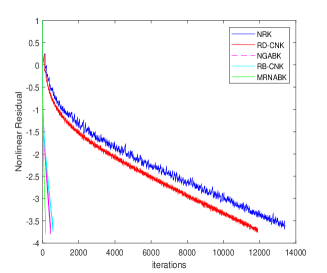
(a) $x_{0}=zero(100,1)$

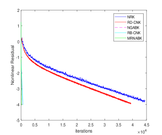
(b) $x_{0}=zero(300,1)$

Figure 1: H-equation at different initial value.

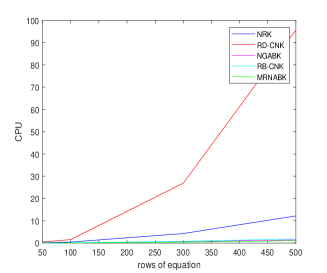
(a) CPU

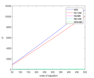
(b) IT

Figure 2: H-equation at different scales.

Example 2.

In this example, we consider the Brown almost linear function,

$$f_{k}(x)=x^{(k)}+\sum_{i=1}^{n}x^{i}-(n+1), 1\leq k\leq n;$$

$$f_{k}(x)=\left(\prod\limits_{i=1}^{n}x^{(i)}\right)-1, k=n.$$

In this experiment, we set the initial value $x_{0}=0.5\ast ones(n,1)$. The number of equations and the number of unknowns is set to $50\times 50$, $100\times 100$, $150\times 150$, $200\times 200$, $250\times 250$, $300\times 300$, $350\times 350$, $400\times 400$. We list the computing time and iteration numbers of these methods respectively in Table 5 and Table 6. The results show that our new methods greatly outperform the NRK method. We observe that the iteration time of the NGABK method and the MRNABK method is almost the same in Table 6, but both of them are better than the RB-CNK method.

Table 5: IT comparison of NRK, RD-CNK, NGABK, RB-CNK, MRNABK

$m\times n$	NRK	RD-CNK	NGABK	RB-CNK	MRNABK
$50\times 50$	4660	755	1	1	1
$100\times 100$	15881	1308	1	1	1
$150\times 150$	35398	1904	1	1	1
$200\times 200$	58127	2506	1	1	1
$250\times 250$	85937	3128	1	1	1
$300\times 300$	116851	3750	1	1	1
$350\times 350$	156027	4372	1	1	1
$400\times 400$	196134	4992	1	1	1

Table 6: CPU comparison of NRK, RD-CNK, NGABK, RB-CNK, MRNABK

$m\times n$	NRK	RD-CNK	NGABK	RB-CNK	MRNABK
$50\times 50$	0.7222	0.2290	0.0024	0.0049	0.0017
$100\times 100$	2.5929	1.2108	0.0050	0.0063	0.0045
$150\times 150$	7.5696	2.7863	0.0108	0.0149	0.0112
$200\times 200$	15.4563	5.9908	0.0187	0.0250	0.0188
$250\times 250$	24.4239	11.2057	0.0321	0.0446	0.0320
$300\times 300$	35.7111	17.4006	0.0630	0.0737	0.0530
$350\times 350$	53.0089	25.8307	0.0508	0.0775	0.0476
$400\times 400$	71.1793	36.0714	0.0626	0.0982	0.0699

Example 3.

In this example, we consider the following system of equations,

$$f_{k}(x)=((3-2x_{k})x_{k}-2x_{k+1}+1)^{2}, k=1;$$

$$f_{k}(x)=((3-2x_{k})x_{k}-x_{k-1}-2x_{k+1}+1)^{2}, 1<k<n;$$

$$f_{k}(x)=((3-2x_{k})x_{k}-x_{k-1}+1)^{2}, k=n.$$

In this experiment, we set the initial value $x_{0}=(-0.5,-0.5,\dots,-0.5)^{T}$ and $n$ is the number of the equations. Singular Broyden problem is a square nonlinear system of equations, and its Jacobian matrix is singular at the solution. As can be seen from Table 7 and Table 8, the NGABK method converges faster than the other three methods in terms of the number of iteration steps and calculation time. As can be seen from Fig. 3, the residuals of MRNABK method decline the fastest, while those of NRK method decline the slowest. From Fig. 4, we can observe that the approximate solutions can be obtained by all five methods.

Table 7: IT comparison of NRK, RD-CNK, NGABK, RB-CNK, MRNABK

$n$	NRK	RD-CNK	NGABK	RB-CNK	MRNABK
50	1524	1440	288	374	33
500	18068	17139	4531	6841	33
700	25707	24413	4357	10044	34
900	33508	31876	4867	13045	33
1500	57340	54586	13502	22743	34
2000	77487	73764	12756	22528	31

Table 8: CPU comparison of NRK, RD-CNK, NGABK, RB-CNK, MRNABK

$n$	NRK	RD-CNK	NGABK	RB-CNK	MRNABK
50	0.9005	0.4328	0.1038	0.1824	0.0422
500	3.8890	6.7895	1.9450	3.0060	0.6040
700	6.0818	12.7727	3.1249	4.8353	0.8893
900	8.9058	19.6451	4.5572	7.2238	1.2652
1500	20.2697	35.6259	11.6104	18.6458	3.1587
2000	32.7492	71.2359	19.3939	33.8771	4.6496

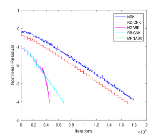
(a) $n=500$

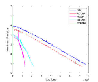
(b) $n=2000$

Figure 3: Singular Broyden problem with n = 500 (left), 2000 (right).

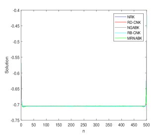
(a) $n=500$

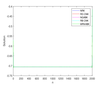
(b) $n=2000$

Figure 4: Singular Broyden problem’s solution with n = 500 (left), 2000 (right).

Example 4.

Consider the following overdetermined nonlinear problem,

$$f_{k}(x)=10\left(\frac{2x_{i}}{(1+(x_{i})^{2})^{2}}-x_{i+1}\right), \quad mod(k,2)=1,$$

$$f_{k}(x)=x_{i}-1, \quad mod(k,2)=0,$$

$$m=2(n-1), \quad i=div(k+1,2),$$

where m represents the number of equations. In this experiment, we set the initial value $x_{0}=(0,0,\dots,0)$ and $n=$ 100, 300, 500, 1000, 2000, respectively. From Table 9, we can see that NRK achieves the worst numerical result compared with the other four methods. Further, we observe that RB-CNK, MRNABK and NGABK achieve the same result in terms of the number of iterations. From Table 10, NGABK and MRNABK are slightly faster than RB-CNK in terms of iteration time, so our approach is generally effective.

Table 9: IT comparison of NRK, RD-CNK, NGABK, RB-CNK, MRNABK

$n$	NRK	RD-CNK	NGABK	RB-CNK	MRNABK
100	138	124	2	2	2
300	435	328	2	2	2
500	706	517	2	2	2
1000	1472	1042	2	2	2
2000	2829	2042	2	2	2

Table 10: CPU comparison of NRK, RD-CNK, NGABK, RB-CNK, MRNABK

$n$	NRK	RD-CNK	NGABK	RB-CNK	MRNABK
100	0.0186	0.0482	0.0094	0.0131	0.0085
300	0.1510	0.2999	0.0664	0.0709	0.0357
500	0.2273	0.3888	0.0896	0.1357	0.0836
1000	0.5298	0.9602	0.2230	0.9057	0.2019
2000	1.8300	3.8600	0.9893	5.4136	0.7435

6 Conclusion

In this paper, based on the Gaussian Kaczmarz method and RD-CNK method, we propose a new class of nonlinear Kaczmarz block methods to solve nonlinear equations and study their convergence theories. These methods use the average technique instead of calculating the Moore-Penrose pseudoinverse of the Jacobian matrix, which greatly reduces the amount of computation. Numerical results show that the NGABK method and the MRNABK method perform well in the case of singular Jacobian matrix and overdetermined equations. The study of the pseudoinverse-free method and the more efficient greedy rules is very meaningful, and this is what we need to continue to work on in the future.

References

- [1] Qipin Chen and Wenrui Hao. A homotopy training algorithm for fully connected neural networks. Proceedings of the Royal Society A, 475(2231):20190662, 2019.
- [2] James M Ortega and Werner C Rheinboldt. Iterative Solution of Nonlinear Equations in Several Variables. SIAM, 2000.
- [3] Kenji Kawaguchi. Deep Learning without Poor Local Minima. Advances in neural information processing systems, 29, 2016.
- [4] S. Kaczmarz. Angenaherte auflosung von systemen linearer glei-chungen. Bull. Int. Acad. Pol. Sic. Let., Cl. Sci. Math. Nat., pages 355–357, 1937.
- [5] Thomas Strohmer and Roman Vershynin. A Randomized Kaczmarz Algorithm with Exponential Convergence. Journal of Fourier Analysis and Applications, 15(2):262, 2009.
- [6] Anna Ma, Deanna Needell, and Aaditya Ramdas. Convergence Properties of the Randomized Extended Gauss–Seidel and Kaczmarz Methods. SIAM Journal on Matrix Analysis and Applications, 36(4):1590–1604, 2015.
- [7] Kui Du and Xiao-Hui Sun. A doubly stochastic block Gauss–Seidel algorithm for solving linear equations. Applied Mathematics and Computation, 408:126373, 2021.
- [8] Ji Liu and Stephen Wright. An accelerated randomized Kaczmarz algorithm. Mathematics of Computation, 85(297):153–178, 2016.
- [9] Yonina C Eldar and Deanna Needell. Acceleration of randomized Kaczmarz method via the Johnson–Lindenstrauss Lemma. Numerical Algorithms, 58:163–177, 2011.
- [10] Kui Du, Wu-Tao Si, and Xiao-Hui Sun. Randomized Extended Average Block Kaczmarz for Solving Least Squares. SIAM Journal on Scientific Computing, 42(6):A3541–A3559, 2020.
- [11] Anastasios Zouzias and Nikolaos M Freris. Randomized Extended Kaczmarz for Solving Least Squares. SIAM Journal on Matrix Analysis and Applications, 34(2):773–793, 2013.
- [12] Deanna Needell. Randomized Kaczmarz solver for noisy linear systems. BIT Numerical Mathematics, 50:395–403, 2010.
- [13] Kui Du and Xiao-Hui Sun. Pseudoinverse-free randomized block iterative algorithms for consistent and inconsistent linear systems. arXiv preprint arXiv:2011.10353, 2020.
- [14] Michael Griebel and Peter Oswald. Greedy and randomized versions of the multiplicative Schwarz method. Linear Algebra and its Applications, 437(7):1596–1610, 2012.
- [15] Julie Nutini, Behrooz Sepehry, Issam Laradji, Mark Schmidt, Hoyt Koepke, and Alim Virani. Convergence Rates for Greedy Kaczmarz Algorithms, and Faster Randomized Kaczmarz Rules Using the Orthogonality Graph. arXiv preprint arXiv:1612.07838, 2016.
- [16] Zhong-Zhi Bai and Wen-Ting Wu. On Greedy Randomized Kaczmarz Method for Solving Large Sparse Linear Systems. SIAM Journal on Scientific Computing, 40(1):A592–A606, 2018.
- [17] Tommy Elfving. Block-iterative methods for consistent and inconsistent linear equations. Numerische Mathematik, 35:1–12, 1980.
- [18] Jia-Qi Chen and Zheng-Da Huang. On the error estimate of the randomized double block Kaczmarz method. Applied Mathematics and Computation, 370:124907, 2020.
- [19] Deanna Needell, Ran Zhao, and Anastasios Zouzias. Randomized block Kaczmarz method with projection for solving least squares. Linear Algebra and its Applications, 484:322–343, 2015.
- [20] Deanna Needell and Joel A Tropp. Paved with good intentions: Analysis of a randomized block Kaczmarz method. Linear Algebra and its Applications, 441:199–221, 2014.
- [21] Ion Necoara. Faster randomized block Kaczmarz algorithms. SIAM Journal on Matrix Analysis and Applications, 40(4):1425–1452, 2019.
- [22] A-Qin Xiao, Jun-Feng Yin, and Ning Zheng. On fast greedy block Kaczmarz methods for solving large consistent linear systems. Computational and Applied Mathematics, 42(3):119, 2023.
- [23] Robert M Gower and Peter Richtárik. Randomized Iterative Methods for Linear Systems. SIAM Journal on Matrix Analysis and Applications, 36(4):1660–1690, 2015.
- [24] Qifeng Wang, Weiguo Li, Wendi Bao, and Xingqi Gao. Nonlinear Kaczmarz algorithms and their convergence. Journal of Computational and Applied Mathematics, 399:113720, 2022.
- [25] Wen-Jun Zeng and Jieping Ye. Successive Projection for Solving Systems of Nonlinear Equations/Inequalities. arXiv preprint arXiv:2012.07555, 2020.
- [26] Yanjun Zhang and Hanyu Li. Greedy capped nonlinear Kaczmarz methods. arXiv preprint arXiv:2210.00653, 2022.
- [27] Jianhua Zhang, Yuqing Wang, and Jing Zhao. On maximum residual nonlinear Kaczmarz-type algorithms for large nonlinear systems of equations. Journal of Computational and Applied Mathematics, page 115065, 2023.
- [28] Yanjun Zhang, Hanyu Li, and Ling Tang. Greedy randomized sampling nonlinear Kaczmarz methods. arXiv preprint arXiv:2209.06082, 2022.
- [29] Rui Yuan, Alessandro Lazaric, and Robert M Gower. Sketched Newton-Raphson. SIAM Journal on Optimization, 32(3):1555–1583, 2022.