Kernel Methods are Competitive for Operator Learning

Abstract

We present a general kernel-based framework for learning operators between Banach spaces along with a priori error analysis and comprehensive numerical comparisons with popular neural net (NN) approaches such as Deep Operator Networks (DeepONet) [46] and Fourier Neural Operator (FNO) [45]. We consider the setting where the input/output spaces of target operator $\mathcal{G}^{\dagger}\,:\,\mathcal{U}\to\mathcal{V}$ are reproducing kernel Hilbert spaces (RKHS), the data comes in the form of partial observations $\phi(u_{i}),\varphi(v_{i})$ of input/output functions $v_{i}=\mathcal{G}^{\dagger}(u_{i})$ ($i=1,\ldots,N$), and the measurement operators $\phi\,:\,\mathcal{U}\to\mathbb{R}^{n}$ and $\varphi\,:\,\mathcal{V}\to{\mathbb{R}}^{m}$ are linear. Writing $\psi\,:\,\mathbb{R}^{n}\to\mathcal{U}$ and $\chi\,:\,\mathbb{R}^{m}\to\mathcal{V}$ for the optimal recovery maps associated with $\phi$ and $\varphi$, we approximate $\mathcal{G}^{\dagger}$ with $\bar{\mathcal{G}}=\chi\circ\bar{f}\circ\phi$ where $\bar{f}$ is an optimal recovery approximation of $f^{\dagger}:=\varphi\circ\mathcal{G}^{\dagger}\circ\psi\,:\,\mathbb{R}^{n}\to\mathbb{R}^{m}$. We show that, even when using vanilla kernels (e.g., linear or Matérn), our approach is competitive in terms of cost-accuracy trade-off and either matches or beats the performance of NN methods on a majority of benchmarks. Additionally, our framework offers several advantages inherited from kernel methods: simplicity, interpretability, convergence guarantees, a priori error estimates, and Bayesian uncertainty quantification. As such, it can serve as a natural benchmark for operator learning.

1 Introduction

Operator learning is a well-established field going back at least to the 1970s with the articles [1, 56] who introduced the reduced basis method as a way speeding up expensive model evaluations. In the most broad sense operator learning arises in the solution of stochastic PDEs [28], emulation of computer codes [37], reduced order modeling (ROM) [48], and numerical homogenization [61]. In recent years, and with the rise of machine learning, operator learning has become the focus of extensive research with the development of neural net (NN) methods such as Deep Operator Nets [46] and Fourier Neural Nets [45] among many others. While these NN methods are often benchmarked against each other [47], they are rarely compared with the aforementioned classical approaches. Furthermore, the theoretical analysis of NN methods is often limited to density/universal approximation results; showing the existence of a network of a requisite size achieving a certain error rate, without guarantees whether this network is computable in practice (see for example [20, 41]).

In order to alleviate the aforementioned shortcomings we present a mathematical framework for approximation of mappings between Banach spaces using the theory of operator valued reproducing Kernel Hilbert spaces (RKHS) and Gaussian Processes (GPs). Our abstract framework is: (1) mathematically simple and interpretable, (2) convenient to implement, (3) encompasses some of the classical approaches such as linear methods; and (4) comes with a priori error analysis and convergence theory. We further present extensive benchmarking of our kernel method with the DeepONet and FNO approaches and show that the kernel approach either matches or outperforms NN methods in most benchmark examples.

In the remainder of this section we give a summary of our methodology and results: We pose the operator learning problem in Section 1.1 before presenting a running example in Section 1.2 which is used to outline our proposed framework and main theoretical results in Sections 1.3 and 1.4 as well as brief numerical results in Section 1.5. Our main contributions are summarized in Section 1.6 followed by a literature review in Section 1.7.

1.1 The operator learning problem

Let $\mathcal{U}$ and $\mathcal{V}$ be two (possibly infinite-dimensional) separable Banach spaces and suppose that

(1) $${\mathcal{G}}^{\dagger}:\mathcal{U}\to\mathcal{V}\,$$

is an arbitrary (possibly nonlinear) operator. Then, broadly speaking, the goal of operator learning is to approximate ${\mathcal{G}}^{\dagger}$ from a finite number $N$ of input/output data on ${\mathcal{G}}^{\dagger}$. For our framework, we consider the setting where the input/output data are only partially observed through a finite collection of linear measurements which we formalize as follows:

Problem 1.

Let $\{u_{i},v_{i}\}_{i=1}^{N}$ be $N$ elements of $\mathcal{U}\times\mathcal{V}$ such that

(2) $${\mathcal{G}}^{\dagger}(u_{i})=v_{i},\quad\text{for }i=1,\dots,N\,.$$

Let $\phi:\mathcal{U}\to{\mathbb{R}}^{n}$ and $\varphi:\mathcal{V}\to{\mathbb{R}}^{m}$ be bounded linear operators. Given the data $\{\phi(u_{i}),\varphi(v_{i})\}_{i=1}^{N}$ approximate ${\mathcal{G}}^{\dagger}$.

1.2 Running example

To give context to the above problem and our solution method we briefly outline a running example to which the reader can refer to throughout the rest of this section. Consider the following elliptic PDE, which is of broad interest in geosciences and material science:

(3) $$\left\{\begin{aligned} -\text{div}\>e^{u}\>\nabla v&=w,&&\text{in}\quad\Omega,\\ v&=0,&&\text{on}\quad\partial\Omega\,.\end{aligned}\right.$$

where $\Omega=(0,1)^{2}$, $u\in H^{3}(\Omega)$, $w\in H^{1}(\Omega)$ and $v\in H^{3}(\Omega)\cap H^{1}_{0}(\Omega)$. For a fixed forcing term $w$, we wish to approximate the nonlinear operator mapping the diffusion coefficient $u$ to the solution $v$, i.e., ${\mathcal{G}}^{\dagger}:u\mapsto v$. In this case we may take $\mathcal{U}\equiv H^{3}(\Omega)$ and $\mathcal{V}\equiv H^{3}(\Omega)\cap H^{1}_{0}(\Omega)$. We further assume that a training data set is available in the form of limited observations of input-out pairs. As a canonical example, consider the evaluation bounded and linear operators

(4) $$\phi:u\mapsto\left(u(X_{1}),u(X_{2}),\dots,u(X_{n})\right)^{T}\quad\text{and}\quad\varphi:v\mapsto\left(v(Y_{1}),v(Y_{2}),\dots,v(Y_{m})\right)^{T},$$

where the $\{X_{j}\}_{j=1}^{n}$ and $\{Y_{j}\}_{j=1}^{m}$ are distinct collocation points in the domain $\Omega$ as well as pairs $\{u_{i},v_{i}\}_{i=1}^{N}$ that satisfy the PDE (3). Then our goal is to approximate ${\mathcal{G}}^{\dagger}$ from the training data set $\{\phi(u_{i}),\varphi(v_{i})\}_{i=1}^{N}$ .

1.3 The proposed solution

Our setup naturally gives rise to a commutative diagram depicted in Figure 1. Here the map $f^{\dagger}:{\mathbb{R}}^{n}\to{\mathbb{R}}^{m}$ explicitely defined as

(5) $$f^{\dagger}:=\varphi\circ{\mathcal{G}}^{\dagger}\circ\psi$$

is a mapping between finite-dimensional Euclidean spaces, and is therefore amenable to numerical approximation. However, in order to approximate ${\mathcal{G}}^{\dagger}$ we also need the reconstruction maps $\psi:{\mathbb{R}}^{n}\to\mathcal{U}$ and $\chi:{\mathbb{R}}^{m}\to\mathcal{V}$.

Figure 1: Commutative diagram of our operator learning setup.

Our proposed solution is to endow $\mathcal{U}$ and $\mathcal{V}$ with an RKHS structure and use kernel/GP regression to identify the maps $\psi$ and $\chi$. As a prototypical example we consider the situation where $\mathcal{U}$ is an RKHS of functions $u\,:\,\Omega\to{\mathbb{R}}$ defined by a kernel $Q\,:\,\Omega\times\Omega\rightarrow{\mathbb{R}}$ and $\mathcal{V}$ is an RKHS of functions $u\,:\,D\to{\mathbb{R}}$ defined by a kernel $K\,:\,D\times D\rightarrow{\mathbb{R}}$. For our running example, we have $D=\Omega$, and we can take $Q$ and $K$ to be Matérn like kernels, e.g., the Green’s function of elliptic PDEs (possibly on $\Omega$ or restricted to $\Omega$) with appropriate regularity. One can also choose $Q,K$ to be smoother kernels such that their RKHSs are embedded in $\mathcal{U}$ and $\mathcal{V}$.

We then define $\psi$ and $\chi$ as the following optimal recovery maps :

(6) $$\psi(U) :=\operatorname*{arg\,min}_{w\in\mathcal{U}}\|w\|_{Q}\quad\text{s.t.}\quad\phi(w)=U,$$

$$\chi(V) :=\operatorname*{arg\,min}_{w\in\mathcal{V}}\|w\|_{K}\quad\text{s.t.}\quad\varphi(w)=V,$$

where $\|\cdot\|_{Q}$ and $\|\cdot\|_{K}$ are the RKHS norms arising from their pertinent kernels.

In the case where $\phi$ and $\varphi$ are pointwise evaluation maps ($\phi(u)=(u(X_{1}),\ldots,u(X_{n}))$ and $\varphi(v)=(v(Y_{1}),\ldots,v(Y_{m}))$ where the $X_{i}$ and $Y_{j}$ are pairwise distinct collocation points in $\Omega$ and $D$), our optimal recovery maps can be expressed in closed form using standard representer theorems for kernel interpolation [71]:

(7) $$\psi(U)(x)=Q(x,X)Q(X,X)^{-1}U,\qquad\chi(V)(y)=K(y,Y)K(Y,Y)^{-1}V,$$

where $Q(X,X)$ and $K(Y,Y)$ are kernel matrices with entries $Q(X,X)_{ij}=Q(X_{i},X_{j})$ and $K(Y,Y)_{ij}=K(Y_{i},Y_{j})$ respectively, while $Q(x,X)$ and $K(y,Y)$ denote row-vector fields with entries $Q(x,X)_{i}=Q(x,X_{i})$ and $K(y,Y)_{i}=K(y,Y_{i})$.

We further propose to approximate $f^{\dagger}$ by optimal recovery in a vector-valued RKHS. Let $\Gamma\,:\,{\mathbb{R}}^{n}\times{\mathbb{R}}^{n}\to{\mathcal{L}}({\mathbb{R}}^{m})$ be a matrix valued kernel [3]; here ${\mathcal{L}}({\mathbb{R}}^{m})$ is the space of $m\times m$ matrices) with RKHS $\mathcal{H}_{\Gamma}$ equipped with the norm $\|\cdot\|_{\Gamma}$ and proceed to approximate $f^{\dagger}$ by the map $\bar{f}$ defined as

$$\bar{f}:=\operatorname*{arg\,min}_{f\in\mathcal{H}_{\Gamma}}\|f\|_{\Gamma}\quad\text{s.t.}\quad f(\phi(u_{i}))=\varphi(v_{i})\quad\text{for}\quad i=1,\dots,N.$$

A simple and practical choice for $\Gamma$ is the diagonal kernel

(8) $$\Gamma(U,U^{\prime})=S(U,U^{\prime})I$$

where $S:{\mathbb{R}}^{n}\times{\mathbb{R}}^{n}\to{\mathbb{R}}$ is an arbitrary scalar-valued kernel, such as RBF, Laplace, or Matérn, and $I$ is the $m\times m$ identity matrix. More complicated choices, such as sums of kernels or replacing the identity matrix for a fixed positive definite matrix, implying correlations between various input or output correlations, are also possible. However, these may lead to greater computational cost and we observe empirically that the simple choice of the identity matrix already provides good performance. Then we can approximate the components of $\bar{f}$ via the independent optimal recovery problems

(9) $$\bar{f}_{j}:=\operatorname*{arg\,min}_{g\in\mathcal{H}_{S}}\|g\|_{S}\quad\text{s.t.}\quad g(\phi(u_{i}))=\varphi_{j}(v_{i}),\quad\text{for}\quad i=1,\dots,N$$

for $j=1,\dots,m$. Here we wrote $\varphi_{j}(v_{i})$ for the entry $j$ of the vector $\varphi(v_{i})$ and, as our notation suggests, $\mathcal{H}_{S}$ is the RKHS of $S$ equipped with the norm $\|\cdot\|_{S}$. Since (9) is a standard optimal recovery problem, each $\bar{f}_{j}$ can be identified by the usual representer formula:

(10) $$\bar{f}_{j}(U)=S(U,{\bf{U}})S({\bf{U}},{\bf{U}})^{-1}{\bf{V}}_{\cdot,j},$$

where ${\bf{U}}:=(\phi(u_{1}),\dots,\phi(u_{N}))$ and ${\bf{V}}_{\cdot,j}:=(\varphi_{j}(v_{1}),\dots,\varphi_{j}(v_{N}))^{T}$ and $S(U,{\bf{U}})$ is a block-vector and $S({\bf{U}},{\bf{U}})$ is a block-matrix defined in an analogous manner to those in (7). By combining equations (7) and (10) we obtain the operator

(11) $$\bar{{\mathcal{G}}}:=\chi\circ\bar{f}\circ\phi$$

as an approximation to ${\mathcal{G}}^{\dagger}$. We provide further details and generalize the proposed framework in Section 2 to the setting where $\phi$ and $\varphi$ are obtained from arbitrary linear measurements (e.g., integral operators as in tomography) and $\mathcal{U}$ and $\mathcal{V}$ may not be spaces of continuous functions.

1.4 Convergence guarantee

Under suitable regularity assumptions on ${\mathcal{G}}^{\dagger}$, our method comes with worst-case convergence guarantees as the number of data points $N$ , i.e., input-output pairs and the number of collocations points $n$ and $m$ go to infinity. We present here a condensed version of this result and defer the proof to Section 3. Below we write $B_{R}(\mathcal{H})$ for the ball of radius $R>0$ in a normed space ${\mathcal{H}}$.

Theorem 1.1 (Condensed version of Thm. 3.8).

Suppose it holds that:

1. (Regularity of the domains $\Omega$ and $D$) $\Omega$ and $D$ are compact sets of finite dimensions $d_{\Omega}$ and $d_{D}$ and with Lipschitz boundary.

2. Regularity of the kernels $Q$ and $K$. Assume that $\mathcal{H}_{Q}\subset H^{s}(\Omega)$ and $\mathcal{H}_{K}\subset H^{t}(D)$ for some $s>d_{\Omega}/2$ and some $t>d_{D}/2$ with inclusions indicating continuous embeddings.

3. (Space filling property of collocation points)The fill distance between the collocation points $\{X_{i}\}_{i=1}^{n}\subset\Omega$ and the $\{Y_{j}\}_{j=1}^{m}\subset D$ goes to zero as $n\rightarrow\infty$ and $m\rightarrow\infty$.

4. (Regularity of the operator ${\mathcal{G}}^{\dagger}$) The operator ${\mathcal{G}}^{\dagger}$ is continuous from $H^{s^{\prime}}(\Omega)$ to ${\mathcal{H}}_{K}$ for some $s^{\prime}\in(0,s)$ as well as from $\mathcal{U}$ to $\mathcal{V}$ and all its Fréchet derivatives are bounded on $B_{R}(\mathcal{H}_{Q})$ for any $R>0$.

5. (Regularity of the kernels $S^{n}$) Assume that for any $n\geq 1$ and any compact subset $\Upsilon$ of ${\mathbb{R}}^{n}$, the RKHS of $S^{n}$ restricted to $\Upsilon$ is contained in $H^{r}(\Upsilon)$ for some $r>n/2$ and contains $H^{r^{\prime}}(\Upsilon)$ for some $r^{\prime}>0$ that may depend on $n$.

6. (Resolution and space-filling property of the data) Assume that for $n$ sufficiently large, the data points $(u_{i})_{i=1}^{N}\subset B_{R}(\mathcal{H}_{Q})$ belong to the range of $\psi^{n}$ and are space filling in the sense that they become dense in $\phi^{n}(B_{R}(\mathcal{H}_{Q}))$ as $N\rightarrow\infty$.

Then, for all $t^{\prime}\in(0,t)$,

(12) $$\lim_{n,m\rightarrow\infty}\lim_{N\rightarrow\infty}\sup_{u\in B_{R}(\mathcal{H}_{Q})}\|{\mathcal{G}}^{\dagger}(u)-\chi^{m}\circ\bar{f}^{m,n}_{N}\circ\phi^{n}(u)\|_{H^{t^{\prime}}(D)}\to 0\,,$$

where our notation makes the dependence of $\psi,\phi,\chi,S$ and $\bar{f}$ on $n,m$ and $N$ explicit.

We note that Assumptions (1.1.1)–(1.1.3) are standard, and concern the accuracy of the optimal recovery maps $\phi^{n}$ and $\chi^{m}$ as $n,m\to\infty$. Assumptions (1.1.4)–(1.1.5) are less standard and amount to regularity assumptions on the map ${\mathcal{G}}^{\dagger}$ while Assumption (1.1.6) concerns the acquisition and regularity of the training data set.

In Section 3 we also present Theorem 3.5 as the quantitative analogue of the above result which characterizes how the speed of convergence depends on the regularity of the operator ${\mathcal{G}}^{\dagger}$ and the choice of $\phi$ and $\varphi$ in the setting of pointwise measurement operators. We also comment on how this analysis could be extended to other linear measurements.

1.5 Numerical Framework

Returning to our running example, we implement the proposed framework for learning the non-linear operator mapping $u$ to $v$ in (3). We consider 1000 inputs and outputs of $u$ and $v$. The data is taken from [47] and the experimental setup is discussed further in Section 4.3.2. We take $\varphi$ to be of the form (4) with $m=841$ while we define $\phi$ through a PCA pre-processing step. More precisely, let $\phi_{\text{pointwise}}$ be of the form (4) with $n=841$. Choose $n_{\text{PCA}}=202$ (this value captures $95\%$ of the empirical variance of our training data) and define

(13) $$\phi(u)=\Pi_{\text{PCA}}\circ\phi_{\text{pointwise}}(u)\in{\mathbb{R}}^{202}.$$

In other words, we take our $\phi$ map to be the linear map that computes the first 202 PCA coefficients of the input functions $u$ given on a uniform grid; observe that we do not use PCA pre-processing on the output data here although we do this for some of our other examples in Section 4 for better performance.

With $\phi$ and $\varphi$ identified (recall Figure 1) we proceed to implement our kernel method using the simple choice of a diagonal kernel $S(U,U^{\prime})I$ where $S$ is a rational quadratic (RQ) kernel (see Appendix C). This choice transforms the problem into $841$ independent kernel regression problems, each corresponding to one component of $f^{\dagger}$ (i.e., the $f^{\dagger}_{j}$’s).

We used the PCA and kernel regression modules of the scikit-learn Python library [65] to implement our algorithm. This implementation automatically selects the best kernel parameters by maximizing the marginal likelihood function [67] jointly for all problems. Our proposed method can therefore be implemented conveniently using off-the-shelf software. Figure 3 illustrates examples of the inputs and outputs of our operator learning problem. Despite the simple implementation of our method, we are able to obtain competitive accuracy as shown in Table 1 where the relative testing $L^{2}$ loss of our method is compared to other popular algorithms. Moreover, our approach is amenable to well-known numerical analysis techniques, such as sparse or low-rank approximation of kernel matrices, to reduce its complexity. For the present example (and those in Section 4) we only consider vanilla kernel methods which compute (10) by computing the full Cholesky factors of the matrix $S({\bf{U}},{\bf{U}})$.

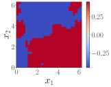
(a)

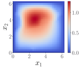
(b)

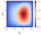
(c)

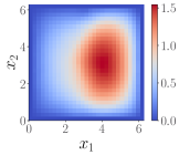
(d)

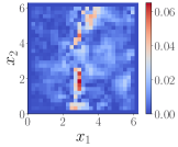
(e)

Figure 3: Example of training data and test prediction and pointwise errors for the Darcy flow problem (3).

Method	Accuracy
DeepONet	2.91 %
FNO	2.41 %
POD-DeepONet	2.32 %
Linear	6.74 %
Rational quadratic	2.87%

Table 1: The $L^{2}$ relative test error of the Darcy flow problem in our running example. The kernel approach is compared with variations of DeepONet and FNO. Results of our kernel method are presented below the dashed line with the pertinent choice of the kernel $S$.

1.6 Summary of contributions

The main results of the article concern the properties, performance, and error analysis of the map $\bar{{\mathcal{G}}}$ defined in (11). Our contributions can be summarized under four categories:

1. An abstract kernel framework for operator learning: In Section 2, we propose a framework for operator learning using kernel methods with several desirable properties. A family of methods of increasing complexity is proposed that includes linear models and diagonal kernels as well as non-diagonal kernels which capture output correlations. These properties make our approach ideal for benchmarking purposes. Furthermore, the methodology is: (i) applicable to any choice of the linear functionals $\varphi$ and $\phi$; (ii) minimax optimal with respect to an implicitly defined operator-valued kernel; and (iii) is mesh-invariant. We emphasize in Remark 2.1 that our optimal recovery maps can be applied to any operator learning after training to obtain a mesh-invariant pipeline.

2. Error analysis and convergence rates for $\bar{{\mathcal{G}}}$: In Section 3, we develop rigorous worst-case a priori error bounds and convergence guarantees for our method: Theorem 3.5 provides quantitative error bounds while Theorem 3.8 (the detailed version of Theorem 3.5) shows the convergence of $\bar{{\mathcal{G}}}\to{\mathcal{G}}$ under appropriate conditions.

3. A simple to use vanilla kernel method: While our abstract kernel method is quite general, our numerical implementation in Section 4 focuses on a simple, easy-to-implement version using diagonal kernels of the form (8). Off-the-shelf software, such as the kernel regression modules of scikit-learn, can be employed for this task. We empirically observe low training times and robust choice of hyperparameters. These properties further suggest that kernel methods are a good baseline for benchmarking of more complex methods.

4. Competitive performance. In Section 4 we present a series of numerical experiments on benchmark PDE problems from the literature and observe that our simple implementation of the kernel approach is competitive in terms of complexity-accuracy tradeoffs in comparison to several NN-based methods. Since kernel methods can be interpreted as an infinite-width, one-layer NN, the results raise the question of how much of a role the depth of a deep NN plays in the performance of algorithms for the purposes of operator learning.

1.7 Review of relevant literature

In the most broad sense, operator learning is the problem of approximating a mapping between two infinite-dimensional function spaces [9, 19]. In recent years, this problem has become an area of intense research in the scientific machine learning community with a particular focus on parametric or stochastic PDEs. However, the approximation of such parameter to solution maps has been an area of intense research in the computational mathematics and engineering communities, going back at least to the reduced basis method introduced in the 1970s [1, 56] as a way of speeding up the solution of families of parametric PDEs in applications that require many PDE solves such as design [21, 52, 8, 10], uncertainty quantification (UQ) [72, 51, 35], and multi-scale modeling [76, 27, 26, 42]. In what follows we give a brief summary of the various areas and methodologies that overlap with operator learning; we cannot provide an exhaustive list of references due to space, but refer the reader to key contributions and surveys where further references can be found.

Deep learning techniques

The use of NNs for operator learning goes back at least to the 90s and the seminal works of Chen and Chen [13, 12] who proved a universal approximation theorem for NN approximations to operators. The use and design of NNs for operator learning has become popular in the last five years as a consequence of growing interest in NNs for scientific computing starting with the article [81] which used autoencoders to build surrogates for UQ of subsurface flow models. Since then many different approaches have been proposed some of which use specific architectures or target particular families of PDEs [33, 39, 45, 38, 46, 29, 11, 44, 40]. The most relevant of among these methods to our proposed framework are the DeepONet family [46, 74, 47, 75], FNO [45], and PCA-Net [33, 9] where the main novelty appears to be the use of novel, flexible, and expressive NN architectures that allow the algorithm to learn and adapt the bases that are selected for the input and outputs of the solution map as well as possible nonlinear dependencies between the basis coefficients. Although not part of our comparisons, we note that [22, 23, 24] obtained competitive accuracy by using deep neural networks with architectures inspired by conventional fast solvers.

Classical numerical approximation methods

Operator learning has been the subject of intense research in the computational mathematics literature in the context of stochastic Galerkin methods [28, 80], polynomial chaos [78, 79], reduced basis methods [56, 49] and numerical homogenization [63, 57, 61, 2]. In the setting of stochastic and parametric PDEs, the the goal is often to approximate the solution of a PDE as a function of a random or uncertain parameter. The well-established approach to such problems is to pick or construct appropriate bases for the input parameter and the solution of the PDE and then construct a parametric, high-dimensional map, that transforms the input basis coefficients to the output coefficients. Well-established methods such as polynomial chaos, stochastic finite element methods, reduced basis methods [28, 78, 18, 34, 48] fall within this category. A vast amount of literature in applied mathematics exists on this subject, and the theoretical analysis of these methods is extensive; see for example [7, 16, 17, 55, 54, 30] and references therein.

Operator compression

For solving PDEs, the objectives of operator learning are also similar to those of operator compression [25, 44] as formulated in numerical homogenization [61, 2] and reduced order modeling (ROM) [4, 48], i.e., the approximation of the solution operator from pairs of solutions and source/forcing terms. While both ROM and numerical homogenization seek operator compression through the identification of reduced basis functions that are as accurate as possible (this translates into low-rank approximations with SVD and its variants [11]), numerical homogenization also requires those functions to be as localized as possible [50] and in turn leverages both low rank and sparse approximations. These localized reduced basis functions are known as Wannier functions in the physics literature [53], and can be interpreted as linear combinations of eigenfunctions that are localized in both frequency space and the physical domain, akin to wavelets. The hierarchical generalization of numerical homogenization [58] (gamblets) has led to the current state-of-the-art for operator compression of linear elliptic [68, 70] and parabolic/hyperbolic PDEs [64]. In particular, for arbitrary (and possibly unknown) elliptic PDEs [69] shows that the solution operator (i.e., the Green’s function) can be approximated in near-linear complexity to accuracy $\epsilon$ from only $\mathcal{O}(\log^{d+1}(\frac{1}{\epsilon}))$ solutions of the PDE.

GP emulators

In the case where the range of the operator of interest is finite dimensional, then operator learning coincides with surrogate modeling techniques that were developed in the UQ literature, such as GP surrogate modeling/emulation [37, 6]. When the kernels of the underlying GPs are also learned from data [62, 15], GP surrogate modeling has been shown to offer a simple, low-cost, and accurate solution to learning dynamical systems [32], geophysical forecasting [31], and radiative transfer emulation [73], and the inference of the structure of convective storms from passive microwave observations [66]. Indeed, our proposed kernel framework for operator learning can be interpreted as an extension of these well-established GP surrogates to the setting where the range of the operator is a function space.

1.8 Outline of the article

The remainder of the article is organized as follows: We present our operator learning framework in Section 2 for the generalized setting where $\phi,\varphi$ can be any collection of bounded and linear operators along with an interpretation of our method from the GP perspective. Our convergence analysis and quantitative error bounds are presented in Section 3 where we present the full version of Theorem 3.8. Our numerical experiments, implementation details, and benchmarks against FNO and DeepONet are collected in Section 4. We discuss future directions and open problems in Section 5. The appendix collects a review of operator valued kernels and GPs along with other auxiliary details.

2 The RKHS/GP framework for operator learning

We now present our general kernel framework for operator learning, i.e., the proposed solution to Problem 1. We emphasize that here we do not require the spaces $\mathcal{U}$ and $\mathcal{V}$ to be spaces of continuous functions and in particular, we do not require the maps $\phi$ and $\varphi$ to be obtained from pointwise measurements. To describe this, we will introduce the dual spaces of $\mathcal{U}$ and $\mathcal{V}$ to define optimal recovery with respect to kernel operators rather than just kernel functions.

Write $\mathcal{U}^{\ast}$ and $\mathcal{V}^{\ast}$ for the duals of $\mathcal{U}$ and $\mathcal{V}$, and write $[\cdot,\cdot]$ for the pertinent duality pairings. Assume that $\mathcal{U}$ is endowed with a quadratic norm $\|\cdot\|_{Q}$, i.e., there exists a linear bijection $Q:\mathcal{U}^{\ast}\to\mathcal{U}$ that is symmetric ($[\phi_{a},Q\phi_{b}]=[\phi_{b},Q\phi_{a}]$), positive ($[\phi_{a},Q\phi_{a}]>0$ for $\phi_{a}\neq 0$), and such that $\|u\|^{2}_{Q}=[Q^{-1}u,u],\>\forall u\in\mathcal{U}\,.$

As in [61, Ch. 11], although $\mathcal{U}$, and $\mathcal{U}^{\ast}$ are also Hilbert spaces under $\|\cdot\|_{Q}$ and its dual norm $\|\cdot\|_{Q}^{\ast}$ (with inner products $\big{\langle}u,v\big{\rangle}_{Q}=[Q^{-1}u,v]$ and $\big{\langle}\phi_{a},\phi_{b}\big{\rangle}_{Q}^{\ast}=[\phi_{a},Q\phi_{b}]$), we will keep using the Banach space terminology to emphasize the fact that our dual pairings will not be based on the inner product through the Riesz representation theorem, but on a different realization of the dual space, as this setting is more practical.

If $\mathcal{U}$ is a space of continuous functions on a subset $\Omega\subset{\mathbb{R}}^{d_{\Omega}}$ then $\mathcal{U}^{\ast}$ contains delta Dirac functions and, to simplify notations, we also write $Q(x,y):=[\updelta_{x},Q\updelta_{y}]$ for $x,y\in{\mathbb{R}}^{d_{\Omega}}$ to denote the kernel induced by the operator $Q$. Note that in that case, $\mathcal{U}$ is a RKHS with norm $\|\cdot\|_{Q}$ induced by the kernel $Q$. Since $\phi$ is bounded and linear, its entries $\phi_{i}$ (write $\phi:=(\phi_{1},\ldots,\phi_{n})$) must be elements of $\mathcal{U}^{\ast}$. We assume those elements to be linearly independent. Write $\psi\,:\,{\mathbb{R}}^{n}\to\mathcal{U}$ for the linear operator defined by

(14) $$\psi(Y):=(Q\phi)\,Q(\phi,\phi)^{-1}Y\text{ for }Y\in{\mathbb{R}}^{n},$$

where we write $Q(\phi,\phi)$ for the $n\times n$ symmetric positive definite (SPD) matrix with entries $Q(\phi_{i},\phi_{j}):=[\phi_{i},Q\phi_{j}]$ and $Q\phi$ for $(Q\phi_{1},\ldots,Q\phi_{n})\in\mathcal{U}^{n}$. As described in [61, Chap. 11], for $u\in\mathcal{U}$, given $\phi(u)=Y$, $\psi(Y)$ is the minmax optimal recovery of $u$ when using the relative error in $\|\cdot\|_{Q}$-norm as a loss.

Similarly, assume that $\mathcal{V}$ is endowed with a quadratic norm $\|\cdot\|_{K}$, defined by the symmetric positive linear bijection $K:\mathcal{V}^{\ast}\to\mathcal{V}$. Write $\varphi:=(\varphi_{1},\ldots,\varphi_{m})$ and assume the entries of $\varphi$ to be linearly independent elements of $\mathcal{V}^{\ast}$. Using the same notations as in (14) write $\chi\,:\,{\mathbb{R}}^{m}\to\mathcal{V}$ for the linear operator defined by

(15) $$\chi(Z):=(K\varphi)\,K(\varphi,\varphi)^{-1}Z\text{ for }Z\in{\mathbb{R}}^{m}\,.$$

Then, as above, for $v\in\mathcal{V}$, given $\varphi(v)=Z$, $\chi(Z)$ is the minmax optimal recovery of $v$ when using the relative error in $\|\cdot\|_{K}$-norm as a loss.

Write ${\mathcal{L}}({\mathbb{R}}^{m})$ for the space of bounded linear operators mapping ${\mathbb{R}}^{m}$ to itself , i.e., $m\times m$ matrices. Let $\Gamma\,:\,{\mathbb{R}}^{n}\times{\mathbb{R}}^{n}\to{\mathcal{L}}({\mathbb{R}}^{m})$ be a matrix-valued kernel [3] defining an RKHS ${\mathcal{H}}_{\Gamma}$ of continuous functions $f\,:\,{\mathbb{R}}^{n}\to{\mathbb{R}}^{m}$ equipped with an RKHS norm $\|\cdot\|_{\Gamma}$. For $i\in\{1,\ldots,N\}$, write $U_{i}:=\phi(u_{i})$ and $V_{i}:=\varphi(v_{i})$. Write ${\bf{U}}$ and ${\bf{V}}$ for the block-vectors with entries $U_{i}$ and $V_{i}$. Write $\Gamma({\bf{U}},{\bf{U}})$ for the $N\times N$ block-matrix with entries $\Gamma(U_{i},U_{j})$ and assume $\Gamma(U,U)$ to be invertible (which is satisfied if $\Gamma$ is non-degenerate and $U_{i}\not=U_{j}$ for $i\not=j$). Let $f^{\dagger}$ be an element of ${\mathcal{H}}_{\Gamma}$ and write $f^{\dagger}({\bf{U}})$ for the block vector with entries $f^{\dagger}(U_{i})$. Then given $f^{\dagger}({\bf{U}})={\bf{V}}$ it follows that

(16) $$\bar{f}(U):=\Gamma(U,{\bf{U}})\Gamma({\bf{U}},{\bf{U}})^{-1}{\bf{V}}\,,$$

is the minimax optimal recovery of $f^{\dagger}$, where $\Gamma(\cdot,{\bf{U}})$ is the block-vector with entries $\Gamma(\cdot,U_{i})$.

To this end, we propose to approximate the ground truth operator ${\mathcal{G}}^{\dagger}$ with

(17) $$\bar{{\mathcal{G}}}:=\chi\circ\bar{f}\circ\phi\,,$$

also recall Figure 1. Combining (15) and (16) we further infer that $\bar{{\mathcal{G}}}$ admits the following explicit representer formula

(18) $$\bar{{\mathcal{G}}}(u)=(K\varphi)\,K(\varphi,\varphi)^{-1}\Gamma(\phi(u),{\bf{U}})\Gamma({\bf{U}},{\bf{U}})^{-1}{\bf{V}}.$$

In the remainder of this section we will provide more details and observations regarding our approximate operator $\bar{{\mathcal{G}}}$ that is useful later in Section 3 and of independent interest.

2.1 The kernel and RKHS associated with $\bar{{\mathcal{G}}}$

The explicit formula (18) suggests that the operator $\bar{{\mathcal{G}}}$ is an element of an RKHS defined by an operator-valued kernel, which we now characterize. For $u_{1},u_{2}\in\mathcal{U}$ and $v\in\mathcal{V}$ write

(19) $$G(u_{1},u_{2})v:=(K\varphi)\,(K(\varphi,\varphi))^{-1}\Gamma(\phi(u_{1}),\phi(u_{2}))(K(\varphi,\varphi))^{-1}\varphi(v).$$

It turns out that $G:\mathcal{U}\times\mathcal{U}\to{\mathcal{L}}(\mathcal{V})$ is a well-defined operator-valued kernel whose RKHS contains operators of the form $\bar{{\mathcal{G}}}$.

Proposition 2.1.

The kernel $G$ in (19) is an operator-valued kernel. Write ${\mathcal{H}}_{G}$ for its RKHS and $\|\cdot\|_{G}$ for the associated norm. Then it holds that ${\mathcal{G}}\in{\mathcal{H}}_{G}$ if and only if ${\mathcal{G}}=\chi\circ f\circ\phi$ for $f=\varphi\circ{\mathcal{G}}\circ\psi\in{\mathcal{H}}_{\Gamma}$ and $\|{\mathcal{G}}\|_{G}=\|f\|_{\Gamma}\,.$

Proof.

Since $G$ is Hermitian and positive, we deduce that $G$ is an operator-valued kernel. Indeed for $\tilde{u}_{1},\ldots,\tilde{u}_{m}\in\mathcal{U}$ and $\tilde{v}_{1},\ldots,\tilde{v}_{m}\in\mathcal{V}$, using $\big{\langle}\tilde{v}_{i},K\varphi_{s}\big{\rangle}_{K}=\varphi_{s}(\tilde{v}_{i})$ and the fact that $\Gamma$ is a matrix-valued kernel we have

(20) $$\big{\langle}\tilde{v}_{i},G(\tilde{u}_{i},\tilde{u}_{j})\tilde{v}_{j}\big{\rangle}_{K} =\varphi(\tilde{v}_{i})^{T}(K\varphi)\,(K(\varphi,\varphi))^{-1}\Gamma(\phi(\tilde{u}_{i}),\phi(\tilde{u}_{j}))(K(\varphi,\varphi))^{-1}\varphi(\tilde{v}_{j})$$

$$=\big{\langle}G(\tilde{u}_{j},\tilde{u}_{i})\tilde{v}_{i},\tilde{v}_{j}\big{\rangle}_{K}\,,$$

where we used $\big{\langle}\tilde{v}_{i},K\varphi_{s}\big{\rangle}_{K}=\varphi_{s}(\tilde{v}_{i})$ and the fact that $\Gamma$ is a matrix-valued kernel. Furthermore, summing (20), we deduce that $\sum_{i,j=1}^{m}\big{\langle}\tilde{v}_{i},G(\tilde{u}_{i},\tilde{u}_{j})\tilde{v}_{j}\big{\rangle}_{K}\geq 0$. From (19) we infer

(21) $$\sum_{j=1}^{m}G(u,\tilde{u}_{j})\tilde{v}_{j}=\chi\circ f\circ\phi(u)$$

with the function

(22) $$f(U)=\sum_{j=1}^{m}\Gamma(U,\phi(\tilde{u}_{j}))(K(\varphi,\varphi))^{-1}\varphi(\tilde{v_{j}})\,.$$

Furthermore using the reproducing property of $G$ and (20) we have $\left\|\sum_{j=1}^{m}G(u,\tilde{u}_{j})\tilde{v}_{j}\right\|_{G}^{2}=\|f\|_{\Gamma}^{2}\,.$ Therefore the closure of the space of operators of the form (21) with respect to the RKHS norm induced by $G$ is the space of functions of the form $\chi\circ f\circ\phi$ where $f$ lives in the closure of functions of the form (22) with respect to the RKHS norm induced by $\Gamma$. We deduce that ${\mathcal{H}}_{G}=\{\chi\circ f\circ\phi\mid f\in{\mathcal{H}}_{\Gamma}\}$. The uniqueness of $f$ in the representation ${\mathcal{G}}=\chi\circ f\circ\phi$ for $f\in{\mathcal{H}}_{G}$ follows from $f=\varphi\circ{\mathcal{G}}\circ\psi$ following the identities $\varphi\circ\chi=I_{d}$ and $\phi\circ\psi=I_{d}$.

Using the above result we can further characterize $\bar{{\mathcal{G}}}$ and $\bar{f}$ via optimal recovery problems in ${\mathcal{H}}_{G}$ and ${\mathcal{H}}_{\Gamma}$ respectively. In what follows we will write ${\bf{u}}$ for the $N$ vector whose entries are the $u_{i}$, and ${\mathcal{G}}({\bf{u}})$ for the $N$ vector whose entries are ${\mathcal{G}}^{\dagger}(u_{i})$.

Proposition 2.2.

The operator $\bar{{\mathcal{G}}}$ is the minimizer of

(23) $$\begin{cases}\text{Minimize }&\|{\mathcal{G}}\|_{G}^{2}\\ \text{Over }&{\mathcal{G}}\in{\mathcal{H}}_{G}\text{ such that }\varphi\circ{\mathcal{G}}({\bf{u}})=\varphi\circ{\mathcal{G}}^{\dagger}({\bf{u}})\,.\end{cases}$$

while the map $\bar{f}$ is the minimizer of

(24) $$\begin{cases}\text{Minimize }&\|f\|_{\Gamma}^{2}\\ \text{Over }&f\in{\mathcal{H}}_{\Gamma}\text{ such that }f\circ\phi({\bf{u}})=\varphi\circ{\mathcal{G}}^{\dagger}({\bf{u}})\,.\end{cases}$$

Proof.

By Proposition 2.1 $\bar{G}$ is completely identified by $\bar{f}$ and $\|\bar{G}\|_{G}=\|\bar{f}\|_{\Gamma}$. Then solving (23) is equivalent to solving (24). The statement regarding $\bar{f}$ follows directly from representer formulae for optimal recovery with matrix-valued kernels.

2.2 Regularizing $\bar{G}$ by operator regression

As is often the case with optimal recovery/kernel regression the estimator for $\bar{f}$ in (16) is susceptible to numerical error due to ill-conditioning of the kernel matrix $\Gamma({\bf{U}},{\bf{U}})$. To overcome this issue we regularize our estimator by adding a small diagonal perturbation to this matrix. More precisely, let $\gamma>0$ and write $I$ for the identity matrix. We then define the regularized map

(25) $$\bar{f}_{\gamma}(U):=\Gamma(U,{\bf{U}})\big{(}\Gamma({\bf{U}},{\bf{U}})+\gamma I\big{)}^{-1}{\bf{V}}\,.$$

This regularized map gives rise to the regularized approximate operator

$$\bar{{\mathcal{G}}}_{\gamma}:=\chi\circ\bar{f}_{\gamma}\circ\phi\,,$$

which admits the following representer formula

(26) $$\bar{{\mathcal{G}}}_{\gamma}(u)=(K\varphi)\,K(\varphi,\varphi)^{-1}\Gamma(\phi(u),{\bf{U}})\big{(}\Gamma({\bf{U}},{\bf{U}})+\gamma I\big{)}^{-1}{\bf{V}}\,.$$

We can further characterize this operator as the solution to an operator regression problem.

Proposition 2.3.

$\bar{{\mathcal{G}}}_{\gamma}$ is the solution to

(27) $$\text{Minimize }_{{\mathcal{G}}\in{\mathcal{H}}_{G}}\|{\mathcal{G}}\|_{G}^{2}+\gamma^{-1}|\varphi\circ{\mathcal{G}}({\bf{u}})-\varphi\circ{\mathcal{G}}^{\dagger}({\bf{u}})|^{2}.$$

Proof.

By Proposition 2.1, ${\mathcal{G}}=\chi\circ f\circ\phi$ solves (27) if and if $f$ solves

(28) $$\text{Minimize }_{f\in{\mathcal{H}}_{\Gamma}}\|f\|_{\Gamma}^{2}+\gamma^{-1}|f({\bf{U}})-{\bf{V}}|^{2}\,.$$

It then follows, by standard representer theorems for matrix-valued kernel regression (see Section A.5) that $\bar{f}_{\gamma}$ is the minimizer of (28).

2.3 Interpretation as conditioned operator valued GPs

Our kernel approach to operator learning has a natural GP regression interpretation that is compatible with Bayesian inference and UQ pipelines. We present some facts and observations in this direction.

Write $\xi\sim{\mathcal{N}}(0,G)$ for the centered operator-valued GP with covariance kernel $G$ and $\zeta\sim{\mathcal{N}}(0,\Gamma)$ for a centered vector valued GP with covariance kernel $\Gamma$. Then it is straightforward to show that the law of $\xi$ is equivalent to that of $\chi\circ\zeta\circ\phi$. Let $Z=(Z_{1},\dots,Z_{N})$ be a random block-vector, independent from $\xi$, with i.i.d. entries $Z_{j}\sim{\mathcal{N}}(0,\gamma I_{m})$ for $j=1,\dots,N$; here $\gamma\geq 0$ and $I_{m}$ is the $m\times m$ identity matrix.

Then $\xi$ conditioned on $\varphi\circ\xi({\bf{u}})=\varphi({\bf{v}})+Z$ is an operator-valued GP with mean $\bar{{\mathcal{G}}}_{\gamma}$, as in (26),and conditional covariance kernel

$$\begin{split}G^{\perp}&(u,u^{\prime})v=(K\varphi)\,(K(\varphi,\varphi))^{-1}\Gamma(\phi(u_{1}),\phi(u_{2}))\\ &\big{(}\Gamma(\phi(u),\phi(u^{\prime}))-\Gamma(\phi(u),{\bf{U}})(\Gamma({\bf{U}},{\bf{U}})+\gamma I)^{-1}\Gamma({\bf{U}},\phi(u^{\prime}))\big{)}(K(\varphi,\varphi))^{-1}\varphi(v)\end{split}$$

Furthermore, the law of $\xi$ conditioned on $\varphi\circ\xi({\bf{u}})=\varphi({\bf{v}})+Z$ is equivalent to that of $\chi\circ\zeta^{\perp}\circ\phi$ where $\zeta^{\perp}\sim{\mathcal{N}}(\bar{f}_{\gamma},\Gamma^{\perp})$ is the GP $\zeta$ conditioned on $\zeta({\bf{U}})={\bf{V}}+Z^{\prime}$, whose mean is $\bar{f}_{\gamma}$ as in (25) and conditional covariance kernel is

$$\Gamma^{\perp}(U,U^{\prime})=\Gamma(U,U^{\prime})-\Gamma(U,{\bf{U}})(\Gamma({\bf{U}},{\bf{U}})+\gamma I)^{-1}\Gamma({\bf{U}},U^{\prime}).$$

We also use the GP approach to derive an alternative regularization of (27) in Appendix B.

2.4 Measurement and mesh invariance

As argued in [45], mesh invariance is a key property for operator learning methods, i.e, the learned operator should be generalizable at test time beyond the specific discretization that was used during training. In our framework, this translates to being able to predict the output of a test input function $\tilde{u}$ given only a linear measurement $\tilde{\phi}(\tilde{u})$, where $\tilde{\phi}$ was unknown at training time. For example $\tilde{\phi}$ could be of the same form as $\phi$ (say (4)) but on a finer or coarser grid. Similarly, we may choose to output with an operator $\tilde{\varphi}$ which is a coarse/fine version of $\varphi$. Our proposed framework can easily provide mesh invariance using additional optimal recovery and measurement operators at the input and outputs of the operator $\bar{{\mathcal{G}}}$ as depicted in Figure 4. In fact, we can not only accommodate modification of the grid but completely different measurement operators at testing time. For example, while $\phi,\varphi$ may be of the form (4) we may take $\tilde{\phi}$ and $\tilde{\varphi}$ to be integral operators such as Fourier or Radon transforms.

Let us describe our approach to mesh invariance in detail. Given bounded and linear operators $\tilde{\phi}:\mathcal{U}\to{\mathbb{R}}^{\tilde{n}}$ and $\tilde{\varphi}:\mathcal{V}\to{\mathbb{R}}^{\tilde{m}}$ we can approximate $\tilde{\varphi}(\mathcal{G}^{\dagger}(\tilde{u}))$ using the map $\bar{f}$ obtained from (16) defined in terms of our training. To achieve mesh invariance we simply need a consistent approach to interpolate/extend the testing measurment operators to those used for training and we achieve this using the optimal recovery map $\tilde{\psi}$ that is defined from $\tilde{\phi}$ analogously to $\psi$ in (14). This setup gives rise to a natural approximation of ${\mathcal{G}}^{\dagger}$ in terms of the function $h^{\dagger}:{\mathbb{R}}^{\tilde{n}}\to\mathbb{R}^{\tilde{m}}$ depicted in Figure 4 which in turn can be approximated with $\bar{h}:=\tilde{\varphi}\circ\chi\circ\bar{f}\circ\phi\circ\tilde{\psi}\equiv\tilde{\varphi}\circ\bar{{\mathcal{G}}}\circ\tilde{\psi}$. This expression further gives rise to another approximation to ${\mathcal{G}}^{\dagger}$ given by the operator $\tilde{{\mathcal{G}}}=\tilde{\chi}\circ\bar{h}\circ\tilde{\phi}$.

Remark 2.1.

Observe that the definition of $\bar{h}$ (and consequently $\bar{{\mathcal{G}}}$) is independent of the fact that $\bar{f}$ is constructed using the kernel approach. Thus, the optimal recovery maps $\chi$ and $\tilde{\psi}$ can be used to retrofit any fixed-mesh operator learning algorithm, to become mesh-invariant and able to use arbitrary linear measurements of the function $\tilde{u}$ at test time.

Figure 4: Generalization of Fig. 1 to the mesh invariant setting where the measurement functionals are different at test time.

3 Convergence and error analysis

In this section, we present convergence guarantees and rigorous a priori error bounds for our proposed kernel method for operator learning and give a detailed statement and proof of Theorem 3.5. We assume that ${\mathcal{H}}_{Q}$ is a space of continuous functions from $\Omega\subset{\mathbb{R}}^{d_{\Omega}}$ and that ${\mathcal{H}}_{K}$ is a space of continuous functions from $D\subset{\mathbb{R}}^{d_{D}}$. Abusing notations we write $Q:\Omega\times\Omega\to\mathbb{R}^{d_{\Omega}}$ and $K:D\times D\to\mathbb{R}^{d_{D}}$ for the kernels induced by the operators $Q$ and $K$. Let $X=(X_{1},\dots,X_{n})\subset\Omega$ and $Y=(Y_{1},\dots,Y_{m})\subset D$ be distinct collections of points and define their fill-distances

$$h_{X}:=\max_{x^{\prime}\in\Omega}\min_{x\in X}|x-x^{\prime}|,\qquad h_{Y}:=\max_{y^{\prime}\in D}\min_{y\in Y}|y-y^{\prime}|.$$

This section focuses on operators $\phi$ and $\varphi$ that are linear combinations of pointwise measurements in $X$ and $Y$. The presented results can be extended by using analogs of the sampling inequalities for other linear measurements, see [61, Theorem 4.11, Lemma 14.34] for a general framework that allows one to obtain such inequalities.

Let $L_{Q}$ and $L_{K}$ be invertible $n\times n$ and $m\times m$ matrices. For $u\in{\mathcal{H}}_{Q}$ write $u(X)$ for the $n$-vector with entries $u(X_{i})$ and let $\phi\,:\,{\mathcal{H}}_{Q}\to{\mathbb{R}}^{n}$ be the bounded linear map defined by

(29) $$\phi(u)=L_{Q}u(X)\,.$$

For $v\in{\mathcal{H}}_{K}$ write $v(Y)$ for the $m$-vector with entries $v(Y_{j})$ and let $\varphi\,:\,{\mathcal{H}}_{K}\to{\mathbb{R}}^{m}$ be the bounded linear map defined by

(30) $$\varphi(v)=L_{K}v(Y)\,.$$

Write $\|\phi\|:=\sup_{u\in{\mathcal{H}}_{Q}}|\phi(u)|/\|u\|_{Q}$ and $\|\psi\|:=\sup_{U^{\prime}\in{\mathbb{R}}^{n}}\|\psi(U^{\prime})\|_{Q}/|U^{\prime}|$, and similarly $\|\varphi\|:=\sup_{v\in{\mathcal{H}}_{K}}|\varphi(v)|/\|v\|_{K}$ and $\|\chi\|:=\sup_{V^{\prime}\in{\mathbb{R}}^{m}}\|\chi(V^{\prime})\|_{K}/|V^{\prime}|$. We will also assume the following regularity conditions on the domains $\Omega,D$, the kernels $Q,K$, and the operator ${\mathcal{G}}^{\dagger}$.

Condition 3.1.

Assume that the following conditions hold.

1. $\Omega$ and $D$ are compact sets with Lipschitz boundary.

2. There exist indices $s>d_{\Omega}/2$ and $t>d_{D}/2$ so that $\mathcal{H}_{Q}\subset H^{s}(\Omega)$ and $\mathcal{H}_{K}\subset H^{t}(D)$, with inclusions indicating continuous embeddings.

3. ${\mathcal{G}}^{\dagger}$ is a (possibly) nonlinear operator from $H^{s^{\prime}}(\Omega)$ to ${\mathcal{H}}_{K}$ with $s^{\prime}<s$ that satisfies,

   (31) $$\|{\mathcal{G}}^{\dagger}(u)-{\mathcal{G}}^{\dagger}(v)\|_{K}\leq\omega\left(\|u-v\|_{H^{s^{\prime}}(\Omega)}\right)\,,$$

   where $\omega:\mathbb{R}\to\mathbb{R}_{+}$ is the modulus of continuity of ${\mathcal{G}}^{\dagger}$.

Note that conditions (3.1.2) and 31 imply

$$\|{\mathcal{G}}^{\dagger}\|_{B_{R}(\mathcal{H}_{Q})\to\mathcal{H}_{K}}:=\sup_{u\in B_{R}(\mathcal{H}_{Q})}{\|{\mathcal{G}}^{\dagger}(u)\|_{K}}<+\infty\,.$$

Proposition 3.1.

Suppose that 3.1 holds. Let $0<t^{\prime}<t$. Then there exist constants $h_{\Omega},h_{D},C_{\Omega},C_{D}>0$ such that if $h_{X}<h_{\Omega}$ and $h_{Y}<h_{D}$, then

$$\|\mathcal{G}^{\dagger}(u)-\chi\circ f^{\dagger}\circ\phi(u)\|_{H^{t^{\prime}}(D)}\leq C_{D}\,\omega\left(C_{\Omega}h_{X}^{s-s^{\prime}}R\right)+C_{D}\,h_{Y}^{t-t^{\prime}}\big{(}\|{\mathcal{G}}^{\dagger}(0)\|_{K}+\omega(C_{\Omega}R)\big{)},$$

for any $u\in B_{R}(\mathcal{H}_{Q})$, where $f^{\dagger}$ is defined as in (5).

Proof 3.2.

By the definition of $f^{\dagger}$ and the triangle inequality we have

$$\|\mathcal{G}^{\dagger}(u)-\chi\circ\varphi\circ\mathcal{G}^{\dagger}\circ\psi^{\dagger}\circ\phi(u)\|_{H^{t^{\prime}}(\Gamma)}\leq \|\mathcal{G}^{\dagger}(u)-\mathcal{G}^{\dagger}\circ\psi\circ\phi(u)\|_{H^{t^{\prime}}(\Gamma)}$$

$$+\|\mathcal{G}^{\dagger}\circ\psi\circ\phi(u)-\chi\circ\varphi\circ\mathcal{G}^{\dagger}\circ\psi\circ\phi(u)\|_{H^{t^{\prime}}(\Gamma)}$$

$$=:T_{1}+T_{2}.$$

Let us first bound $T_{1}$: By conditions (3.1.2) and 31, we have

$$T_{1}\leq C_{D}\|\mathcal{G}^{\dagger}(u)-\mathcal{G}^{\dagger}\circ\psi\circ\phi(u)\|_{K}\leq C_{D}\omega\left(\|u-\psi\circ\phi(u)\|_{H^{s^{\prime}}(\Omega)}\right).$$

At the same time, since $(u-\psi\circ\phi(u))(X)=0$, condition (3.1.1) and the sampling inequality for interpolation in Sobolev spaces [5, Thm. 4.1], and condition (3.1.2) imply that there exists a constant $h_{\Omega}>0$ so that if $h_{X}<h_{\Omega}$ then

(32) $$\|u-\psi\circ\phi(u)\|_{H^{s^{\prime}}(\Omega)}\leq C^{\prime}_{\Omega}h_{X}^{s-s^{\prime}}\|u-\psi\circ\phi(u)\|_{H^{s}(\Omega)}\leq C_{\Omega}h_{X}^{s-s^{\prime}}\|u-\psi\circ\phi(u)\|_{Q}\,,$$

where $C^{\prime}_{\Omega},C_{\Omega}>0$ are constants that are independent of $u$. Using $\|u-\psi\circ\phi(u)\|_{Q}\leq\|u\|_{Q}$ [61, Thm. 12.3] we deduce the desired bound

(33) $$T_{1}\leq C_{D}\omega\left(C_{\Omega}h_{\Omega}^{s-s^{\prime}}\|u\|_{Q}\right)\,.$$

Let us now bound $T_{2}$: Once again, by the continuous embedding of condition (3.1.2) and the sampling inequality for interpolation in Sobolev spaces, we have that, there exists $h_{D}>0$ so that if $h_{Y}<h_{D}$, then for any $v\in H^{t}(D)$ it holds that

$$\|v-\chi\circ\varphi(v)\|_{H^{t^{\prime}}(D)}\leq C^{\prime}_{D}h_{Y}^{t-t^{\prime}}\|v-\chi\circ\varphi(v)\|_{H^{t}(D)}\leq C_{D}h_{Y}^{t-t^{\prime}}\|v-\chi\circ\varphi(v)\|_{K}\leq C_{D}h_{Y}^{t-t^{\prime}}\|v\|_{K}\,.$$

Taking $v\equiv\mathcal{G}^{\dagger}\circ\psi\circ\phi(u)$, we deduce that

$$T_{2} \leq C_{D}h_{Y}^{t-t^{\prime}}\|\mathcal{G}^{\dagger}\circ\psi\circ\phi(u)\|_{K},$$

$$\leq C_{D}h_{Y}^{t-t^{\prime}}\big{(}\|{\mathcal{G}}^{\dagger}(0)\|_{K}+\omega(\|\psi\circ\phi(u)\|_{H^{s^{\prime}}(\Omega)})\big{)}\,.$$

Using $\|\psi\circ\phi(u)\|_{H^{s^{\prime}}(\Omega)}\leq C_{\Omega}\|\psi\circ\phi(u)\|_{Q}\leq C_{\Omega}\|u\|_{Q}$ concludes the proof.

While Proposition 3.1 gives an error bound for the distance between the maps ${\mathcal{G}}^{\dagger}$ and $\varphi\circ f^{\dagger}\circ\phi$, we can never compute this map when $N<\infty$ and so we have to approximate this map as well. Given the kernel $\Gamma$, our optimal recovery approximant for the map $f^{\dagger}$ is $\bar{f}$ as in (16), which we recall is the minimizer of (24).

To proceed, we need to consider another intermediary problem that defines an approximation $\hat{f}$ to the map $f^{\dagger}$:

(34) $$\hat{f}:=\begin{cases}\text{Minimize }&\|f\|_{\Gamma}^{2}\\ \text{Over }&f\in{\mathcal{H}}_{\Gamma}\text{ such that }f\circ\phi({\bf{u}})=f^{\dagger}\circ\phi({\bf{u}})\,.\end{cases}$$

We emphasize that the difference between the problems (24) and (34) is simply in the training data that is injected in the equality constraints, and this difference is quite subtle:

In practical applications, observations may be taken from ${\mathcal{G}}^{\dagger}(u_{i})$, which is different from $f^{\dagger}\circ\phi(u_{i})\equiv\varphi\circ{\mathcal{G}}^{\dagger}\circ\psi\circ\phi(u_{i})$. To make our analysis simple, henceforth we assume the following condition on our input data.

Condition 3.2.

The input data points $u_{i}$ satisfy

$$u_{i}=\psi\circ\phi(u_{i})\text{ for }i=1,\ldots,N\,,$$

We observe that this condition implies ${\mathcal{G}}^{\dagger}(u_{i})=f^{\dagger}\circ\phi(u_{i})$ and $\bar{f}=\hat{f}$. Removing this assumption requires bounding some norm of the error $f^{\dagger}-\bar{f}$, and we postpone that analysis to a sequel paper as this step can become very technical.

The next step in our convergence analysis is then to control the error between the maps $\hat{f}$ and $f^{\dagger}$ which we will achieve using similar arguments as in the proof of Proposition 3.1. For our analysis, we take $\Gamma$ to be a diagonal, matrix-valued kernel, of the form (8) which we recall for reference

(35) $$\Gamma(U,U^{\prime})=S(U,U^{\prime})I$$

where $I$ is the $m\times m$ identity matrix and $S:{\mathbb{R}}^{n}\times{\mathbb{R}}^{n}\to{\mathbb{R}}$ is a real valued kernel.

Proposition 3.3.

Suppose that 3.2 holds. Let $\Upsilon\subset{\mathbb{R}}^{n}$ be a compact set with Lipschitz boundary and consider $U=(U_{1},\dots,U_{N})\subset\Upsilon$ with fill distance

$$h_{\Upsilon}:=\max_{U^{\prime}\in\Upsilon}\min_{1\leq i\leq N}|U_{i}-U^{\prime}|.$$

Let $\Gamma$ be of the form (35), with $S$ restricted to the set $\Upsilon$, and suppose $\mathcal{H}_{S}\subset H^{r}(\Upsilon)$ for $r>n/2$ and that $f^{\dagger}_{j}\in\mathcal{H}_{S}$ for $j=1,\dots,m$. Then there exist constants $h^{\prime}_{\Upsilon},C_{\Upsilon}>0$ so that whenever $h_{\Upsilon}<h^{\prime}_{\Upsilon}$ then for any $r^{\prime}<r$ it holds that

$$\|f^{\dagger}_{j}-\hat{f}_{j}\|_{H^{r^{\prime}}(\Upsilon)}\leq C_{\Upsilon}h_{\Upsilon}^{r-r^{\prime}}\|f_{j}^{\dagger}\|_{S}.$$

Proof 3.4.

The proof is a direct consequence of the fact that the components of $\hat{f}$ are given by the optimal recovery problems (34) and the sampling inequality for interpolation in Sobolev spaces [5, Thm. 4.1] following the same arguments used in the proof of Theorem 3.1.

We can now combine the above results to obtain the following theorem.

Theorem 3.5.

Suppose that Conditions 3.1 and 3.2 hold in addition to those of Proposition 3.3 with a set of inputs $(u_{i})_{i=1}^{N}\subset B_{R}(\mathcal{H}_{Q})$, the set $\Upsilon=\phi\left(B_{R}(\mathcal{H}_{Q})\right)$, and index $n/2<r^{\prime}<r$. Then for any $u\in B_{R}(\mathcal{H}_{Q})$, it holds that

(36) $$\|{\mathcal{G}}^{\dagger}(u)-\chi\circ\bar{f}\circ\phi(u)\|_{H^{t^{\prime}}(D)}\leq C_{D}\,\omega\left(C_{\Omega}h_{X}^{s-s^{\prime}}R\right)+C_{D}\,h_{Y}^{t-t^{\prime}}\big{(}\|{\mathcal{G}}^{\dagger}(0)\|_{K}+\omega(C_{\Omega}R)\big{)}$$

$$+\sqrt{m}C_{D}C_{\Upsilon}\|\chi\|h_{\Upsilon}^{(r-r^{\prime})}\max_{1\leq j\leq m}\|f^{\dagger}_{j}\|_{S}$$

Proof 3.6.

An application of the triangle inequality yields

$$\|{\mathcal{G}}^{\dagger}(u)-\chi\circ\bar{f}\circ\phi(u)\|_{H^{t^{\prime}}(D)}\leq \|{\mathcal{G}}^{\dagger}(u)-\chi\circ f^{\dagger}\circ\phi(u)\|_{H^{t^{\prime}}(D)}$$

$$+\|\chi\circ f^{\dagger}\circ\phi(u)-\chi\circ\hat{f}\circ\phi(u)\|_{H^{t^{\prime}}(D)}$$

$$+\|\chi\circ\hat{f}\circ\phi(u)-\chi\circ\bar{f}\circ\phi(u)\|_{H^{t^{\prime}}(D)}=:I_{1}+I_{2}+I_{3}.$$

We can bound $I_{1}$ immediately using Proposition 3.1. Furthermore, by 3.2 we have that $I_{3}=0$. So it remains for us to bound $I_{2}$: By the continuous embedding of ${\mathcal{H}}_{K}$ into $H^{t^{\prime}}(D)$ we can write

$$I_{2}\leq C_{D}\|\chi\circ f^{\dagger}\circ\phi(u)-\chi\circ\hat{f}\circ\phi(u)\|_{K} \leq C_{D}\|\chi\||f^{\dagger}\circ\phi(u)-\hat{f}\circ\phi(u)|$$

$$\leq C_{D}\|\chi\|\sqrt{\sum_{j=1}^{m}\|f^{\dagger}_{j}-\hat{f}_{j}\|_{H^{r^{\prime}}(\Upsilon)}^{2}}\,,$$

where the last line follows from the Sobolev embedding theorem and the assumption that $r^{\prime}>n/2$. Then an application of Proposition 3.3 yields,

$$I_{2}\leq\sqrt{m}C_{D}C_{\Upsilon}\|\chi\|h_{\Upsilon}^{(r-r^{\prime})}\max_{1\leq j\leq m}\|f^{\dagger}_{j}\|_{S}.$$

3.1 Convergence theorem

Our next step will be to consider the limits $N,n,m\rightarrow\infty$ and show the convergence of $\bar{{\mathcal{G}}}$ to ${\mathcal{G}}^{\dagger}$. To obtain this result we first need to make assumptions on the regularity of the true operator ${\mathcal{G}}^{\dagger}$.

For $k\geq 1$ write $D^{k}{\mathcal{G}}^{\dagger}$ for the functional derivative of ${\mathcal{G}}^{\dagger}$ of order $k$. Recall that for $u\in{\mathcal{H}}_{Q}$, $D^{k}{\mathcal{G}}^{\dagger}(u)$ is a multilinear operator mapping $\otimes_{i=1}^{k}{\mathcal{H}}_{Q}$ to ${\mathcal{H}}_{K}$. For $w_{1},\ldots,w_{k}\in{\mathcal{H}}_{Q}$ write $[D^{k}{\mathcal{G}}^{\dagger}(u),\otimes_{i=1}^{k}w_{i}]$ for the (multilinear) action of $D^{k}{\mathcal{G}}^{\dagger}(u)$ on $\otimes_{i=1}^{k}w_{i}$ and write $\|D^{k}{\mathcal{G}}^{\dagger}(u)\|$ for the smallest constant such that for $w_{1},\ldots,w_{k}\in{\mathcal{H}}_{Q}$,

(37) $$\big{\|}[D^{k}{\mathcal{G}}^{\dagger}(u),\otimes_{i=1}^{k}w_{i}]\big{\|}_{{\mathcal{H}}_{K}}\leq\|D^{k}{\mathcal{G}}^{\dagger}(u)\|\prod_{i=1}^{k}\|w_{i}\|_{{\mathcal{H}}_{Q}}$$

Similarly, for $k\geq 1$ write $D^{k}f^{\dagger}$ for the derivation tensor of $f^{\dagger}$ of order $k$ (the gradient for $k=1$ and the Hessian for $k=2$, etc). Recall that for $U\in{\mathbb{R}}^{n}$, $D^{k}f^{\dagger}(U)$ is a multilinear operator mapping $\otimes_{i=1}^{k}{\mathbb{R}}^{n}$ to ${\mathbb{R}}^{m}$. For $W_{1},\ldots,W_{k}\in{\mathbb{R}}^{n}$ write $[D^{k}f^{\dagger}(U),\otimes_{i=1}^{k}W_{i}]$ for the (multilinear) action of $D^{k}f^{\dagger}(U)$ on $\otimes_{i=1}^{k}W_{i}$ and write $\|D^{k}f^{\dagger}(U)\|$ for the smallest constant such that for $W_{1},\ldots,W_{k}\in{\mathbb{R}}^{n}$,

(38) $$\big{|}[D^{k}f^{\dagger}(U),\otimes_{i=1}^{k}W_{i}]\big{|}\leq\|D^{k}f^{\dagger}(U)\|\prod_{i=1}^{k}|W_{i}|$$

where $|\cdot|$ is the Euclidean norm.

Lemma 3.3.

It holds true that $\|D^{k}f^{\dagger}(U)\|\leq\|\varphi\|\|\psi\|^{k}\|D^{k}{\mathcal{G}}^{\dagger}\circ\psi(U)\|,\;\forall U\in{\mathbb{R}}^{n}.$

Proof 3.7.

The chain rule and the linearity of $\varphi$ and $\psi$ imply that

$$=\varphi[D^{k}{\mathcal{G}}^{\dagger}\circ\psi(U),\otimes_{i=1}^{k}\psi(W_{i})]\,.$$

We then conclude the proof by writing

$$\big{|}[D^{k}f^{\dagger}(U),\otimes_{i=1}^{k}W_{i}]\big{|} \leq\|\varphi\|\|D^{k}{\mathcal{G}}^{\dagger}\circ\psi(U)\|\prod_{i=1}^{k}\|\psi(W_{i})\|_{{\mathcal{H}}_{Q}}$$

$$\leq\|\varphi\|\|\psi\|^{k}\|D^{k}{\mathcal{G}}^{\dagger}\circ\psi(U)\|\prod_{i=1}^{k}|W_{i}|\,.$$

Let us now consider an infinite and dense sequence of points $X_{1},X_{2},X_{3},\dots$ of $\Omega$, such that the closure of $\cup_{i=1}^{\infty}\{X_{i}\}$ is the closure of $\Omega$. Write $X^{n}$ for the $n$-vector formed by the first $n$ points, i.e.,

(39) $$X^{n}:=(X_{1},\ldots,X_{n})$$

and let $L_{Q}^{n}$ be an arbitrary invertible $n\times n$ matrix. Further let $\phi^{n}\,:\,{\mathcal{H}}_{Q}\rightarrow{\mathbb{R}}^{n}$ be defined by

(40) $$\phi^{n}(u)=L_{Q}^{n}u(X^{n})\,.$$

Write $\psi^{n}$ for the corresponding optimal recovery $\psi$-map. Similarly, we assume that we are given an infinite and dense sequence of points $Y_{1},Y_{2},Y_{3},\dots$ of $D$, such that the closure of $\cup_{i=1}^{\infty}\{Y_{i}\}$ is the closure of $D$. Write $Y^{m}$ for the $m$-vector formed by the first $m$ points, i.e.,

(41) $$Y^{m}:=(Y_{1},\ldots,Y_{m})\,.$$

Let $L_{K}^{m}$ be an arbitrary invertible $m\times m$ matrix and let $\varphi^{m}\,:\,{\mathcal{H}}_{K}\rightarrow{\mathbb{R}}^{m}$ be defined by

(42) $$\varphi^{m}(v)=L_{K}^{m}u(Y^{m})\,.$$

Write $\chi^{m}$ for the corresponding optimal recovery $\chi$-map. We also assume that we are given a sequence of diagonal matrix-valued kernels $\Gamma^{m,n}\,:\,{\mathbb{R}}^{n}\times{\mathbb{R}}^{n}\to{\mathcal{L}}({\mathbb{R}}^{m})$ with scalar-valued kernels $S^{n}\,:\,{\mathbb{R}}^{n}\times{\mathbb{R}}^{n}\to{\mathbb{R}}$ as diagonal entries. Write $\bar{f}^{m,n}_{N}$ for the corresponding minimizer of (24) (also identified by the formula (16)) for the above setup.

Theorem 3.8.

Let $m,n$ be the dimensionality of the input and output observations $\phi:\mathcal{U}\to\mathbb{R}^{n}$ and $\varphi:\mathcal{V}\to\mathbb{R}^{m}$. Suppose that the closure of $\lim_{n\uparrow\infty}\cup_{i=1}^{n}\{X_{i}\}$ is equal to the closure of $\Omega$ and that the closure of $\lim_{m\uparrow\infty}\cup_{i=1}^{m}\{Y_{i}\}$ is equal to the closure of $D$. Suppose 3.1 is satisfied and that

(43) $$\sup_{u\in B_{R}(\mathcal{H}_{Q})}\big{\|}[D^{k}{\mathcal{G}}^{\dagger}(u)\|<\infty\text{ for all }k\geq 1\,,$$

for an arbitrary $R>0$. Assume that for any $n\geq 1$ and any compact set $\Upsilon$ of ${\mathbb{R}}^{n}$, the RKHS of $S^{n}$ restricted to $\Upsilon$ (which we write $\mathcal{H}_{S^{n}}(\Upsilon)$) is contained in $H^{r}(\Upsilon)$ for some $r>n/2$ and contains $H^{r^{\prime}}(\Upsilon)$ for some $r^{\prime}>0$ that may depend on $n$. Let $(u_{i})_{i=1}^{N}$ be a sequence of inputs in $B_{R}(\mathcal{H}_{Q})$. Assume that there exists an integer $n_{0}$ such that for $n\geq n_{0}$, the data points $(u_{i})_{i=1}^{N}$ satisfy 3.2, i.e., they satisfy $u_{i}=\psi^{n}\circ\phi^{n}(u_{i})$ for all $i\geq 1$. Further assume that the $(\phi^{n}(u_{i}))_{1\leq i\leq N}$ are space filling in the sense that for any $n\geq n_{0}$ we have

(44) $$\lim_{N\rightarrow\infty}\sup_{u\in B_{R}(\mathcal{H}_{Q})}\min_{1\leq i\leq N}\big{|}u_{i}(X^{n})-u(X^{n})|=0\,.$$

Then for any $t^{\prime}\in(0,t)$, it holds that

(45) $$\lim_{n,m\rightarrow\infty}\lim_{N\rightarrow\infty}\sup_{u\in B_{R}(\mathcal{H}_{Q})}\|{\mathcal{G}}^{\dagger}(u)-\chi^{m}\circ\bar{f}^{m,n}_{N}\circ\phi^{n}(u)\|_{H^{t^{\prime}}(D)}=0$$

Proof 3.9.

Following [61, Chap. 12.1] define the projection $P_{n}^{\mathcal{U}}=\psi^{n}\circ\phi^{n}$ onto the range of $\psi^{n}$. Since the points $X_{i}$ and $Y_{j}$ are dense in $\Omega$ and $D$ we have $h_{X^{n}}\downarrow 0$ as $n\rightarrow\infty$ and $h_{Y^{m}}\downarrow 0$ as $m\rightarrow\infty$. Given $n$, take $\Upsilon=\phi^{n}\left(B_{R}(\mathcal{H}_{Q})\right)$. Then 3.3 and (43) imply that $\bar{f}^{m,n}_{j}\in H^{r^{\prime}}(\Upsilon)$ for all $r^{\prime}\geq 0$. Therefore $\bar{f}^{m,n}_{j}\in\mathcal{H}_{S^{n}}(\Upsilon)$. Now (44) implies that for any $n$, the fill distance, in $\phi^{n}\left(B_{R}(\mathcal{H}_{Q})\right)$, between the points $(\phi^{n}(u_{i}))_{1\leq i\leq N}$ goes to zero as $N\rightarrow\infty$. Since the conditions of Proposition 3.3 are satisfied, we conclude by taking the limit $N\rightarrow\infty$ in (36) before taking the limit $m,n\rightarrow\infty$.

3.2 The effect of the $L_{Q}$ and $L_{K}$ preconditioners

We conclude this section and our discussion of convergence results, by highlighting the importance of the choice of the matrices $L^{n}_{Q}$ and $L^{m}_{K}$ in (40) and (42). It is clear from the bounds (36) and (38) that our error estimates depend on the norms of the linear operators $\varphi^{m},\psi^{n}$ and $\chi^{m}$. To ensure that those norms do not blow up as $n,m\rightarrow\infty$ we can select the matrices $L^{n}_{Q}$ and $L^{m}_{K}$ to be the Cholesky factors of the precision matrices obtained from pointwise measurements of the kernels $Q$ and $K$, i.e.,

(46) $$L^{n}_{Q}(L^{n}_{Q})^{T}=Q(X^{n},X^{n})^{-1}\quad\text{and}\quad L^{m}_{K}(L^{m}_{K})^{T}=K(Y^{m},Y^{m})^{-1}.$$

We now obtain the following proposition.

Proposition 3.4.

If $\phi^{n}$ is as in (40) and $L^{n}_{Q}$ as in (46), then $\|\phi^{n}\|=1$ and $\|\psi^{n}\|=1$. If $\varphi^{m}$ is as in (30) and $L^{m}_{K}$ as in (46), then $\|\varphi^{m}\|=1$ and $\|\chi^{m}\|=1$.

Proof 3.10.

For $u\in{\mathcal{H}}_{Q}$, $|\phi^{n}(u)|^{2}=u(X^{n})^{T}Q(X^{n},X^{n})^{-1}u(X^{n})=\|\psi^{n}\circ\phi^{n}(u)\|_{Q}^{2}$. Since $\psi^{n}\circ\phi^{n}$ is a projection [61, Chap. 12.1] we deduce that $\|\phi^{n}\|=1$. Using $\psi^{n}(U^{\prime})=Q(\cdot,X^{n})L^{n}_{Q}U^{\prime}$ leads to $\|\psi^{n}(U^{\prime})\|_{Q}^{2}=|U^{\prime}|^{2}$ and $\|\psi^{n}\|=1$. The proof of $\|\varphi^{n}\|=1$ and $\|\chi^{n}\|=1$ is similar.

We note that although useful for obtaining tighter approximation errors, this particular choice for the matrices $L^{n}_{Q}$ and $L^{m}_{K}$ is not required for convergence if one first takes the limit $N\rightarrow\infty$ as in Theorem 3.8, which does not put any requirements on the matrices $L^{n}_{Q}$ and $L^{m}_{K}$ beyond invertibility.

4 Numerics

In this section, we present numerical experiments and benchmarks that compare a straightforward implementation of our kernel operator learning framework to state-of-the-art NN-based techniques. We discuss some implementation details of our method in Section 4.1 followed by the setup of experiments and test problems in Sections 4.2 and 4.3. A detailed discussion of our findings is presented in Section 4.4.

4.1 Implementation considerations

Below we summarize some of the key details in the implementation of our kernel approach for operator learning for benchmark examples. Our code to reproduce the experiments can be found in a public repository.

4.1.1 Choice of the kernel $\Gamma$

Following our theoretical discussions in Sections 2 and 3, we primarily take $\Gamma$ to be a diagonal kernel of the form (35). This implies that our estimation of $\bar{f}$ can be split into independent problems for each of its components $\bar{f}_{j}$ in the RKHS of the scalar kernel $S$. In our experiments, we investigate different choices of $S$ belonging to the families of the linear kernel, rational quadratic, and Matérn; see Appendix C for detailed expressions of these kernels. The rational quadratic kernel has two parameters, the lengthscale $l$ and the exponent $\alpha$. We tuned these parameters using standard cross validation or log marginal likelihood maximization over the training data (see [67, p.112] for a detailed description). The Matérn kernel is parameterized by two positive parameters: a smoothness parameter $\nu$ and the length scale $l$. The smoothness parameter $\nu$ controls the regularity of the RKHS and we considered $\nu\in\big{\{}\frac{1}{2},\frac{3}{2},\frac{5}{2},\frac{7}{2},\infty\big{\}}$. In practice we found that $\nu=\frac{5}{2}$ almost always had the best performance. For a fixed choice of $\nu$ we tuned the length scale $l$ similarly to the rational quadratic kernel. We implemented the kernel regressions of the $\bar{f}_{j}$ and parameter tuning algorithms in scikit-learn for low-dimensional examples and manually in JAX for high-dimensional examples.

4.1.2 Preconditioning and dimensionality reduction

Following (29) and (30) and the discussion in Section 3.2, we consider two preconditioning strategies for our pointwise measurements, i.e., choices of the matrices $L_{Q}$ and $L_{K}$: (1) we consider the Cholesky factors of the underlying covariance matrices as in (46); (2) we use PCA projection matrices of the input and output functions computed from the training data. We truncated the PCA expansions to preserve $(0.90,0.95,0.99)$ of the variance. The use of PCA in learning mappings between infinite dimensional spaces was proposed in [43] and recently revisited in [9, 33].

4.2 Experimental setup

We compare the test performance of our method with different choices of the kernel $S$ of increasing complexity using the examples in [19] and [47] and their reported test relative $L^{2}$ loss (see Eq. 48 below). We use the data provided by these papers for the training set and the test set. Both articles provide performance comparisons between different variants of Neural Operators (most notably FNO and DeepONet) on a variety of PDE operator learning tasks, where the data is sampled independently from a distribution $(Id,\mathcal{G}^{\dagger})^{\#}\mu$ supported on $\mathcal{U}\times\mathcal{V}$, where $\mu$ is a specified (input) distribution on $\mathcal{U}$. The example problems are outlined in detail in Section 4.3; a summary of the specific PDEs, problem type, and distribution $\mu$ for each test is given in Table 2. In some instances the train-test split of the data was not clear from the available online repositories in which case we re-sampled them from the assumed distribution $\mu$. The datasets from [47] contain 1000 training data-points per problem (which we will refer to as the low-data regime), whereas the datasets from [19] contain 20000 training data-points (which we will refer to as the high-data regime). We make this distinction because the complexity of kernel methods, unlike that of neural networks, may depend on the number of data-points.

Following the suggestion of [19] we not only compare test errors and training complexity but also the complexity of operator learning at the inference/evaluation stage in Section 4.2.2. For the examples in [19], we investigate the accuracy-complexity trade-off of our method against the reported values of that article.

Equation	Input	Output	Input Distribution $\mu$
Burger’s	Initial condition	Solution at time $T$	Gaussian field (GF)
Darcy problem	Coefficient	Solution	Binary function of GF
Advection I	Initial condition	Solution at time $T$	Random square waves
Advection II	Initial condition	Solution at time $T$	Binary function of GF
Helmholtz	Coefficient	Solution	Function of Gaussian field
Structural mechanics	Initial force	Stress field	Gaussian field
Navier Stokes	Forcing term	Solution at time $T$	Gaussian field

Table 2: Summary of datasets used for benchmarking. The first three examples were considered in [47], and the last four were taken from [19].

4.2.1 Measures of accuracy

As our first performance metric we measured the accuracy of models by a relative loss on the output space $\mathcal{V}$:

(47) $$\mathcal{R}({\mathcal{G}})=\mathbb{E}_{u\sim\mu}\Bigg{[}\frac{||{\mathcal{G}}^{\dagger}(u)-{\mathcal{G}}(u)||_{\mathcal{V}}}{||{\mathcal{G}}^{\dagger}(u)||_{\mathcal{V}}}\Bigg{]}$$

where ${\mathcal{G}}^{\dagger}$ is true operator and ${\mathcal{G}}$ is a candidate operator. Following previous works, we often took $||u||_{\mathcal{V}}=||u||_{L^{2}}:=(\int u(x)^{2}dx)^{\frac{1}{2}}$, which in turn is discretized using the trapezoidal rule. In practice, we do not have the access to the underlying probability measure $\mu$ and we compute the empirical loss on a withheld test set:

(48) $$\mathcal{R}_{N}({\mathcal{G}})=\frac{1}{N}\sum_{n=1}^{N}\Bigg{[}\frac{||{\mathcal{G}}^{\dagger}(u^{n})-{\mathcal{G}}(u^{n})||_{\mathcal{V}}}{||{\mathcal{G}}^{\dagger}(u^{n})||_{\mathcal{V}}}\Bigg{]},\qquad u^{i}\sim\mu.$$

4.2.2 Measures of complexity

For our second performance metric we considered the complexity of operator learning algorithms at the inference stage (i.e., evaluating the learned operator). Complexity at inference time is the main metric used in [19] to compare numerical methods for operator learning. The motivation is that training of the methods can be performed in an offline fashion, and therefore the cost per test example dominates in the limit of many test queries. In particular, they compare the online evaluation costs of the neural networks by computing the requisite floating point operations (FLOPs) per test example. We adopt this metric as well for the methods not based on neural networks that we develop in this work, and we compare, when available, the cost-accuracy tradeoff with the numbers reported in [19]. We computed the FLOPs with the same assumptions as in the original work: a matrix-vector product where the input vector is in $\mathbb{R}^{n}$ and the output vector is in $\mathbb{R}^{m}$ amounts to $m(2-1)$ flops, and non-linear functions with $n$-dimensional inputs (activation functions for neural networks, kernel computations for kernel methods) are assumed to have cost $\mathcal{O}(n)$.

Remark 4.1 (Training complexity).

While the inference complexity of a model eventually dominates the cost of training during applications, the training cost cannot be ignored since the allocated computational resources during this stage may still be limited and the resulting errors will have a profound impact on the quality and performance of the learned operators. Therefore numerical methods in which the offline data assimilation step is cheaper, faster, and more robust will always be preferred. Computing the exact number of FLOPs at training time is difficult to estimate for NN methods, as it depends on the optimization algorithms used, the hyperparameters and the optimization over such hyperparameters, among many other factors. Therefore in this work we limit the training complexity evaluation to the qualitative observation that kernel methods provided in this work are significantly simpler at training time, as they have no NN weights, they do not require the use of stochastic gradient descent, and have few or no hyperparameters which can be tuned using standard methods such as grid search or gradient descent in a low-dimensional space.

4.3 Test problems and qualitative results

Below we outline the setup of each of our benchmark problems. In all cases, $\mathcal{U}$ and $\mathcal{V}$ are spaces of real-valued functions with input domains $\Omega,D\subset\mathbb{R}^{k}$ for $k=1$ or $2$. Whenever $\Omega=D$, we simply write $\mathcal{D}$ for both.

4.3.1 Burger’s equation

Consider the one-dimensional Burger’s equation:

(49) $$\frac{\partial w}{\partial t}+w\frac{\partial w}{\partial x} =\nu\frac{\partial^{2}w}{\partial x^{2}}, (x,t)\in(0,1)\times(0,1],$$

$$w(x,0) =u(x), x\in(0,1)$$

with $\mathcal{D}=(0,1)$, and periodic boundary conditions. The viscosity parameter $\nu$ is set to $0.1$. We learn the operator mapping the initial condition $u$ to $v=w(\cdot,1)$, the solution at time $t=1$, i.e., $\mathcal{G}^{\dagger}:w(\cdot,0)\mapsto w(\cdot,1).$

The training data is generated by sampling the initial condition $u$ from a GP with a Riesz kernel, denoted by $\mu=\mathcal{GP}(0,625(-\Delta+25I)^{-2}))$. As in [47], we used a spatial resolution with 128 grid points to represent the input and output functions, and used 1000 instances for training and 200 instances for testing. Figure 5 shows an example of training input and output pairs as well as a test example along with its pointwise error.

(a)

(b)

(c)

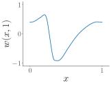
(d)

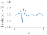
(e)

Figure 5: Example of training data and test prediction and pointwise errors for the Burger’s equation (49).

4.3.2 Darcy flow

Consider the two-dimensional Darcy flow problem (3). Recall that in this example, we are interested in learning the mapping from the permeability field $u$ to the solution $v$ and the source term $w$ is assumed to be fixed, hence $\mathcal{D}\equiv\Omega=(0,1)^{2}$ and ${\mathcal{G}}^{\dagger}:u\mapsto v$. The coefficient $u$ is sampled by setting $u\sim\log\circ h_{\sharp}\mu$ where $\mu=\mathcal{GP}(0,(-\Delta+9I)^{-2})$ is a GP and $h$ is binary function mapping positive inputs to $12$ and negative inputs to $3$. The resulting permeability/diffusion coefficient $e^{u}$ is therefore piecewise constant. As in [47], we use a discretized grid of resolution $29\times 29$, with the data generated by the MATLAB PDE Toolbox. We use 1000 points for training and 200 points for testing. Figure 3 shows an example of training input and output of the map $\mathcal{G}^{\dagger}$, and an example of predictions along with pointwise error at the test stage.

4.3.3 Advection equations (I and II)

Consider the one-dimensional advection equation:

(50) $$\frac{\partial w}{\partial t}+\frac{\partial w}{\partial x} =0 x\in(0,1),t\in(0,1]$$

$$w(x,0) =u(x) x\in(0,1)$$

with $\mathcal{D}=(0,1)$ and periodic boundary conditions. Similar to the example for Burgers’ equation, we learn the mapping from the initial condition $u$ to $v=w(\cdot,0.5)$, the solution at $t=0.5$, i.e., ${\mathcal{G}}^{\dagger}:w(\cdot,0)\mapsto w(\cdot,0.5)$.

This problem was considered in [47, 19] with different distributions $\mu$ for the initial condition. We will show in the following section how these different distributions lead to different performances. In [47], henceforth referred to as Advection I, the initial condition is a square wave centered at $x=c$ of width $b$ and height $h$:

(51) $$u(x)=h\mathbb{1}_{\{c-\frac{b}{2},c+\frac{b}{2}\}},$$

where the parameters $(c,b,h)\sim\mathcal{U}([0.3,0.7]\times[0.3,06]\times[1,2])$. In [19], henceforth referred to as Advection II, the initial condition is

(52) $$u=-1+2\mathbb{1}\{\tilde{u}_{0}\geq 0\}$$

where $\tilde{u}_{0}\sim\mathcal{GP}(0,(-\Delta+3^{2}I)^{-2})$.

For Advection I, the spatial grid was of resolution 40, and we used 1000 instances for training and 200 instances for testing. For Advection II, the resolution was of 200 and we used 20000 training and test instances, following [19].

Figures 6 and 7 show an example of training input and output for Advection the I and II problems, respectively. Observe that the functional samples from the distribution in Advection I will have exactly two discontinuities almost surely, but the samples for Advection II can have many more jumps. We observe that prediction is challenging around discontinuities, hence Advection II is a significantly harder problem (across all benchmarked methods) than Advection I. Figures 6 and 7 also show an instance of a test sample, along with a prediction and the pointwise errors.

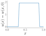
(a)

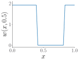
(b)

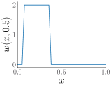
(c)

(d)

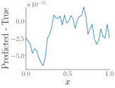
(e)

Figure 6: Example of training data and test prediction and pointwise errors for the Advection problem (50)-I.

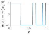
(a)

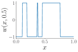
(b)

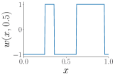
(c)

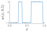
(d)

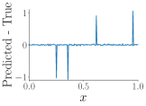
(e)

Figure 7: Example of training data and test prediction and pointwise errors for the Advection problem (50)-II.

4.3.4 Helmholtz’s equation

For a given frequency $\omega$ and wavespeed field $u:\mathcal{D}\to\mathbb{R}$, with $\mathcal{D}=(0,1)^{2}$, the excitation field $v:\mathcal{D}\to\mathbb{R}$ solves

(53) $$\left(-\Delta-\frac{\omega^{2}}{u^{2}(x)}\right)v=0,\quad x\in(0,1)^{2}$$

$$\frac{\partial v}{\partial n}=0,\quad x\in\{0,1\}\times[0,1]\cup[0,1]\times\{0\}\quad\text{and}\quad\frac{\partial v}{\partial n}=v_{N},\quad x\in[0,1]\times\{1\}$$

In the results that follow, we take $\omega=10^{3}$, $v_{N}=\mathbb{1}_{\{0.35\leq x\leq 0.65\}}$, and we aim to learn the map ${\mathcal{G}}:u\mapsto v$, i.e., the mapping from the wavespeed field to the excitation field. The distribution $\mu$ is specified as the law of $u(x)=20+\tanh(\tilde{u}(x))$, where $\tilde{u}$ is drawn from the GP, $\mathcal{GP}(0,(-\Delta+3^{2}I)^{-2})$. The training and test data were generated by solving (53) with a Finite Element Method on a discretization of size $100\times 100$ of the unit square. Figure 8 shows an example of training input and output, a test prediction, and pointwise errors.

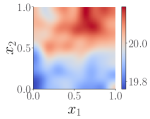
(a)

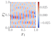
(b)

(c)

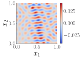
(d)

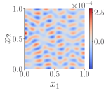
(e)

Figure 8: Example of training data and test prediction and pointwise errors for the Helmholtz problem (53).

4.3.5 Structural mechanics

We let $\Omega=[0,1]$ $D=[0,1]^{2}$, the equation that governs the displacement vector $w$ in an elastic solid undergoing infinitesimal deformations is

(54) $$\nabla\cdot\sigma=0\quad\text{in }(0,1)^{2},\qquad w=\bar{w},\quad\text{on }\Gamma_{w},\qquad\nabla\cdot n=u\quad\text{on }\Gamma_{u},$$

where the boundary $\partial D$ is split in $[0,1]\times{1}=\Gamma_{t}$ (the part of the boundary subject to stress) and its complement $\Gamma_{u}$.

The goal is to learn the operator that maps the one-dimensional load $u$ on $\Gamma_{u}$ to the two-dimensional von Mises stress field $v$ on $\Omega$, i.e., ${\mathcal{G}}:u\mapsto v$. Here the distribution $\mu$ is $\mathcal{GP}(100,400^{2}(-\Delta+3^{2}I)^{-1})$, with $\Delta$ being the Laplacian subject to homogeneous Neumann boundary conditions on the space of zero-mean functions. The function $v$ was obtained by a finite element code, see [19] for implementation details and the constitutive model used. Figure 9 shows an example of training input and outputs, a test prediction, and pointwise errors.

(a)

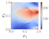
(b)

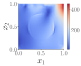
(c)

(d)

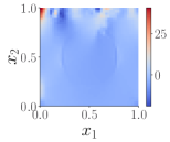
(e)

Figure 9: Example of training data and test prediction and pointwise errors for the Structural Mechanics problem (54).

4.3.6 Navier-Stokes equations

Consider the vorticity-stream $(\omega,\psi)$ formulation of the incompressible Navier-Stokes equations:

(55) $$\frac{\partial\omega}{\partial t}+(c\cdot\nabla)\omega-\nu\Delta\omega =u,\quad\omega =-\Delta\psi,\quad\int_{D}\psi =0,\quad c =\left(\frac{\partial\psi}{\partial x_{2}},-\frac{\partial\psi}{\partial x_{1}}\right)$$

where $\mathcal{D}=[0,2\pi]^{2}$, periodic boundary conditions are considered and the initial condition $w(\cdot,0)$ is fixed. Here we are interested in the mapping from the forcing term $u$ to $v=\omega(\cdot,T)$, the vorticity field at a given time $t=T$, i.e., ${\mathcal{G}}^{\dagger}:u\mapsto\omega(\cdot,T)$.

The distribution $\mu$ is $\mathcal{GP}(0,(-\Delta+3^{2}I)^{-4})$. The viscosity $\nu$ is fixed and equal to $0.025$, and the equation is solved on a $64\times 64$ grid with a pseudo-spectral method and Crank-Nicholson time integration; see [19] for further implementation details. Figure 10 shows an example of input and output in the test set, along with an example of test prediction and pointwise errors.

(a)

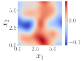
(b)

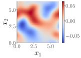
(c)

(d)

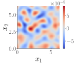
(e)

Figure 10: Example of training data and test prediction and pointwise errors for the Navier-Stokes problem (55).

4.4 Results and discussion

Below we discuss our main findings in benchmarking our kernel method against state-of-the-art NN based techniques

4.4.1 Performance against NNs

Table 3 summarizes the $L^{2}$ relative test error of our vanilla implementation of the kernel method along with those of DeepONet, FNO, PCA-Net, and PARA-Net. We observed that our vanilla kernel method was reliable in terms of accuracy across all examples. In particular, observe that between the Matérn or rational quadratic kernel, we always managed to get close to the other methods, see for example the results for the Burgers’ equation or Darcy problem, and even outperform them in several examples such as Navier-Stokes and Helmholtz. Overall we observed that the performance of the kernel method is stable across all examples suggesting that our method is reliable and provides a good baseline for a large class of problems. Moreover, we did not observe a significant difference in performance in terms of the choice of the particular kernel family once the hyper-parameters were tuned. This indicates that a large class of kernels are effective for these problems. Furthermore, we found the hyper-parameter tuning to be robust, i.e., results were consistent in a reasonable range of parameters such as length scales.

In the high data regime, we found the vanilla kernel method to be the most accurate, although this comes with a greater cost, as seen in Figure 11. However, the kernel method appears to provide the highest accuracy for its level of complexity as the accuracy of NNs typically stagnates or even decreases after a certain level of complexity; see the Navier-Stokes and Helmholtz panels of Figure 11 where most of the NN methods seem to plateau after a certain complexity level.

We also observed that the linear model did not provide the best accuracy as it quickly saturated in performance. Nonetheless, it provided surprisingly good accuracy at low levels of complexity: for example, in the case of Navier-Stokes, the linear kernel provided the best accuracy below $10^{6}$ FLOPS of complexity. This indicates that while simple, the linear model can be a valuable low-complexity model. Another notable example is the Advection equation (both I and II), where the operator $\mathcal{G}^{\dagger}$ is linear. In this case, the linear kernel had the best accuracy and the best complexity-accuracy tradeoff. We note, however, that while the linear model was close to machine precision on Advection I (error on the order $10^{-13}\%$), its performance was significantly worse on Advection II (error on the order of $10\%$). Moreover, the gap between the linear kernel and all other models was significantly smaller for Advection I; we conjecture this difference in performance is likely due to the setup of these problems.

Finally, we note that the most challenging problem for our kernel method was the Structural Mechanics example. In this case, the vanilla kernel method has higher complexity but did not beat the NNs. In fact, the NNs seem to be able to reduce complexity without loss of accuracy compared to our method.

	Low-data regime			High-data regime
	Burger’s	Darcy problem	Advection I	Advection II	Hemholtz	Structural Mechanics	Navier Stokes
DeepONet	2.15%	2.91%	0.66%	15.24%	5.88%	5.20%	3.63%
POD-DeepONet	1.94%	2.32%	0.04%	n/a	n/a	n/a	n/a
FNO	1.93%	2.41%	0.22%	13.49%	1.86%	4.76%	0.26%
PCA-Net	n/a	n/a	n/a	12.53%	2.13%	4.67%	2.65%
PARA-Net	n/a	n/a	n/a	16.64%	12.54%	4.55%	4.09%
Linear	36.24%	6.74%	$2.15\times 10^{-13}\%$	11.28%	10.59%	27.11%	5.41%
Best of Matérn/RQ	2.15%	2.75%	$2.75\times 10^{-3}\%$	11.44%	1.00%	5.18%	0.12%

Table 3: Summary of numerical results: we report the $L^{2}$ relative test error of our numerical experiments and compare the kernel approach with variations of DeepONet , FNO, PCA-Net and PARA-Net. We considered two choices of the kernel $S$, the rational quadratic and the Matérn, but we observed little difference between the two.

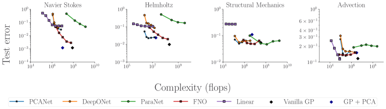
Figure 11: Accuracy complexity tradeoff achieved in the problems in [19]. Data for NNs was obtained from the aforementioned article. Linear model refers to the linear kernel, vanilla GP is our implementation with the nonlinear kernels and minimal preprocessing, GP+PCA corresponds to preprocessing through PCA both the input and the output to reduce complexity.

4.4.2 Effect of preconditioners

Table 4 compares the performance of our method with the Matérn kernel family using various preconditioning steps. Overall we observed that both PCA and Cholesky preconditioning improved the performance of our vanilla kernel method.

The Cholesky preconditioning generally offers the greatest improvement. However, we observed that getting the best results from the Cholesky approach required careful tuning of the parameters of the kernels $K$ and $Q$ which we did using cross-validation. While tuning the parameters does not increase the inference complexity, it does increase the training complexity.

On the other hand, the PCA approach was more robust to changes in hyperparameters, i.e., the number of PCA components following Section 4.1.2. We observed that applying PCA on the input and output reduces complexity and has varying levels of effectiveness in providing a better cost-accuracy tradeoff. For example, for Navier-Stokes, it greatly reduced the complexity without affecting accuracy. But for the Helmholtz and Advection equations, PCA reduced the accuracy while remaining competitive with NN models. For structural mechanics, however, PCA significantly reduced accuracy and was worse than other models. We hypothesize that the loss in accuracy can be related to the decay of the eigenvalues of the PCA matrix in that example.

	Advection II	Burger’s	Darcy problem
No preprocessing	14.37%	3.04%	4.47%
PCA	14.50%	2.41%	2.89%
Cholesky	11.44%	2.15%	2.75%

Table 4: Comparison between Cholesky preconditioning and PCA dimensionality reduction on three examples for our vanilla kernel implementation with the Matérn kernel.

5 Conclusions

In this work we presented a kernel/GP framework for the learning of operators between function spaces. We presented an abstract formulation of our kernel framework along with convergence proofs and error bounds in certain asymptotic limits. Numerical experiments and benchmarking against popular NN based algorithms revealed that our vanilla implementation of the kernel approach is competitive and either matches the performance of NN methods or beats them in several benchmarks. Due to simplicity of implementation, flexibility, and the empirical results, we suggest that the proposed kernel methods are a good benchmark for future, perhaps more sophisticated, algorithms. Furthermore, these methods can be used to guide practitioners in the design of new and challenging benchmarks (e.g, identify problems where vanilla kernel methods do not perform well). Numerous directions of future research exist. In the theoretical direction it is interesting to remove the stringent 3.2 and we anticipate this to require a particular selection of the kernel employed to obtain the map $\bar{f}$. Moreover, obtaining error bounds for more general measurement functionals beyond pointwise evaluations would be interesting. One could also adapt our framework to non-vanilla kernel methods such as random features or inducing point methods to provide a low-complexity alternative to NNs in the large-data regime. Finally, since the proposed approach is essentially a generalization of GP Regression to the infinite-dimensional setting, we anticipate that some of the hierarchical techniques of [58, 68, 70] could be extended to this setting and provide a better cost-accuracy trade-off than current methods.

Acknowledgments

MD, PB, and HO acknowledge support by the Air Force Office of Scientific Research under MURI award number FA9550-20-1-0358 (Machine Learning and Physics-Based Modeling and Simulation). BH acknowledges support by the National Science Foundation grant number NSF-DMS-2208535 (Machine Learning for Bayesian Inverse Problems). HO also acknowedges support by the Department of Energy under award number DE-SC0023163 (SEA-CROGS: Scalable, Efficient and Accelerated Causal Reasoning Operators, Graphs and Spikes for Earth and Embedded Systems). We thank F. Schäfer for comments and references.

Appendix A Review of operator valued kernels and GPs

We review the theory of operator valued kernels and GPs [60] as these are utilized throughout the article. Operator-valued kernels were introduced in [36] as a generalization of vector-valued kernels [3].

A.1 Operator valued kernels

Let $\mathcal{U}$ and $\mathcal{V}$ be separable Hilbert spaces endowed with the inner products $\big{\langle}\cdot,\cdot\big{\rangle}_{\mathcal{U}}$ and $\big{\langle}\cdot,\cdot\big{\rangle}_{\mathcal{V}}$. Write ${\mathcal{L}}(\mathcal{V})$ for the set of bounded linear operators mapping $\mathcal{V}$ to $\mathcal{V}$.

Definition A.1.

We call $G\,:\,\mathcal{U}\times\mathcal{U}\rightarrow{\mathcal{L}}(\mathcal{V})$ an operator-valued kernel if

1. $G$ is Hermitian, i.e. $G(u,u^{\prime})=G(u^{\prime},u)^{T}$ for all $u,u^{\prime}\in\mathcal{U}\,$, writing $A^{T}$ for the adjoint of the operator $A$ with respect to $\big{\langle}\cdot,\cdot\big{\rangle}_{\mathcal{V}}$.

2. $G$ is non-negative, i.e., for all $m\in\mathbb{N}$ and any set of points $(u_{i},v_{i})_{i=1}^{m}\subset\mathcal{U}\times\mathcal{V}$ it holds that $\sum_{i,j=1}^{m}\big{\langle}v_{i},G(u_{i},u_{j})v_{j}\big{\rangle}_{\mathcal{V}}\geq 0.$

We call $G$ non-degenerate if $\sum_{i,j=1}^{m}\big{\langle}v_{i},G(u_{i},u_{j})v_{j}\big{\rangle}_{\mathcal{V}}=0$ implies $v_{i}=0$ for all $i$ whenever $u_{i}\not=u_{j}$ for $i\not=j$.

A.2 RKHSs

Each non-degenerate, locally bounded and separately continuous operator-valued kernel $G$ is in one to one correspondence with an RKHS ${\mathcal{H}}$ of continuous operators ${\mathcal{G}}\,:\,\mathcal{U}\rightarrow\mathcal{V}$ obtained as the closure of the linear span of the maps $z\mapsto G(z,u)v$ with respect to the inner product identified by the reproducing property

(56) $$\big{\langle}g,G(\cdot,u)v\big{\rangle}_{\mathcal{H}}=\big{\langle}g(u),v\big{\rangle}_{\mathcal{V}}$$

A.3 Feature maps

Let ${\mathcal{F}}$ be a separable Hilbert space (with inner product $\big{\langle}\cdot,\cdot\big{\rangle}_{\mathcal{F}}$ and norm $\|\cdot\|_{\mathcal{F}}$) and let $\psi\,:\,\mathcal{U}\rightarrow{\mathcal{L}}(\mathcal{V},{\mathcal{F}})$ be a continuous function mapping $\mathcal{U}$ to the space of bounded linear operators from $\mathcal{V}$ to ${\mathcal{F}}$.

Definition A.2.

We say that ${\mathcal{F}}$ and $\psi\,:\,\mathcal{U}\rightarrow{\mathcal{L}}(\mathcal{V},{\mathcal{F}})$ are a feature space and a feature map for the kernel $G$ if, for all $(u,u^{\prime},v,v^{\prime})\in\mathcal{U}^{2}\times\mathcal{V}^{2}$,

$$\big{\langle}v,G(u,u^{\prime})v^{\prime}\big{\rangle}=\big{\langle}\psi(u)v,\psi(u^{\prime})v^{\prime}\big{\rangle}_{\mathcal{F}}\,.$$

Write $\psi^{T}(u)$, for the adjoint of $\psi(u)$ defined as the linear function mapping ${\mathcal{F}}$ to $\mathcal{V}$ satisfying

$$\big{\langle}\psi(u)v,\alpha\big{\rangle}_{\mathcal{F}}=\big{\langle}v,\psi^{T}(u)\alpha\big{\rangle}_{\mathcal{V}}$$

for $u,v,\alpha\in\mathcal{U}\times\mathcal{V}\times{\mathcal{F}}$. Note that $\psi^{T}\,:\,\mathcal{U}\rightarrow{\mathcal{L}}({\mathcal{F}},\mathcal{V})$ is therefore a function mapping $\mathcal{U}$ to the space of bounded linear functions from ${\mathcal{F}}$ to $\mathcal{V}$. Writing $\alpha^{T}\alpha^{\prime}:=\big{\langle}\alpha,\alpha^{\prime}\big{\rangle}_{\mathcal{F}}$ for the inner product in ${\mathcal{F}}$ we can ease our notations by writing

(57) $$G(u,u^{\prime})=\psi^{T}(u)\psi(u^{\prime})\,$$

which is consistent with the finite-dimensional setting and $v^{T}G(u,u^{\prime})v^{\prime}=(\psi(u)v)^{T}(\psi(u^{\prime})v^{\prime})$ (writing $v^{T}v^{\prime}$ for the inner product in $\mathcal{V}$). For $\alpha\in{\mathcal{F}}$ write $\psi^{T}\alpha$ for the function $\mathcal{U}\rightarrow\mathcal{V}$ mapping $u\in\mathcal{U}$ to the element $v\in\mathcal{V}$ such that

$$\big{\langle}v^{\prime},v\big{\rangle}_{\mathcal{V}}=\big{\langle}v^{\prime},\psi^{T}(u)\alpha\big{\rangle}_{\mathcal{V}}=\big{\langle}\psi(u)v^{\prime},\alpha\big{\rangle}_{\mathcal{F}}\text{ for all }v^{\prime}\in\mathcal{V}\,.$$

We can, without loss of generality, restrict ${\mathcal{F}}$ to be the range of $(u,v)\rightarrow\psi(u)v$ so that the RKHS ${\mathcal{H}}$ defined by $G$ is the closure of the pre-Hilbert space spanned by $\psi^{T}\alpha$ for $\alpha\in{\mathcal{F}}$. Note that the reproducing property (56) implies that for $\alpha\in{\mathcal{F}}$

$$\big{\langle}\psi^{T}(\cdot)\alpha,\psi^{T}(\cdot)\psi(u)v\big{\rangle}_{\mathcal{H}}=\big{\langle}\psi^{T}(u)\alpha,v\big{\rangle}_{\mathcal{V}}=\big{\langle}\alpha,\psi(u)v\big{\rangle}_{\mathcal{F}}$$

for all $u,v\in\mathcal{U}\times\mathcal{V}$, which leads to the following theorem.

Theorem A.3.

The RKHS ${\mathcal{H}}$ defined by the kernel (57) is the linear span of $\psi^{T}\alpha$ over $\alpha\in{\mathcal{F}}$ such that $\|\alpha\|_{\mathcal{F}}<\infty$. Furthermore, $\big{\langle}\psi^{T}(\cdot)\alpha,\psi^{T}(\cdot)\alpha^{\prime}\big{\rangle}_{\mathcal{H}}=\big{\langle}\alpha,\alpha^{\prime}\big{\rangle}_{\mathcal{F}}$ and

$$\|\psi^{T}(\cdot)\alpha\|^{2}_{\mathcal{H}}=\|\alpha\|^{2}_{\mathcal{F}}\text{ for }\alpha,\alpha^{\prime}\in{\mathcal{F}}\,.$$

A.4 Interpolation

Let us consider the interpolation problem in operator valued RKHSs.

Problem 2.

Let ${\mathcal{G}}^{\dagger}$ be an unknown continuous operator mapping $\mathcal{U}$ to $\mathcal{V}$. Given the information ${\mathcal{G}}^{\dagger}({\bf{u}})={\bf{v}}$ with the data $({\bf{u}},{\bf{v}})\in\mathcal{U}^{N}\times\mathcal{V}^{N}$, approximate ${\mathcal{G}}^{\dagger}$.

Using the relative error in $\|\cdot\|_{{\mathcal{H}}}$-norm as a loss, the minimax optimal recovery solution of 2 is, by [61, Thm. 12.4,12.5], given by

(58) $$\begin{cases}\text{Minimize }&\|{\mathcal{G}}\|_{{\mathcal{H}}}^{2}\\ \text{subject to }&{\mathcal{G}}({\bf{u}})={\bf{v}}\end{cases}$$

The minimizer is then of the form ${\mathcal{G}}(\cdot)=\sum_{j=1}^{N}G(\cdot,u_{j})w_{j}\,,$ where the coefficients $w_{j}\in\mathcal{V}$ are identified by solving the system of linear equations $\sum_{j=1}^{N}G(u_{i},u_{j})w_{j}=v_{i}\text{ for all }i\in\{1,\ldots,N\}\,.$ Using our compressed notation we can rewrite this equation as $G({\bf{u}},{\bf{u}}){\bf w}={\bf{v}}$ where ${\bf w}=(w_{1},\ldots,w_{N}),\,{\bf{v}}=(v_{1},\ldots,v_{N})\in\mathcal{V}^{N}$ and $G({\bf{u}},{\bf{u}})$ is the $N\times N$ block-operator matrix with entries $G(u_{i},u_{j})$. Therefore, writing $G(\cdot,{\bf{u}})$ for the vector $(G(\cdot,u_{1}),\ldots,G(\cdot,u_{N}))\in{\mathcal{H}}^{N}$, the optimal recovery interpolant is given by

(59) $$\bar{{\mathcal{G}}}(\cdot)=G(\cdot,{\bf{u}})G({\bf{u}},{\bf{u}})^{-1}{\bf{v}}\,,$$

which implies that the value of (58) at the minimum is

(60) $$\|\bar{{\mathcal{G}}}\|_{\mathcal{H}}^{2}={\bf{v}}^{T}G({\bf{u}},{\bf{u}})^{-1}{\bf{v}}\,,$$

where $G({\bf{u}},{\bf{u}})^{-1}$ is the inverse of $G({\bf{u}},{\bf{u}})$, whose existence is implied by the non-degeneracy of $G$ combined with $u_{i}\not=u_{j}$ for $i\not=j$.

A.5 Ridge regression

Let $\gamma>0$. A ridge regression (approximate) solution to Problem 2 can be found as the minimizer of

(61) $$\inf_{{\mathcal{G}}\in{\mathcal{H}}}\lambda\,\|{\mathcal{G}}\|_{\mathcal{H}}^{2}+\gamma^{-1}\sum_{i=1}^{N}\|v_{i}-{\mathcal{G}}(u_{i})\|_{\mathcal{V}}^{2}\,.$$

This minimizer is given by the formula

(62) $$\bar{{\mathcal{G}}}(u)=G(u,{\bf{u}})\big{(}G({\bf{u}},{\bf{u}})+\gamma I\big{)}^{-1}{\bf{v}}\,,$$

writing $I$ for the identity matrix. We can further compute directly

$$\|\bar{{\mathcal{G}}}\|_{\mathcal{H}}^{2}={\bf{v}}^{T}\big{(}G({\bf{u}},{\bf{u}})+\gamma I\big{)}^{-1}{\bf{v}}\,.$$

A.6 Operator-valued GPs

The following definition of operator-valued Gaussian processes is a natural extension of scalar-valued Gaussian fields [61].

Definition A.4.

[60, Def. 5.1] Let $G\,:\,\mathcal{U}\times\mathcal{U}\rightarrow{\mathcal{L}}(\mathcal{V})$ be an operator-valued kernel. Let $m$ be a function mapping $\mathcal{U}$ to $\mathcal{V}$. We call $\xi\,:\,\mathcal{U}\rightarrow{\mathcal{L}}(\mathcal{V},{\bf H})$ an operator-valued GP if $\xi$ is a function mapping $u\in\mathcal{U}$ to $\xi(u)\in{\mathcal{L}}(\mathcal{V},{\bf H})$ where ${\bf H}$ is a Gaussian space and ${\mathcal{L}}(\mathcal{V},{\bf H})$ is the space of bounded linear operators from $\mathcal{V}$ to ${\bf H}$. Abusing notations we write $\big{\langle}\xi(u),v\big{\rangle}_{\mathcal{V}}$ for $\xi(u)v$. We say that $\xi$ has mean $m$ and covariance kernel $G$ and write $\xi\sim{\mathcal{N}}(m,G)$ if $\big{\langle}\xi(u),v\big{\rangle}_{\mathcal{V}}\sim{\mathcal{N}}\big{(}m(u),v^{T}G(u,u)v\big{)}$ and

(63) $$\operatorname{Cov}\big{(}\big{\langle}\xi(u),v\big{\rangle}_{\mathcal{V}},\big{\langle}\xi(u^{\prime}),v^{\prime}\big{\rangle}_{\mathcal{V}}\big{)}=v^{T}G(u,u^{\prime})v^{\prime}\,.$$

We say that $\xi$ is centered if it is of zero mean.

If $G(u,u)$ is trace class ($\operatorname{Tr}[G(u,u)]<\infty$) then $\xi(u)$ defines a measure on $\mathcal{V}$, i.e. a $\mathcal{V}$-valued random variable .

Theorem A.5.

[60, Thm. 5.2] The law of an operator-valued GP is uniquely determined by its mean $m$ and covariance kernel $G$. Conversely given $m$ and $G$ there exists an operator-valued GP having mean $m$ and covariance kernel $G$. In particular if $G$ has feature space ${\mathcal{F}}$ and map $\psi$, the $e_{i}$ form an orthonormal basis of ${\mathcal{F}}$, and the $Z_{i}$ are i.i.d. ${\mathcal{N}}(0,1)$ random variables, then $\xi=m+\sum_{i}Z_{i}\psi^{T}e_{i}$ is an operator-valued GP with mean $m$ and covariance kernel $G$.

Theorem A.6.

[60, Thm. 5.3] Let $\xi$ be a centered operator-valued GP with covariance kernel $G\,:\,\mathcal{U}\times\mathcal{U}\rightarrow{\mathcal{L}}(\mathcal{V})$. Let ${\bf{u}},{\bf{v}}\in\mathcal{U}^{N}\times\mathcal{V}^{N}$. Let $Z=(Z_{1},\ldots,Z_{N})$ be a random Gaussian vector, independent from $\xi$, with i.i.d. ${\mathcal{N}}(0,\gamma I_{\mathcal{V}})$ entries ($\gamma\geq 0$ and $I_{\mathcal{V}}$ is the identity map on $\mathcal{V}$). Then $\xi$ conditioned on $\xi({\bf{u}})+Z$ is an operator-valued GP with mean

(64) $${\mathbb{E}}\big{[}\xi(u)\big{|}\xi({\bf{u}})+Z={\bf{v}}\big{]}=G(u,{\bf{u}})\big{(}G({\bf{u}},{\bf{u}})+\gamma I_{\mathcal{V}}\big{)}^{-1}{\bf{v}}=\eqref{eqajkjwdhjbdjehr}$$

and conditional covariance operator

(65) $$G^{\perp}(u,u^{\prime}):=G(u,u^{\prime})-G(u,{\bf{u}})\big{(}G({\bf{u}},{\bf{u}})+\gamma I_{\mathcal{V}}\big{)}^{-1}G({\bf{u}},u^{\prime})\,.$$

In particular, if $G$ is trace class, then

(66) $$\sigma^{2}(u):={\mathbb{E}}\Big{[}\big{\|}\xi(u)-{\mathbb{E}}[\xi(u)|\xi({\bf{u}})+Z={\bf{v}}]\big{\|}_{\mathcal{V}}^{2}\Big{|}\xi({\bf{u}})+Z={\bf{v}}\Big{]}=\operatorname{Tr}\big{[}G^{\perp}(u,u)\big{]}\,.$$

A.7 Deterministic error estimates for operator-valued regression

The following theorem shows that the standard deviation (66) provides deterministic a prior error bounds on the accuracy of the ridge regressor (64) to ${\mathcal{G}}^{\dagger}$ in Problem 2. Local error estimates such as (67) below are classical in the Kriging literature [77] where $\sigma^{2}(u)$ is known as the power function/kriging variance; see also [57][Thm. 5.1] for applications to PDEs.

Theorem A.7.

[60, Thm. 5.4] Let ${\mathcal{G}}^{\dagger}$ be the unknown function of Problem 2 and let ${\mathcal{G}}(u)=\eqref{eqlkwjldkjhjedkhe}=\eqref{eqajkjwdhjbdjehr}$ be its ridge regressor. Let ${\mathcal{H}}$ be the RKHS associated with $G$ and let ${\mathcal{H}}_{\gamma}$ be the RKHS associated with the kernel $G_{\gamma}:=G+\gamma I_{\mathcal{V}}$. It holds true that

(67) $$\big{\|}{\mathcal{G}}^{\dagger}(u)-{\mathcal{G}}(u)\big{\|}_{\mathcal{V}}\leq\sigma(u)\|{\mathcal{G}}^{\dagger}\|_{\mathcal{H}}$$

and

(68) $$\big{\|}{\mathcal{G}}^{\dagger}(u)-{\mathcal{G}}(u)\big{\|}_{\mathcal{V}}\leq\sqrt{\sigma^{2}(u)+\gamma\operatorname{dim}(\mathcal{V})}\|{\mathcal{G}}^{\dagger}\|_{{\mathcal{H}}_{\gamma}}\,,$$

where $\sigma(u)$ is the standard deviation (66).

Appendix B An alternative regularization of operator regression

For $\gamma>0$, the regularization implied by (27) is equivalent to adding noise on the $\varphi({\bf{v}})$ measurements. If one could observe ${\bf{v}}$ (and not just $\varphi({\bf{v}})$), then an alternative approach to regularizing the problem is to add noise to $\xi({\bf{u}})$. To describe this let $Z^{\prime}=(Z_{1}^{\prime},\ldots,Z_{N}^{\prime})$ be a random block-vector, independent from $\xi$, with i.i.d. entries $Z^{\prime}_{j}\sim{\mathcal{N}}(0,\gamma I_{\mathcal{V}})$ for $j=1,\dots,N$ (where $I_{\mathcal{V}}$ denotes the identity map on $\mathcal{V}$). Then the GP $\xi$ conditioned on $\xi({\bf{u}})={\bf{v}}+Z^{\prime}$ is a GP with conditional covariance kernel (65) and conditional mean $\tilde{{\mathcal{G}}}_{\gamma}$=(62) that is also the minimizer of (61). Observing that $\varphi(Z_{i}^{\prime})\sim{\mathcal{N}}(0,\gamma K(\varphi,\varphi))$ , we deduce that $\tilde{{\mathcal{G}}}_{\gamma}=\chi\circ\tilde{f}_{\gamma}\circ\phi$ where $\tilde{f}_{\gamma}$ minimizes

(69) $$\begin{cases}\text{Minimize }&\|f\|_{\Gamma}^{2}+\gamma^{-1}\sum_{i=1}^{N}(f(U_{i})-V_{i})^{T}K(\varphi,\varphi)^{-1}(f(U_{i})-V_{i})\,.\\ \text{Over }&f\in{\mathcal{H}}_{\Gamma}\,.\end{cases}$$

Furthermore, the distribution of $\xi$ conditioned on $\xi({\bf{u}})={\bf{v}}+Z^{\prime}$ is that of $\chi\circ\tilde{\zeta}^{\perp}\circ\phi$ where $\tilde{\zeta}^{\perp}\sim{\mathcal{N}}(\tilde{f}_{\gamma},\tilde{\Gamma}^{\perp})$ is the GP $\zeta$ conditioned on $\zeta({\bf{U}})={\bf{V}}+\varphi(Z^{\prime})$, whose mean is $\tilde{f}_{\gamma}$ and conditional covariance kernel is $\tilde{\Gamma}^{\perp}(U,U^{\prime})=\Gamma(U,U^{\prime})-\Gamma(U,{\bf{U}})(\Gamma({\bf{U}},{\bf{U}})+\gamma A)^{-1}\Gamma({\bf{U}},U^{\prime})$ where $A$ is a $N\times N$ block diagonal matrix with $K(\varphi,\varphi)$ as diagonal entries.

Appendix C Expressions for the kernels used in experiments

Below we collect the expressions for the kernels that were referred to in the article or utilized for our numerical experiments. These can be found in many standard textbooks on GPs such as [67].

C.1 The linear kernel

The linear kernel has the simple expression $K_{\text{linear}}(x,x^{\prime})=\big{\langle}x,x^{\prime}\big{\rangle}$ and may be defined on any inner product space. It has no hyper-parameters.

C.2 The rational quadratic kernel

The rational quadratic kernel has the expression $K(x,x^{\prime})=k_{\text{RQ}}(\|x-x^{\prime}\|)$ where

(70) $$k_{\text{RQ}}(r)=\bigg{(}1+\frac{r^{2}}{2l^{2}}\bigg{)}^{-\alpha}.$$

It has hyper-parameters $\alpha>0$ and $l$.

C.3 The Matérn parametric family

The Matérn kernel family is of the form $K(x,x^{\prime})=k(\|x-x^{\prime}\|$ where

(71) $$k_{\nu}(r)=\exp\bigg{(}-\frac{\sqrt{2\nu}r}{l}\bigg{)}\frac{\Gamma(p+1)}{\Gamma(2p+1)}\sum_{i=0}^{p}\frac{(p+1)!}{i!(p-i)!}\bigg{(}\frac{\sqrt{8\nu}r}{l}\bigg{)}^{p-i},$$

for $\nu=p+\frac{1}{2}$. This kernel has hyper-parameters $p\in\mathbb{Z}_{+}$ and $l>0$. In the limiting case where $\nu\to\infty$, the Matérn kernel, we obtain the Gaussian or squared exponential kernel:

(72) $$k_{\infty}(r)=\exp\bigg{(}-\frac{r^{2}}{2l^{2}}\bigg{)},$$

with hyper-parameter $l>0$.

References

- [1] B. O. Almroth, P. Stern, and F. A. Brogan, Automatic choice of global shape functions in structural analysis, Aiaa Journal, 16 (1978), pp. 525–528.
- [2] R. Altmann, P. Henning, and D. Peterseim, Numerical homogenization beyond scale separation, Acta Numerica, 30 (2021), pp. 1–86.
- [3] M. A. Alvarez, L. Rosasco, N. D. Lawrence, et al., Kernels for vector-valued functions: A review, Foundations and Trends® in Machine Learning, 4 (2012), pp. 195–266.
- [4] D. Amsallem and C. Farhat, Interpolation method for adapting reduced-order models and application to aeroelasticity, AIAA journal, 46 (2008), pp. 1803–1813.
- [5] R. Arcangéli, M. C. López de Silanes, and J. J. Torrens, An extension of a bound for functions in sobolev spaces, with applications to (m, s)-spline interpolation and smoothing, Numerische Mathematik, 107 (2007), pp. 181–211.
- [6] L. S. Bastos and A. O’hagan, Diagnostics for gaussian process emulators, Technometrics, 51 (2009), pp. 425–438.
- [7] J. Beck, R. Tempone, F. Nobile, and L. Tamellini, On the optimal polynomial approximation of stochastic pdes by galerkin and collocation methods, Mathematical Models and Methods in Applied Sciences, 22 (2012), p. 1250023.
- [8] M. P. Bendsoe and O. Sigmund, Topology optimization: theory, methods, and applications, Springer Science & Business Media, 2003.
- [9] K. Bhattacharya, B. Hosseini, N. B. Kovachki, and A. M. Stuart, Model Reduction And Neural Networks For Parametric PDEs, The SMAI Journal of computational mathematics, 7 (2021), pp. 121–157.
- [10] G. Boncoraglio and C. Farhat, Active manifold and model-order reduction to accelerate multidisciplinary analysis and optimization, AIAA Journal, 59 (2021), pp. 4739–4753.
- [11] N. Boullé and A. Townsend, Learning elliptic partial differential equations with randomized linear algebra, Foundations of Computational Mathematics, (2022), pp. 1–31.
- [12] T. Chen and H. Chen, Approximation capability to functions of several variables, nonlinear functionals, and operators by radial basis function neural networks, IEEE Transactions on Neural Networks, 6 (1995), pp. 904–910.
- [13] T. Chen and H. Chen, Universal approximation to nonlinear operators by neural networks with arbitrary activation functions and its application to dynamical systems, IEEE Transactions on Neural Networks, 6 (1995), pp. 911–917.
- [14] Y. Chen, B. Hosseini, H. Owhadi, and A. M. Stuart, Solving and learning nonlinear pdes with gaussian processes, 2021.
- [15] Y. Chen, H. Owhadi, and A. Stuart, Consistency of empirical bayes and kernel flow for hierarchical parameter estimation, Mathematics of Computation, 90 (2021), pp. 2527–2578.
- [16] A. Chkifa, A. Cohen, R. DeVore, and C. Schwab, Sparse adaptive taylor approximation algorithms for parametric and stochastic elliptic PDEs, ESAIM: Mathematical Modelling and Numerical Analysis, 47 (2012), pp. 253–280.
- [17] A. Chkifa, A. Cohen, and C. Schwab, High-dimensional adaptive sparse polynomial interpolation and applications to parametric pdes, Foundations of Computational Mathematics, 14 (2014), pp. 601–633.
- [18] A. Cohen and R. DeVore, Approximation of high-dimensional parametric pdes, Acta Numerica, 24 (2015), pp. 1–159.
- [19] M. De Hoop, D. Z. Huang, E. Qian, and A. M. Stuart, The cost-accuracy trade-off in operator learning with neural networks, arXiv preprint arXiv:2203.13181, (2022).
- [20] B. Deng, Y. Shin, L. Lu, Z. Zhang, and G. E. Karniadakis, Approximation rates of deeponets for learning operators arising from advection–diffusion equations, Neural Networks, 153 (2022), pp. 411–426.
- [21] T. D. Economon, F. Palacios, S. R. Copeland, T. W. Lukaczyk, and J. J. Alonso, Su2: An open-source suite for multiphysics simulation and design, Aiaa Journal, 54 (2016), pp. 828–846.
- [22] Y. Fan, C. O. Bohorquez, and L. Ying, BCR-Net: A neural network based on the nonstandard wavelet form, Journal of Computational Physics, 384 (2019), pp. 1–15.
- [23] Y. Fan, J. Feliu-Faba, L. Lin, L. Ying, and L. Zepeda-Núnez, A multiscale neural network based on hierarchical nested bases, Research in the Mathematical Sciences, 6 (2019), pp. 1–28.
- [24] Y. Fan, L. Lin, L. Ying, and L. Zepeda-Núnez, A multiscale neural network based on hierarchical matrices, Multiscale Modeling & Simulation, 17 (2019), pp. 1189–1213.
- [25] M. Feischl and D. Peterseim, Sparse compression of expected solution operators, SIAM Journal on Numerical Analysis, 58 (2020), pp. 3144–3164.
- [26] F. Feyel and J.-L. Chaboche, Fe2 multiscale approach for modelling the elastoviscoplastic behaviour of long fibre sic/ti composite materials, Computer methods in applied mechanics and engineering, 183 (2000), pp. 309–330.
- [27] J. Fish, K. Shek, M. Pandheeradi, and M. S. Shephard, Computational plasticity for composite structures based on mathematical homogenization: Theory and practice, Computer methods in applied mechanics and engineering, 148 (1997), pp. 53–73.
- [28] R. G. Ghanem and P. D. Spanos, Stochastic finite elements: a spectral approach, Dover Publications, 2003.
- [29] C. R. Gin, D. E. Shea, S. L. Brunton, and J. N. Kutz, Deepgreen: deep learning of green’s functions for nonlinear boundary value problems, Scientific reports, 11 (2021), p. 21614.
- [30] M. D. Gunzburger, C. G. Webster, and G. Zhang, Stochastic finite element methods for partial differential equations with random input data, Acta Numerica, 23 (2014), pp. 521–650.
- [31] B. Hamzi, R. Maulik, and H. Owhadi, Simple, low-cost and accurate data-driven geophysical forecasting with learned kernels, Proceedings of the Royal Society A, 477 (2021), p. 20210326.
- [32] B. Hamzi and H. Owhadi, Learning dynamical systems from data: a simple cross-validation perspective, part i: parametric kernel flows, Physica D: Nonlinear Phenomena, 421 (2021), p. 132817.
- [33] J. Hesthaven and S. Ubbiali, Non-intrusive reduced order modeling of nonlinear problems using neural networks, Journal of Computational Physics, 363 (2018), pp. 55–78.
- [34] J. S. Hesthaven, G. Rozza, B. Stamm, et al., Certified reduced basis methods for parametrized partial differential equations, vol. 590, Springer, 2016.
- [35] D. Z. Huang, T. Schneider, and A. M. Stuart, Iterated kalman methodology for inverse problems, Journal of Computational Physics, 463 (2022), p. 111262.
- [36] H. Kadri, E. Duflos, P. Preux, S. Canu, A. Rakotomamonjy, and J. Audiffren, Operator-valued kernels for learning from functional response data, (2016).
- [37] M. C. Kennedy and A. O’Hagan, Bayesian calibration of computer models, Journal of the Royal Statistical Society: Series B (Statistical Methodology), 63 (2001), pp. 425–464.
- [38] Y. Khoo, J. Lu, and L. Ying, Solving parametric pde problems with artificial neural networks, European Journal of Applied Mathematics, 32 (2021), pp. 421–435.
- [39] Y. Khoo and L. Ying, Switchnet: a neural network model for forward and inverse scattering problems, SIAM Journal on Scientific Computing, 41 (2019), pp. A3182–A3201.
- [40] G. Kissas, J. H. Seidman, L. F. Guilhoto, V. M. Preciado, G. J. Pappas, and P. Perdikaris, Learning operators with coupled attention, Journal of Machine Learning Research, 23 (2022), pp. 1–63.
- [41] N. Kovachki, S. Lanthaler, and S. Mishra, On universal approximation and error bounds for fourier neural operators, The Journal of Machine Learning Research, 22 (2021), pp. 13237–13312.
- [42] N. Kovachki, B. Liu, X. Sun, H. Zhou, K. Bhattacharya, M. Ortiz, and A. Stuart, Multiscale modeling of materials: Computing, data science, uncertainty and goal-oriented optimization, Mechanics of Materials, 165 (2022), p. 104156.
- [43] K. Krischer, R. Rico-Martínez, I. Kevrekidis, H. Rotermund, G. Ertl, and J. Hudson, Model identification of a spatiotemporally varying catalytic reaction, AIChE Journal, 39 (1993), pp. 89–98.
- [44] F. Kröpfl, R. Maier, and D. Peterseim, Operator compression with deep neural networks, Advances in Continuous and Discrete Models, 2022 (2022), pp. 1–23.
- [45] Z. Li, N. Kovachki, K. Azizzadenesheli, B. Liu, K. Bhattacharya, A. Stuart, and A. Anandkumar, Fourier neural operator for parametric partial differential equations, 2020.
- [46] L. Lu, P. Jin, G. Pang, Z. Zhang, and G. E. Karniadakis, Learning nonlinear operators via DeepONet based on the universal approximation theorem of operators, Nature Machine Intelligence, 3 (2021), pp. 218–229.
- [47] L. Lu, X. Meng, S. Cai, Z. Mao, S. Goswami, Z. Zhang, and G. E. Karniadakis, A comprehensive and fair comparison of two neural operators (with practical extensions) based on fair data, Computer Methods in Applied Mechanics and Engineering, 393 (2022), p. 114778.
- [48] D. J. Lucia, P. S. Beran, and W. A. Silva, Reduced-order modeling: new approaches for computational physics, Progress in aerospace sciences, 40 (2004), pp. 51–117.
- [49] Y. Maday, A. T. Patera, and G. Turinici, A priori convergence theory for reduced-basis approximations of single-parameter elliptic partial differential equations, Journal of Scientific Computing, 17 (2002), pp. 437–446.
- [50] A. Målqvist and D. Peterseim, Localization of elliptic multiscale problems, Mathematics of Computation, 83 (2014), pp. 2583–2603.
- [51] J. Martin, L. C. Wilcox, C. Burstedde, and O. Ghattas, A stochastic newton mcmc method for large-scale statistical inverse problems with application to seismic inversion, SIAM Journal on Scientific Computing, 34 (2012), pp. A1460–A1487.
- [52] J. R. Martins and A. B. Lambe, Multidisciplinary design optimization: a survey of architectures, AIAA journal, 51 (2013), pp. 2049–2075.
- [53] N. Marzari, A. A. Mostofi, J. R. Yates, I. Souza, and D. Vanderbilt, Maximally localized wannier functions: Theory and applications, Reviews of Modern Physics, 84 (2012), p. 1419.
- [54] F. Nobile, R. Tempone, and C. G. Webster, An anisotropic sparse grid stochastic collocation method for partial differential equations with random input data, SIAM Journal on Numerical Analysis, 46 (2008), pp. 2411–2442.
- [55] F. Nobile, R. Tempone, and C. G. Webster, A sparse grid stochastic collocation method for partial differential equations with random input data, SIAM Journal on Numerical Analysis, 46 (2008), pp. 2309–2345.
- [56] A. K. Noor and J. M. Peters, Reduced basis technique for nonlinear analysis of structures, Aiaa journal, 18 (1980), pp. 455–462.
- [57] H. Owhadi, Bayesian numerical homogenization, Multiscale Modeling & Simulation, 13 (2015), pp. 812–828.
- [58] H. Owhadi, Multigrid with rough coefficients and multiresolution operator decomposition from hierarchical information games, Siam Review, 59 (2017), pp. 99–149.
- [59] H. Owhadi, Computational graph completion, Research in the Mathematical Sciences, 9 (2022), p. 27.
- [60] H. Owhadi, Do ideas have shape? idea registration as the continuous limit of artificial neural networks, Physica D: Nonlinear Phenomena, 444 (2023), p. 133592.
- [61] H. Owhadi and C. Scovel, Operator-Adapted Wavelets, Fast Solvers, and Numerical Homogenization: From a Game Theoretic Approach to Numerical Approximation and Algorithm Design, Cambridge Monographs on Applied and Computational Mathematics, Cambridge University Press, 2019.
- [62] H. Owhadi and G. R. Yoo, Kernel flows: from learning kernels from data into the abyss, Journal of Computational Physics, 389 (2019), pp. 22–47.
- [63] H. Owhadi and L. Zhang, Metric-based upscaling, Communications on Pure and Applied Mathematics: A Journal Issued by the Courant Institute of Mathematical Sciences, 60 (2007), pp. 675–723.
- [64] H. Owhadi and L. Zhang, Gamblets for opening the complexity-bottleneck of implicit schemes for hyperbolic and parabolic odes/pdes with rough coefficients, Journal of Computational Physics, 347 (2017), pp. 99–128.
- [65] F. Pedregosa, G. Varoquaux, A. Gramfort, V. Michel, B. Thirion, O. Grisel, M. Blondel, P. Prettenhofer, R. Weiss, V. Dubourg, J. Vanderplas, A. Passos, D. Cournapeau, M. Brucher, M. Perrot, and E. Duchesnay, Scikit-learn: Machine learning in Python, Journal of Machine Learning Research, 12 (2011), pp. 2825–2830.
- [66] S. Prasanth, Z. Haddad, J. Susiluoto, A. Braverman, H. Owhadi, B. Hamzi, S. Hristova-Veleva, and J. Turk, Kernel flows to infer the structure of convective storms from satellite passive microwave observations, in AGU Fall Meeting Abstracts, vol. 2021, 2021, pp. A55F–1445.
- [67] C. E. Rasmussen and C. K. I. Williams, Gaussian processes for machine learning., Adaptive computation and machine learning, MIT Press, 2006.
- [68] F. Schaäfer, M. Katzfuss, and H. Owhadi, Sparse Cholesky factorization by Kullback–Leibler minimization, SIAM Journal on scientific computing, 43 (2021), pp. A2019–A2046.
- [69] F. Schäfer and H. Owhadi, Sparse recovery of elliptic solvers from matrix-vector products, arXiv preprint arXiv:2110.05351, (2021).
- [70] F. Schäfer, T. J. Sullivan, and H. Owhadi, Compression, inversion, and approximate PCA of dense kernel matrices at near-linear computational complexity, Multiscale Modeling & Simulation, 19 (2021), pp. 688–730.
- [71] B. Schölkopf, R. Herbrich, and A. J. Smola, A generalized representer theorem, in Computational Learning Theory, D. Helmbold and B. Williamson, eds., Berlin, Heidelberg, 2001, Springer Berlin Heidelberg, pp. 416–426.
- [72] B. Sudret, S. Marelli, and J. Wiart, Surrogate models for uncertainty quantification: An overview, in 2017 11th European conference on antennas and propagation (EUCAP), IEEE, 2017, pp. 793–797.
- [73] J. Susiluoto, A. Braverman, P. Brodrick, B. Hamzi, M. Johnson, O. Lamminpaa, H. Owhadi, C. Scovel, J. Teixeira, and M. Turmon, Radiative transfer emulation for hyperspectral imaging retrievals with advanced kernel flows-based gaussian process emulation, in AGU Fall Meeting Abstracts, vol. 2021, 2021, pp. NG25A–0506.
- [74] S. Wang, H. Wang, and P. Perdikaris, Learning the solution operator of parametric partial differential equations with physics-informed deeponets, Science advances, 7 (2021), p. eabi8605.
- [75] S. Wang, H. Wang, and P. Perdikaris, Improved architectures and training algorithms for deep operator networks, Journal of Scientific Computing, 92 (2022), p. 35.
- [76] E. Weinan, Principles of multiscale modeling, Cambridge University Press, 2011.
- [77] Z.-m. Wu and R. Schaback, Local error estimates for radial basis function interpolation of scattered data, IMA journal of Numerical Analysis, 13 (1993), pp. 13–27.
- [78] D. Xiu, Numerical Methods for Stochastic Computations: A Spectral Method Approach, Princeton University Press, 2010.
- [79] D. Xiu and G. E. Karniadakis, The wiener–askey polynomial chaos for stochastic differential equations, SIAM journal on scientific computing, 24 (2002), pp. 619–644.
- [80] D. Xiu and J. Shen, Efficient stochastic galerkin methods for random diffusion equations, Journal of Computational Physics, 228 (2009), pp. 266–281.
- [81] Y. Zhu and N. Zabaras, Bayesian deep convolutional encoder–decoder networks for surrogate modeling and uncertainty quantification, Journal of Computational Physics, 366 (2018), pp. 415–447.