Graph-CoVis: GNN-based Multi-view Panorama Global Pose Estimation

Abstract

In this paper, we address the problem of wide-baseline camera pose estimation from a group of 360^∘ panoramas under upright-camera assumption. Recent work has demonstrated the merit of deep-learning for end-to-end direct relative pose regression in 360^∘ panorama pairs [11]. To exploit the benefits of multi-view logic in a learning-based framework, we introduce Graph-CoVis, which non-trivially extends CoVisPose [11] from relative two-view to global multi-view spherical camera pose estimation. Graph-CoVis is a novel Graph Neural Network based architecture that jointly learns the co-visible structure and global motion in an end-to-end and fully-supervised approach. Using the ZInD [4] dataset, which features real homes presenting wide-baselines, occlusion, and limited visual overlap, we show that our model performs competitively to state-of-the-art approaches.

1 Introduction

Camera pose estimation is a fundamental problem in computer vision and robotics. Whenever appropriate, constraints are used to both simplify the solution space and improve performance. One common constraint is that of planar camera motion. This is often the case when using sparsely captured $360^{\circ}$ panoramas for indoor applications. In our work, we address the multi-view pose estimation problem using $360^{\circ}$ panoramas with wide baselines within a large indoor space; we see this as a solution for an arbitrary number of visually connected panoramas.

CoVisPose [11] is a state-of-the-art end-to-end model for pairwise relative pose estimation in $360^{\circ}$ indoor panoramas. It models the visual overlap and correspondence constraints that are present between two panoramic views when parts of an indoor scene are commonly observed by both cameras. In particular, by exploiting the upright-camera assumption, co-visibility (visual overlap), correspondence, and layout geometry are framed as 1-D quantities estimated over the image columns. Using this formulation, visualized in Figure 1, CoVisPose demonstrates that learning such high-level geometric cues results in effective and robust representation for end-to-end pose estimation.

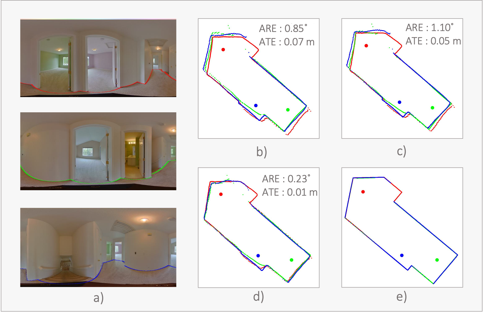
Figure 1: From three panoramas(a), Graph-CoVis(d) returns higher accuracy poses and visually consistent boundaries compared to two standard baselines based on relative pose estimation from CoVisPose[11] with greedy spanning tree(b) and pose graph optimization(c). Ground truth is shown in (e). ARE stands for absolute rotation error, and ATE stands for absolute translation error.

While CoVisPose achieves state-of-the-art results on wide-baseline relative pose estimation for pairs of 360^∘ panoramas, it does not provide an end-to-end solution for more than two panoramas. By comparison, we propose a more general end-to-end model for estimating the global poses for two or more panoramas.

Our end-to-end approach, called Graph-CoVis, extends the strengths of the pair-wise pose estimation model from CoVisPose [11] to a global multi-view pose estimation model. By using a Graph Neural Network (GNN) [22], Graph-CoVis retains the properties of the CoVisPose network that yield accurate pair-wise panorama pose estimates, while enabling it to generalize across multiple views and learn to regress consistent global poses.

Our technical contributions are as follow:

• Graph-CoVis is the first end-to-end architecture for multi-view panorama global pose estimation.

• Graph-CoVis is the first global pose estimation architecture that can effectively handle varying numbers of input panoramas.

• A message passing scheme that enables the GNN to leverage deep representations of dense visual overlap and boundary correspondence constraints, to better estimate global pose.

• Competitive performance on ZInD for global pose estimation in a group of panoramas.

2 Related work

Estimation of the motion between two cameras is commonly achieved through detection and matching of keypoints such as SIFT[15] across the two images, estimating the transformation matrix between the two views, and finally computing the relative translation and rotation between the two cameras[10]. Commonly, RANSAC[8] is used in the transformation estimation due to outliers in the matching stage.

Learned models have been proposed for each of the steps[27, 21, 12], combination of steps[7, 24], and the end-to-end pipeline[19, 3, 9, 18]. LIFT[27] is one of the first systems for a learned feature detector and descriptor, followed by more recent works such as SuperPoint[6], Keypoint matching is learned using a GNN architecture in Superglue [21] and a Transformer-based architecture in COTR[12]. D2-Net[7] is a learned joint detector and descriptor. Lofter[24] achieves detector-free matching across images by learning feature descriptors starting from a dense pixel-wise sampling and refining them for high quality fine-level matching. Differentiable RANSAC [2] enables robustness in the end-to-end training of the pipeline.

End-to-end methods regress a pose directly from two input images. DiffPoseNet[19] learns poses by modeling optical flow and pose estimation, replicating these key principles from geometric methods. Focusing on direction alone, DirectionNet[3] works even for challenging wide-baseline images. RegNet[9] learns both the feature representations and the Jacobian matrix used in the optimization of two-view pose. Using a translation and rotation equivariant convolutional neural network[18] improves the geometric information learned in the feature representations. A common theme in these recent end-to-end approaches is the explicit modeling of two-view geometry principles in the network. Similarly, we leverage the strong geometry priors that are inherent in panorama images.

GNNs have been used for multi-view pose estimation in different ways. Similar in spirit to our work, PoGO-Net[14] models multiple camera poses as nodes and uses a GNN with message passing scheme as an alternative to classical pose graph optimization. The method however requires an initialization method for the graph. In contrast, we do not require any explicit initialization. Our network densely connects each pose node to every other node and learns the dependencies between multiple views directly from the data. [20] is an end-to-end trained GNN model to learn matches across multiple views, where the GNN module is followed by a differentiable pose optimization module. In contrast to our model that learns and updates the underlying features of the pair-wise module, their model is focused on learning the optimal matching function between keypoints. Further, their model depends greatly on the accuracy of the pose optimizer to achieve good results.

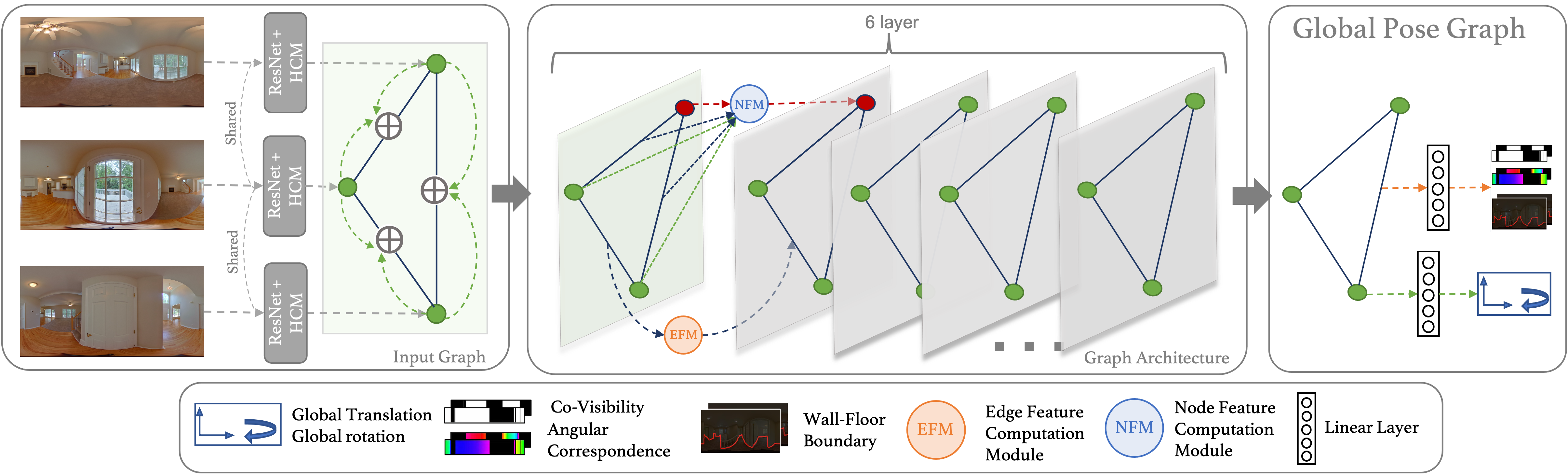
Figure 2: Graph-CoVis Architecture for a sample input of three panoramas. We initialize our graph’s node and edge representations using visual features as in [11], followed by six message passing layers to produce a Global Pose Graph. Nodes represent global poses and edges represent inter-frame geometric cues. The message passing process is: 1) the Edge Feature Computation Module (EFM) updates the edge features, 2) the Message Computation Module (MCM), where the target node’s features attend to the features of the source node and the adjoining edge, and 3) the Node Feature Computation Module (NFM) aggregates the incoming messages from all source nodes to update target node features. Finally, each node and edge are used to estimate global poses and pair-wise geometric cues, respectively.

Originally described for perspective images, some of the above methods have been applied on panorama images[17]. The 360-degree view in panoramas creates useful constraints and angular correspondences between columns of two images that have a visual overlap between them. CoVisPose[11] leverages these constraints along with geometric priors in the appearance of structures such as room layout boundaries to yield a highly accurate two-view pose estimation model. PSMNet[26] is a pose and layout estimator that predicts the joint layout from two panorama views and is able to regress the fine pose when initialized to approximations.

In our domain of multi-view panorama pose estimation notable recent works include estimating floor plans from extreme wide-baseline views (one panorama image per room)[23] and SALVe[13], a system for full floor plan reconstruction in sparsely sampled views. These works attempt to arrange all possible panoramas in the set, even those with little or no visual overlap, requiring alignment of semantic structures such as doors and walls. We address the problem of multi-view panorama pose estimation when panoramas have visual overlap between them, which is a key problem in full floor plan reconstruction.

3 Method

In this section, we describe our Graph-CoVis architecture in detail, as well as our training strategy. The overall architecture for a group of three panoramas is visualized in Figure 2. We start with briefly describing CoVisPose.

3.1 CoVisPose

CoVisPose[11] is an end-to-end method for pairwise pose estimation in wide baseline $360^{\circ}$ indoor panoramas. It uses geometric cues such as visible-boundary, co-visibility, and angular correspondence as auxiliary prediction outputs in order to effectively train a pose estimator. With features resulting from a ResNet backbone and a height compression module as input to the multi-layer transformer, it estimates the pose and geometric auxiliary outputs in separate branches.

The Graph-CoVis framework generalizes the pair-wise pose estimation model to multiple views in order to estimate the global pose instead of the relative pose. In comparison to CoVisPose our model is capable of understanding global information inside the graph and using GNNs, we demonstrate the extension to multiple views by defining the following representations.

3.2 Problem Representation

Given a group of input panoramas of size $N$, $\{\mathbf{I}_{i}\}_{i=1}^{N}\in\mathbb{R}^{3\times H\times W}$, without loss of generality we adopt $\mathbf{I}_{1}$ as the origin panorama, and estimate the remaining poses $\mathbf{P}_{2}$ to $\mathbf{P}_{n}$ in a shared coordinate system centered at the origin. We adopt the planar motion pose representation consisting of a translation vector $\mathbf{t}\in\mathbb{R}^{2}$ and a rotation matrix $R\in SO(2)$, i.e., the pose $\mathbf{P}_{i}\in SE(2)$. We represent the pose by 4 parameters, directly estimating the scaled translation vector $\mathbf{t}$, alongside the unit rotation vector $\mathbf{r}$.

3.3 Graph Representation

Defining the input directed graph as $\mathcal{G}=(\mathcal{V},\mathcal{E})$, we represent the set of panoramas with nodes $\mathcal{V}=\{v_{i}\}$, and model the inter-image relationships through the edge set $\mathcal{E}=\left\{e_{ij}\mid v_{i},v_{j}\in\mathcal{V}\right\}$.

3.3.1 Node and Edge Feature Initialization

Each node $v_{i}$ in the graph $\mathcal{G}$ is associated with the node features $\mathbf{x}_{i}^{l}$, where $l$ refers to the layer number. The input graph node features, $\mathbf{x}_{i}^{0}$, are initialized with the visual features $\psi_{i}$, extracted from panorama $\mathbf{I}_{i}$. We employ the feature extractor from[11], which consists of a ResNet50 backbone and a height compression module, followed by the addition of fixed positional encodings and six-layer transformer encoder. These structures are initialized from a pretrained CoVisPose model. Information about node identity is conveyed through learnable node embeddings. The node embeddings also indicate to the network which node is the origin of the global coordinate frame.

The edge features $\mathbf{e}_{ij}^{0}$ are initialized with the concatenation of $\psi_{i}$ and $\psi_{j}$. Prior to concatenation, we additionally add the pretrained segment embeddings to identify the node identity for later edge feature computations. These convey image membership to the following transformer encoder layer.

3.4 GraphCoVis Network Architecture

3.4.1 Message Passing

Our network’s representations are processed through six message passing layers to embed rich representations for pose regression. The message passing scheme is shown in Figure 3. We compute incoming messages for each node using the Message Computation Module (MCM). The MCM first updates the edge features using the Edge Feature Module (EFM), and subsequently uses these representations to construct messages which are aggregated in the Node Feature Computation Module (NFM), to update the node embeddings.

To update the edge features, the EFM consists of a single transformer encoder layer, the weights of which are initialized by the encoder layer weights from a pretrained CoVisPose model,

$$\mathbf{e}_{ij}^{l}=\theta_{E}^{l}(\mathbf{e}_{ij}^{l-1}),$$ (1)

where $\theta_{E}^{l}$ is the single-layer transformer encoder in the $l$th message passing layer, $\mathbf{e}_{ij}^{l-1}$ and $\mathbf{e}_{ij}^{l}$ are the edge features for edge $e_{ij}$ at the input and output of the EFM, respectively. After the edge features have been updated in Eq. 1, the MCM then computes incoming messages for each node prior to aggregation using a single-layer transformer decoder, $\theta_{M}^{l}$,

$$m_{j\rightarrow i}^{l}=\theta_{M}^{l}(\mathbf{x}_{i}^{l-1},\mathbf{x}_{j}^{l-1}\oplus\mathbf{e}_{ij}^{l}),$$ (2)

where $m_{j\rightarrow i}^{l}$ is the message from the source node $v_{j}$ to the target node $v_{i}$, and $\mathbf{x}_{j}^{l-1}\oplus\mathbf{e}_{ij}^{l}$ is the concatenation between the updated edge features $\mathbf{e}_{ij}^{l}$ and the existing node representation for the neighboring node $j$. In this way, the existing node representation attends to the inter-image information extracted along the edges, as well as the neighboring panoramas node representation.

We subsequently update the node embeddings by taking the mean over all incoming messages in the Node Feature Computation Module (NFM),

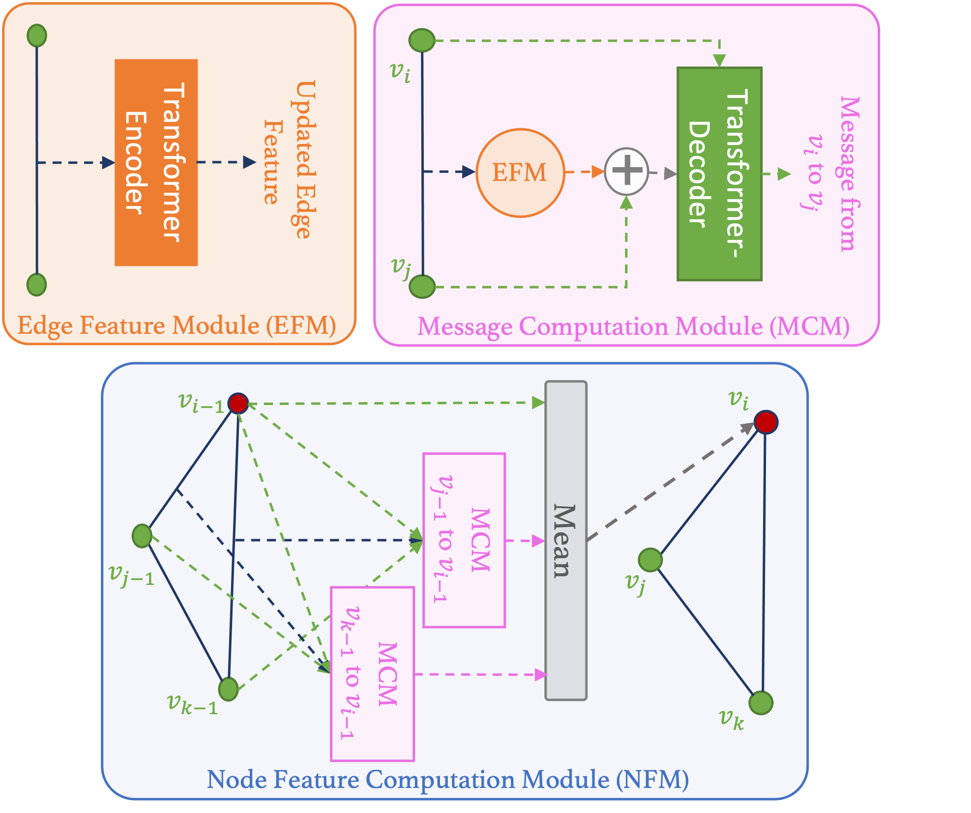
Figure 3: Graph-CoVis Message Passing. The Message Computation Module (MCM) computes incoming messages for each node. First, the Edge Feature Module (EFM) updates the edge representations with a single layer transformer. Then, the messages are computed through a transformer decoder, where the existing node representation attends to a concatenation of the edge representation and the adjacent nodes’ embedding.

$$\mathbf{x}_{i}^{l}=\dfrac{1}{deg(i)}\sum_{j\in\mathcal{N}(i)}m_{j\rightarrow i}^{l},$$ (3)

where $j\in\mathcal{N}(i)$ represents the graph neighborhood of node $v_{i}$, and $deg(i)$ is the number of edges incident to node $v_{i}$.

3.4.2 Co-Visibility, Angular Correspondence, and Floor-Wall Boundary

We estimate dense column-wise representations of co-visibility, correspondence, and layout geometry similar to CoVisPose. Specifically, the edge features at the output of the final message passing layer are mapped to the dense column-wise outputs through a single fully connected layer, $\theta_{DC}$,

$$[\boldsymbol{\phi}^{ij},\boldsymbol{\alpha}^{ij},\mathbf{p}^{ij}]=\theta_{DC}(\mathbf{e}_{ij}^{L}),$$ (4)

where $\boldsymbol{\phi}^{ij}$,$\boldsymbol{\alpha}^{ij},\mathbf{p}^{ij}$ are the column-wise vertical floor-wall boundary angle, angular correspondence, and co-visibility probability, respectively, and $\mathbf{e}_{ij}^{L}$ are the edge features at the output of the last layer, $L$. Again, we initialize $\theta_{DC}$ with weights from a pre-trained CoVisPose model. Learning these quantities along the edges encourages the edge features to embed information important for relative pose regression, which the node embeddings may then attend to in order to retain information relevant to global pose regression within the group of panoramas.

3.4.3 Pose Decoder

To decode the node embeddings into the 4-parameter pose estimates, we apply three fully connected layers ($\theta_{P}$,), with Mish activation functions [16] between the first two layers.

$$[\mathbf{r}_{i},\mathbf{t}_{i}]=\theta_{P}(\mathbf{x}_{i}^{L}).$$ (5)

3.5 Training

We train and evaluate our model on ZInD [4], which is a large-scale dataset of real homes, containing multiple co-localized panoramas, with layout annotations necessary to support our layout-based correspondence and co-visibility representation. To create our dataset, we aggregate all spaces from ZInD containing three or more co-localized panoramas. For the purpose of training and due to memory limitations, we set the maximum number of panoramas in a cluster to be five.

During training, as large open spaces often contain much more than five panoramas, we randomly sample clusters of three, four, and five panoramas from these larger groups. For a set with $N$ panoramas, the model predicts $N$ global poses. Note that a single model is trained for all $N$ and the number of outputs from the model is determined by the number of input panoramas. We further apply random rotation augmentation, shifting the panoramas horizontally. Further, node ordering is permutated to yield a randomly selected origin node each time. Both types of augmentation result in altered coordinate systems and poses, presenting the network with varying pose targets during training. We use the publicly released train/test/validation split and train for 200 epochs, selecting the best model by validation error.

3.6 Loss Functions

The loss function is composed of two main components, the node loss and the edge loss. The node loss, $\mathcal{L}_{\text{n}}$ itself consists of two terms global node loss $\mathcal{L}_{\text{ng}}$ and relative node loss $\mathcal{L}_{\text{nr}}$. We first directly minimize the pose error in a global coordinate system centered at the origin panorama through the global node loss,

$$\mathcal{L}_{\text{ng}}=\sum_{i=2}^{N}(\|\mathbf{r}_{i}-\hat{\mathbf{r}_{i}}\|_{2}^{2}+\|\mathbf{t}_{i}-\hat{\mathbf{t}}_{i}\|_{2}^{2}),$$ (6)

where N represents the number of nodes in the graph.

Additionally, the relative node loss is designed to encourage global consistency, we formulate this $\mathcal{L}_{\text{nr}}$ between all node estimates, $\hat{\mathbf{r}}_{ij},\hat{\mathbf{t}}_{ij}$ and minimize the error against the ground truth relative poses. This adds extra constraints between nodes other than the origin node. The relative pose node loss is

$$\mathcal{L}_{\text{nr}}=\sum_{i}^{N}\sum_{j\neq i}^{N}(\|\mathbf{r}_{ij}-\hat{\mathbf{r}_{ij}}\|_{2}^{2}+\|\mathbf{t}_{ij}-\hat{\mathbf{t}}_{ij}\|_{2}^{2}).$$ (7)

The combined node loss is

$$\mathcal{L}_{\text{n}}=\mathcal{L}_{\text{ng}}+\beta_{r}\cdot\mathcal{L}_{\text{nr}},$$ (8)

where $\beta_{r}$ is a constant controlling the relative influence of the global vs. relative pose losses, which we set to $0.1$.

The edge loss, $\mathcal{L}_{e}$, is applied to the dense co-visibility, correspondence, and layout geometry estimates as in[11],

$$\mathcal{L}_{\text{e }}=\beta_{ac}\mathcal{L}_{ac}+\beta_{b}\mathcal{L}_{b}+\beta_{cv}\mathcal{L}_{cv}.$$ (9)

The losses related to the other predicted outputs are,

$$\mathcal{L}_{\text{b}}=\sum_{i=1}^{N}\sum_{j=1}^{N}\|\boldsymbol{\phi}_{ij}-\hat{\boldsymbol{\phi}}_{ij}\|_{1},j\neq i$$ (10)

$$\mathcal{L}_{\text{ac}}=\sum_{i=1}^{N}\sum_{j=1}^{N}\|\boldsymbol{\alpha}_{ij}-\hat{\boldsymbol{\alpha}}_{ij}\|_{1},j\neq i$$ (11)

$$\mathcal{L}_{\text{cv}}=\sum_{i=1}^{N}\sum_{j=1}^{N}BCE(\mathbf{p}_{ij},\hat{\mathbf{p}}_{ij}),j\neq i,$$ (12)

where $\mathcal{L}_{\text{b}},\mathcal{L}_{\text{ac}},\mathcal{L}_{\text{cv}}$, are the layout boundary, angular correspondence, and co-visibility losses, respectively and $BCE$ is the binary cross entropy loss.

3.7 Global origin selection

During the training phase, the first panorama in the input list is considered the origin. At inference time, we run the model $\mathbf{N}$ times, with each panorama at the origin, retaining the result where the origin node has the highest mean co-visibility score to the neighboring panoramas.

Group-Size	Methods	Rotation			Translation
		$\operatorname{Mn}\left({}^{\circ}\downarrow\right)$	$\operatorname{Med}\left({}^{\circ}\downarrow\right)$	$\operatorname{Std}({}^{\circ}\downarrow)$	$\operatorname{Mn}\left(\operatorname{m.}\downarrow\right)$	$\operatorname{Med}\left(\operatorname{m.}\downarrow\right)$	$\operatorname{Std}(\operatorname{m.}\downarrow)$
Three	CoVisPose + Greedy	2.648	1.028	11.425	0.093	0.052	0.244
	CoVisPose + PGO	3.156	0.984	12.272	0.109	0.047	0.354
	Graph-CoVis	2.001	0.845	9.146	0.081	0.038	0.292
Four	CoVisPose + Greedy	3.908	1.161	16.557	0.142	0.068	0.370
	CoVisPose + PGO	6.034	1.310	17.773	0.218	0.067	0.581
	Graph-CoVis	3.192	0.941	13.359	0.153	0.061	0.430
Five	CoVisPose + Greedy	3.490	1.257	13.928	0.154	0.078	0.344
	CoVisPose + PGO	8.281	1.715	18.830	0.282	0.089	0.619
	Graph-CoVis	3.294	1.073	12.037	0.172	0.082	0.384

Table 1: Statistics of the rotation and translation error based on ARE and ATE metrics on group of three, four, and five panoramas for presented baselines and Graph-Covis.

4 Experiments

Group-Size	Connection	#Test	Methods	Rotation			Translation
				$\operatorname{Mn}\left({}^{\circ}\downarrow\right)$	$\operatorname{Med}\left({}^{\circ}\downarrow\right)$	$\operatorname{Std}({}^{\circ}\downarrow)$	$\operatorname{Mn}\left(\operatorname{m.}\downarrow\right)$	$\operatorname{Med}\left(\operatorname{m.}\downarrow\right)$	$\operatorname{Std}(\operatorname{m.}\downarrow)$
Three	Partially	52	108	CoVisPose + Greedy	7.849	1.991	18.743	0.308	0.095	0.641
				CoVisPose + PGO	15.744	7.971	21.691	0.685	0.283	1.218
				Graph-CoVis	5.362	1.364	15.923	0.340	0.124	0.993
	Fully	1203	2886	CoVisPose + Greedy	2.423	1.007	10.944	0.084	0.051	0.205
				CoVisPose + PGO	2.612	0.948	11.386	0.084	0.046	0.228
				Graph-CoVis	1.856	0.833	8.706	0.069	0.037	0.208
Four	Partially	108	236	CoVisPose + Greedy	6.776	1.671	21.307	0.267	0.089	0.638
				CoVisPose + PGO	16.573	6.070	25.851	0.585	0.215	1.061
				Graph-CoVis	9.008	1.403	25.240	0.386	0.137	0.811
	Fully	437	1160	CoVisPose + Greedy	3.199	1.069	15.071	0.111	0.064	0.256
				CoVisPose + PGO	3.429	1.045	13.949	0.127	0.056	0.319
				Graph-CoVis	1.754	0.870	7.397	0.095	0.052	0.226
Five	Partially	133	371	CoVisPose + Greedy	4.996	1.575	16.529	0.210	0.095	0.459
				CoVisPose + PGO	16.371	6.528	23.914	0.518	0.229	0.838
				Graph-CoVis	4.713	1.320	13.568	0.246	0.126	0.462
	Fully	219	609	CoVisPose + Greedy	2.584	1.107	11.986	0.120	0.070	0.244
				CoVisPose + PGO	3.368	1.028	12.599	0.139	0.063	0.367
				Graph-CoVis	2.433	0.948	10.915	0.128	0.064	0.319

Table 2: Mean rotation and translation error for groups of three, four, and five panoramas divided into Fully and Partially co-visible sub-sets. The number of training and test examples are shown for each sub-set.

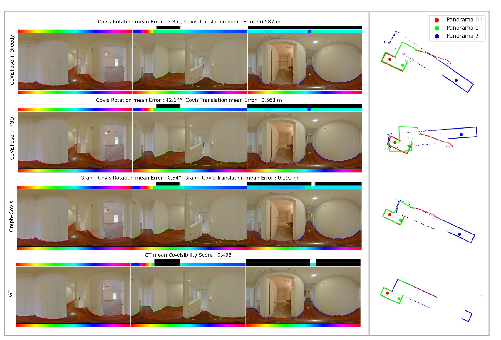
Figure 4: Visualization for both baselines and Graph-CoVis model. The red node represents the common origin node for all approaches. Graph-covis shows improvement in the mean rotation, translation error, and top-down alignment of predicted room boundaries. More examples are in the supplementary material.

We compared our model against standard ways of extending the pair-wise pose estimates to multiple views with experiments on the ZInD data set.

4.1 Baseline

We compare our model to two baseline methods based on the most recent and accurate pose estimation model for panorama images. CovisPose[11] has been demonstrated to be significantly better than alternatives for the domain of upright panorama images, under planar camera motion.

Taking a graph view of the problem with global poses representing nodes and relative pair-wise poses representing edges, we use two standard methods to extend pair-wise relative pose estimates from the CoVisPose model.

Greedy spanning tree. We sort the pair-wise poses by their predicted covisibility and add them greedily from highest covisibility to lowest until all panoramas are placed in the graph. This baseline is called CoVisPose + Greedy.

Pose graph optimization. The most common method to estimate global poses with multiple relative pair-wise poses is to use pose graph optimization (PGO)[5]. We use the graph structure from the greedy spanning tree baseline along with the edge that was not considered (lowest covisibility relative pose) as the pose graph and perform optimization. We call this baseline CoVisPose + PGO.

4.2 Evaluation Metric

To compute the error between ground truth and predicted poses for the panoramas, which are in arbitrary coordinate frames, we compute an alignment transformation between the two configurations. Using a least squares fit[1, 25] to align the 2D point-sets ($x_{i}$ and $y_{i}$ locations of each panorama $i$ in the triplet), we first estimate a transformation matrix (rotation and translation in 2D space) to best align the ground truth and predicted poses. The difference between the positions and orientations of the aligned poses are reported as absolute translation error (ATE) and absolute rotation error (ARE).

4.3 Quantitative Results

The results for mean, median, and standard deviation of the ARE and ATE, separated by the number of panoramas in the set, are shown in Table 1. Graph-CoVis performs better than the baselines for group size of three. For group size of four and five, Graph-CoVis performs better in rotation, but comparable or slightly worse in translation. While PGO moderately reduces the median translation error for group size three and four, PGO performs slightly worse than the greedy method with respect the other metrics. We hypothesize that this is because we ignore the least co-visibility relative pose in the greedy method. Low co-visibilty estimates are also more likely to be erroneous outliers. Including them affects PGO negatively.

To better understand the relation between the graph structure and model, we consider two cases of the connectivity between nodes. Considering the visual overlap between nodes and removing connections between two nodes if overlap is less than a threshold of $0.1$, we have two possible graph structures: fully and partially connected sets.

Two panoramas are deemed to be connected if there is visual connectivity between them. A set of panoramas is fully connected if every pair in that set is visually connected, i.e., the ground truth co-visibility [11] between them is greater than the threshold. It is partially connected if there is at least one pair that is not visually connected. Table 2 shows that in general, Graph-Covis performs better than the baselines for Fully connected examples. The table also shows an interesting correlation between accuracy and the number of training examples in each set.

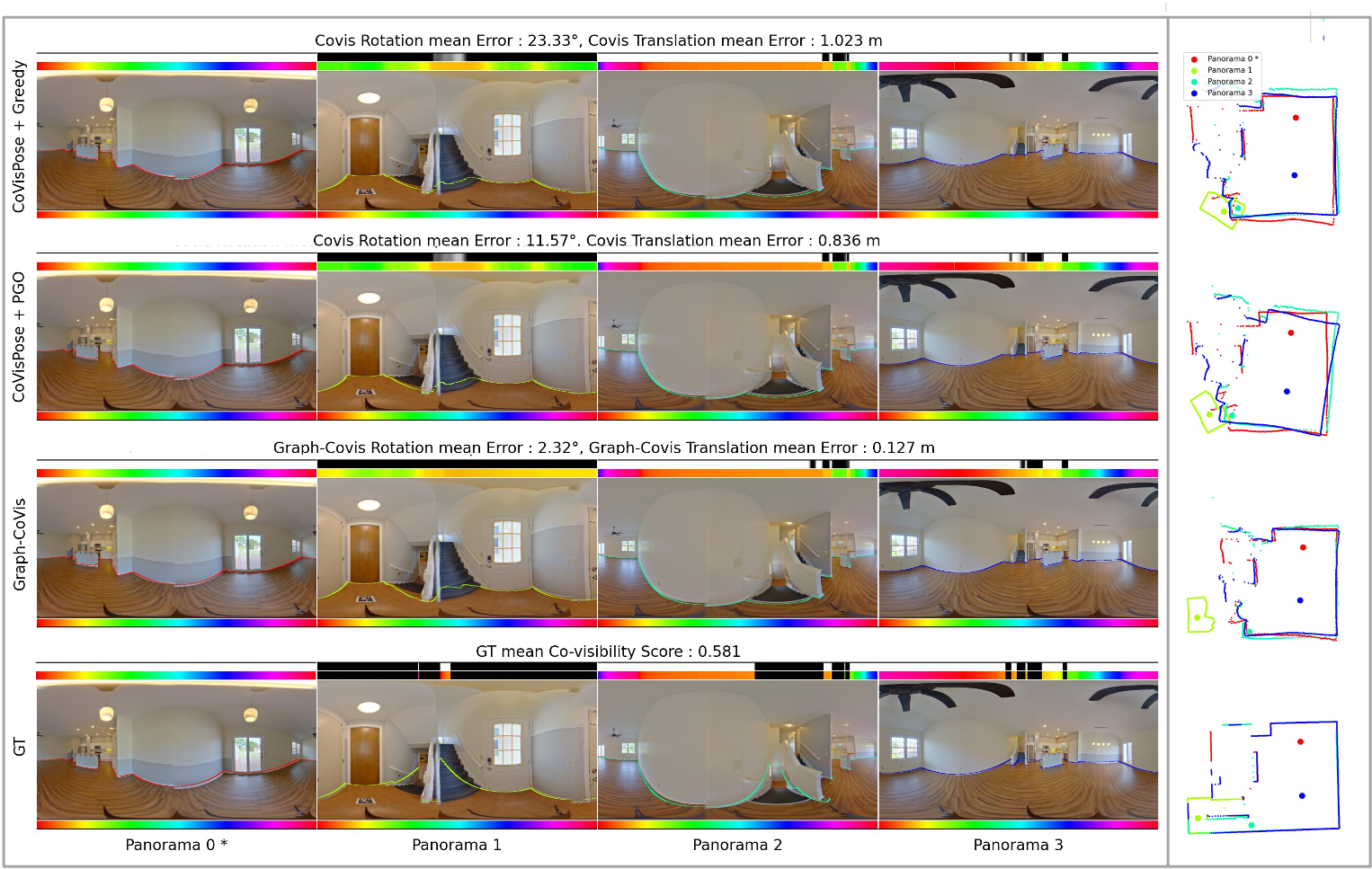
Figure 5: An example result for cluster size four.

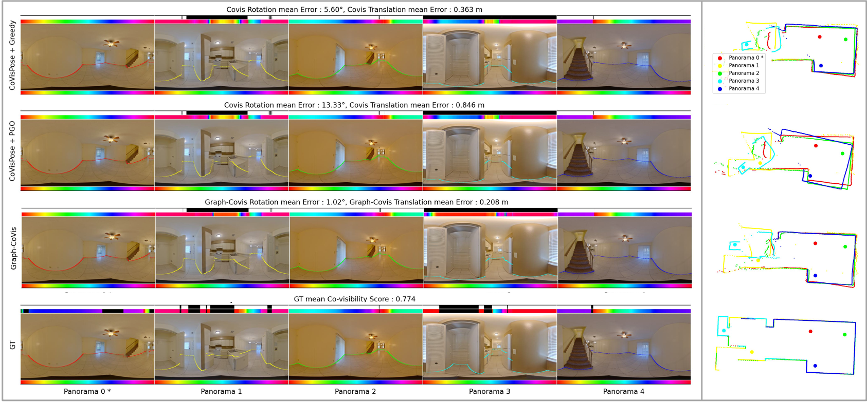
Figure 6: An example result for cluster size five.

4.4 Qualitative Results

Figure 4 shows a typical example triplet and the predicted pose and geometry from the baseline methods and Graph-CoVis. The first column is the panorama, selected as origin node. Above each image the binary strip indicates the predicted co-visibility to the the origin panorama. The color strips at the top (and bottom) of each image indicate the matching angular correspondence from the current panorama to the origin panorama (and origin panorama to current panorama). Predicted boundaries are shown in colored lines within each image. The top-down view of the panorama poses (large dots) and the boundary predictions are shown in the last column. The rows correspond to CoVisPose + Greedy, CoVisPose + PGO, Graph-CoVis, and ground truth. Graph-Covis results in more accurate placement of the panorama poses as well as predicted boundary points.

Figures 5 and 6 show inference examples of having four and five panoramas in the group.

5 Limitations

The CoVisPose representations of dense co-visibility, angular correspondence, and layout boundary, required to train our method, are derived from annotated room layouts, which are not available for some datasets. This limitation precludes the application of our method in absence of re-annotation. Further, these representations, as well as the planar motion model used by our method, exploit the upright camera and fixed camera height assumptions. As a result, our method is not directly applicable to handheld captures.

6 Conclusion

We show that Graph-Covis is a generalization of two-view panorama pose estimation to multi-views. It results in an end-to-end trainable network that directly predicts global poses from an input set of images.

References

- [1] K. S. Arun, T. S. Huang, and S. D. Blostein. Least-squares fitting of two 3-d point sets. IEEE Transactions on Pattern Analysis and Machine Intelligence, PAMI-9(5):698–700, 1987.
- [2] Eric Brachmann, Alexander Krull, Sebastian Nowozin, Jamie Shotton, Frank Michel, Stefan Gumhold, and Carsten Rother. Dsac - differentiable ransac for camera localization. 2017 IEEE Computer Vision and Pattern Recognition Workshops (CVPR), 2017.
- [3] Kefan Chen, Noah Snavely, and Ameesh Makadia. Wide-baseline relative camera pose estimation with directional learning. 2021 IEEE/CVF Conference on Computer Vision and Pattern Recognition (CVPR), pages 3257–3267, 2021.
- [4] Steve Dias Da Cruz, Will Hutchcroft, Yuguang Li, Naji Khosravan, Ivaylo Boyadzhiev, and Sing Bing Kang. Zillow indoor dataset: Annotated floor plans with 360° panoramas and 3d room layouts. 2021 IEEE/CVF Conference on Computer Vision and Pattern Recognition (CVPR), pages 2133–2143, 2021.
- [5] Frank Dellaert. Factor graphs and GTSAM: A hands-on introduction. Technical report, Georgia Institute of Technology, 2012.
- [6] Daniel DeTone, Tomasz Malisiewicz, and Andrew Rabinovich. Superpoint: Self-supervised interest point detection and description. 2018 IEEE/CVF Conference on Computer Vision and Pattern Recognition Workshops (CVPRW), pages 337–33712, 2018.
- [7] Mihai Dusmanu, Ignacio Rocco, Tomás Pajdla, Marc Pollefeys, Josef Sivic, Akihiko Torii, and Torsten Sattler. D2-net: A trainable cnn for joint description and detection of local features. 2019 IEEE/CVF Conference on Computer Vision and Pattern Recognition (CVPR), pages 8084–8093, 2019.
- [8] Martin A. Fischler and Robert C. Bolles. Random sample consensus: A paradigm for model fitting with applications to image analysis and automated cartography. Commun. ACM, 24(6):381–395, jun 1981.
- [9] Lei Han, Mengqi Ji, Lu Fang, and Matthias Nießner. Regnet: Learning the optimization of direct image-to-image pose registration. ArXiv, abs/1812.10212, 2018.
- [10] Richard Hartley and Andrew Zisserman. Multiple View Geometry in Computer Vision. Cambridge University Press, New York, NY, USA, 2 edition, 2003.
- [11] Will Hutchcroft, Yuguang Li, Ivaylo Boyadzhiev, Zhiqiang Wan, Haiyan Wang, and Sing Bing Kang. Covispose: Co-visibility pose transformer for wide-baseline relative pose estimation in 360◦indoor panoramas. In ECCV, 2022.
- [12] Wei Jiang, Eduard Trulls, Jan Hendrik Hosang, Andrea Tagliasacchi, and Kwang Moo Yi. Cotr: Correspondence transformer for matching across images. 2021 IEEE/CVF International Conference on Computer Vision (ICCV), pages 6187–6197, 2021.
- [13] John Lambert, Yuguang Li, Ivaylo Boyadzhiev, Lambert E. Wixson, Manjunath Narayana, Will Hutchcroft, James Hays, Frank Dellaert, and Sing Bing Kang. Salve: Semantic alignment verification for floorplan reconstruction from sparse panoramas. In ECCV, 2022.
- [14] Xinyi Li and Haibin Ling. Pogo-net: Pose graph optimization with graph neural networks. 2021 IEEE/CVF International Conference on Computer Vision (ICCV), pages 5875–5885, 2021.
- [15] David G. Lowe. Distinctive image features from scale-invariant keypoints. International Journal of Computer Vision, 60:91–110, 2004.
- [16] Diganta Misra. Mish: A self regularized non-monotonic activation function. In BMVC, 2020.
- [17] Jeffri Murrugarra-Llerena, Thiago Lopes Trugillo da Silveira, and Cláudio Rosito Jung. Pose estimation for two-view panoramas based on keypoint matching: a comparative study and critical analysis. 2022 IEEE/CVF Conference on Computer Vision and Pattern Recognition Workshops (CVPRW), pages 5198–5207, 2022.
- [18] Mohamed Adel Musallam, Vincent Gaudillière, Miguel Ortiz del Castillo, Kassem Al Ismaeil, and Djamila Aouada. Leveraging equivariant features for absolute pose regression. 2022 IEEE/CVF Conference on Computer Vision and Pattern Recognition (CVPR), pages 6866–6876, 2022.
- [19] Chethan Parameshwara, Gokul Hari, Cornelia Fermuller, Nitin J. Sanket, and Yiannis Aloimonos. Diffposenet: Direct differentiable camera pose estimation. 2022 IEEE/CVF Conference on Computer Vision and Pattern Recognition (CVPR), pages 6835–6844, 2022.
- [20] Barbara Roessle and Matthias Nießner. End2end multi-view feature matching using differentiable pose optimization. ArXiv, abs/2205.01694, 2022.
- [21] Paul-Edouard Sarlin, Daniel DeTone, Tomasz Malisiewicz, and Andrew Rabinovich. Superglue: Learning feature matching with graph neural networks. 2020 IEEE/CVF Conference on Computer Vision and Pattern Recognition (CVPR), pages 4937–4946, 2020.
- [22] Franco Scarselli, Marco Gori, Ah Chung Tsoi, Markus Hagenbuchner, and Gabriele Monfardini. The graph neural network model. IEEE Transactions on Neural Networks, 20(1):61–80, 2009.
- [23] Mohammad Amin Shabani, Weilian Song, Makoto Odamaki, Hirochika Fujiki, and Yasutaka Furukawa. Extreme structure from motion for indoor panoramas without visual overlaps. 2021 IEEE/CVF International Conference on Computer Vision (ICCV), pages 5683–5691, 2021.
- [24] Jiaming Sun, Zehong Shen, Yuang Wang, Hujun Bao, and Xiaowei Zhou. Loftr: Detector-free local feature matching with transformers. 2021 IEEE/CVF Conference on Computer Vision and Pattern Recognition (CVPR), pages 8918–8927, 2021.
- [25] Grace Wahba. A least squares estimate of satellite attitude. SIAM Review, 7(3):409–409, 1965.
- [26] Haiyan Wang, Will Hutchcroft, Yuguang Li, Zhiqiang Wan, Ivaylo Boyadzhiev, Yingli Tian, and Sing Bing Kang. Psmnet: Position-aware stereo merging network for room layout estimation. In Proceedings of the IEEE/CVF Conference on Computer Vision and Pattern Recognition (CVPR), pages 8616–8625, June 2022.
- [27] Kwang Moo Yi, Eduard Trulls, Vincent Lepetit, and Pascal Fua. Lift: Learned invariant feature transform. CoRR, abs/1603.09114, 2016.