Decoupling Quantile Representations from Loss Function

Abstract

The simultaneous quantile regression (SQR) technique has been used to estimate uncertainties for deep learning models, but its application is limited by the requirement that the solution at the median quantile ($\tau=0.5$) must minimize the mean absolute error (MAE). In this article, we address this limitation by demonstrating a duality between quantiles and estimated probabilities in the case of simultaneous binary quantile regression (SBQR). This allows us to decouple the construction of quantile representations from the loss function, enabling us to assign an arbitrary classifier $f({\bm{x}})$ at the median quantile and generate the full spectrum of SBQR quantile representations at different $\tau$ values. We validate our approach through two applications: (i) detecting out-of-distribution samples, where we show that quantile representations outperform standard probability outputs, and (ii) calibrating models, where we demonstrate the robustness of quantile representations to distortions. We conclude with a discussion of several hypotheses arising from these findings.

1 Introduction

Deep learning models have become ubiquitous across diverse domains, and are increasingly being used for several critical applications. Common questions which arise in practice are - (a) Can this model be used on the given data input? and (b) If so, how much can one trust the probability prediction obtained? The former refers to the problem of Out-of-Distribution (OOD) detection [18, 12] and the latter refers to the problem of Calibration [14, 24, 27]. Understanding the implications of a deep learning model is also a topic of current research [35, 9, 30, 20].

Quantile regression techniques [21, 22] provide much richer information about the model, allowing for more comprehensive analysis and understanding relationship between different variables. However, these techniques aren’t widely used in modern deep learning based systems since [7] - (a) The loss function is restricted to be mean absolute error (MAE) or the pinball loss. This might not compatible with domain specific losses. (b) Moreover, it is difficult to optimize the loss function (due to non-convex nature). (c) Adapting the quantile regression approach for classification is also challenging due to piecewise constant behavior of the loss function. In [38] the authors show how simultaneous quantile regression (SQR) techniques can be used to estimate the uncertainties of the deep learning model in the case of regression problems.

Motivation and Contributions: In this article we decouple the construction of the quantile representations and the choice of loss function by identifying the Duality property between quantiles and probabilities. We leverage the duality to construct Quantile-Representations for any given classifier $f({\bm{x}})$ in section 3.1. Such quantile representations are shown to capture the training distributions in section 4.2. We show that these representations outperform the baseline for OOD detection in section 4.3. We also show that quantile-representations predict probabilities which are invariant to distortions in section 4.4. Proof-of-concept experiments to improve OOD detection (appendix C), illustrating the insufficiency of existing calibration techniques (appendix D) and identifying distribution shifts within the data (appendix E) are discussed in the appendix.

Illustrating the Construction of Quantile Representations:

Before diving into the rigorous definition of quantile representations, we illustrate the construction using a simple toy example. Figure 1(a) shows a simple toy example with 3 classes - $0,1,2$. Class $0$ is taken to be out-of-distribution (OOD), while classes $1,2$ are taken to in-distribution (ID). To get the quantile representation - (step 1) we first construct a simple classifier to differentiate classes $1,2$, (step 2) To get a classifier at quantile $\tau$, construct $y_{i}^{+}=I[p_{i}>\tau]$, where $p_{i}$ denotes the predicted probability in (step 1). Construct a classifier using the new labels $y_{i}^{+}$. Figure 1(b) illustrates the classifiers obtained at different $\tau$. In (step 3) concatenate the outputs (predictions) of all the classifiers at different $\tau$ to get the quantile-representations.

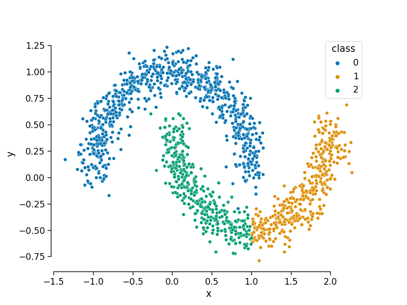
(a) Original Data

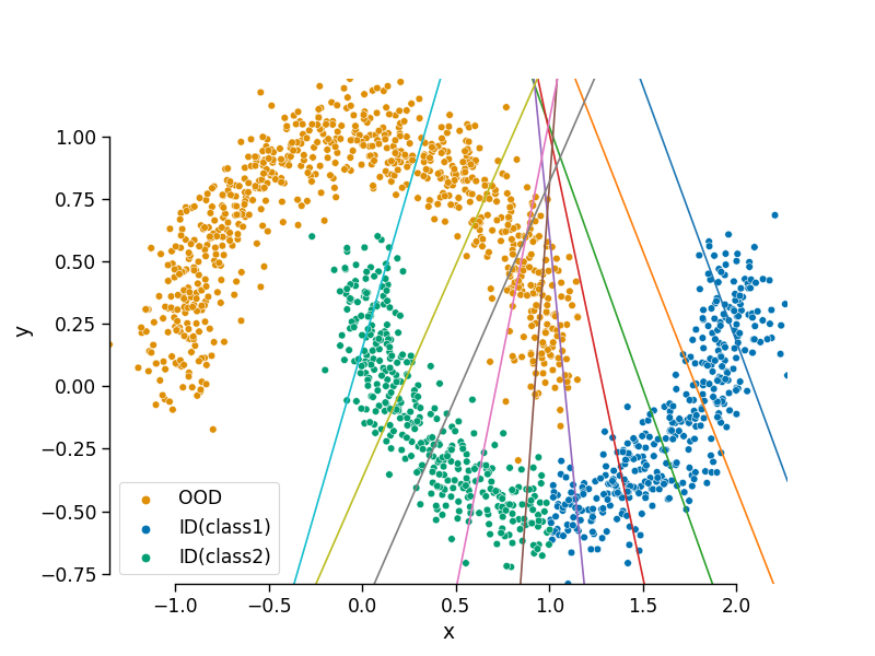
(b) Classifiers at different quantiles ($\tau$)

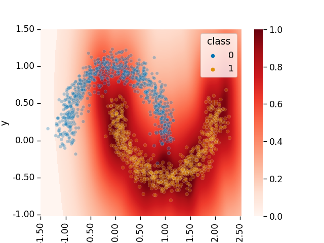
(c) OOD Detection with Quantile-Representations

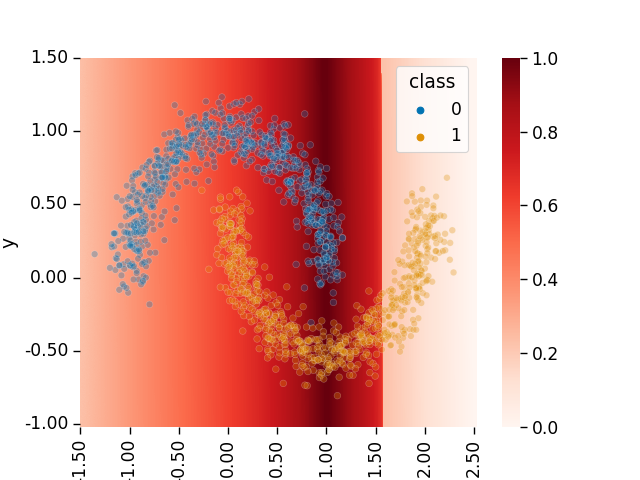
(d) OOD Detection using single classifier predictions

Figure 1: Illustrating the construction of Quantile Representations. (a) Simple toy example. (b) Illustrates different classifiers obtained for different $\tau$. (c) OOD detection using Quantile Representations. (d) OOD detection using the predictions from a single classifier. The brightness of Red indicates the score of a point being in-distribution (ID). Observe that, in this case, quantile-representations are able to differentiate the in-distribution (ID) vs out-of-distribution (OOD).

The quantile representations obtained through our approach can be applied to a variety of situations. As an example, we demonstrate their use in out-of-distribution (OOD) detection, as shown in Figure 1(c). We use the One-Class-SVM method from scikit-learn ([36]) for OOD detection. Figure 1(c) illustrates that the quantile representations are able to differentiate between in-distribution (ID) and OOD samples. In contrast, Figure 1(d) shows the OOD detection performance using the standard outputs from the median classifier.

Remark: It is worth noting that the construction of quantile representations described above does not rely on a specific loss function, but rather on a “base-classifier” and the thresholding of its predictions. This procedure is based on a duality between quantiles and probabilities, which is discussed in more detail in Section 2. Intuitively, the information captured by quantile representations can be thought of as the “aspects of the feature space that the classifier uses for classification,” which is expected to be greater than the information contained in probabilities, but less than the entire feature space. As we will see in the rest of this article, this information is sufficient for improving out-of-distribution detection and estimating the calibration error of a given classifier.

2 Simultaneous Binary Quantile Regression (SBQR)

The construction of quantile representations shown in Figure 1 is made possible by the duality observed in the case of simultaneous binary quantile regression (SBQR). In this section, we present the theoretical foundations for constructing these quantile representations.

Let $p_{\rm{data}}(X,Y)$, denote the distribution from which the data is generated. $X$ denotes the features and $Y$ denotes the targets (class labels). A classification algorithm predicts the latent Logits $Z$ which are used to make predictions on $Y$.

Let ${\bm{x}}\in{\mathbb{R}}^{d}$ denote the $d$ dimensional features and $y\in\{0,1,\cdots,k\}$ denote the class labels (targets). We assume that the training set consists of $N$ i.i.d samples $\mathcal{D}=\{({\bm{x}}_{i},y_{i})\}$. Let $\hat{{\bm{z}}_{i}}=f({\bm{x}};\theta)$ denote the classification model which predicts the logits ${\bm{z}}_{i}$. In binary case, applying the $\sigma$ (Sigmoid) function we obtain the probabilities, $p_{i}=\sigma({\bm{z}}_{i})$. For multi-class classification we use the $\mathrm{softmax}({\bm{z}}_{i})$ to obtain the probabilities. The final class predictions are obtained using the $\operatorname*{arg\,max}_{k}p_{i,k}$, where $k$ denotes the class-index.

2.1 Review - Quantile Regression and Binary Quantile Regression

Let $F_{Y}(y)=P(Y\leq y)$ denote the cumulative distribution of a random variable $Y$. $F_{Y}^{-}(\tau)=\inf\{x:F_{Y}(y)\geq\tau\}$ denotes the quantile distribution of the variable $Y$, where $0<\tau<1$. The aim of quantile regression is to predict the $\tau^{th}$ quantile of the variable $Y$ given the features ${\bm{x}}$, that is to estimate $f_{\tau}(x)\approx F_{Y}^{-}(\tau\mid X=x)$. This is achieved by minimizing pinball-loss or check-loss [21]

$$\rho(\hat{y},y;\tau)=\begin{cases}\tau(y-\hat{y})&\text{if }(y-\hat{y})>0\\ (1-\tau)(\hat{y}-y)&\text{otherwise }\\ \end{cases}$$ (1)

When $\tau=0.5$, we obtain the loss to be equivalent to mean absolute error (MAE).

Quantile Regression for Classification:

The above formulation is used when the target $Y$ is continuous. In binary classification, since $Y\in\{0,1\}$ is discrete, replace $\hat{y_{i}}=p_{i}$ and use loss in equation 1. For the multi-class case we follow the one-vs-rest procedure by encoding the target as one-hot-vector. If the class label is $k$, take $Y={\bm{e}}_{k}$ where ${\bm{e}}_{k}(i)=1$ if $i=k$, and $0$ otherwise. The check-loss is applied to each entry separately, and take sum over all entries.

Simultaneous Quantile Regression (SQR):

The loss in equation 1 is for a single $\tau$. One can instead minimize the expected loss over all $\tau\in(0,1)$,

$$\mathbb{E}_{\tau\sim U[0,1]}[\rho(\hat{y},y;\tau)]$$ (2)

This is referred to as simultaneous quantile regression (SQR). Using the loss in equation 2 instead of equation 1 enforces the solution to have monotonicity property [38]. If ${\mathcal{Q}}({\bm{x}},\tau)$ denotes the solution to equation 2, monotonicity requires

$${\mathcal{Q}}({\bm{x}},\tau_{i})\leq{\mathcal{Q}}({\bm{x}},\tau_{j})\Leftrightarrow\tau_{i}\leq\tau_{j}$$ (3)

The classification variant for the loss equation 2 assumes $y\in\{0,1\}$ and ${\mathcal{Q}}({\bm{x}},\tau)\in(0,1)$. To differentiate with SQR, we refer to this as Simultaneous Binary Quantile Regression (SBQR).

Remark: ${\mathcal{Q}}({\bm{x}},\tau)$ is sometimes written as ${\mathcal{Q}}({\bm{x}},\tau;\theta)$, where $\theta$ indicates the parameters (such as weights in a neural neural network). For brevity, we do not include the parameters $\theta$ in this article.

3 Quantile Representations

Note that for a fixed ${\bm{x}}_{i}$, the solution to equation 2 gives ${\mathcal{Q}}({\bm{x}}_{i},\tau)$ which is a function of $\tau$. ${\mathcal{Q}}({\bm{x}}_{i},\tau)$ can be interpreted as representation assigned to each ${\bm{x}}_{i}$. We refer to this as Quantile Representation. A natural question arises - What information does quantile representations encode?

Informally, quantile representation ${\mathcal{Q}}({\bm{x}}_{i},\tau)$ encode all information relevant to the classification of ${\bm{x}}_{i}$. This is greater than fixing ${\mathcal{Q}}({\bm{x}}_{i},0.5)$ (fixing $\tau$=0.5 gives us median classifier) and less than the information present in the distribution of features. To understand this difference, consider the toy example in figure 1. Figure 1(d) considers only the predictions at ${\mathcal{Q}}({\bm{x}}_{i},0.5)$, and fails to identify the out-of-distribution (OOD) samples. Quantile representations in figure 1(c) identifies the trained samples perfectly. An example where quantile representations cannot identify the distribution from the train data is discussed in appendix C.

Since ${\mathcal{Q}}({\bm{x}}_{i},\tau)$ encode information relevant to the classification of ${\bm{x}}_{i}$, this allows us to analyze the “reasons” for assigning a particular class to ${\bm{x}}_{i}$. Specifically, this information can help us identify if a particular sample is out-of-distribution (OOD detection) and also to estimate the confidence of our prediction (Calibration). We verify this in section 4.4.

3.1 Generating Quantile Representations Using Duality between Quantiles and Probabilities

Recall that ${\mathcal{Q}}({\bm{x}}_{i},\tau)$ minimizes equation 2. This enforces that ${\mathcal{Q}}({\bm{x}}_{i},0.5)$ should minimize the mean absolute error (MAE). This restricts the applications of quantile representations to classifiers trained using MAE. While, using MAE as loss has a lot of advantages [13], it also enforces a bias on the solutions which are not suitable in practice. Most classifiers in practice are trained using domain specific losses using regularization terms. This restricts the application of quantile regression based approaches.

We can circumvent this restriction by observing duality between quantiles and estimated probabilities in SBQR. For binary classification, equation 1 can be written as

$$\rho(\hat{y},y;\tau)=\begin{cases}\tau(1-\hat{y})&\text{if }y=1\\ (1-\tau)(\hat{y})&\text{if }y=0\\ \end{cases}$$ (4)

Now, observe that,

$$\rho(\hat{y},y;\tau)=\rho(1-\tau,y;1-\hat{y})$$ (5)

In words, this implies a solution which predicts the $\tau^{th}$ quantile can be interpreted as the quantile at which the probability is $1-\tau$. This observation leads to the algorithm 1 for generating the quantile representations.

Algorithm 1 Generating Quantile Representations.

• Let $\mathcal{D}=\{({\bm{x}}_{i},y_{i})\}$ denote the training dataset. Assume that a pretrained binary classifier $f({\bm{x}})$ is given. The aim is to generate the quantile representations with respect to $f({\bm{x}})$. We also refer to this $f({\bm{x}})$ as base-classifier.

• Assign ${\mathcal{Q}}({\bm{x}},0.5)=f({\bm{x}},;\theta)$, that is take the median classifier to be the given classifier.

• Define $y_{i,\tau}^{+}=I[f({\bm{x}}_{i})>(1-\tau)]$. We refer to this as modified labels at quantile $\tau$.

• To obtain ${\mathcal{Q}}({\bm{x}},\tau)$, train the classifier using the dataset $\mathcal{D}_{\tau}^{+}=\{({\bm{x}}_{i},y_{i,\tau}^{+})\}$. Repeating this for all $\tau$ allows us to construct the quantile representation ${\mathcal{Q}}({\bm{x}},\tau)$.

Why does algorithm 1 return quantile representations?

Assume for a arbitrary ${\bm{x}}_{i}$, we have ${\mathcal{Q}}({\bm{x}}_{i},0.5)=p_{i}$. Standard interpretation states - at quantile $\tau=0.5$, the probability of ${\bm{x}}_{i}$ in class $1$ is $p_{i}$. However, thanks to duality in equation 5, this can also be interpreted as - At quantile $\tau=(1-p_{i})$, the probability of ${\bm{x}}_{i}$ in class $1$ is 0.5.

Thanks to monotonocity property in equation 3, we have for all $\tau<(1-p_{i})$, probability of ${\bm{x}}_{i}$ in class $1$ is $<0.5$, and hence belongs to class $0$. And for all $\tau>(1-p_{i})$, probability of ${\bm{x}}_{i}$ in class $1$ is $>0.5$, and hence belongs to class $1$.

This implies that at a given quantile $\tau^{*}$, ${\bm{x}}_{i}$ will belong to class $1$ if $\tau^{*}>(1-p_{i})$ or if $p_{i}>(1-\tau^{*})$ or if $f({\bm{x}}_{i})>(1-\tau^{*})$. Defining, $y_{i,\tau^{*}}^{+}=I[f({\bm{x}}_{i})>(1-\tau^{*})]$, we have that the classifier at quantile $\tau^{*}$, ${\mathcal{Q}}({\bm{x}},\tau^{*})$ fits the data $\mathcal{D}_{\tau}^{+}=\{({\bm{x}}_{i},y_{i,\tau^{*}}^{+})\}$ and thus can be used to identify ${\mathcal{Q}}({\bm{x}},\tau^{*})$. This gives us the algorithm 1 to get the quantile representations for an arbitrary classifier $f({\bm{x}})$.

Remark (Sigmoid vs Indicator function): In theory, we approximate $\hat{y_{i}}=I[\hat{{\bm{z}}_{i}}>0]$ (i.e Indicator function) with the sigmoid as $\hat{y_{i}}=\sigma(\hat{{\bm{z}}_{i}})$. The algorithm 1 gives a solution up to this approximation. In particular we have the following theorem

Theorem 3.1.

Assume that we generate the output using the indicator function $\hat{y_{i}}=I[\hat{{\bm{z}}_{i}}>0]$, instead of sigmoid function $\hat{y_{i}}=\sigma({\bm{z}}_{i})$. Further assume that the base classifier $f({\bm{x}})=\sigma(\phi({\bm{x}}_{i}))$ is obtained using the MAE loss, i.e by minimizing

$$\min_{\phi}\sum_{i}|y_{i}-\sigma(\phi({\bm{x}}_{i}))|$$ (6)

Then the solution ${\mathcal{Q}}({\bm{x}},\tau)$ obtained by algorithm 1 minimizes the cost in equation 2 over the dataset $\mathcal{D}$, i.e

$$\min_{\psi}\mathbb{E}_{\tau\in U[0,1]}\left[\frac{1}{N}\sum_{i=1}^{N}\rho(I[\psi({\bm{x}}_{i},\tau)\geq 0],y_{i};\tau)\right]$$ (7)

A sketch of the proof for the above theorem is given in the appendix A.

To summarize, thanks to the duality in equation 5, one can compute the quantile representations for any arbitrary classifier. This allows for detailed analysis of the classifier and the features learned. In the following section we first discuss the implementation of algorithm 1 in practice and provide both qualitative and quantitative analysis for specific models.

4 Experiments and Analysis

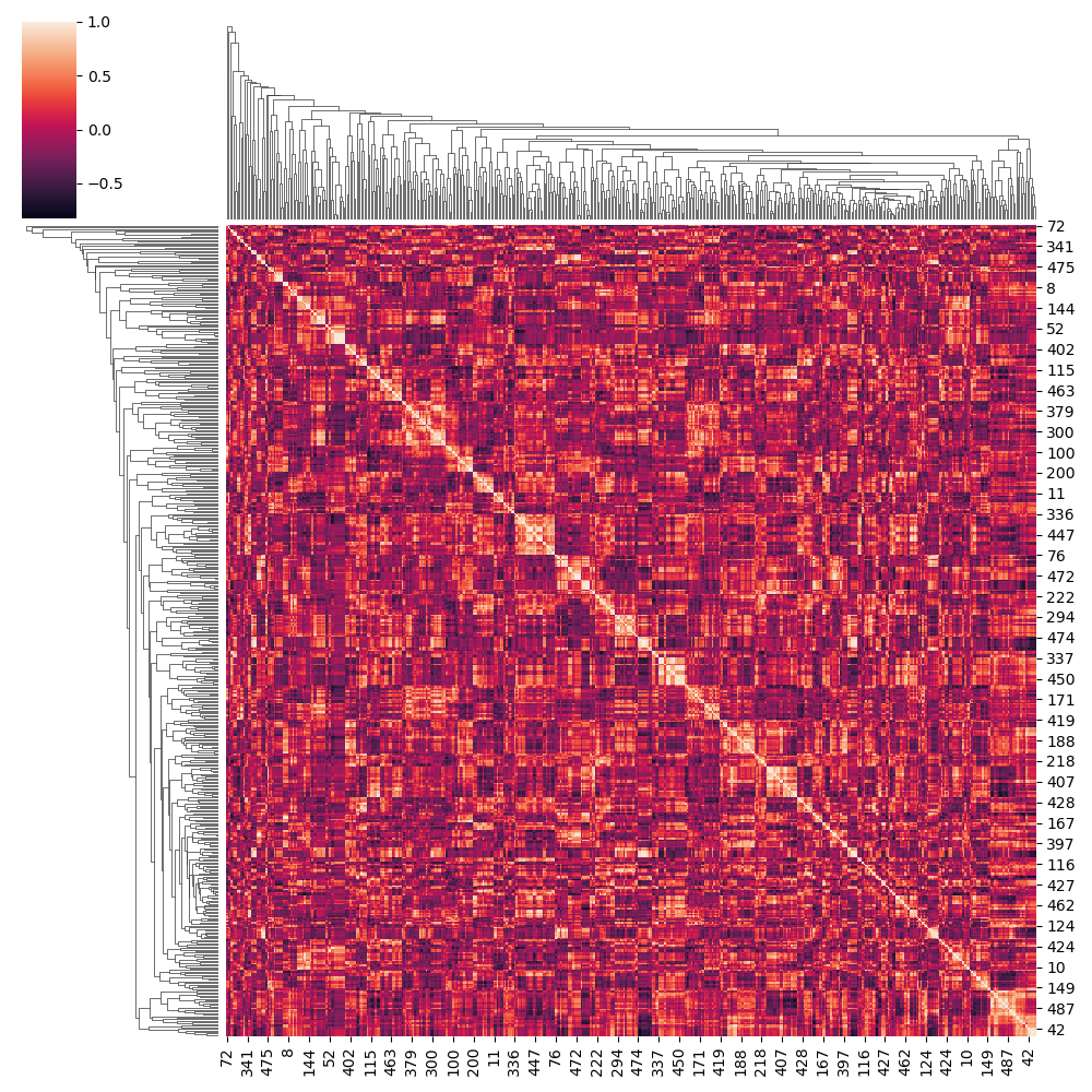
(a) Quantile Representations (Resnet34)

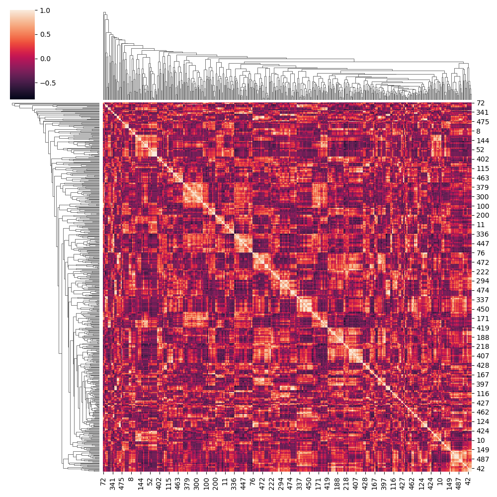
(b) Original Features (Resnet34)

(c) Scatterplot

Figure 2: Do quantile representations capture the relevant information for classification? (a) Cross-correlations obtained using Quantile representations for Resnet34 on CIFAR10 (b) Cross-correlations obtained using train features for Resnet34 on CIFAR10. (c) Scatterplot with best fit line (using Locally Weighted Scatterplot Smoothing[8]) of the cross-correlation of features. Observe that as the correlation becomes important (i.e close to $-1$ or $1$) quantile representations are more consistent with raw features.

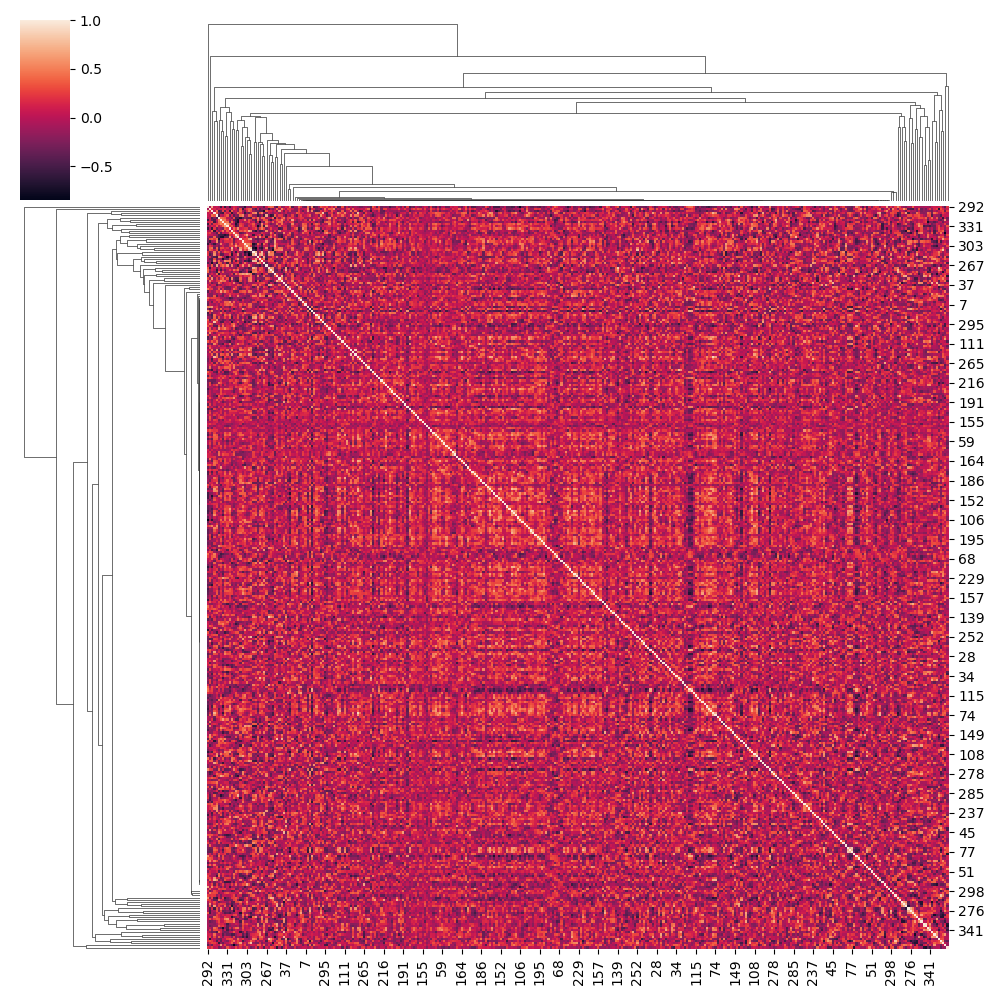
(a) Quantile Representations (Densenet)

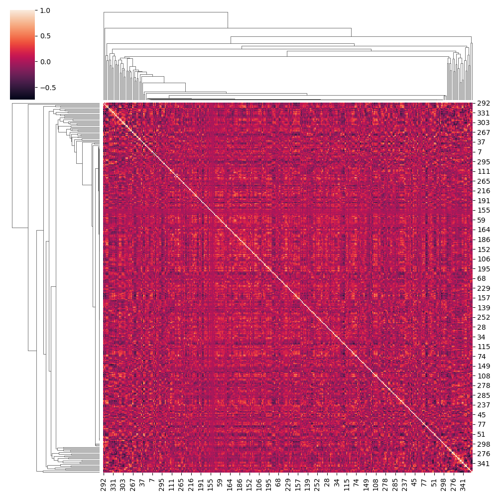
(b) Original Features (Densenet)

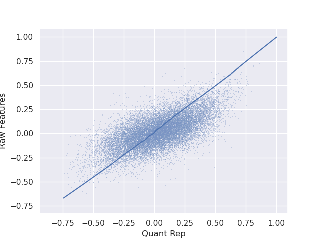
(c) Scatterplot

Figure 3: Do quantile representations capture the relevant information for classification? (a) Cross-correlations obtained using Quantile representations for Densenet on CIFAR10 (b) Cross-correlations obtained using train features for Densenet on CIFAR10. (c) Scatterplot with best fit line (using Locally Weighted Scatterplot Smoothing[8]) of the cross-correlations. Observe that as the correlation becomes important (i.e close to $-1$ or $1$) quantile representations are more consistent with raw features.

4.1 Generating Quantile Representations in practice

To generate the quantile representations in practice we follow algorithm 1 as described with a few modifications as follows. (Remark: Code is attached as supplementary material and will be made public after publication of the manuscript)

Use Logits instead of Probabilities: Observe that both the base-classifier $f({\bm{x}})$ and the quantile representations ${\mathcal{Q}}({\bm{x}},\tau)$ are taken to be probabilities, and hence belong to the interval $(0,1)$. However, in practice we observed precision issues when considering the probability outputs using the $\sigma(.)$ function. Hence we use the logits instead of the probabilities as this reduces the precision problems associates with the $\sigma(.)$ function. Observe that since logits and probabilities are related by a monotonic transformation, this does not make a difference for classification.

Taking discrete quantiles: Observe that the quantile representation ${\mathcal{Q}}({\bm{x}},\tau)$ is a continuous function of $\tau$. In practice we consider $n_{\tau}=1000$ equally spaces quantiles between $0.01$ and $0.99$ as an approximation.

Use one-vs-rest for multi-class classification: The algorithm 1 assumes binary classes. For multi-class classification we use one-vs-rest approach to generate the quantile representations. Accordingly, the quantile representation size would be $n_{\text{classes}}\times n_{\tau}$. Remark: This poses a problem for computational complexity of generating the quantile representations. This is further discussed in section 6.

Using weighted quantiles for multi-class classification: Interpretation of quantile regression coefficients is related to the class distribution. For instance if the number of data points in class $0$ is 200 and class $1$ is 800, the coefficients at quantile $0.8$ are much more meaningful than at quantile $0.5$ [2]. In case of one-vs-rest approach to multi-class classification it is always the case that the classes are imbalanced. To counter this, we use weighted quantiles by assigning weights to the data points inversely proportional to its class size.

Interpolating the quantile representations: To generate quantile representation at each $\tau$, one has to train a classifier. This can lead to increase computational requirement when considering large number of quantiles $\tau$. However the coefficients of the classifiers at different $\tau$ are expected to smoothly vary with $\tau$. Hence, to reduce computational complexity, we generate the coefficients at $100$ distinct $\tau$ equally spaced between $0.01$ and $0.99$ and use cubic-interpolation [15] to generate coefficients for $1000$ quantiles.

Normalizing the coefficients for the classifier Note that if $\beta$ denotes the coefficients of the boundary for linear classifier, then $c\beta$ also defines the same boundary. Since the algorithm involves constructing and comparing different classifiers, we normalize the coefficients of the classifier using the $L^{2}$ norm. This allows for fair comparison of logits across different models.

4.2 Cross-correlation of features

To illustrate that the quantile representations capture the aspects of data-distrbution relevant to classification, we perform the following experiment:

Construct the cross-correlation between features using (i) Quantile Representations and (ii) Feature values extracted using the traindata. If our hypothesis is accurate, then cross-correlations obtained using quantile-representations and feature values would be similar.

In Figures 2 and 3, we present the results of using features from Resnet34 and Densenet on the CIFAR10 dataset. Figures 2(a) and 2(b) show the results for Resnet34, and Figures 3(a) and 3(a) show the results for Densenet. To visualize the cross-correlations, we use a heatmap with row and column indices obtained by averaging the linkage of train features. This index is common for both quantile representations and extracted features. It is evident from the figure that the cross-correlation between features is similar whether it is computed using extracted features or quantile representations.

4.3 OOD Detection

Table 1: Comparison of Quantile-Representations with baseline for OOD Detection. Observe that Quantile-Representations outperform the baseline in all the cases.

		DenseNet (Baseline/Quantile-Rep)
		LSUN(C)	LSUN(R)	iSUN	Imagenet(C)	Imagenet(R)
CIFAR10	AUROC	92.08/93.64	93.86/94.61	92.84/93.74	90.93/91.72	90.93/92.06
	TNR@TPR95	58.19/64.56	63.07/66.89	59.64/64.68	53.94/56.34	54.44/58.22
	Det. Acc	85.58/87.14	87.66/88.60	86.29/87.42	84.11/84.93	84.10/85.33
SVHN	AUROC	91.80/92.29	90.75/90.70	91.21/91.30	91.93/91.97	91.93/92.01
	TNR@TPR95	54.61/58.77	47.67/48.55	48.24/50.15	52.38/53.68	52.43/53.64
	Det. Acc	85.10/85.37	84.32/84.16	84.80/84.77	85.42/85.55	85.46/85.50
		Resnet34 (Baseline/Quantile-Rep)
CIFAR10	AUROC	91.43/91.76	92.64/93.08	91.89/92.34	90.59/90.81	89.12/89.39
	TNR@TPR95	54.96/56.76	63.24/65.75	58.56/60.94	52.86/54.89	47.41/49.93
	Det. Acc	84.63/84.96	85.41/86.06	84.39/85.17	83.24/83.44	81.74/82.05
SVHN	AUROC	94.80/94.87	94.37/94.46	95.13/95.22	95.73/95.85	95.62/95.70
	TNR@TPR95	76.19/76.15	72.10/72.87	75.88/76.25	79.16/79.53	78.34/78.82
	Det. Acc	89.58/89.72	88.82/88.87	89.78/89.85	90.72/90.87	90.54/90.60

An assumption made across all machine learning models is that - Train and test datasets share the same distributions. However, test data can contain samples which are out-of-distribution (OOD) whose labels have not been seen during the training process [30]. Such samples should be ignored during inference. Hence OOD detection is a key component of different ML systems. Several methods [18, 25, 3] have been proposed for OOD detection. Here we check how quantile representations compare to the baseline method in [18] for OOD detection.

Consider the following model for binary classification

$${\bm{z}} =g({\bm{x}})+\epsilon({\bm{x}})$$ (8)

$${\bm{y}} =I[{\bm{z}}\geq 0]$$

where $\epsilon({\bm{x}})$ is some error distribution dependent on ${\bm{x}}$ (for example hetero-skedastic models). The base classifier would then be obtained using $f({\bm{x}})=P(g({\bm{x}})+\epsilon({\bm{x}})\geq 0)$.

Consider a regression problem, that is assume latent ${\bm{z}}$ is known. Then for a test sample ${\bm{x}}_{t}$, $g({\bm{x}}_{t})$ denotes the estimates latent score. If this observed latent score is an outlier with respect to the distribution $\epsilon$, then it is most likely that ${\bm{x}}_{t}$ is OOD sample. However, we do not have the information about the latent scores for the classification problem. Hence the classifier constructed using equation 8 cannot differentiate between OOD samples and samples with high confidence. This is illustrated in figure 1(d).

Quantile representations solve this by constructing different classifiers at different distances from the base-classifier (illustrated in figure 1(b)). This allows us to differentiate between OOD samples and samples with high confidence. Thus we expect quantile representations to improve the OOD detection. This is verified empirically below.

Experimental Setup

For this study, we use the CIFAR10[23] and SVHN[29] datasets as in-distribution (ID) datasets and the iSUN[40], LSUN[41], and TinyImagenet[26] datasets as out-of-distribution (OOD) datasets. To extract features, we employ two network architectures: Resnet34[16] and Densenet[19]. We train a base classifier using Logistic Regression, on the extracted features with the labels, and use this classifier to construct quantile representations. For evaluation we use (i) AUROC: The area under the receiver operating characteristic curve of a threshold-based detector. A perfect detector corresponds to an AUROC score of 100%. (ii) TNR at 95% TPR: The probability that an OOD sample is correctly identified (classified as negative) when the true positive rate equals 95%. (iii) Detection accuracy: Measures the maximum possible classification accuracy over all possible thresholds.

Methodology and Results

The baseline method uses the outputs from the base-classifier and then use Local Outlier Factor (LOF) [4] to identify the OOD samples. The quantile approach uses quantile-representations instead and then use the LOF approach to detect OOD samples. Table 1 shows the results obtained using quantile-representations and outputs from the base classifier. Observe that quantile-representations outperform the baseline approach for detection of OOD samples.

Remark: Observe that the improvement of OOD detection using quantile-representations in Densenet is better than for Resnet34. This is due to the fact that features are much more correlated in Resnet34 (figure 2) compared to Densenet (figure 3). So, the amount of improvement itself can be used to quantify the importance of the features.

Can we improve OOD detection?

Observe that OOD detection problem considers train labels as a guide. In the sense that, OOD samples are defined as the ones which do not belong to train labels. If we generalize this to identifying the train distribution alone - It can be achieved by using random labels along with quantile representations. In fact this method, by suitable sampling the points and assigning pseudo-labels, can identify any region of the space. See appendix C for illustration.

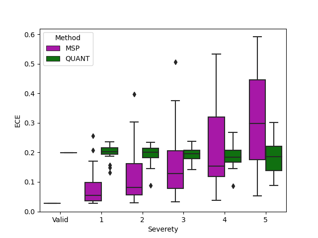
(a) ECE (Resnet34)

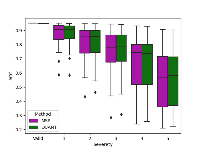
(b) Accuracy (Resnet34)

(c) ECE (Densenet)

(d) Accuracy (Densenet)

Figure 4: Quantile representations can be effective for calibration because they estimate probabilities using Equation equation 13, which has been shown to be robust to corruptions. As demonstrated using the CIFAR10C dataset [17], the Expected Calibration Error (ECE) of the probabilities obtained from quantile representations (QUANT) does not increase with the severity of the corruptions. In contrast, when using the standard Maximum Softmax Probability (MSP) method, the calibration error increases as the severity of the corruptions increases.

4.4 Calibration of ML models

For several applications the confidence of the predictions is important. This is measured by considering how well the output probabilities from the model reflect it’s predictive uncertainty. This is referred to as Calibration.

Several methods [33, 43, 24, 1, 27] are used to improve the calibration of the deep learning models. Most of these methods consider a part of the data (apart from train data) to adjust the probability predictions. However, in [31, 28] it has been shown that most of the calibration approaches fail under distortions. In this section we show that calibration using quantile-representations are invariant to distortions.

A perfectly calibrated model (binary class) will satisfy [14]

$$P({\bm{y}}=1|f({\bm{x}})=p^{*})=p^{*}$$ (9)

For multi-class cases this is adapted to

$$P({\bm{y}}=\operatorname*{arg\,max}_{k}(p_{k})|\max_{k}(f({\bm{x}}))=p^{*})=p^{*}$$ (10)

The degree of miscalibration is measured using Expected Calibration Error (ECE)

$$E[|p^{*}-E[P({\bm{y}}=\operatorname*{arg\,max}_{k}(p_{i,k})|\max_{k}(f({\bm{x}}))=p^{*})]|]$$ (11)

This is computed by binning the predictions into $m$ bins - $B_{1},B_{2},\cdots,B_{m}$ and computing

$$\hat{\texttt{ECE}}=\sum_{i=1}^{m}\frac{|B_{i}|}{n}|\texttt{acc}(B_{i})-\texttt{conf}(B_{i})|$$ (12)

where $\texttt{acc}(B_{i})=(1/|B_{i}|)\sum_{j\in B_{i}}I[{\bm{y}}_{j}=\operatorname*{arg\,max}(p_{j})]$ denotes the accuracy of the predictions lying in $B_{i}$, and $\texttt{conf}(B_{i})=\sum_{j\in B_{i}}\max(f({\bm{x}}_{j}))$ indicates the average confidence of the predictions lying in $B_{i}$.

In the ideal scenario, we have that quantile representations predict perfectly calibrated probabilities as illustrated in the following theorem.

Theorem 4.1.

Assume that the data is generated using the model in equation 8, where $f({\bm{x}})=P(g({\bm{x}})+\epsilon({\bm{x}})\geq 0)$ denotes the base-classifier. Let ${\mathcal{Q}}({\bm{x}},\tau)$ denote the quantile representations obtained on this data. Define the probabilities as

$$P({\bm{y}}=1)=\int_{\tau=0}^{1}I[{\mathcal{Q}}({\bm{x}},\tau)\geq 0]d\tau$$ (13)

The probabilities obtained using equation 13 are perfectly calibrated.

The proof for theorem 4.1 is given in appendix B.

We can use theorem 4.1 as a basis to predict the calibration error using quantile representations (illustrated below), even though, in practice, the model predicted from train data may not be perfectly calibrated.

Experimental Setup

In this study, we employ the CIFAR10 dataset and the Resnet34 and Densenet models to investigate the robustness of classifiers. To evaluate the classifiers’ robustness, we use the distorted CIFAR10 dataset introduced in [17], which contains 15 types of common corruptions at five severity levels. This dataset is a standard benchmark for testing the robustness of classifiers. We use quantile-representations trained on the CIFAR10 training data to assess the generalization performance of the classifiers on the distorted dataset. We compare the performance with Maximum Softmax Probability (MSP) as a baseline and evaluate both accuracy and calibration error. We construct the bins $\{B_{i}\}$ using 5 equally spaced quantiles within the predicted probabilities. The probabilities of each class are predicted using equation 13. (Remark: These probabilities do not add upto 1 since we consider a one-vs-rest approach.)

We present the results in Figure 4. As we increase the severity of the distortions, we observe that the accuracy of both the quantile representations and MSP decreases. However, the probabilities obtained from quantile representations are robust to distortions, as their Expected Calibration Error (ECE) does not increase with severity in the same way as MSP’s does. This indicates that quantile representations can more accurately predict calibration error and are more resistant to distortions.

Remark: An unexpected finding in our experiments was that correcting the probabilities obtained from quantile representations using methods like isotonic regression and Platt scaling did not maintain their robustness to distortions. This result is discussed in more detail in the appendix D.

5 Related Work

[21, 32, 34, 5] provides a comprehensive overview of approaches related to quantile regression and identifying the parameters. [6] extends the quantiles to multi-variate case. [38, 39] use quantile regression based approaches for estimating confidence of neural networks based predictions. [1, 11] uses conformal methods to calibrate probabilities, and is closely related to computing quantiles. [7] proposes a similar algorithm to overcome the restriction to pinball loss for regression problems. [10] generates predictive regions using quantile regression techniques.

6 Conclusion, Limitations and Future work

To summarize, in this article we show the duality between quantiles and probabilities in the case of SBQR. Exploiting the duality, we propose an algorithm to compute quantile representations for any given base classifier. We verify that the quantile representations model the training distribution well both qualitatively (by plotting cross-correlations of the features) and quantitatively (using OOD detection baseline). We further show that the probabilities from quantile representations are robust to distortions. Interestingly, we found that traditional approaches cannot be used to correct the calibration error.

The main limitation of the approach is the computation required for algorithm 1 for large scale datasets. We expect that using a neural network to model the function ${\mathcal{Q}}({\bm{x}},\tau)$ using neural networks can reduce the training time. This is considered for future work. In appendix C we propose using random labels to improve the OOD detection and illustrate it on a toy example. In appendix E we illustrate (on toy example) how distribution shift may be identified using quantile representations. These are considered for future work as well.

Appendix A Proof for theorem 3.1

Let $\mathcal{D}=\{({\bm{x}}_{i},y_{i})\}$ denote the train dataset of size $N$. Then the minima over the dataset $\mathcal{D}$, is obtained by solving,

$$\min_{\psi}\mathbb{E}_{\tau\sim U[0,1]}\left[\frac{1}{N}\sum_{i}\rho(I[\psi({\bm{x}}_{i},\tau)\geq 0],y_{i};\tau)\right]$$ (14)

Let ${\mathcal{Q}}({\bm{x}},\tau)$ denotes the solution obtained using the algorithm 1. Let ${\mathcal{P}}({\bm{x}},\tau)$ denote the solution obtained by solving equation 14.

We aim to show that ${\mathcal{Q}}({\bm{x}}_{i},\tau)=I[{\mathcal{P}}({\bm{x}}_{i},\tau)\geq 0]$ for all the points in $\mathcal{D}=\{({\bm{x}}_{i},y_{i})\}$.

First, observe that, since the base classifier $f({\bm{x}})$ is obtained using MAE we have that ${\mathcal{Q}}({\bm{x}}_{i},0.5)=I[f({\bm{x}}_{i})>0.5]=I[{\mathcal{P}}({\bm{x}}_{i},0.5)\geq 0]$.

Next for arbitrary $\tau$, we show that ${\mathcal{Q}}({\bm{x}}_{i},\tau)=I[{\mathcal{P}}({\bm{x}}_{i},\tau)\geq 0]$ over the dataset $\mathcal{D}=\{({\bm{x}}_{i},y_{i})\}$.

We approximate the indicator function as $I[{\bm{x}}\geq 0]\approx\lim_{k\to\infty}K_{k}({\bm{x}})$. For instance one can consider $K_{k}({\bm{x}})=\sigma({\bm{x}}k)$. Observe that a solution to minimize equation 14 can be obtained by

$${\mathcal{P}}({\bm{x}},\tau)=\lim_{k\to\infty}\operatorname*{arg\,min}_{\psi}\mathbb{E}_{\tau\sim U[0,1]}\left[\frac{1}{N}\sum_{i}\rho\left(K_{k}\left(\psi({\bm{x}}_{i},\tau)\right),y_{i};\tau\right)\right]$$ (15)

Let

$${\mathcal{P}}^{(k)}({\bm{x}},\tau)=\operatorname*{arg\,min}_{\psi}\mathbb{E}_{\tau\sim U[0,1]}\left[\frac{1}{N}\sum_{i}\rho\left(K_{k}\left(\psi({\bm{x}}_{i},\tau)\right),y_{i};\tau\right)\right]$$ (16)

Also, since $f({\bm{x}})$ optimizes MAE, we have $K_{k}({\mathcal{P}}^{(k)}({\bm{x}},0.5))=f({\bm{x}})$. Using this, we have for all $k$,

$$I[f({\bm{x}})\geq 1-\tau] =I[K_{k}({\mathcal{P}}^{(k)}({\bm{x}},0.5))\geq 1-\tau]$$ (17)

$$=I[K_{k}({\mathcal{P}}^{(k)}({\bm{x}},\tau))\geq 0.5]$$

$$=I[{\mathcal{P}}^{(k)}({\bm{x}},\tau))\geq 0]$$

where the second equality follows from the duality in equation 5. Taking $k\to\infty$, we have

$$I[f({\bm{x}})\geq 1-\tau]=I[{\mathcal{P}}({\bm{x}},\tau)\geq 0]$$ (18)

On the other hand, for all data points in $\mathcal{D}$ (from the definition of on the construction of ${\mathcal{Q}}({\bm{x}},\tau)$),

$$I[f({\bm{x}}_{i})\geq 1-\tau]={\mathcal{Q}}({\bm{x}}_{i},\tau)$$ (19)

Since, ${\mathcal{Q}}({\bm{x}}_{i},\tau)=I[{\mathcal{P}}({\bm{x}}_{i},\tau)\geq 0]$ for all datapoints in $\mathcal{D}$, it follows that ${\mathcal{Q}}({\bm{x}}_{i},\tau)$ optimizes equation 14.

Appendix B Proof for theorem 4.1

The proof follows from the fact that

$${\mathcal{Q}}({\bm{x}}_{i},\tau)\geq 0\Leftrightarrow f({\bm{x}}_{i})\geq(1-\tau)\Leftrightarrow P(g({\bm{x}}_{i})+\epsilon({\bm{x}}_{i})\geq 0)\geq 1-\tau$$ (20)

Assuming that $\tau^{*}=P(g({\bm{x}}_{i})+\epsilon({\bm{x}}_{i})\geq 0)$, So, we have

$$\int_{\tau=0}^{1}I[{\mathcal{Q}}({\bm{x}}_{i},\tau)\geq 0]d\tau =\int_{\tau=0}^{1}I[\tau^{*}\geq(1-\tau)]d\tau=\int_{\tau=0}^{1}I[\tau^{*}\geq(1-\tau)]d\tau$$ (21)

$$=\int_{\tau=0}^{1}I[\tau\geq(1-\tau^{*})]d\tau=\int_{\tau=(1-\tau^{*})}^{1}1d\tau=\tau^{*}$$

Thus the theorem follows.

Appendix C A case where quantile representations do not capture the entire distribution

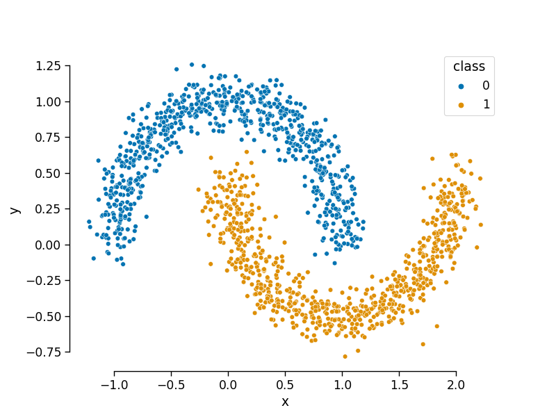
(a) Original Data

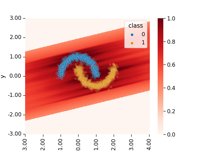
(b) OOD Detection using quantile representations

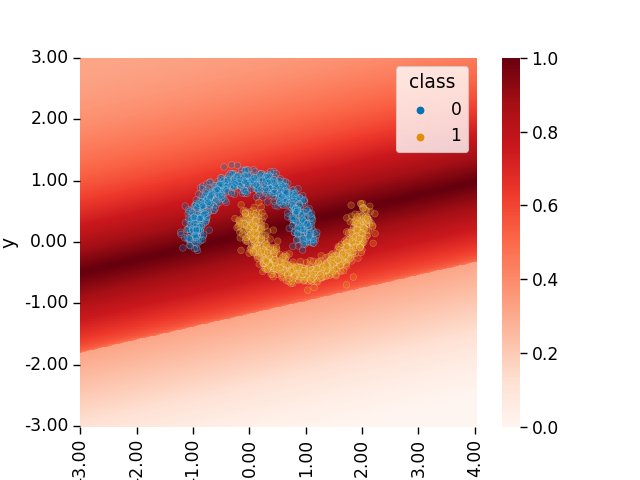
(c) OOD Detection using Probabilities

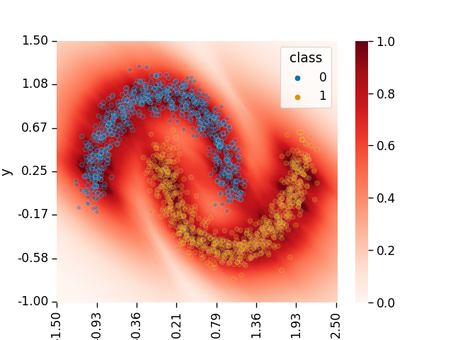
(d) Using Random Labels

Figure 5: Illustrating a case where quantile representations do not capture the distribution perfectly. (a) Original Dataset. (b) The region detected as in-distribution by using quantile representations. (c) Region detected as in-distribution by using the outputs from a single classifier. Observe that quantile representations still perform better than single classifier outputs. (d) Using random labels instead of ground-truth. Observe that the two moons structure is faithfully preserved in this image. The brightness of Red indicates the chance of being in-distribution.

In figure 5 we illustrate an example where quantile representations do not capture the entire distribution. Here we use the same data as in figure 1, but with different class labels. This is shown in figure 5(a). When we perform the OOD detection we get the region as in figure 5(b). Observe that while it does detect points far away from the data as out-of-distribution, the moon structure is not identified. In particular, the spaces between the moons is not considered OOD. This illustrates a case when quantile representations might fail.

However, OOD detection using a single classifier also fail, as illustrated in figure 5(c). Observe that the region identified by quantile representations is much better than the one obtained using a single classifier.

A simple fix for OOD detection:

If OOD detection were the aim, then it is possible to change the approach slightly by considering random labels instead of the ground-truth labels. This allows us to identify arbitrary regions where the data is located. This is illustrated in figure 5(d). Observe that this method can be used to identify any region in the space by suitably sampling and assigning pseudo-labels. In this case, we identify the training data perfectly.

Appendix D Cannot Correct Calibration Error

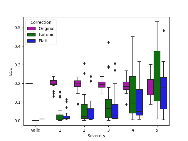
(a) Densenet

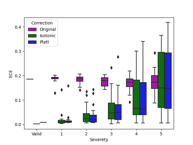
(b) Resnet

Figure 6: Correcting calibration error on the validation set may not improve performance on corrupted datasets. The figure illustrates the use of Platt scaling and Isotonic regression to correct the calibration error on the validation set, but this leads to an increase in the calibration error on the corrupted dataset. This suggests that it may not be possible to correct the calibration error simply by adjusting the probability scores.

Figure 4 shows that calibration error from quantile representations is robust to noise. So, an obvious question which follows is - Can we then correct it using validation data and improve the calibration score? It turns out that this is not possible. Remark: A similar result is also obtained in Proposition 1 of [7].

To verify this we perform the same experiment as in section 4.4. Further we use Platt Scaling and Isonotic regression on validation data and accordingly transform the probability estimates for the corrupted datasets. These results are shown in figure 6.

Surprisingly, we find that correcting for calibration on the validation set actually leads to an increase in the calibration error on corrupted datasets. It is currently unclear why this is the case. Our hypothesis is that this calibration error may be due to the insufficient modeling of the underlying distribution by $f({\bm{x}})$. For example, if the true underlying model is quadratic but we are using a linear model for classification, the calibration error caused by this mismatch cannot be corrected.

Remark: Using techniques as described in [42] can be useful to correct this, since the correction is dependent on the underlying output features and not just the probabilities.

Appendix E Matching Quantile-Representations to correct the distribution

In this part we illustrate the matching of quantile-representations to correct for distribution shifts following the ideas from [37]. Let $X$ denote the original distribution of the data, and let $\Phi(X)$ denote the modified distribution. We assume that the function $\Phi(.)$ is deterministic but unknown.

If both $X$ and $\Phi(X)$ are known, then it is easy to estimate $\Phi(.)$ using some model such as neural networks. However, in reality we do not have this information. Once the environment changes, the data collected will be very different from the original ones and we do not know how $\Phi(.)$ distorts the original data. So, the aim is to estimate $\Phi(.)$ without the knowledge of $X$ and $\Phi(X)$. This is where the fact that - quantile-representations capture the distribution information becomes relevant.

Is this even possible?

Let ${\mathcal{Q}}({\bm{x}},\tau)$ denote the quantile representation obtained using $X$, and ${\mathcal{Q}}_{\Phi}({\bm{x}},\tau)$ denote the quantile representation obtained using $\Phi(X)$. Let the data collected in the new environment be $\{\hat{{\bm{x}}}_{i}\}$, then we should have that

$$\int_{\tau=0}^{1}|{\mathcal{Q}}(\Phi^{-}(\hat{{\bm{x}}}_{i}),\tau)-{\mathcal{Q}}_{\Phi}(\hat{{\bm{x}}_{i}},\tau)|=0$$ (22)

Using this it is possible to estimate $\Phi^{-}$ and hence $\Phi$.

Observe the following - Functions ${\mathcal{Q}}(.,.)$ and ${\mathcal{Q}}_{\Phi}(.,.)$ are learnt from the data using the labels, and depends on it. So, one needs the labels to specify the directions in which distribution should be the same.

For instance, consider the following example - Assume we wish to classify the candidates as suitable/not-suitable for a job based on a set of features. Now, what is suitable/not-suitable changes with with time. As well as the ability (represented in features) of the general population. So, we collect data at time $t=t_{0}$, $\{({\bm{x}}_{i,t_{0}},y_{i,t_{0}})\}$ and at time $t=t_{1}$, $\{({\bm{x}}_{i,t_{1}},y_{i,t_{1}})\}$. However we do not know the relation between ${\bm{x}}_{i,t_{0}}$ and ${\bm{x}}_{i,t_{1}}$. In such cases, matching quantile representations can be useful.

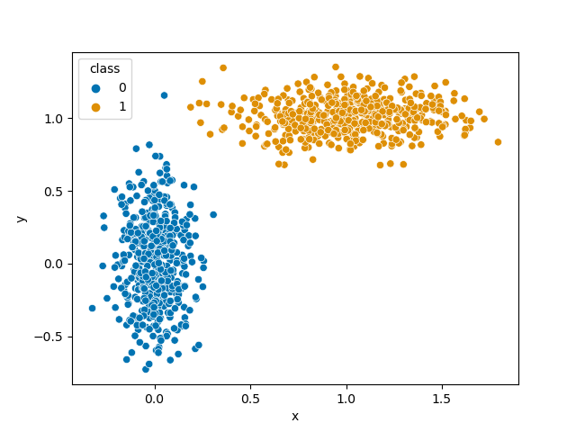
(a) Original Dataset ($X_{t_{0}}$)

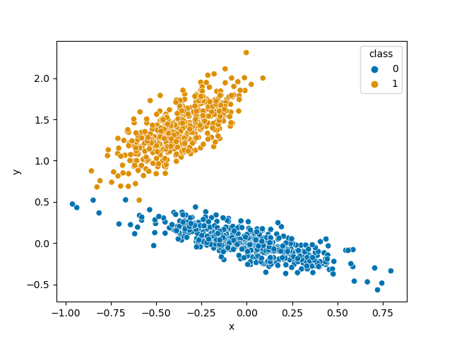
(b) Shifted Dataset ($X_{t_{1}}$)

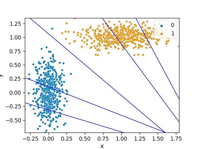
(c) Boundaries at different quantiles (Original data)

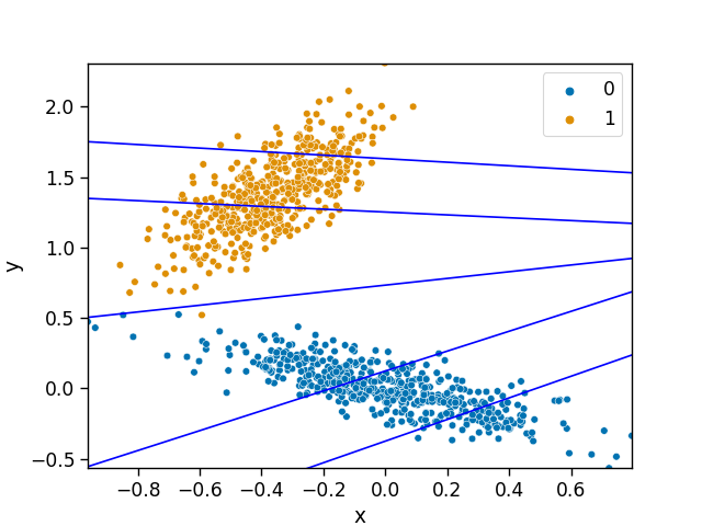
(d) Boundaries at different quantiles (Shifted data)

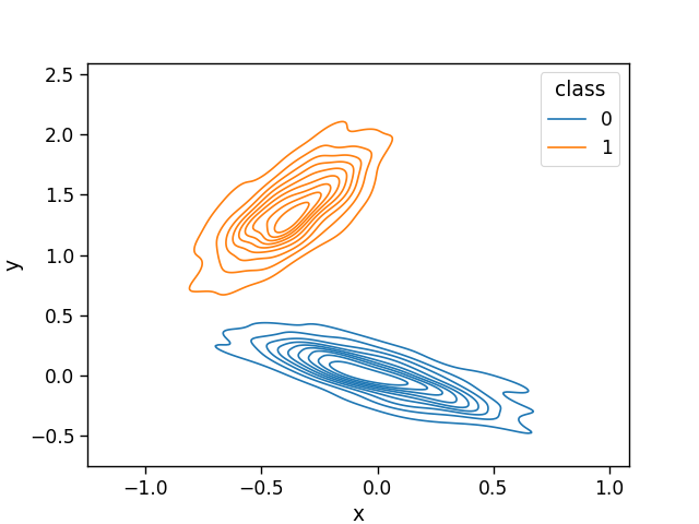
(e) Distribution of $X_{t_{1}}$

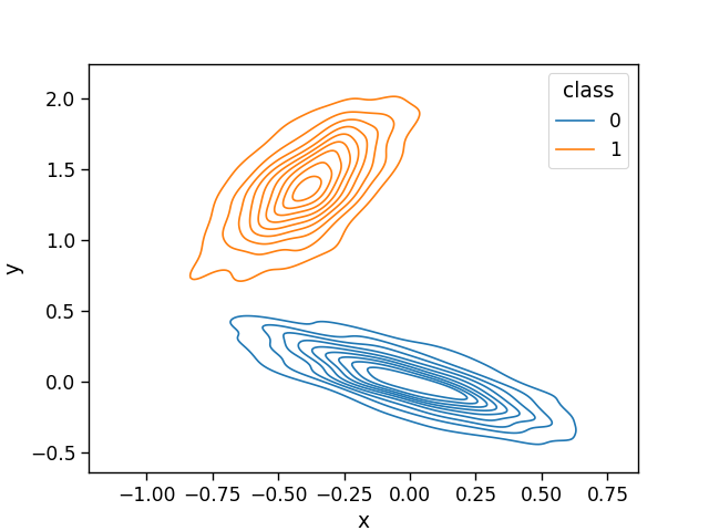
(f) Distribution of data $\Phi(X_{t_{0}})$

Figure 7: Matching quantile representations. Observe that the estimated distribution at time $t_{1}$ is similar to the actual distribution at time $t_{1}$. This shows that the estimate of $\Phi()$ is accurate.

Illustration: Matching of quantile representations

The above procedure is illustrated in figure 7. Consider the data at $t_{0}$ as in figure 7(a) and data at $t_{1}$ as in figure 7(b). This data in figure 7(a) is generated using 2d Gaussian distribution with centers $[[0,0],[1,1]]$ and standard deviation $[[0.1,0.3],[0.3,0.11]]$. We refer to this distribution as $X_{t_{0}}$. Data in figure 7(b) is obtained by generating a new sample with the same distribution as $X_{t_{0}}$ and transforming it using a random orthogonal matrix. We refer to this distribution using $X_{t_{1}}$. Note that there is no correspondence between the data samples at $X_{t_{0}}$ and $X_{t_{1}}$. Figures 7(c) and 7(d) illustrate the quantile representations obtained using the class labels at both these times. We then estimate $\Phi()$ using equation 22. Figure 7(e) shows the density at $X_{t_{1}}$ and Figure 7(f) shows the density of $\Phi(X_{t_{0}})$. Observe that the estimate of the density and the actual density match. This shows that quantile representations can be used to correct distribution shifts.

Caveat:

However, quantile-representations cannot estimate $\Phi()$ which do not change the distribution of the samples. For instance if $X_{t_{1}}=-X_{t_{0}}$, and if $X_{t_{0}}$ is symmetric around $0$, then the quantile-representations are identical. Under what conditions can $\Phi(.)$ be estimated is considered for future work.

Advantage of using quantile-representations

A question which follows is - Why not simply retrain the classifier at $t_{0}$? (i) As can be gleaned from the above experiments, it is not possible to estimate $\Phi()$ from the single classifier alone, but can be done using quantile-representations (ii) The labels considered for constructing the quantile-representations need not be the same as the classification labels. They would correspond to important attributes of the data. For instance, one can consider aspects like technical skill of the candidate instead of simply suitable/not-suitable classification.

References

- [1] Anastasios N. Angelopoulos, Stephen Bates, Emmanuel J. Candès, Michael I. Jordan, and Lihua Lei. Learn then test: Calibrating predictive algorithms to achieve risk control. arXiv preprint arXiv:2110.01052, 2021.
- [2] Jr. Bassett, Gilbert W., Roger Koenker, and Gregory Kordas. Pessimistic Portfolio Allocation and Choquet Expected Utility. Journal of Financial Econometrics, 2(4):477–492, 09 2004.
- [3] Koby Bibas, Meir Feder, and Tal Hassner. Single layer predictive normalized maximum likelihood for out-of-distribution detection. In Neural Inform. Process. Syst., 2021.
- [4] Markus M. Breunig, Hans-Peter Kriegel, Raymond T. Ng, and Jörg Sander. Lof: Identifying density-based local outliers. ACM SIGMOD Int. Conf. on Management of data, 2000.
- [5] Probal Chaudhuri. Generalized regression quantiles: Forming a useful toolkit for robust linear regression. L1 Statistical Analysis and Related Methods, Amsterdam: North-Holland, pages 169–185, 1992.
- [6] Probal Chaudhuri. On a geometric notion of quantiles for multivariate data. Journal of the American Statistical Association, 91(434):862–872, 1996.
- [7] Youngseog Chung, Willie Neiswanger, Ian Char, and Jeff Schneider. Beyond pinball loss: Quantile methods for calibrated uncertainty quantification. In Neural Inform. Process. Syst., 2021.
- [8] W. S. Cleveland. Robust Locally Weighted Regression and Smoothing Scatterplots. Journal of the American Statistical Association, 59(1):829–836, 1979.
- [9] Max H. Farrell, Tengyuan Liang, and Sanjog Misra. Deep neural networks for estimation and inference. Econometrica, 89(1):181–213, 2021.
- [10] Shai Feldman, Stephen Bates, and Yaniv Romano. Calibrated multiple-output quantile regression with representation learning. arXiv preprint arXiv:2110.00816, 2021.
- [11] Shai Feldman, Stephen Bates, and Yaniv Romano. Improving conditional coverage via orthogonal quantile regression. In Neural Inform. Process. Syst., 2021.
- [12] Stanislav Fort, Jie Ren, and Balaji Lakshminarayanan. Exploring the limits of out-of-distribution detection. In Neural Inform. Process. Syst., 2021.
- [13] Aritra Ghosh, Himanshu Kumar, and P. S. Sastry. Robust loss functions under label noise for deep neural networks. In AAAI Conf. on Artificial Intelligence, 2017.
- [14] Chuan Guo, Geoff Pleiss, Yu Sun, and Kilian Q. Weinberger. On calibration of modern neural networks. In Int. Conf. Mach. Learning, 2017.
- [15] Trevor Hastie, Robert Tibshirani, and Jerome Friedman. The Elements of Statistical Learning: Data Mining, Inference, and Prediction. Springer New York, NY, 2009.
- [16] Kaiming He, Xiangyu Zhang, Shaoqing Ren, and Jian Sun. Deep residual learning for image recognition. In Proc. Conf. Comput. Vision Pattern Recognition, 2016.
- [17] Dan Hendrycks and Thomas G. Dietterich. Benchmarking neural network robustness to common corruptions and perturbations. In Int. Conf. on Learning Representations, 2019.
- [18] Dan Hendrycks and Kevin Gimpel. A baseline for detecting misclassified and out-of-distribution examples in neural networks. In Int. Conf. on Learning Representations, 2017.
- [19] Gao Huang, Zhuang Liu, Laurens van der Maaten, and Kilian Q. Weinberger. Densely connected convolutional networks. In Proc. Conf. Comput. Vision Pattern Recognition, 2017.
- [20] Heinrich Jiang, Been Kim, Melody Y. Guan, and Maya R. Gupta. To trust or not to trust A classifier. In Neural Inform. Process. Syst., 2018.
- [21] Roger Koenker. Quantile Regression. Econometric Society Monographs. Cambridge University Press, 2005.
- [22] Gregory Kordas. Smoothed binary regression quantiles. Journal of Applied Econometrics, 21(3):387–407, 2006.
- [23] Alex Krizhevsky, Vinod Nair, and Geoffrey Hinton. The cifar-10 dataset. online: http://www. cs. toronto. edu/kriz/cifar. html, 2014.
- [24] Balaji Lakshminarayanan, Alexander Pritzel, and Charles Blundell. Simple and scalable predictive uncertainty estimation using deep ensembles. In Neural Inform. Process. Syst., 2017.
- [25] Kimin Lee, Kibok Lee, Honglak Lee, and Jinwoo Shin. A simple unified framework for detecting out-of-distribution samples and adversarial attacks. In Neural Inform. Process. Syst., 2018.
- [26] Shiyu Liang, Yixuan Li, and R. Srikant. Enhancing the reliability of out-of-distribution image detection in neural networks. In Int. Conf. on Learning Representations, 2018.
- [27] Jeremiah Z. Liu, Zi Lin, Shreyas Padhy, Dustin Tran, Tania Bedrax-Weiss, and Balaji Lakshminarayanan. Simple and principled uncertainty estimation with deterministic deep learning via distance awareness. In Neural Inform. Process. Syst., 2020.
- [28] Matthias Minderer, Josip Djolonga, Rob Romijnders, Frances Hubis, Xiaohua Zhai, Neil Houlsby, Dustin Tran, and Mario Lucic. Revisiting the calibration of modern neural networks. In Neural Inform. Process. Syst., 2021.
- [29] Yuval Netzer, Tao Wang, Adam Coates, Alessandro Bissacco, Bo Wu, and Andrew Y. Ng. Reading digits in natural images with unsupervised feature learning. In Neural Inform. Process. Syst. Workshops, 2011.
- [30] Anh Mai Nguyen, Jason Yosinski, and Jeff Clune. Deep neural networks are easily fooled: High confidence predictions for unrecognizable images. In Proc. Conf. Comput. Vision Pattern Recognition, 2015.
- [31] Yaniv Ovadia, Emily Fertig, Jie Ren, Zachary Nado, David Sculley, Sebastian Nowozin, Joshua V. Dillon, Balaji Lakshminarayanan, and Jasper Snoek. Can you trust your model’s uncertainty? evaluating predictive uncertainty under dataset shift. arXiv preprint arXiv:1906.02530, 2019.
- [32] Emanuel Parzen. Quantile probability and statistical data modeling. Statistical Science, 19(4):652–662, 2004.
- [33] J. Platt. Probabilistic outputs for support vector machines and comparison to regularized likelihood methods. In Advances in Large Margin Classifiers, 2000.
- [34] Stephen Portnoy and Roger Koenker. Adaptive l-estimation for linear models. The Annals of Statistics, 17(1):362–381, 1989.
- [35] Marco Túlio Ribeiro, Sameer Singh, and Carlos Guestrin. ”why should I trust you?”: Explaining the predictions of any classifier. In Proc. ACM SIGKDD Conf. Knowledge Discovery and Data Minining, 2016.
- [36] Bernhard Schölkopf, John C. Platt, John Shawe-Taylor, Alexander J. Smola, and Robert C. Williamson. Estimating the support of a high-dimensional distribution. Neural Comput., 13(7):1443–1471, 2001.
- [37] Nikolaos Sgouropoulos, Qiwei Yao, and Claudia Yastremiz. Matching a distribution by matching quantiles estimation. Journal of the American Statistical Association, 110(510):742–759, 2015. PMID: 26692592.
- [38] Natasa Tagasovska and David Lopez-Paz. Single-model uncertainties for deep learning. In Neural Inform. Process. Syst., 2019.
- [39] Anuj Tambwekar, Anirudh Maiya, Soma S. Dhavala, and Snehanshu Saha. Estimation and applications of quantiles in deep binary classification. IEEE Trans. Artif. Intell., 3(2):275–286, 2022.
- [40] Pingmei Xu, Krista A Ehinger, Yinda Zhang, Adam Finkelstein, Sanjeev R Kulkarni, and Jianxiong Xiao. Turkergaze: Crowdsourcing saliency with webcam based eye tracking. arXiv preprint arXiv:1504.06755, 2015.
- [41] Fisher Yu, Yinda Zhang, Shuran Song, Ari Seff, and Jianxiong Xiao. Lsun: Construction of a large-scale image dataset using deep learning with humans in the loop. arXiv preprint arXiv:1506.03365, 2015.
- [42] Yaodong Yu, Stephen Bates, Yi Ma, and Michael I. Jordan. Robust calibration with multi-domain temperature scaling. arXiv preprint arXiv:2206.02757, 2022.
- [43] Bianca Zadrozny and Charles Elkan. Transforming classifier scores into accurate multiclass probability estimates. In Proc. ACM SIGKDD Conf. Knowledge Discovery and Data Minining, 2002.