TensoIR: Tensorial Inverse Rendering
Supplementary Material

Appendix A Overview

In this supplementary material, we show more results of our method, including the detailed per-scene reconstruction results of the four synthetic scenes (Sec. B) and additional reconstruction results on four complex real scenes (Sec. C). We discuss the implementation details of our method and give an analysis of our design choices and the effects of different loss weights in Sec. D. Then, in Sec. E, we give more details about our setups on synthetic dataset generation and our multi-light capture, and provide an in-depth analysis of the multi-light results. Finally, we discuss the limitations of our methods in Sec. F.

Scene	Method	Normal	Albedo			Novel View Synthesis			Relighting
Scene	Method	MAE $\downarrow$	PSNR $\uparrow$	SSIM $\uparrow$	LPIPS $\downarrow$	PSNR $\uparrow$	SSIM $\uparrow$	LPIPS $\downarrow$	PSNR $\uparrow$	SSIM $\uparrow$	LPIPS $\downarrow$
Lego	NeRFactor	9.767	25.444	0.937	0.112	26.076	0.881	0.151	23.246	0.865	0.156
	InvRender	9.980	21.435	0.882	0.160	24.391	0.883	0.151	20.117	0.832	0.171
	Ours (25 min)	7.780	26.000	0.910	0.138	32.180	0.952	0.061	27.430	0.935	0.094
	Ours	5.980	25.240	0.900	0.145	34.700	0.968	0.037	28.581	0.944	0.081
	Ours w/ three rotated lights	5.630	25.640	0.909	0.141	34.590	0.968	0.037	28.955	0.949	0.077
	Ours w/ three general lights	5.370	25.560	0.905	0.146	34.350	0.967	0.038	29.008	0.947	0.078
Hotdog	NeRFactor	5.579	24.654	0.950	0.142	24.498	0.940	0.141	22.713	0.914	0.159
	InvRender	3.708	27.028	0.950	0.094	31.832	0.952	0.089	27.630	0.928	0.089
	Ours (25 min)	4.330	29.390	0.947	0.099	34.920	0.967	0.068	27.353	0.927	0.124
	Ours	4.050	30.370	0.947	0.093	36.820	0.976	0.045	27.927	0.933	0.115
	Ours w/ three rotated lights	3.240	30.180	0.959	0.079	35.310	0.972	0.051	28.459	0.939	0.110
	Ours w/ three general lights	3.220	31.240	0.958	0.080	35.670	0.973	0.048	28.952	0.939	0.110
Armadillo	NeRFactor	3.467	28.001	0.946	0.096	26.479	0.947	0.095	26.887	0.944	0.102
	InvRender	1.723	35.573	0.959	0.076	31.116	0.968	0.057	27.814	0.949	0.069
	Ours (25 min)	2.360	31.860	0.983	0.068	35.160	0.978	0.053	32.358	0.968	0.056
	Ours	1.950	34.360	0.989	0.059	39.050	0.986	0.039	34.504	0.975	0.045
	Ours w/ three rotated lights	1.590	34.960	0.990	0.058	38.480	0.985	0.041	34.889	0.977	0.042
	Ours w/ three general lights	1.550	34.270	0.989	0.057	38.230	0.984	0.043	34.941	0.977	0.043
Ficus	NeRFactor	6.442	22.402	0.928	0.085	21.664	0.919	0.095	20.684	0.907	0.107
	InvRender	4.884	25.335	0.942	0.072	22.131	0.934	0.057	20.330	0.895	0.073
	Ours (25 min)	5.040	25.590	0.948	0.059	27.140	0.958	0.062	23.076	0.935	0.083
	Ours	4.420	27.130	0.964	0.044	29.780	0.973	0.041	24.296	0.947	0.068
	Ours w/ three rotated lights	3.950	27.910	0.968	0.038	29.200	0.972	0.043	24.765	0.951	0.067
	Ours w/ three general lights	4.060	26.220	0.952	0.054	28.640	0.967	0.050	24.622	0.949	0.068

Table 1: Per-scene results on the synthetic datasets.

Appendix B Per-Scene Results on the Synthetic Dataset

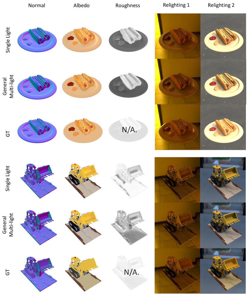
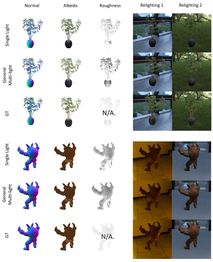
In Tab. 1, we provide the results for individual synthetic scenes mentioned in Sec. 4 of the main paper. Our method outperforms both baselines in all four scenes. Figure 6 and Fig. 7 show our recovered normal, albedo, roughness, and relighting results from both our single- and multi-light-models on the four synthetic scenes.

Appendix C Results on Real-World Captures

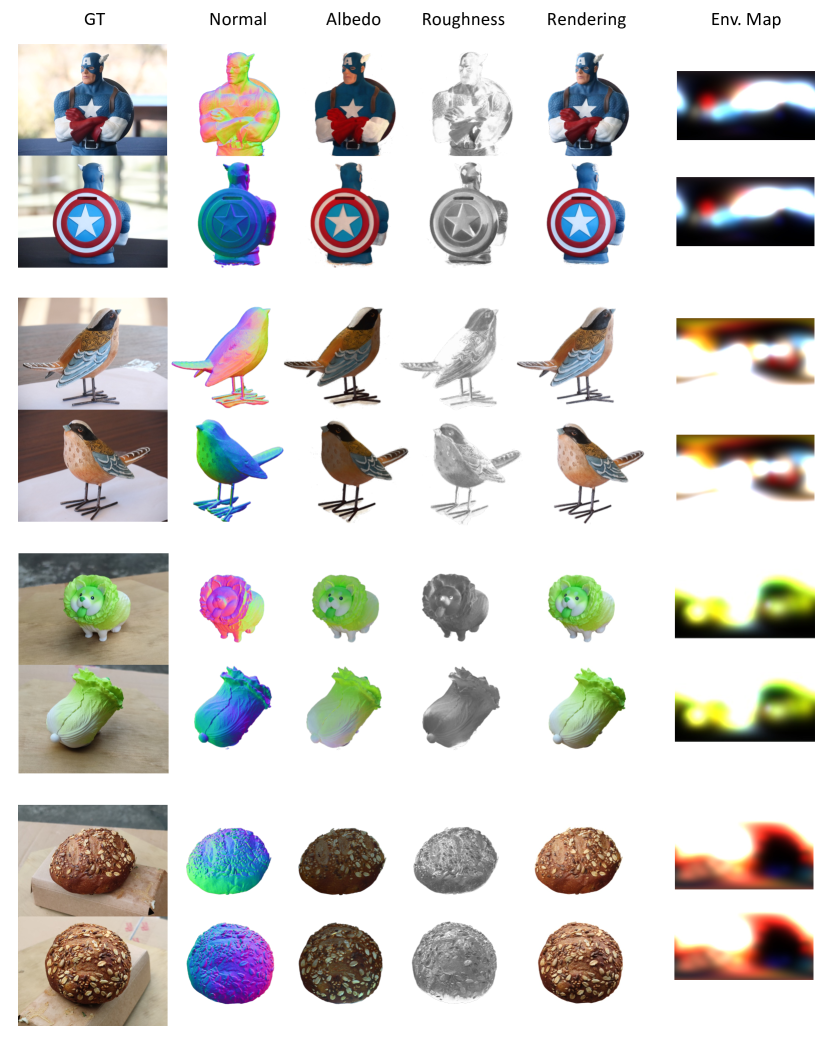
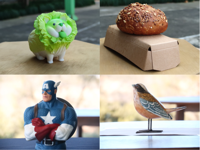
We capture 4 real objects (shown in Fig. 1) under natural illumination in the wild to evaluate our method on real data. When capturing, we fix the camera parameters (exposure time, ISO, etc) and (roughly) uniformly take photos around the object. We use commercial softwares (picwish and remove.bg) to remove the background in each photo and use COLMAP to estimate the camera poses. Figure 8 shows our reconstructed geometry, BRDF, and lighting on the real data. Note the quality of our reconstruction is affected by practical issues, such as the background removal quality, imperfect camera calibration, and non-static environment lighting (since there could be people passing by our in-the-wild setup). Nonetheless, our real-data results are still of very high quality. Please also see our video for more visual results.

Refer to caption — Figure 1: Four real objects we captured under natural lighting conditions. Please see Fig. 8 for their reconstruction results.

Appendix D Implementation Details

Representation details. As described in Sec. 3.2 in the main paper, we use a 3D density tensor $\mathcal{G}_{\sigma}$ and a 4D appearance tensor $\mathcal{G}_{a}$ in our TensoRF-based scene representation; both tensors are factorized as multiple tensor components with vector and matrix factors. As in TensoRF, our model generally works well for any spatial resolutions of the feature grids and any number of tensor components; in general, higher solutions and more components lead to better reconstruction quality. For most cases, we use a spatial resolution of $300^{3}$ ; to achieve better details on scenes with complex thin structures (like Ficus), we use a resolution of $400^{3}$ . For all results, we use 48 tensor components (16 components per dimension) for the density tensor and 144 components (48 components per dimension) for the appearance tensor separately. For decoding the multiple appearance properties, we design our MLP decoder networks all as a small two-layer MLP with 128 channels in each hidden layer and ReLU activation. In addition, the Radiance Net receives the appearance feature and viewing direction as input, and the Normal Net and BRDF Net will receive intrinsic feature and 3D location as input. Frequency encoding is applied on both directions and locations.

For our multi-light representation (in Sec. 3.4 of the paper), we leverage the mean appearance feature $\bar{a}_{\mathbf{x}}$ (Eqn. 8) for normal and reflectance decoding. In practice, this mean is computed with the means of lighting vectors $\mathbf{e}$ , averaged along the lighting dimension, without computing individual $a_{\mathbf{x},l}$ for lower costs, leveraging the linearity of Eqn. 9).

Training details. We run our model on a single RTX 2080 Ti GPU(11 GB memory) for all our results. For fair comparisons, the baseline methods (NeRFactor and InvRender) are also re-run with the same GPU to test their run-time performance. We train our full model using Adam optimizer; following TensoRF, we use initial learning rates of 0.02 and 0.001 for tensor factors and MLPs respectively. We also perform coarse-to-fine reconstruction as done in TensoRF by linearly upsampling our spatial tensor factors (started from $N^{3}_{0}$ = $128^{3}$ for all cases) multiple times during reconstruction until achieving the final spatial resolution ( $N^{3}$ = $300^{3}$ in most cases as mentioned). We upsample the vectors and matrices linearly and bilinearly at steps 10000, 20000, 30000, 40000 with the numbers of voxels interpolated between $N^{3}_{0}$ and $N^{3}$ linearly in logarithmic space.

The total training iteration is 80k and the average training time is 5 hours. The first 10k will be used to generate alphaMask, which is also used in the original TensoRF, to help skip empty space, so it only has radiance field rendering to compute image loss and only costs about 5 minutes. We do so because we find the alphaMask can greatly help to reduce the GPU memory cost of physically-based rendering: We find that if we directly perform physically-based rendering directly at the very beginning of the training process without generating the alphaMask, the training ray batch size can not be larger than 1024, otherwise, we would meet cuda-out-of-memory errors. And because we spend a few minutes generating a coarse alphaMask (which will be updated in the later training process), we can sample 4096 camera rays for each training batch. The number of points sampled per camera ray is determined by the grid resolution; a grid size of $300^{3}$ leads to about 1000 points per ray.

Ray marching details. During training, when computing the visibility and indirect lighting, we sample 512 secondary rays starting from each surface point with 96 points per ray, and half of the rays will be filtered according to surface normal orientation (only those rays whose directions lie in the upper hemisphere of the normal vector will be valid). The sampled rays’ directions are generated by stratified sampling (We divide the environmental map into grids with equal 2D areas and generate a random direction inside each grid). Also, the visibility gradients and indirect lighting gradients are detached for GPU memory consideration. While our secondary ray sample is coarser than primary (camera) ray sampling, we find this is enough to achieve accurate shadowing and indirect lighting computation.

During relighting, since we have testing ground-truth environmental maps as input, we use lighting-intensity importance sampling during ray sampling instead of stratified sampling, which means we will sample more rays near those directions that have stronger lighting.

Loss details. Our model is reconstructed with a combination of multiple loss terms as introduced in Sec. 3.5 and Eqn. 13 in the paper. We now introduce the details of the BRDF smoothness term $\ell_{\boldsymbol{\beta}}$ and normal back-facing term $\ell_{\mathbf{d}}$ in Eqn. 13. In particular, we impose scale-invariant smoothness terms on our BRDF predictions (both roughness and albedo) to encourage their spatial coherence. For each sample point on the camera ray, we minimize the relative difference of its predicted material properties from those of the randomly-sampled neighboring points, defined as:

\ell_{\boldsymbol{\beta}}=\sum_{j,\ \mathbf{x}=\mathbf{r}(t_{j})}w_{j}\left\|\frac{\boldsymbol{\beta}_{\mathbf{x}}-\boldsymbol{\beta}_{\mathbf{x}+\boldsymbol{\xi}}}{\mathbf{max}(\boldsymbol{\beta}_{\mathbf{x}},\boldsymbol{\beta}_{\mathbf{x}+\boldsymbol{\xi}})}\right\|_{2}^{2}

(1)

where $\boldsymbol{\xi}$ is a small random translation vector generated from a normal distribution with zero mean and 0.01 variance, and $w_{j}$ is the volume rendering weights (as described in Eqn. 2 in the paper) to assign large weights for points around the object surface. This weight $w_{j}$ has also been used for other loss terms (including the normal regularization term $\ell_{\mathbf{n}}$ in Eqn. 12). In addition, we also regularize the predicted normals by penalizing those that are near the surface and back-facing with the orientation loss introduced by Ref-NeRF:

\ell_{\mathbf{d}}=\sum_{j}w_{j}\max(0,\mathbf{n}_{j}\cdot\mathbf{d})

(2)

We also have a TV loss shortly in the process of generating alphaMask to help eliminate some small floaters.

We set the radiance field rendering loss weight $\alpha_{\text{RF}}$ to be 1.0, physically-based rendering loss weight $\alpha_{\text{PB}}$ to be 0.2, and BRDF smoothness regulation loss weight to be 0.001. The $\ell_{1}$ -regularization on all tensor factors has the same loss weight as TensoRF. The weight $\alpha_{\mathbf{n}}$ for normals difference loss $\ell_{\mathbf{n}}$ (the loss that constrains the difference between the predicted normals from Normal Net and the derived normals from the density field) is crucial for the final reconstruction quality. We find reasonable weights to lie in $\left[4\times 10^{-4},6\times 10^{-3}\right]$ . Larger normals difference loss $\alpha_{\mathbf{n}}$ can help to prevent the Normal Net prediction from overfitting on input images but will at the same time damage the network’s ability to predict high-frequency details.

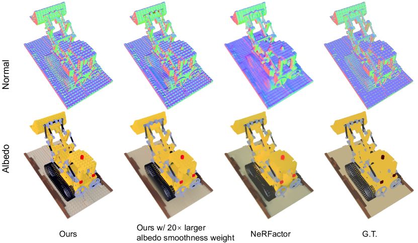
Effects of BRDF smoothness loss on lego’s reconstruction. We give more analysis and explanations about the artifacts of our albedo reconstruction result on lego scene, which has been discussed partly in the main paper. As shown by Fig. 5 of the main paper, NeRFactor’s albedo result on the lego scene looks closer to the ground truth than our results because its result looks smoother. In the main paper, we claim that this is because that NeRFactor uses a high-weight BRDF smoothness loss, which helps it achieve smooth albedo reconstruction but damages its reconstruction quality of other components. As shown in Fig. 3, when making the loss weight of our albedo smoothness loss become 20 times larger, our albedo result will be smoother and closer to the ground truth, but this will damage our normal reconstruction quality (but still better than the results of our baselines). Therefore, to have better geometry reconstruction results and to make the loss weight of BRDF smoothness loss fixed across different scenes, we do not use extra larger BRDF smoothness loss weight for lego in our experiments.

Appendix E More Details and Analysis on Our Synthetic Dataset and Multi-Light Capture

More details about our synthetic dataset and multi-light settings. we perform experiments on four complex synthetic scenes, including three blender scenes (ficus, lego, and hotdog) from the original NeRF and one (armadillo) from the Stanford 3D scanning repository. All data are re-rendered by multiple high-resolution ( $2048\times 1024$ ) environment maps to obtain their ground-truth images ( $800\times 800$ resolution) for training and testing, as well as BRDF parameters and normal maps. We use the same camera settings as NeRFactor, so we have 100 training views and 200 test views.

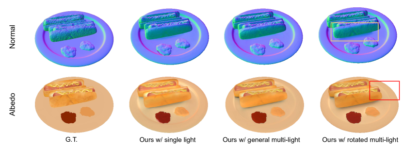
In the main paper, we discussed our results on two types of multi-light data: rotated multi-light data and general multi-light data. Rotated multi-light data is rendered under a rotated multi-light setting, in which the images are rendered from the same 100 views as in the single-light setting, but each view has 3 images rendered by rotated environment maps. we rotate the same environment map along the azimuth for 0, 120, and 240 degrees, which can be done in practice by rotating the captured object (as done in Fig. 4). And with known rotation degrees, our method can optimize shared environmental lighting across the rotated multi-light data. General multi-light data is rendered under a general multi-light setting, in which we create three lighting conditions by rendering the objects with three unrelated environment maps, which will be optimized separately in the later training process.

Considering both multi-light settings above have more input training images than the single-light setting (the number of training views is the same, but multi-light settings above have more images per view), we introduce the third the multi-light setting here which is called limited general multi-light setting to evaluate whether the improvements of reconstruction quality under multi-light setting are due to the extra number of input images. It uses the same kind of data as the general multi-light setting, but for each view we will only randomly select one image as training input from the 3 images under different lighting conditions, which guarantees that the number of training images in this setting is the same as the single-light setting. As shown in Tab. 2, while using the same number of images, such a setting still achieves better performance in BRDF estimation and geometry reconstruction than the single-light setting, which demonstrates the benefits of the multi-light input.

Method	Normal MAE $\downarrow$	Albedo PSNR $\uparrow$	NVS PSNR $\uparrow$
Ours w/ single-light	4.100	29.275	35.258
Ours w/ rotated multi-light	3.602	29.672	34.395
Ours w/ general multi-light	3.551	29.326	34.395
Ours w/ limited general multi-light	3.670	29.320	34.100

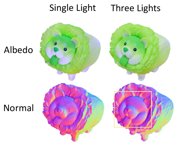
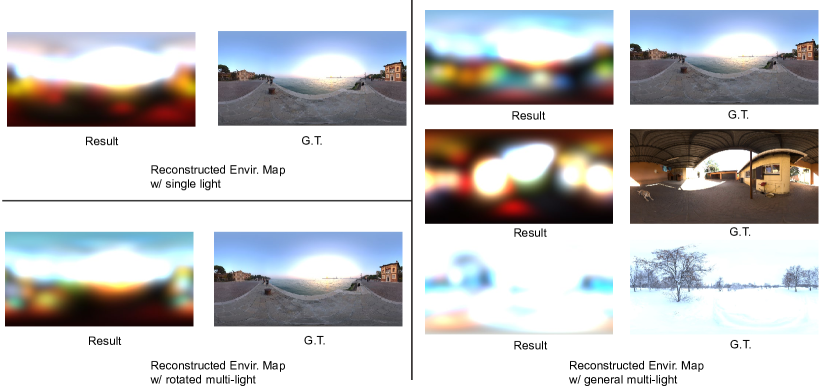
Table 2: Quantitative comparisons of results on the synthetic dataset using single-light and multi-light input.

Analysis of results with multi-light captures. As shown in Tab. 1 (and also the main paper’s Tab. 1), our approach enables effective and efficient multi-light reconstruction, leading to better reconstruction accuracy. While the single-light novel view synthesis (physically-based rendering) results are slightly better than our multi-light results, this is simply because we evaluate novel view synthesis under the same single lighting, which the single-light model is specifically trained on (and easier to overfit). On the other hand, our multi-light model achieves better reconstruction and leads to much better rendering quality under novel lighting conditions (as shown by the relighting results). We also show visual comparisons between our single-light and multi-light results on both synthetic and real scenes in Fig. 2 and Fig. 4. Our multi-light reconstruction recovers more details in the normal maps and recovers better shading- and artifact-free albedo maps. We also achieve rotated multi-light capture for the real data by simply rotating the object three times. Our results in Fig. 4 show that even such simple multi-light acquisition can already lead to high-quality reconstruction in practice (better than the single-light results), demonstrating the effectiveness of our multi-light reconstruction model. We also find that multi-light settings can help to solve the color ambiguity between environmental lighting and object materials. As shown by Fig. 5, the color of reconstructed environment map is closer to the ground truth under multi-light settings.

Appendix F Limitations

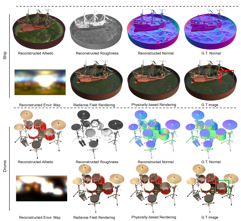
We evaluate our method on complex scenes from the original NeRF-Synthetic dataset to help understand the limitations of our method. In general, our approach has the following limitations: first, our physically-based rendering applies a surface-based rendering model, which means that we can not handle complex materials that can not be well modeled by this model, for example, translucent water that has strong reflection and refraction (see the red frame in Fig. 9) and transparent glass (see the green frame in Fig. 9). Second, we assume the materials of the objects to be dielectric (non-conducting) and therefore fix the ${F_{0}}$ in the fresnel term of our simplified Disney BRDF to be 0.04, which means in theory, we can not well model non-dielectric materials like metals. Replacing the pure physically-based BRDF with a learning-based neural BRDF that has learned data prior about materials from training data can help overcome this limitation. We leave it to be future works.