Functional Causal Inference with Time-to-Event Data

Abstract

In this Supplement, Section 1 outlines the proofs of propositions mentioned in the main paper. Section 2 presents complete algorithms for the functional causal survival framework, including FAFT estimation, regression adjustment approach, FIPW approach, and double robust approach. The additional simulation results based on a different sample size are incorporated in Section 3. Section 4 includes all causal estimators of the hippocampus in the ADNI study, which are estimated under the proposed causal framework.

1 Proofs

1.1 Proof of Proposition 1

$$\mathbb{E}\Bigl{[}\mathrm{w}Y|X\Bigr{]} =\mathbb{E}_{\mathbf{Z}}\Bigl{[}\mathbb{E}_{x,\mathbf{Z}}\left[\mathrm{w}Y|X,\mathbf{Z}\right]\Bigr{]}$$

$$=\int\mathbf{Z}\ \mathbb{E}_{x,\mathbf{Z}}\left[\mathrm{w}Y|X,\mathbf{Z}\right]f(\mathbf{Z})\mathrm{\leavevmode\nobreak\ d}\mathbf{Z}$$

$$=\int\mathbf{Z}\left[\int\frac{f(\mathbf{Z})}{f(\mathbf{Z}|X)}Yf(Y|X,\mathbf{Z})\mathrm{\leavevmode\nobreak\ d}Y\right]f(\mathbf{Z})\mathrm{\leavevmode\nobreak\ d}\mathbf{Z}$$

$$=\int\mathbf{Z}\int\frac{f(\mathbf{Z})}{f(\mathbf{Z}|X)}\frac{f(Y,\mathbf{Z}|X)}{f(\mathbf{Z})}\times Y\times f(\mathbf{Z})\mathrm{\leavevmode\nobreak\ d}Y\mathrm{\leavevmode\nobreak\ d}\mathbf{Z}$$

$$=\int\int\frac{f(\mathbf{Z})}{f(\mathbf{Z}|X)}\frac{f(Y|\mathbf{Z},X)f(\mathbf{Z}|X)}{f(\mathbf{Z})}\times\mathbf{Z}\times Y\times f(\mathbf{Z})\mathrm{\leavevmode\nobreak\ d}Y\mathrm{\leavevmode\nobreak\ d}\mathbf{Z}$$

$$=\int\int Y\times f(Y|\mathbf{Z},X)\mathrm{\leavevmode\nobreak\ d}Y\times\mathbf{Z}\times f(\mathbf{Z})\mathrm{\leavevmode\nobreak\ d}\mathbf{Z}$$

$$=\int_{\mathbf{Z}}\mathbb{E}\left[Y(x)|\mathbf{Z}=\mathbf{z}\right]\mathrm{\leavevmode\nobreak\ d}f_{\mathbf{Z}}(\mathbf{z})$$

$$=\int_{\mathbf{Z}}\mathbb{E}\left[Y|X=x,\mathbf{Z}=\mathbf{z}\right]\mathrm{\leavevmode\nobreak\ d}f_{\mathbf{Z}}(\mathbf{z})$$

$$=\mathbb{E}[Y(x)]$$

1.2 Proof of Proposition 2

$$\mathrm{w}\overset{\triangle}{=}\frac{f(\mathbf{Z})}{f(\mathbf{Z}|X)}\approx\frac{f(\mathbf{Z})}{f(\mathbf{Z}|\mathbf{A})}=\frac{f(\mathbf{Z})}{f(\mathbf{A}|\mathbf{Z})f(\mathbf{Z})/f(\mathbf{A})}=\frac{f(\mathbf{A})}{f(\mathbf{A}|\mathbf{Z})}\overset{\triangle}{=}w$$

2 Algorithms

2.1 Algorithm 1: FAFT estimation

Equations included in this section correspond to the main paper.

Input: $\left\{\{X_{i}(s_{1m}),1\leqslant m\leqslant M\},\mathbf{Z}_{i},\delta_{i},\widetilde{T}_{i}\ \mid\ i=1,...,n\right\}$

1. Do FPCA based on pre-determined PVE and return FPCS matrix $\left[\hat{A}_{ik}\right]_{n\times K_{n}}$ and corresponding eigenfunctions $\{\hat{\phi}_{k}(\cdot):1\leqslant k\leqslant K_{n}\}$.

2. Evaluate conditional expectations for censored subjects using Equation (10).

3. Calculate pseudo outcome $Y_{i}^{*}$ for each individual based on Equation (9).

4. Given an initial value $\hat{\boldsymbol{\theta}}^{(0)}$, at the $m$-th interation, update $\hat{\boldsymbol{\theta}}^{(m)}_{n}=L_{n}\left(\hat{\boldsymbol{\theta}}^{(m-1)}_{n}\right)$ based on Equation (11).

5. Repeat Step.4 until predetermined converging criteria is satisfied or maximum interation is reached.

6. Recover $\hat{\beta}(\cdot)$ using estimated $\{\hat{\beta}_{k},\hat{\phi}_{k}(\cdot):1\leqslant k\leqslant K_{n}\}$.

Output: $\left(\hat{\alpha},\hat{\beta}(\cdot),\hat{\gamma}_{1},...,\hat{\gamma}_{p}\right)$

2.2 Algorithm 2: Regression adjustment approach

Equations included in this section correspond to the main paper.

Input: $\left\{\{X_{i}(s_{1m}),1\leqslant m\leqslant M\},\mathbf{Z}_{i},\delta_{i},\widetilde{T}_{i}\ \mid\ i=1,...,n\right\}$

1. Fit FAFT using Algorithm 1.

2. Construct $n$ adjusted responses based on Equation 3.2 and return $\widehat{\mathbf{{Y}}}=\left(\widehat{Y}_{1},...,\widehat{Y}_{n}\right)$

3. Fit FAFT model with $\mathbf{\widehat{Y}}$ using Algorithm 1.

4. Recover $\hat{\beta}_{\text{RegAdj}}(\cdot)$.

Output: $\hat{\beta}_{\text{RegAdj}}(\cdot)$

2.3 Algorithm 3: FIPW approach

Equations included in this section correspond to this section, not the main paper.

Ideally, the functional weights are expected to achieve the balance condition for each observed individual, i.e.,

$$\mathbb{E}\left(w_{i}^{*}\mathbf{A}_{i}^{*}\mathbf{Z}_{i}^{*\top}\right)=0,\quad i=1,...,n.$$ (1)

To satisfy it, $w_{i}$ can be viewed as a minimizer of the left side of the Equation 1. According to 2021_Xiaoke, the weights can be calculated parametrically or non-parametrically. The parametric estimation assumes that $f\left(\mathbf{A}^{*}\right)\sim N(0,1)$ and $f\left(\mathbf{A}^{*}\mid\mathbf{Z}_{i}^{*}\right)\sim N(\boldsymbol{\xi}^{\top}\mathbf{Z}_{i}^{*},\boldsymbol{\Sigma}_{\mathbf{A}_{i}^{*}})$ and unknown parameters $\boldsymbol{\xi}$ and $\Sigma_{A^{*}}$ can be estimated by solving the following equations:

$$\left\{\begin{array}[]{l}n^{-1}\sum_{i=1}^{n}\left(\mathbf{A}_{i}^{*}-\boldsymbol{\xi}^{\top}\mathbf{Z}_{i}^{*}\right)\left(\mathbf{A}_{i}^{*}-\boldsymbol{\xi}^{\top}\mathbf{Z}_{i}^{*}\right)^{\top}=\boldsymbol{\Sigma}_{\mathbf{A}_{i}^{*}};\\ n^{-1}\sum_{i=1}^{n}\operatorname{det}(\boldsymbol{\Sigma}_{\mathbf{A}_{i}^{*}})^{1/2}\exp\left\{\frac{1}{2}\left(\mathbf{A}_{i}^{*}-\boldsymbol{\xi}^{\top}\mathbf{Z}_{i}^{*}\right)^{\top}\boldsymbol{\Sigma}_{\mathbf{A}_{i}^{*}}^{-1}\left(\mathbf{A}_{i}^{*}-\boldsymbol{\xi}^{\top}\mathbf{Z}_{i}^{*}\right)-\frac{1}{2}\left(\mathbf{A}_{i}^{*}\right)^{\top}\left(\mathbf{A}_{i}^{*}\right)\right\}\mathbf{A}_{i}^{*}\left(\mathbf{Z}_{i}^{*}\right)^{\top}=\mathbf{0}.\end{array}\right.$$ (2)

With estimates $\widehat{\boldsymbol{\xi}}$ and $\widehat{\boldsymbol{\Sigma}}_{\mathbf{A}_{i}^{*}}$, it’s very straightforward to calculate individual weights

$$w_{i}^{*}=\operatorname{det}(\boldsymbol{\Sigma}_{\mathbf{A}_{i}^{*}})^{1/2}\exp\left\{\frac{1}{2}\left(\mathbf{A}_{i}^{*}-\boldsymbol{\xi}^{\top}\mathbf{Z}_{i}^{*}\right)^{\top}\boldsymbol{\Sigma}_{\mathbf{A}_{i}^{*}}^{-1}\left(\mathbf{A}_{i}^{*}-\boldsymbol{\xi}^{\top}\mathbf{Z}_{i}^{*}\right)-\frac{1}{2}\left(\mathbf{A}_{i}^{*}\right)^{\top}\left(\mathbf{A}_{i}^{*}\right)\right\}.$$

The non-parametric calculation avoids the possible misspecification for the SFPS while sacrificing some computation efficiency. Equation 1) should be minimized with four restrictions shown as below:

$$E\left(w_{i}^{*}\right) =1,\quad E\left(w_{i}^{*}\mathrm{\leavevmode\nobreak\ A}_{i}^{*}\mathbf{Z}_{i}^{*\top}\right)=\mathbf{0},$$ (3)

$$E\left(w_{i}^{*}\mathbf{A}_{i}^{*}\right) =\mathbf{0},\quad E\left(w_{i}^{*}\mathbf{Z}_{i}^{*}\right)=\mathbf{0},\quad i=1,\ldots,n$$

Based on the idea of empirical likelihood method (owen2001empirical), subject to the empirical counterparts of Equation 3, the aim is to maximize $\prod_{i=1}^{n}f_{\left(\mathbf{A}^{*},\mathbf{Z}^{*}\right)}\left(\mathbf{A}_{i}^{*},\mathbf{Z}_{i}^{*}\right)$, thus leads to an equivalent optimization:

$$\min_{\mathbf{w}^{*}}\sum_{i=1}^{n}\log\left(w_{i}^{*}\right),$$

$$\text{ s.t. }\quad\sum_{i=1}^{n}w_{i}^{*}=n,\quad\sum_{i=1}^{n}w_{i}^{*}\mathbf{A}_{i}^{*}\left(\mathbf{Z}_{i}^{*}\right)^{\top}=\mathbf{0},\quad\sum_{i=1}^{n}w_{i}^{*}\mathbf{A}_{i}^{*}=\mathbf{0},\quad\sum_{i=1}^{n}w_{i}^{*}\mathbf{Z}_{i}^{*}=\mathbf{0}.$$

Due to the existence of a non-convexity issue, the regularized approach by fong2018covariate is adapted to allow an imbalance between $\mathbf{A}_{i}^{*}$ and $\mathbf{Z}_{i}^{*}$ but meanwhile penalizes such imbalance in the objective function

$$\min_{\mathbf{w}^{*},\boldsymbol{\Gamma}}\sum_{i=1}^{n}\log\left[\sum_{i=1}^{n}\log\left(w_{i}^{*}\right)+\frac{1}{2\rho}\{\operatorname{vec}(\boldsymbol{\Gamma})\}^{\top}\{\operatorname{vec}(\boldsymbol{\Gamma})\}\right],$$ (4)

$$\text{ s.t. }\quad\sum_{i=1}^{n}w_{i}^{*}=n,\quad\frac{1}{n}\sum_{i=1}^{n}w_{i}^{*}\mathbf{A}_{i}^{*}\left(\mathbf{C}_{i}^{*}\right)^{\top}=\boldsymbol{\Gamma},\quad\sum_{i=1}^{n}w_{i}^{*}\mathbf{A}_{i}^{*}=\mathbf{0},\quad\sum_{i=1}^{n}w_{i}^{*}\mathbf{Z}_{i}^{*}=\mathbf{0},$$

where $\rho>0$ is a tuning parameter and $\Gamma\text{ is a }L\times p$ matrix allowing for an imperfect balancing condition. Optimization involves the Lagrangian multiplier, profile method, and use of the Fletcher–Goldfarb–Shanno algorithm. The default value of $\rho$ is set to be $0.1/n$ suggested by fong2018covariate. More details can be found in 2021_Xiaoke. After getting $\hat{w}_{i}^{*}$ ’s, a weighted pseudo-sample created by $\boldsymbol{w}\mathbf{Y}$ will be used to fit FAFT. The following algorithm summarizes the whole procedure.

Input: $\left\{\{X_{i}(s_{1m}),1\leqslant m\leqslant M\},\mathbf{Z}_{i},\delta_{i},\widetilde{T}_{i}\ \mid\ i=1,...,n\right\}$

1. Do FPCA based on pre-determined PVE and return standardized FPCS matrix $\left[\hat{A}^{*}_{ik}\right]_{n\times K_{n}}$.

2. Calculate standardized weights $\hat{w}_{i}$ by solving Equation 2 parametrically or Equation 4 nonparametrically

3. Fit FAFT model using Algorithm 1 with created pseudo-sample

   $$\left\{\hat{w}_{i},\widetilde{T}_{i}=\min(T_{i},C_{i}),\delta_{i},X_{i}(s),\mathbf{Z}_{i}|i=1,...,n\right\}.$$

4. Recover $\hat{\beta}_{\text{FIPW}}(\cdot)$.

Output: $\hat{\beta}_{\text{FIPW}}(\cdot)$

2.4 Algorithm 4: double robust approach

Equations included in this section correspond to the main paper.

Input: $\left\{\{X_{i}(s_{1m}),1\leqslant m\leqslant M\},\mathbf{Z}_{i},\delta_{i},\widetilde{T}_{i}\ \mid\ i=1,...,n\right\}$

1. Calculate fitted adjustment responses $\left\{\hat{Y}_{\text{RegAdj},1},...,\hat{Y}_{\text{RegAdj},n}\right\}$ using Algorithm 2.

2. Calculate weights $\left\{w_{1}^{*},...,w_{n}^{*}\right\}$ using Algorithm 3.

3. Construct pseudo outcomes adjusted by weighted residuals $\left\{\widetilde{Y}_{\text{RegAdj},1},...,\widetilde{Y}_{\text{RegAdj},n}\right\}$ based on Equation (8).

4. Fit FAFT model using Algorithm 1.

5. Recover $\hat{\beta}_{\text{DR}}(\cdot)$.

Output: $\hat{\beta}_{\text{DR}}(\cdot)$

3 Additional simulation results

In this section, we report the finite sample performance of our method based on sample size $N=200$, as censoring rate varies from 20% to 60%. Figure 1 vitalizes different functional causal estimates. Table 1 summarizes all results of estimation accuracy for $\beta(\cdot)$. Table 2 summarizes all results of causal prediction accuracy for the survival outcome $Y$.

4 Additional Real Data Results

We present all causal estimators in Figure 2. The first row includes four estimators obtained via FIPW approach, and the weights are estimated parametrically, or non-parametrically with three different tuning parameter values. They are denoted as FIPW.para, FIPW.np.0 ($\rho_{0}=0.1/n$), FIPW.np.1 ($\rho_{1}=1/n$), FIPW.np.0 ($\rho_{2}=0.01/n$), respectively. In the second row, the double robust approach provides two estimators, DR.para (parametrically estimated weights) and DR.np.0 (non-parametrically estimated weights with $\rho_{0}=0.1/n$). The ’RegADj’ represents the estimator using the regression adjustment approach. For comparison, the naive estimator is also included, which assumes there is no confounding effect.

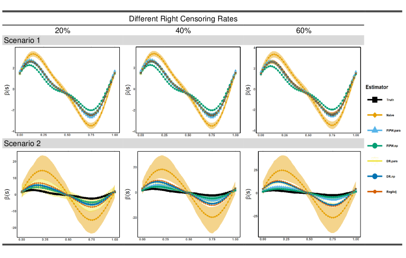
Figure 1: Plot of estimated functional causal effect curve under two scenarios with three censoring rates when sample size N=200. Different estimators are represented by line color and point shape with shading area as corresponding CI.

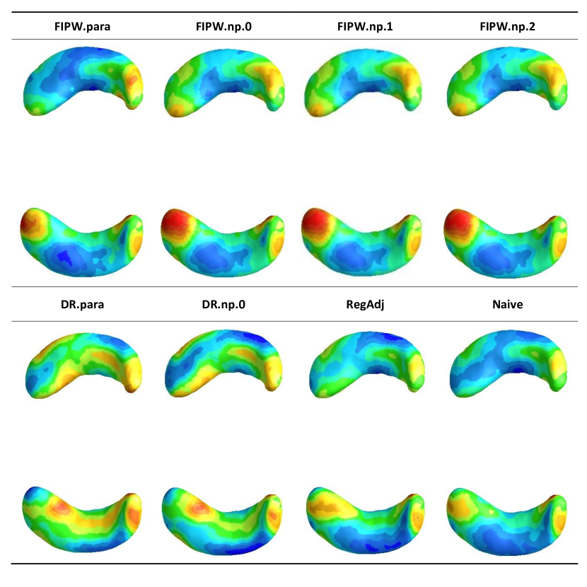
Figure 2: ADNI Data Analysis Results Using Different Estimators

Table 1: Simulation results of estimation accuracy for the functional causal curve $\beta(\cdot)$ under two scenarios with three censoring rates when sample size being $N=200$.

Different right censoring rates 20% 40% 60% RMSE AISE (SE) MISE ISB RMSE AISE (SE) MISE ISB RMSE AISE (SE) MISE ISB Scenario 1 Naive 0.18 0.51(0.058) 0.51 0.49 0.18 0.51(0.064) 0.51 0.49 0.18 0.52(0.086) 0.52 0.49 RegAdj 0.00 0.01(0.004) 0.00 0.00 0.00 0.01(0.004) 0.01 0.00 0.00 0.01(0.007) 0.01 0.00 FIPW.para 0.01 0.25(0.340) 0.15 0.03 0.01 0.28(0.407) 0.16 0.02 0.00 0.38(0.585) 0.23 0.01 FIPW.np 0.03 0.17(0.141) 0.14 0.07 0.04 0.23(0.165) 0.19 0.11 0.05 0.29(0.214) 0.25 0.12 DR.para 0.00 0.01(0.005) 0.01 0.00 0.00 0.01(0.005) 0.01 0.00 0.00 0.01(0.007) 0.01 0.00 DR.np 0.00 0.01(0.004) 0.01 0.00 0.00 0.01(0.005) 0.01 0.00 0.00 0.01(0.007) 0.01 0.00 Scenario 2 Naive 29.31 88.42(46.197) 77.78 80.31 50.06 151.70(85.456) 132.25 137.17 97.51 296.14(171.799) 254.00 267.19 RegAdj 4.38 17.14(16.232) 12.93 12.00 9.94 35.65(30.804) 27.43 27.23 22.63 78.25(66.232) 60.60 62.00 FIPW.para 2.53 7.89(3.944) 7.07 6.94 2.98 9.69(6.810) 8.24 8.16 4.14 14.46(14.887) 10.96 11.34 FIPW.np 0.89 2.96(2.115) 2.33 2.44 1.00 3.36(2.555) 2.61 2.73 0.91 3.49(3.476) 2.32 2.49 DR.para 1.71 7.94(8.262) 5.76 4.68 5.82 22.70(20.494) 16.74 15.94 15.73 58.93(53.792) 44.70 43.11 DR.np 2.18 8.25(9.997) 5.86 5.98 6.80 24.34(23.151) 18.28 18.64 17.96 64.10(57.137) 48.63 49.20

Table 2: Simulation results of prediction accuracy in terms of Root-MSE for the survival outcome $Y=\log T$ under two scenarios, both in-sample and out-sample, and with three censoring rates when sample size being $N=200$.

Different right censoring rates 20% 40% 60% Mean $q_{.25}$ $q_{.50}$ $q_{.75}$ Mean $q_{.25}$ $q_{.50}$ $q_{.75}$ Mean $q_{.25}$ $q_{.50}$ $q_{.75}$ Scenario 1 In sample Naive 2.08 1.98 2.06 2.17 2.08 1.97 2.07 2.18 2.09 1.97 2.07 2.21 RegAdj 0.53 0.50 0.53 0.56 0.54 0.50 0.53 0.57 0.55 0.51 0.55 0.59 FIPW.para 1.35 0.94 1.22 1.53 1.48 1.02 1.28 1.74 1.92 1.29 1.66 2.20 FIPW.np 1.25 1.01 1.25 1.46 1.41 1.14 1.41 1.67 1.67 1.36 1.63 1.94 DR.para 0.54 0.51 0.53 0.57 0.55 0.51 0.54 0.58 0.56 0.52 0.55 0.59 DR.np 0.54 0.50 0.53 0.57 0.54 0.51 0.54 0.58 0.56 0.52 0.55 0.59 Out sample Naive 2.03 1.85 2.03 2.20 2.03 1.86 2.03 2.21 2.04 1.84 2.03 2.23 RegAdj 0.55 0.49 0.54 0.59 0.56 0.50 0.54 0.60 0.57 0.51 0.56 0.62 FIPW.para 1.37 0.94 1.24 1.59 1.51 1.02 1.33 1.82 1.94 1.31 1.66 2.27 FIPW.np 1.27 1.02 1.24 1.51 1.44 1.14 1.42 1.70 1.68 1.33 1.61 1.96 DR.para 0.56 0.50 0.55 0.60 0.56 0.51 0.55 0.61 0.57 0.51 0.56 0.62 DR.np 0.55 0.50 0.55 0.60 0.56 0.50 0.55 0.61 0.57 0.51 0.56 0.62 Scenario 2 In sample Naive 25.91 20.79 24.76 29.82 34.75 26.92 32.80 41.22 53.31 40.10 50.56 63.61 RegAdj 10.59 7.59 9.84 12.82 18.10 13.05 16.75 21.40 35.31 25.77 33.07 41.68 FIPW.para 7.83 6.52 7.58 8.94 8.58 6.75 8.31 9.89 10.76 7.54 10.01 12.87 FIPW.np 4.71 3.46 4.42 5.77 4.98 3.69 4.65 6.09 4.81 3.05 4.25 6.08 DR.para 7.21 4.94 6.64 8.74 14.65 10.56 13.49 17.37 29.78 21.35 27.39 35.37 DR.np 7.38 4.93 6.76 9.08 14.63 10.38 13.51 17.37 29.82 21.45 27.68 35.51 Out sample Naive 25.46 20.38 24.57 29.29 34.36 26.60 33.00 40.44 53.01 39.86 50.25 62.31 RegAdj 10.35 7.33 9.75 12.48 17.99 13.00 16.57 21.56 35.34 25.37 32.94 42.39 FIPW.para 7.66 6.37 7.36 8.70 8.44 6.72 8.05 9.73 10.67 7.65 9.76 12.49 FIPW.np 4.60 3.39 4.34 5.63 4.87 3.59 4.53 5.85 4.71 2.97 4.16 5.88 DR.para 7.12 4.86 6.63 8.68 14.61 10.68 13.35 17.47 29.79 21.44 27.85 35.79 DR.np 7.22 4.92 6.74 8.99 14.53 10.29 13.34 17.50 29.79 21.27 27.78 35.66