Time-Asymmetric Fluctuation Theorem and Efficient Free Energy Estimation

Abstract

The free-energy difference $\Delta F$ between two high-dimensional systems is notoriously difficult to compute, but very important for many applications such as drug discovery  Cournia et al. (2017). We demonstrate that an unconventional definition of work introduced by Vaikuntanathan and Jarzynski (2008) satisfies a microscopic fluctuation theorem that relates path ensembles that are driven by protocols unequal under time-reversal. It has been shown before that counterdiabatic protocols—those having additional forcing that enforces the system to remain in instantaneous equilibrium, also known as escorted dynamics or engineered swift equilibration—yield zero-variance work measurements for this definition. We show that this time-asymmetric microscopic fluctuation theorem can be exploited for efficient free energy estimation by developing a simple (i.e., neural-network free) and efficient adaptive time-asymmetric protocol optimization algorithm that yields $\Delta F$ estimates that are orders of magnitude lower in mean squared error than the generic linear interpolation protocol with which it is initialized.

I Introduction

Free energy differences $\Delta F=F_{B}-F_{A}$ between pairs of potential energy functions $U_{A}({{x}})$ and $U_{B}({{x}})$ are sought after by physicists, chemists, and pharmaceutical scientists alike Cournia et al. (2017); Tawa et al. (1998); Kelly et al. (2006); Chipot and Pohorille (2007); Shirts et al. (2010); Cournia et al. (2021). Here, ${{x}}\in\mathbb{R}^{d}$ is the configuration space coordinate, and the free energy for each potential is defined as $F_{A,B}=-\beta^{-1}\ln\int e^{-\beta U_{A,B}({{x}})}\mathrm{d}{{x}}$, where $\beta=(k_{\mathrm{B}}T)^{-1}$ is inverse temperature. For high dimensional systems, $\Delta F$ can only be calculated numerically through sampling methods, which can be computationally costly and slow to converge Chipot and Pohorille (2007). Here we present an adaptive method that greatly reduces the variance of $\Delta F$ estimates, based on a new fluctuation theorem we derive.

One class of estimators takes work measurements as input from protocols $U({{x}},t)$ that “switch” $U({{x}},0)=U_{A}({{x}})\rightarrow U({{x}},t_{f})=U_{B}({{x}})$ in finite time $t_{f}$. Because the work, traditionally defined for a trajectory $X(t)|_{t\in[0,t_{f}]}$ tra as

$$W_{\mathrm{trad}}[X(t)]=\int_{0}^{t_{f}}\frac{\partial U}{\partial t}(X(t),t)\,\mathrm{d}t$$ (1)

satisfies the Jarzynski equality

$$\langle e^{-\beta W}\rangle=e^{-\beta\Delta F},$$ (2)

the Jarzynski estimator $\widehat{\Delta F}_{\mathrm{Jar}}=-\beta^{-1}\ln\,\big{(}n_{s}^{-1}\sum_{i=1}^{n_{s}}e^{-\beta W^{i}_{\mathrm{trad}}}\big{)}$ may be applied to work measurements $\{W^{i}_{\mathrm{trad}},|i=1,..,n_{s}\}$. Unfortunately this estimator can be slow to converge, because the average is often dominated by rare events.

Estimators that use bi-directional work measurements (i.e., those that also consider $U_{B}\rightarrow U_{A}$ switching processes) generally have lower variance than uni-directional work estimators Shirts and Pande (2005). In particular, Shirts et al. in Shirts et al. (2003) showed that if forward $\{W^{i}_{F}\,|\,i=1,..,n_{s}\}$ and reverse work measurements $\{W^{i}_{R}\,|\,i=1,..,n_{s}\}$, assumed here to be equal in number for simplicity, are collected from forward and reverse protocols satisfying Crooks Fluctuation Theorem

$$\mathcal{P}_{F}(+W)=\mathcal{P}_{R}(-W)\,e^{\beta(W-\Delta F)},$$ (3)

then the Bennett acceptance ratio estimator $\widehat{\Delta F}_{\mathrm{BAR}}$ Bennett (1976), defined implicitly as the $\Delta F$ satisfying

$$\sum_{i=1}^{n_{s}}\frac{1}{1+e^{-\beta(W^{i}_{F}-\Delta F)}}-\sum_{j=1}^{n_{s}}\frac{1}{1+e^{-\beta(W^{j}_{R}+\Delta F)}}=0,$$ (4)

is the lowest-variance asymptotically-unbiased estimator. Bi-directional measurements of $W_{\mathrm{trad}}$ for a pair of time-reversal-symmetric forward and reverse protocols satisfy Eq. (3) Crooks (1998, 1999), but measurements can also be collected from mixtures of different measurement-protocol pairs

$$\mathcal{P}_{F}(\cdot)=\sum_{i}\alpha_{i}\mathcal{P}^{i}_{F}(\cdot)\quad\mathrm{and}\quad\mathcal{P}_{R}(\cdot)=\sum_{i}\alpha_{i}\mathcal{P}^{i}_{R}(\cdot)$$ (5)

with $\sum_{i}\alpha_{i}=1$, as long as each $(\mathcal{P}^{i}_{F},\mathcal{P}^{i}_{R})$ pair satisfies Eq. (3).

In this paper, we consider the non-standard definition of work introduced in Vaikuntanathan and Jarzynski (2008), for which there exists finite-time counterdiabatic driving protocols that give zero-variance work measurements. We explicitly show that it satisfies the fluctuation theorem Eq. (3) for measurements that are produced from forward and reverse protocols that are unequal under time-reversal. We demonstrate that the time-asymmetric fluctuation theorem for this unconventional work may be exploited for efficient free energy estimation by proposing an algorithm that iteratively improves time-asymmetric protocols from bi-directional measurements collected across all iterations. On three examples of increasing complexity, we show that $10^{3}$ bi-directional measurements made under our adaptive protocol algorithm give $\Delta F$ estimates that are a factor of $\sim 10^{2}-10^{4}$ lower in mean squared error than the same number of bi-directional measurements made with the generic time-symmetric linear interpolation protocol with which it was initialized.

The first version of this paper was posted on ArXiv in April 2023 Zhong et al. (2023). Near-simultaneously, the preprint Vargas and Nüsken (2023) was posted on ArXiv, in which the authors independently derived the same theoretical results as we found for overdamped dynamics, and demonstrated through impressive numerical results the utility of the time-asymmetric fluctuation theorem.

II Time-asymmetric work

For our setting we consider a time-varying potential energy $U_{0}({{x}},t)$ for $t\in[0,t_{f}]$, that begins at $U_{0}({{x}},0)=U_{A}({{x}})$ and ends at $U_{0}({{x}},t_{f})=U_{B}({{x}})$. To this we add an additional potential $U_{1}({{x}},t)$ that satisfies $U_{1}({{x}},0)=U_{1}({{x}},t_{f})=0$. In the overdamped limit, a trajectory $X(t)$ evolves according to the Langevin equation

$$\dot{X}(t)=-\nabla(U_{0}+U_{1})+\sqrt{2\beta^{-1}}\,\eta(t)\quad\mathrm{with}\quad X(0)\sim\rho_{A}(\cdot).$$ (6)

Here, $\rho_{A}({{x}})=e^{-\beta[U_{A}({{x}})-F_{A}]}$ is the equilibrium distribution for $U_{A}({{x}})$, and $\eta(t)$ is an instantiation of standard $d$-dimensional Gaussian white noise specified by $\langle\eta_{i}(t)\rangle=0$ and $\langle\eta_{i}(t)\eta_{j}(t^{\prime})\rangle=\delta_{ij}\delta(t-t^{\prime})$ gam . (We consider underdamped dynamics in the SM SM .)

In Vaikuntanathan and Jarzynski (2008) the authors introduced an unconventional work definition, which in our setting is the trajectory functional

$$W[X(t)]=\int_{0}^{t_{f}}\frac{\partial U_{0}}{\partial t}-\nabla U_{0}\cdot\nabla U_{1}+\beta^{-1}\nabla^{2}U_{1}\,\mathrm{d}t$$ (7)

($\nabla^{2}$ is the scalar Laplace operator), and demonstrated that, remarkably, $W[X(t)]=\Delta F$ for every trajectory $X(t)$, if $U_{1}({{x}},t)$ gives the counterdiabatic force for $U_{0}({{x}},t)$, meaning

$$\frac{\partial\rho_{0}}{\partial t}=\nabla\cdot(\rho_{0}\nabla U_{1})\quad\mathrm{for}\quad\rho_{0}({{x}},t):=e^{-\beta[U_{0}({{x}},t)-F_{0}(t)]}.$$ (8)

Here $\rho_{0}({{x}},t)$ is the instantaneous equilibrium distribution corresponding to $U_{0}({{x}},t)$, with time-dependent free energy $F_{0}(t)=-\beta^{-1}\ln\int e^{-\beta U_{0}({{x}},t)}\mathrm{d}{{x}}$ satisfying $F_{0}(0)=F_{A}$ and $F_{0}(t_{f})=F_{B}$. Counterdiabatic driving has been studied before in various contexts del Campo (2013); Guéry-Odelin et al. (2019); Ilker et al. (2022); Iram et al. (2021); Frim et al. (2021). Under these conditions, the time-dependent probability distribution for Eq. (6) is always in instantaneous equilibrium with $U_{0}({{x}},t)$.

Indeed, expanding Eq. (8) yields

$$\frac{\partial U_{0}}{\partial t}-\nabla U_{0}\cdot\nabla U_{1}+\beta^{-1}\nabla^{2}U_{1}=\frac{\mathrm{d}F_{0}}{\mathrm{d}t},$$ (9)

which, when plugged into Eq. (7), shows that the time-asymmetric work $W[X(t)]=\int_{0}^{t_{f}}\dot{F_{0}}(t)\,\mathrm{d}t=F_{0}(t_{f})-F_{0}(0)=\Delta F$ for every trajectory $X(t)$. With optimally chosen $U_{0}({{x}},t)$ and $U_{1}({{x}},t)$, the free energy difference may be obtained from simulating a single finite-time trajectory. Unfortunately, Eq. (9) is typically infeasible to solve for multidimensional systems, and to formulate the PDE, $\dot{F_{0}}(t)$, and therefore $\Delta F$, must already be known.

III Time-asymmetric microscopic fluctuation theorem

In the late 1990s, Crooks Crooks (1998, 1999) discovered that the microscopic fluctuation theorem

$$W[X(t)]=\Delta F+\beta^{-1}\ln\frac{\mathcal{P}[X(t)]}{\tilde{\mathcal{P}}[\tilde{X}(t)]}$$ (10)

is satisfied by the traditional work $W=W_{\mathrm{trad}}$. Here $\mathcal{P}[X(t)]$ is the probability of observing a trajectory $X(t)$, and $\tilde{\mathcal{P}}[\tilde{X}(t)]$ is the probability of observing its time-reversed trajectory $\tilde{X}(t)=X(t_{f}-t)$ in a “reverse” path ensemble driven by the protocol $\tilde{U}({{x}},t)=U({{x}},t_{f}-t)$. In this section, we derive the microscopic fluctuation theorem satisfied by the unconventional work definition Eq. (7).

In our overdamped setting, the probability of realizing a trajectory $X(t)$ from the dynamics Eq. (6) may be formally expressed, up to a normalization factor, as

$$\mathcal{P}[X(t)]=\rho_{A}(X(0))e^{-\beta S[X(t)]},$$ (11)

where

$$S[X(t)]=(\mathrm{I})\int_{0}^{t_{f}}\frac{|\dot{X}+\nabla(U_{0}+U_{1})|^{2}}{4}\mathrm{d}t,$$ (12)

is the Onsager-Machlup action functional (see Appendix Sec. A.1 for a quick review, also Adib (2008)). We use ($\mathrm{I}$) to indicate that the integral is taken in an Itô sense (reviewed in Appendix Sec. A.2). After Eqs. (7) and (11) are plugged into Eq. (10), straightforward manipulations under the rules of stochastic calculus (see Appendix Sec. A.3) yield

$$\tilde{\mathcal{P}}[\tilde{X}(t)] =e^{-\beta\{U_{A}(X(0))-F_{A}+S[X(t)]+W[X(t)]-\Delta F\}}$$

$$=\rho_{B}(\tilde{X}(0))e^{-\beta\tilde{S}[\tilde{X}(t)]},$$ (13)

where $\rho_{B}({{x}})=e^{-\beta[U_{B}({{x}})-F_{B}]}$ is the equilibrium distribution for $U_{B}({{x}})$, and

$$\tilde{S}[\tilde{X}(t)]=(\mathrm{I})\int_{0}^{t_{f}}\frac{|\dot{\tilde{X}}+\nabla(\tilde{U}_{0}-\tilde{U}_{1})|^{2}}{4}\mathrm{d}t$$ (14)

has the form of a path action, with $\tilde{U}_{0,1}({{x}},t)=U_{0,1}({{x}},t_{f}-t)$ denoting the time-reversed potential energies. Eq. (13) gives the probability of observing the path $\tilde{X}(t)$ under the Langevin equation

$$\dot{\tilde{X}}(t)=-\nabla(\tilde{U}_{0}-\tilde{U}_{1})+\sqrt{2\beta^{-1}}\eta(t)\quad\mathrm{with}\quad\tilde{X}(0)\sim\rho_{B}(\cdot),$$ (15)

which differs from Eq. (6) by a minus sign on the $U_{1}$ term. In other words, the reverse path ensemble that satisfies Eq. (13) for the time-asymmetric work Eq. (7) is one that is driven by a protocol $\tilde{U}_{0}-\tilde{U}_{1}$ that is different from the time-reversal of the forward protocol $U_{0}+U_{1}$. One can also verify that its associated definition of work

$$\tilde{W}[\tilde{X}(t)]=\int_{0}^{t_{f}}\frac{\partial\tilde{U}_{0}}{\partial t}-\nabla\tilde{U}_{0}\cdot\nabla(-\tilde{U}_{1})+\beta^{-1}\nabla^{2}(-\tilde{U}_{1})\,\mathrm{d}t,$$ (16)

satisfies $\tilde{W}[\tilde{X}(t)]=-W[X(t)]$, so the same optimal $U_{0}({{x}},t)$ and $U_{1}({{x}},t)$ satisfying Eq. (8) also give $\tilde{W}[\tilde{X}(t)]=-\Delta F$ for every trajectory.

Through standard methods (see Appendix Sec. B), the fluctuation theorem Eq. (3) follows directly from the microscopic fluctuation theorem Eq. (13). Thus, the time-asymmetric work (Eq. (7)) holds a deeper significance than how it may first appear – it relates the forward and reverse path ensembles given by Eqs. (6) and (15) that are driven by time-asymmetric protocols.

Though much more involved, the time-asymmetric fluctuation theorem may also be derived for underdamped dynamics through similar techniques. We include our derivation in the SM SM .

Significantly, the time-asymmetric fluctuation theorem may be exploited for efficient free energy estimation. In particular, by considering optimizing two different protocols—one for the forward dynamics and the other for the reverse dynamics—the variance of $\Delta F$ estimates may be lowered by orders of magnitude. We now propose our algorithm demonstrating this.

IV Algorithm

In this section we present an on-the-fly adaptive importance-sampling protocol optimization algorithm, inspired by Tang and Abbeel (2010), that uses the previously collected bi-directional samples to iteratively discover lower-variance time-asymmetric protocols. Exploiting the mathematical structure of the Onsager-Machlup action, our algorithm requires minimal computational overhead, solely the inclusion of easily-computable auxiliary variables in each trajectory’s time-evolution.

Concretely, we consider the objective function

$$J=J_{F}+J_{R}=\langle W\rangle_{F}+\langle\tilde{W}\rangle_{R}.$$ (17)

Jensen’s inequality applied to Eq. (2) implies $\langle W\rangle_{F}\geq\Delta F$ and $\langle\tilde{W}\rangle_{R}\geq-\Delta F$, with equality only for zero-variance optimal protocols.

Our simulations are performed using the Euler-Mayurama method to discretize Eqs. (6) and (15). Instead of directly discretizing Eq. (7), we measure for every trajectory the expression derived from Eq. (13)

$$W[X(t)] =U_{B}(X(t_{f}))-U_{A}(X(0))+\beta^{-1}\ln\frac{\mathcal{P}[X(t)|X(0)]}{\tilde{\mathcal{P}}[\tilde{X}(t)|\tilde{X}(0)]}$$ (18)

with the correct discrete-path probabilities, so as to preserve the fluctuation theorem (10). In our setting this may be written as

$$W[X(t)]=\{U_{B}(X(t_{f}))+\tilde{S}[\tilde{X}(t)]\}-\{U_{A}(X(0))+S[X(t)]\}.$$ (19)

From now on we will use Einstein notation, where repeated upper and lower Greek indices signify summation. Let $\{U_{\mu}({{x}},t)\,|\,\mu=1,...,M\}$ denote a set of time-dependent basis functions. Given the linear parameterization of the forward and reverse protocols $U_{F}=U_{0}+U_{1}$ and $U_{R}=U_{0}-U_{1}$

$$U_{F,R}({{x}},t)=\begin{cases}U_{A}({{x}})&\quad\mathrm{for}\quad t=0\\ \theta^{\mu}_{F,R}U_{\mu}({{x}},t)&\quad\mathrm{for}\quad t\in(0,t_{f})\\ U_{B}({{x}})&\quad\mathrm{for}\quad t=t_{f}\\ \end{cases}$$ (20)

with parameters $\theta=(\theta_{F},\theta_{R})\in\mathbb{R}^{2M}$, the Onsager-Machlup path action Eq. (12) and the time-asymmetric work Eq. (19) become quadratic in $\theta$

$$S[X(t);\theta] =\theta^{\mu}_{F}\theta^{\nu}_{F}\mathsf{a}_{\mu\nu}+\theta^{\mu}_{F}\mathsf{b}_{\mu}+\theta\mbox{-}\mathrm{ind.\ terms}$$ (21)

$$W[X(t);\theta] =-(\theta^{\mu}_{F}\theta^{\nu}_{F}\mathsf{a}_{\mu\nu}+\theta^{\mu}_{F}\mathsf{b}_{\mu}+\mathsf{c})+$$

$$\quad\quad(\theta^{\mu}_{R}\theta^{\nu}_{R}\mathsf{\tilde{a}}_{\mu\nu}+\theta^{\mu}_{R}\mathsf{\tilde{b}}_{\mu}+\mathsf{\tilde{c}}),$$ (22)

where

$$\begin{split}\mathsf{a}_{\mu\nu}[X(t)]=(\mathrm{I})&\int_{0}^{t_{f}}\frac{\nabla U_{\mu}\cdot\nabla U_{\nu}}{4}\mathrm{d}t,\\ \mathsf{\tilde{a}}_{\mu\nu}[X(t)]=(\mathrm{BI}&)\int_{0}^{t_{f}}\frac{\nabla{U}_{\mu}\cdot\nabla{U}_{\nu}}{4}\mathrm{d}t,\end{split}\quad\quad\quad\begin{split}\mathsf{b}_{\mu}[X(t)]=\ &(\mathrm{I})\int_{0}^{t_{f}}\frac{\dot{X}\cdot\nabla U_{\mu}}{2}\mathrm{d}t,\\ \mathsf{\tilde{b}}_{\mu}[X(t)]=-&(\mathrm{BI})\int_{0}^{t_{f}}\frac{\dot{X}\cdot\nabla{U}_{\mu}}{2}\mathrm{d}t,\end{split}\quad\quad\begin{split}&\mathsf{c}[X(t)]=U_{A}(X(0)),\\ \\ \mathrm{and}\quad&\mathsf{\tilde{c}}[X(t)]=U_{B}(X(t_{f}))\end{split}$$ (23)

are $\theta$-independent functionals of the time-discretized trajectory $X(t)$ a-t . Here, (BI) refers to a Backwards Itô integral, needed to write terms of the reverse ensemble $\tilde{S}[\tilde{X}(t)]$ as a functional of $X(t)$. (Eqs. (21)–(23) apply for the reverse path ensemble $\tilde{S}[\tilde{X}(t)],\tilde{W}[\tilde{X}(t)]$, through the transformation $t\rightarrow t_{f}-t$, $\{F,R\}\rightarrow\{R,F\}$.) These variables $\mathsf{a},\mathsf{\tilde{a}}\in\mathbb{R}^{M\times M},\mathsf{b},\mathsf{\tilde{b}}\in\mathbb{R}^{M}$, and $\mathsf{c},\mathsf{\tilde{c}}\in\mathbb{R}$ are akin to the eligibility trace variables (sometimes called “Malliavin weights”) used in reinforcement learning policy-gradient algorithms Williams (1992); Peters and Schaal (2008); Warren and Allen (2012); Das and Limmer (2019); Das et al. (2022), which are dynamically evolved with each trajectory $X(t)$.

In the following two paragraphs we consider only the forward ensemble for simplicity. If for every trajectory $X^{i}(t)$ we calculate not only its work $W^{i}$ but also its functional values $(\mathsf{a}^{i},\mathsf{b}^{i},\mathsf{c}^{i},\mathsf{\tilde{a}}^{i},\mathsf{\tilde{b}}^{i},\mathsf{\tilde{c}}^{i}$) and keep track of the $\theta^{i}=(\theta_{F}^{i},\theta_{R}^{i})$ under which it was produced, then a $\theta$-dependent importance-sampling estimator for $\langle W\rangle_{F}$ may be constructed

$$\hat{J}_{F}(\theta)=\frac{\sum_{i=1}^{n_{s}}\mathsf{r}^{i}_{F}(\theta)\,\mathsf{w}^{i}_{F}(\theta)}{\sum_{i=1}^{n_{s}}\mathsf{r}^{i}_{F}(\theta)},$$ (24)

where the sum is over collected forward samples $i$, $\mathsf{r}^{i}_{F}(\theta)$ is the likelihood ratio (i.e., the Radon–Nikodym derivative)

$$\mathsf{r}^{i}_{F}(\theta)=\frac{\mathcal{P}[X^{i}(t)\ \mathrm{from}\ \theta]}{\mathcal{P}[X^{i}(t)\ \mathrm{from}\ \theta^{i}]}=e^{-\beta(S[X^{i}(t);\theta]-S[X^{i}(t);\theta^{i}])}$$ (25)

using Eq. (21), and $\mathsf{w}^{i}(\theta)=W[X^{i}(t);\theta]$ defined in Eq. (22) is the time-asymmetric work for the trajectory $X^{i}(t)$ as if it were sampled under $\theta$ instead of $\theta^{i}$. Protocols may now be optimized by minimizing Eq. (24) as an objective function.

Of course, the quality of the importance-sampling estimate Eq. (24) degrades the further away the input $\theta$ is from the set of $\theta^{i}$ under which samples were collected. One common heuristic of this degradation is the effective sample size Owen (2013)

$$n_{F}^{\mathrm{eff}}(\theta)=\frac{\big{(}\sum_{i=1}^{n_{s}}\mathsf{r}^{i}_{F}(\theta)\big{)}^{2}}{\sum_{i=1}^{n_{s}}\mathsf{r}^{i}_{F}(\theta)^{2}},$$ (26)

ranging from $1$ (uneven $\mathsf{r}^{i}_{F}$ values, high degradation) to $n_{s}$ (equal $\mathsf{r}^{i}_{F}$ values, low degradation).

We now state our algorithm (pseudocode given in the SM SM ): at each iteration, an equal number of independent forward and reverse trajectories are simulated through Eqs. (6) and (15) using the $U_{F},U_{R}$ specified by current parameters $\theta_{\mathrm{curr}}$, with the time-asymmetric work $W$ and auxiliary variables ($\mathsf{a},\mathsf{b},\mathsf{c},\mathsf{\tilde{a}},\mathsf{\tilde{b}},\mathsf{\tilde{c}}$) of each trajectory dynamically calculated; then the protocol is updated through solving the nonlinear constrained optimization problem

$$\theta_{\mathrm{next}}=\mathrm{argmin}_{\theta}\big{\{}\hat{J}(\theta)\,|\,\{n_{F}^{\mathrm{eff}}(\theta),n_{R}^{\mathrm{eff}}(\theta)\}\geq fn_{s}\big{\}},$$ (27)

for which there are efficient numerical solvers (e.g. SLSQP Kraft (1988) pre-implemented in SciPy Virtanen et al. (2020)). Here $\hat{J}(\theta)=\hat{J}_{F}(\theta)+\hat{J}_{R}(\theta)$, $n_{F}^{\mathrm{eff}}(\theta)$ and $n_{R}^{\mathrm{eff}}(\theta)$ are constructed with the $n_{s}$ forward and $n_{s}$ reverse samples collected over all iterations, and $f\in[0,1)$ is a hyperparameter specifying the constraint strength: the fraction of total samples we are constraining $n^{\mathrm{eff}}_{F,R}$ to be greater or equal than. Finally, $\widehat{\Delta F}_{\mathrm{BAR}}$ is calculated with the bi-directional work measurements collected across all iterations using Eq. (4), which is permitted by the satisfaction of Eq. (5).

V Numerical examples

In this section we report the performance of our algorithm for three test model systems.

We chose our basis set in order to represent protocols of the form

$$U({{x}},t)=\lambda_{A}(t)\,U_{A}({{x}})+\lambda_{B}(t)\,U_{B}({{x}})+\lambda_{C}(t)\,U_{C}({{x}})$$ (28)

where $U_{C}({{x}})$ is a linear quasi-counterdiabatic potential

$$U_{C}({{x}})=-c\cdot{{x}}\quad\mathrm{with}\quad c=\frac{\langle{{x}}\rangle_{B}-\langle{{x}}\rangle_{A}}{t_{f}}$$ (29)

directly forcing each coordinate $x_{n}$ with magnitude proportional to the difference of its equilibrium values $\langle{{x}}\rangle_{A,B}=\int{{x}}\,\rho_{A,B}({{x}})\,\mathrm{d}{{x}}$ pro . The basis set is given by

$$\bigg{\{}U_{\ell}({{x}})\,p_{m}\bigg{(}\frac{2t}{t_{f}}-1\bigg{)}\,\bigg{|}\,\ell\in\{A,B,C\},\,0\leq m\leq m_{\mathrm{max}}\bigg{\}},$$ (30)

where $p_{m}(\cdot)$ is the $m$-th Legendre polynomial.

For all numerical examples, $m_{\mathrm{max}}=4$ was used and the algorithm was initialized with 120 bi-directional samples drawn from a generic naive linear interpolation protocol $\lambda_{A}(t)=1-t/t_{f},\lambda_{B}(t)=t/t_{f},\lambda_{C}(t)=0$ for both $U_{F}$ and $U_{R}$. At each iteration Eq. (27) was solved for $n_{\mathrm{mb}}=20$ independently subsampled minibatches of size $n_{s}^{\mathrm{mb}}=80$ with $f=0.3$; the protocol was then updated to the minibatch-averaged $\theta_{\mathrm{next}}$; finally, 20 additional bi-directional samples were drawn with the new protocol. In total, 44 iterations were performed, giving 1000 bi-directional samples.

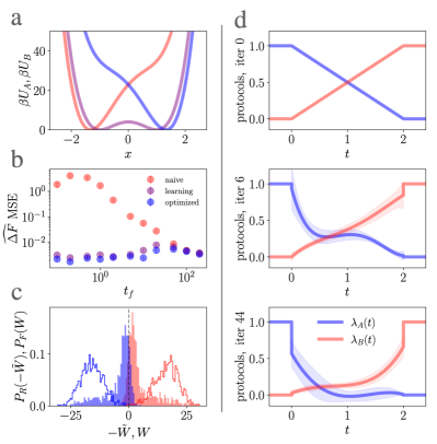
Figure 1: (a) The potentials $U_{A}({{x}})$ (red) and $U_{B}({{x}})$ (blue) are obtained by linearly biasing a double well (purple). (b) $\widehat{\Delta F}_{\mathrm{BAR}}$ mean squared error from 1000 bi-directional measurements drawn solely from the naive protocol (red), cumulatively from protocols that are adaptively optimized (“learning”) with our algorithm (purple), and solely from the last-iteration (“optimized”) protocols (blue) for various protocol times $t_{f}$. (c) Single-trial $\mathcal{P}_{F}(W)$ (red) and $\mathcal{P}_{R}(-\tilde{W})$ (blue) work distributions for 1000 measurements from the naive protocol, (unfilled) and adaptively optimized protocols (filled) for $t_{f}=2$, the ground truth shown as a grey dashed line. Measurements made with protocol optimization have significantly more overlap, leading to lower estimator error. (d) Forward protocols $\lambda_{A}(t)$ (blue) and $\lambda_{B}(t)$ (red) at various iterations of protocol optimization for $t_{f}=2$. Shaded region represents variability across $100$ independent trials. In the optimized last-iteration protocol, $\lambda_{A}(t)+\lambda_{B}(t)$ (giving the energy scale) is greatly reduced at intermediate times, while $\lambda_{B}(t)-\lambda_{A}(t)$ (giving the linear bias) is time-asymmetrically shifted. The reverse protocols (not shown here) are similar SM .

V.1 Linearly-Biased double well

The first system we consider is a one-dimensional quartic double-well with a linear bias (Fig. 1(a)). The potentials are $U_{A}(x)=E_{0}[(x^{2}-1)^{2}/4-x]$, $U_{B}(x)=E_{0}[(x^{2}-1)^{2}/4+x]$ (cf. Zhong and DeWeese (2022) for optimal protocols minimizing $\langle W_{\mathrm{trad}}\rangle_{F}$). We set $U_{C}(x)=0$ because $U_{B}(x)-U_{A}(x)$ is already linear in $x$. We use $\beta=1,E_{0}=16$, and a timestep $\Delta t=1\times 10^{-3}\tau$ where $\tau=1$ is the natural timescale (here the length scale, inverse temperature, and friction coefficient are all unity $\ell=\beta=\gamma=1$).

Fig. 1(b) displays the $\widehat{\Delta F}_{\mathrm{BAR}}$ estimator mean squared error for 1000 bi-directional work measurements collected solely from the naive protocol (red), the 1000 measurements collected cumulatively over on-the-fly protocol optimization (purple), and 1000 measurements collected solely from the last-iteration (blue). Each dot represents the empirical average over 100 independent trials. Note that the mean squared error is up to 1600 times lower under protocol optimization compared to under the naive protocol (obtained at $t_{f}=0.2$). For $t_{f}\gtrsim 10$ the algorithm does not converge within the 1000 measurements SM , leading to less improvement. Fig. 1(c) shows that bi-directional work measurements collected under the protocol optimization algorithm have significantly more overlap than measurements collected from the naive protocol, leading to reduced estimator error. Fig. 1(d) gives snapshots on how the optimal protocol is adaptively learned.

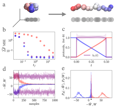
Figure 2: (a) A Rouse polymer is stretched from a collapsed state to an extended one. (b) $\widehat{\Delta F}_{\mathrm{BAR}}$ mean squared error verses protocol time, points colored as in Fig. 1. (c) For moderate protocol times ($t_{f}=0.5\,\tau_{\mathrm{R}}$ displayed here) the optimized protocol $(\lambda_{A}(t),\lambda_{B}(t),\lambda_{C}(t))$ learned in 44 iterations is the counterdiabatic protocol Eq. (31). (d) Single-trial bi-directional work samples from the naive protocol ($W$ and $-\tilde{W}$ purple) and adaptively-optimized protocols ($W$ red, $-\tilde{W}$ blue) for $t_{f}=0.5\,\tau_{\mathrm{R}}$. Vertical line demarcates start of protocol optimization. The ground truth $\Delta F$ is shown as a horizontal line. (e) Work distributions corresponding to the samples in (d). The ground truth is indicated by the triangular arrow. Cumulative measurements made under protocol optimization (filled) have dramatically greater overlap than measurements made under the naive protocols (unfilled), leading to lower estimator error.

V.2 Rouse polymer

Next we consider a $(N+1)$-bead Rouse polymer (Fig. 2(a)) with stiffness $k$ and intrinsic energy given by $U_{\mathrm{Rouse}}(x_{0},x_{1},...,x_{N})=\sum_{n=0}^{N-1}(k/2)(x_{n+1}-x_{n})^{2}$ from harmonic bonds between adjacent beads Doi et al. (1988); onl . We estimate $\Delta F$ between a collapsed state (fixing $x_{0}=x_{N}=0$) and an extended state (fixing $x_{0}=0$, $x_{N}=\lambda_{f}$), so our configuration space is ${{x}}\in\mathbb{R}^{N-1}$ with potential energies $U_{A}(x_{1},...,x_{N-1})=U_{\mathrm{Rouse}}(0,x_{1},...,x_{N-1},0)$ and $U_{B}(x_{1},...,x_{N-1})=U_{\mathrm{Rouse}}(0,x_{1},...,x_{N-1},\lambda_{f})$. Equilibrium averages $\langle x_{n}\rangle_{A}=0,\langle x_{n}\rangle_{B}=n\lambda_{f}/N$ give $U_{C}({{x}})=-(\lambda_{f}/Nt_{f})\sum^{N}_{n=1}nx_{n}$, and the ground truth is $\Delta F=F_{B}-F_{A}=k\lambda_{f}^{2}/(2N)$. It may be verified that for this problem the time-varying potential energies

$$U_{0}({{x}},t)=\bigg{(}1-\frac{t}{t_{f}}\bigg{)}U_{A}({{x}})+\bigg{(}\frac{t}{t_{f}}\bigg{)}U_{B}({{x}})$$

$$U_{1}({{x}},t)=U_{C}({{x}})$$ (31)

solve Eq. (9) and are thus counterdiabatic.

We use $\beta=k=1$, $N=20$, and timestep $\Delta t=2.5\,\times 10^{-5}\tau_{\mathrm{R}}$ where $\tau_{\mathrm{R}}=\beta N^{2}/\pi^{2}$ is the Rouse relaxation time Doi et al. (1988). Initial conditions for $\rho_{A}({{x}})$ and $\rho_{B}({{x}})$ were drawn from a normal-modes basis as described in SM Section II SM . Fig. 2(b) shows an improvement of up to $8300$ (for $t_{f}=0.5\,\tau_{\mathrm{R}}$) in $\widehat{\Delta F}_{\mathrm{BAR}}$ mean squared error between naive and optimized protocols. The counterdiabatic solution Eq. (31) corresponds to $\lambda_{A}(t)=(1-t/t_{f}),\lambda_{B}(t)=t/t_{f}$, and $\lambda_{C}(t)=1$, which what the algorithm learns for $t_{f}=\,\tau_{\mathrm{R}}$ as depicted in Fig. 2(c). (This was generally the case for $t_{f}\geq 0.5\,\tau_{\mathrm{R}}$. For $t_{f}<0.5\,\tau_{\mathrm{R}}$ the algorithm learns a sub-optimal local solution that still provides some improvement SM .) Fig. 2(d) shows single-trial traces of bi-directional work measurements for the naive protocol (purple) and adaptively-optimized protocols (red for $W$, blue for $-\tilde{W}$), for $t_{f}=0.5\tau_{\mathrm{R}}$. The protocol converges in $\sim 20$ iterations (requiring $\sim 500$ measurements), and then consistently gives work measurements closely centered at the ground truth free energy (gray horizontal line). Histograms of these traces (filled) are shown in Fig. 2(e), exhibiting a remarkable increase in the overlap compared with their naive counterparts (unfilled).

V.3 Worm-like chain with attractive linker

We now consider a $(N+1)$-bead worm-like chain model (WLC) in 2 dimensions with an added Lennard-Jones interaction between the first and last beads (similar to the 3rd example of Kuznets-Speck and Limmer (2023)). Fixing $(x_{0},y_{0})=(0,0)$, the configuration space is $\vec{\phi}\in\mathbb{R}^{N}$, where $\phi_{n}$ is the angle of the $n$th bond with respect to the $x$-axis, with $(x_{n}(\vec{\phi}),y_{n}(\vec{\phi}))=(\sum_{m=1}^{n}\cos\phi_{m},\sum_{m=1}^{n}\sin\phi_{m})$. The angular potential $U_{\phi}=k\sum^{N-1}_{n=1}[1-\cos(\phi_{n+1}-\phi_{n})]$ penalizes the bending of adjacent bonds, and $U_{\mathrm{LJ}}=4\epsilon_{\mathrm{LJ}}[(\sigma_{\mathrm{LJ}}/r_{N})^{12}-(\sigma_{\mathrm{LJ}}/r_{N})^{6}]$ specifies the interaction between first and last beads, where $r_{N}=\sqrt{x_{N}^{2}+y_{N}^{2}}$ is the end-to-end distance. We take $k=6,\beta=1,\epsilon_{\mathrm{LJ}}=8,\sigma_{\mathrm{LJ}}=4$, and $N=15$.

Fig. 3(a) displays the conditioned free energy $F(R/N):=-\beta^{-1}\ln\rho_{\mathrm{eq}}(r_{N}=R)$, where $\rho_{\mathrm{eq}}$ is the equilibrium probability of observing the end-to-end distance under $U=U_{\phi}+U_{\mathrm{LJ}}$ XY- (constructed from $10^{7}$ equilibrium samples of $U_{\phi}$, obtained with the Metropolis-adjusted Langevin Algorithm Roberts and Tweedie (1996), that were reweighted by $U_{\mathrm{LJ}}$). $F(R/N)$ exhibits a deep well for $R_{A}\approx 2^{1/6}\sigma_{\mathrm{LJ}}$ (trapped/bent state) and a shallow well at large $R_{B}\approx 0.9\,N$ (free/relaxed state), separated by a barrier; their difference in value $\Delta F\approx 4.18$ may be calculated by estimating the $\Delta F$ between $U_{A}(\vec{\phi})=U_{\phi}+U_{\mathrm{LJ}}+(k_{\mathrm{ext}}/2)(r_{N}-\lambda_{i})^{2}$ and $U_{B}(\vec{\phi})=U_{\phi}+U_{\mathrm{LJ}}+(k_{\mathrm{ext}}/2)(r_{N}-\lambda_{f})^{2}$ for $\lambda_{i}=2^{1/6}\sigma_{\mathrm{LJ}},\lambda_{f}=0.9\,N$, and $k_{\mathrm{ext}}\gg 1$.

We calculate the $\Delta F$ between $U_{A}$ and $U_{B}$ for $k_{\mathrm{ext}}=200$. We use timestep $\Delta t=1.41\times 10^{-4}\,\tau_{\mathrm{LJ}}$ where $\tau_{\mathrm{LJ}}=\sqrt{\epsilon_{\mathrm{LJ}}/\sigma^{2}}$ is the Lennard-Jones timescale. We use $U_{C}(\vec{\phi})=-\sum_{n}c_{n}r_{n}$, radially pulling on each individual bead, constructed with $c_{n}=(\langle r_{n}\rangle_{B}-\langle r_{n}\rangle_{A})/t_{f}$ from equilibrium samples of $\rho_{A}$ and $\rho_{B}$. Fig. 3(b) displays single-trial work histograms for $t_{f}=0.71\,\tau_{\mathrm{LJ}}$, showing work measurements much closer to the ground truth with protocol optimization, compared to the naive protocol. Fig. 3(c) shows the updating $\widehat{\Delta F}_{\mathrm{BAR}}$ estimator over 100 independent trials converges substantially faster to the ground truth. With 1000 bi-directional samples under the naive protocol the mean squared error is $1.62\ (k_{\mathrm{B}}T)$; under protocol optimization, only 160 samples (i.e., just after two iterations of protocol optimization) are required to have a smaller mean squared error. Over various $t_{f}$, the mean squared error is up to 120 times lower under protocol optimization compared to under the naive protocol SM .

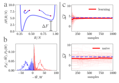
Figure 3: Worm-like chain with an attractive linker. (a) Ground truth free energy surface relative to its value at $R_{A}=2^{1/6}\sigma_{\mathrm{LJ}}$; the left well corresponds to the ends of the chain bound to one another and the right well corresponds to a nearly straight configuration, with a free energy difference $\Delta F\approx 4.18$. (b) Work distributions before (unfilled) and during (filled) optimization for $t_{f}=0.71$, the ground truth shown as a grey dashed line. (c) The $\widehat{\Delta F}_{\mathrm{BAR}}$ estimator updated over the $1000$ samples converges to the ground truth value (dashed blue line) much more quickly under protocol optimization than under the naive protocol. At $1000$ samples the protocol optimization free energy estimate was $\widehat{\Delta F}=3.94\pm 0.11$, while for the naive protocol was $\widehat{\Delta F}=3.52\pm 1.48$ (c.f. ground truth value of $\Delta F=4.18$). It took $200$ total samples for the mean squared error to drop below $1.00\,(k_{\mathrm{B}}T)$ under protocol optimization.

VI Discussion

In this paper, we derived the time-asymmetric microscopic fluctuation theorem for the unconventional work introduced by Vaikuntanathan and Jarzynski (2008). We then demonstrated its practical utility for free energy estimation by presenting an adaptive time-asymmetric protocol optimization algorithm, whose effectiveness we illustrated with three toy models of varying complexity. Time-asymmetric protocols have been considered before Li et al. (2017); Li and Tu (2019); Blaber and Sivak (2020), but to our knowledge we are the first to use $\widehat{\Delta F}_{\mathrm{BAR}}$ on bi-directional work measurements from adaptive time-asymmetric protocols. A clear next step is to test our algorithm on more physically realistic systems. This work should be straightforward to implement with JAX-MD Schoenholz and Cubuk (2020). In principle our algorithm should work with underdamped dynamics SM ; Li and Tu (2019), and it should also be possible to adaptively optimize the protocol time $t_{f}$ and sampling ratio $n_{F}/n_{R}$. Another future direction to pursue is to differentially weight early versus later samples in the estimator to account for differences in the variance of work measurements, as the algorithm more closely approximates a counterdiabatic protocol.

The fast convergence in our method comes from exploiting of the quadratic structure of the Onsager-Machlup path action to construct $\hat{J}(\theta)$, which allows all samples to be used in each optimization step. Typically the most computationally expensive step in a molecular dynamics simulation is calculating potential energy gradients $\nabla U$ to evolve $X(t)$, which does not need to be repeated to evolve $(\mathsf{a}_{\mu\nu},\mathsf{b}_{\mu},...)$. A valid critique of our algorithm is that the number of auxiliary variables included with each trajectory scales quadratically with the number of basis functions, becoming prohibitively large when considering, for example, a separate control force on each particle of a many particle system. However, we have shown that a small number of basis functions to represent Eq. (28) already produces a substantial improvement in efficiency for our three examples. That said, it is straightforward to add additional basis functions (cf. Eq. (2) of Naden et al. (2014)), which may be useful for more complex and realistic systems. It would be interesting to apply recent methods Singh and Limmer (2023) to learn the optimal set of additional basis functions, that apply force along specific coordinates: bonds, angles, native contacts and other collective variables to further improve performance for larger scale systems.

As mentioned at the end of the Introduction, our results were independently derived in Vargas and Nüsken (2023) within a machine learning context. It is noteworthy that stochastic thermodynamics has shown to be a useful theoretical framework not only for non-equilibrium statistical physics, but also for machine learning in flow-based diffusion models Sohl-Dickstein et al. (2015); Song et al. (2020); Doucet et al. (2022); Albergo et al. (2023). In particular, we recognize significant ties between our work, and that of “Stochastic Normalizing Flows” Wu et al. (2020), wherein authors also consider constructing counterdiabatic protocols under the name “deterministic invertible functions”. It can be shown that counterdiabatic protocols are perfect stochastic normalizing flows, and they report (after sufficient neural-network training) excellent numerical results for sampling and free energy estimation. The primary difference is that in their work they fix $U_{0}=(1-t/t_{f})U_{A}+(t/t_{f})U_{B}$ and use a neural-network ansatz, whereas here we use an adaptive importance sampling algorithm with a linear spatio-temporal basis ansatz for both $U_{0}$ and $U_{1}$. Likewise, we note Bernton et al. (2019) explores time-asymmetric Markovian processes for sampling, building off of entropy-regularized optimal transport wherein solutions of the continuous-time Schrödinger bridge problem involve asymmetrically-controlled diffusion processes Chen et al. (2021) (see also De Bortoli et al. (2021); Berner et al. (2022)). This is intriguing, as solving for optimal time-symmetric protocols has been shown to be equivalent to solving the continuous-time formulation Benamou and Brenier (2000) of standard optimal transport Aurell et al. (2011); Chen et al. (2019); Nakazato and Ito (2021); Zhong and DeWeese (2022); Chennakesavalu and Rotskoff (2023). In light of all this, we suspect deep theoretical connections between stochastic thermodynamics and machine learning may be further uncovered through the time-asymmetric fluctuation theorem.

Documented code for this project may be found at https://github.com/adrizhong/dF-protocol-optimization.

Appendix A Microscopic fluctuation theorem

A.1 The Onsager-Machlup Action

For overdamped Langevin dynamics for $X(t)\in\mathbb{R}^{d}$,

$$\dot{X}=-\nabla U(X(t),t)+\sqrt{2\beta^{-1}}\,\eta(t)\quad\mathrm{with}\quad X(0)\sim\rho(\cdot),$$ (32)

where $\eta(t)$ is an instantiation of standard Gaussian white noise with statistics $\langle\eta_{i}(t)\rangle=0$ and $\langle\eta_{i}(t)\eta_{j}(t^{\prime})\rangle=\delta_{ij}\delta(t-t^{\prime})$, and $\rho(\cdot)$ is its initial distribution, the formal expression for the probability of a path’s realization is (up to a multiplicative factor)

$$\mathcal{P}[X(t)]=\rho(X(0))e^{-\beta S[X(t)]}.$$ (33)

Here $S[X(t)]$ is the Onsager-Machlup Path Action functional

$$S[X(t)]=(\mathrm{I})\int_{0}^{t_{f}}\frac{|\dot{X}(t)+\nabla U(X(t),t)|^{2}}{4}\,\mathrm{d}t$$ (34)

which comes from the path discretization into $N$ timesteps with timestep $\Delta t=t_{f}/N$: $X(t)\rightarrow[X_{0},X_{1},...\,,X_{N}]$, with $X_{n}\approx X(t_{n})$, $N=t_{f}/\Delta t$, and $t_{n}=n\Delta t$, generated from Euler-Maruyama dynamics

$$X_{0}\sim\rho(\cdot)$$ (35)

$$X_{n+1}=X_{n}-\nabla U(X_{n},t_{n})\,\Delta t+\sqrt{2\beta^{-1}}\,\Delta B_{n},$$ (36)

where $\Delta B_{n}\sim\mathcal{N}(0,\Delta t\,I_{d})$ is a $d$-dimensional Gaussian random variable (i.e., Brownian increment) Adib (2008).

The probability of the realization of a particular path is then

$$\mathcal{P}(X_{0},X_{1},...\,,X_{N}) =\mathcal{P}(X_{0})\mathcal{P}(X_{1}|X_{0})\mathcal{P}(X_{2}|X_{1})...\mathcal{P}(X_{N}|X_{N-1})$$

$$=\rho(X_{0})\prod_{n=0}^{N-1}(4\pi\beta^{-1}\Delta t)^{-d/2}\exp\bigg{(}-\frac{|X_{n+1}-X_{n}+\nabla U(X_{n},t_{n})\Delta t|^{2}}{4\beta^{-1}\Delta t}\bigg{)}$$

$$\propto\rho(X_{0})\exp\bigg{(}-\beta\sum_{n=0}^{N-1}\frac{|(\frac{X_{n+1}-X_{n}}{\Delta t})+\nabla U(X_{n},t_{n})|^{2}}{4}\Delta t\bigg{)},$$ (37)

where the normalization factor $(4\pi\beta^{-1}\Delta t)^{-Nd/2}$ is hidden in the last line.

Taking $N\rightarrow\infty$ with $\Delta t=t_{f}/N\rightarrow 0$, the sum within the exponential becomes

$$\sum_{n=0}^{N-1}\frac{|(\frac{X_{n+1}-X_{n}}{\Delta t})+\nabla U(X_{n},t_{n})|^{2}}{4}\Delta t$$

$$\quad\longrightarrow\quad(\mathrm{I})\int_{0}^{t_{f}}\frac{|\dot{X}(t)+\nabla U(X(t),t)|^{2}}{4}\mathrm{d}t=S[X(t)],$$ (38)

which yields the formal expression Eq. (33).

A.2 Stochastic Integrals and Itô’s formula

Here we briefly review the rules of stochastic calculus. For a stochastic path (i.e., a “Brownian motion”) $X(t)|_{t\in[0,t_{f}]}$ from Eq. (32) and some vector-valued function $b({{x}},t)$, the three following choices for the time-discretization of the integral $\int_{0}^{t_{f}}b(X(t),t)\cdot\dot{X}(t)\,\mathrm{d}t$ :

$$\sum_{n=0}^{N-1}b(X_{n},t_{n})\cdot\Delta X_{n},$$

$$\sum_{n=0}^{N-1}b(X_{n+\frac{1}{2}},t_{n+\frac{1}{2}})\cdot\Delta X_{n},$$

and

$$\sum_{n=0}^{N-1}b(X_{n+1},t_{n+1})\cdot\Delta X_{n}$$

(here $\Delta X_{n}=(X_{n+1}-X_{n})$, $X_{n+\frac{1}{2}}=(X_{n}+X_{n+1})/2$, and $t_{n+\frac{1}{2}}=(t_{n}+t_{n+1})/2$) do not necessarily converge to the same value under the $N\rightarrow\infty$, $\Delta t=t_{f}/N\rightarrow 0$ limit. This is in contrast to the case where $X(t)|_{t\in[0,t_{f}]}$ is continuously differentiable, e.g., the solution of a well-behaved deterministic differential equation, in which case the above three time-discretizations do converge to the same integral value under the limit Pugh and Pugh (2002).

Therefore, for trajectories $X(t)|_{t\in[0,t_{f}]}$ obtained through the stochastic differential equation Eq. (32), we must define each of these as distinct integrals

$$(\mathrm{I})\int_{0}^{t_{f}}b(X(t),t)\cdot\dot{X}\,\mathrm{d}t:=\lim_{N\rightarrow\infty}\sum_{n=0}^{N-1}b(X_{n},t_{n})\cdot\Delta X_{n},$$

$$(\mathrm{S})\int_{0}^{t_{f}}b(X(t),t)\cdot\dot{X}\,\mathrm{d}t:=\lim_{N\rightarrow\infty}\sum_{n=0}^{N-1}b(X_{n+\frac{1}{2}},t_{n+\frac{1}{2}})\cdot\Delta X_{n},$$

and

$$(\mathrm{BI})\int_{0}^{t_{f}}b(X(t),t)\cdot\dot{X}\,\mathrm{d}t:=\lim_{N\rightarrow\infty}\sum_{n=0}^{N-1}b(X_{n+1},t_{n+1})\cdot\Delta X_{n},$$

which are the Itô, Stratonovich, and Backwards Itô integrals, respectively. They are related to one another by Itô’s lemma Oksendal (2013)

$$(\mathrm{I})\int_{0}^{t_{f}}b(X(t),t)\cdot\dot{X}+\beta\,\nabla\cdot b(X(t),t)\,\mathrm{d}t$$

$$\quad=(\mathrm{S})\int_{0}^{t_{f}}b(X(t),t)\cdot\dot{X}\,\mathrm{d}t$$

$$\quad\quad=(\mathrm{BI})\int_{0}^{t_{f}}b(X(t),t)\cdot\dot{X}-\beta\,\nabla\cdot b(X(t),t)\,\mathrm{d}t.$$ (39)

The Stratonovich integration convention (i.e., with the time-symmetric midpoint-rule discretization) is particularly convenient because ordinary calculus rules (e.g., the chain rule, product rule, etc.) apply.

Note that the three separate time-discretizations of integrals of the form $\int_{0}^{t_{f}}f(X(t),t)\,\mathrm{d}t$ :

$$\sum_{n=0}^{N-1}f(X_{n},t_{n})\,\Delta t,$$

$$\sum_{n=0}^{N-1}f(X_{n+\frac{1}{2}},t_{n+\frac{1}{2}})\,\Delta t,$$

and

$$\quad\sum_{n=0}^{N-1}f(X_{n+1},t_{n+1})\,\Delta t$$

do converge to the same value under the $N\rightarrow\infty$ with $\Delta t=t_{f}/N\rightarrow 0$ limit, thus $(\mathrm{I})\int_{0}^{t_{f}}f(X(t),t)\,\mathrm{d}t=(\mathrm{S})\int_{0}^{t_{f}}f(X(t),t)\,\mathrm{d}t=(\mathrm{BI})\int_{0}^{t_{f}}f(X(t),t)\,\mathrm{d}t$.

A.3 Microscopic fluctuation theorem derivation

Here, we use the stochastic calculus reviewed above to derive Eq. (13), i.e., the equivalence of its first and second lines. We start by manipulating the expression within the exponent

$$U_{A}(X(0))+S[X(t)]+W[X(t)]=U_{B}(X(t_{f}))+(\mathrm{I})\int_{0}^{t_{f}}\bigg{\{}\frac{|\dot{X}+\nabla(U_{0}+U_{1})|^{2}}{4}-(\dot{X}+\nabla U_{1})\cdot\nabla U_{0}+\beta^{-1}\nabla^{2}(U_{1}-U_{0})\bigg{\}}\,\mathrm{d}t$$

$$=U_{B}(X(t_{f}))+\frac{1}{4}(\mathrm{I})\int_{0}^{t_{f}}|\dot{X}|^{2}\,\mathrm{d}t+\frac{1}{4}(\mathrm{I})\int_{0}^{t_{f}}|\nabla(U_{1}-U_{0})|^{2}\,\mathrm{d}t+\frac{1}{2}(\mathrm{I})\int_{0}^{t_{f}}\dot{X}\cdot\nabla(U_{1}-U_{0})+2\beta\nabla^{2}(U_{1}-U_{0})\,\mathrm{d}t$$

$$=U_{B}(X(t_{f}))+\frac{1}{4}(\mathrm{BI})\int_{0}^{t_{f}}|\dot{X}|^{2}\,\mathrm{d}t+\frac{1}{4}(\mathrm{BI})\int_{0}^{t_{f}}|\nabla(U_{1}-U_{0})|^{2}\,\mathrm{d}t+\frac{1}{2}(\mathrm{BI})\int_{0}^{t_{f}}\dot{X}\cdot\nabla(U_{1}-U_{0})\,\mathrm{d}t$$

$$=U_{B}(X(t_{f}))+(\mathrm{BI})\int_{0}^{t_{f}}\frac{|\dot{X}+\nabla(U_{1}-U_{0})|^{2}}{4}\,\mathrm{d}t$$

$$=U_{B}(\tilde{X}(0))+(\mathrm{I})\int_{0}^{t_{f}}\frac{|-\dot{\tilde{X}}+\nabla(\tilde{U}_{1}-\tilde{U}_{0})|^{2}}{4}\,\mathrm{d}t$$

$$=U_{B}(\tilde{X}(0))+\tilde{S}[\tilde{X}(t)],\quad\mathrm{where}\quad\tilde{S}[\tilde{X}(t)]=(\mathrm{I})\int_{0}^{t_{f}}\frac{|\dot{\tilde{X}}+\nabla(\tilde{U}_{0}-\tilde{U}_{1})|^{2}}{4}\,\mathrm{d}t.$$ (40)

The first equality comes from using Ito’s lemma $U_{0}(X(t_{f}),t_{f})-U_{0}(X(0),0)=(\mathrm{I})\int_{0}^{t_{f}}\partial_{t}U_{0}+\dot{X}\cdot\nabla U_{0}\,+\beta^{-1}\nabla^{2}U_{0}\,\mathrm{d}t$. The second equality follows from standard algebraic manipulation. The third equality comes from converting the Forward Itô integrals $(\mathrm{I})$ to Backward Itô integrals $(\mathrm{BI})$ using Itô’s formula Eq. (39). The fourth equality results from standard algebraic manipulation. The fifth equality comes from the time-reversal transformation $t\rightarrow t_{f}-t$, with the Backward Itô integral becoming a forward Itô integral under time-reversal.

Finally, we plug in the above to the first line of Eq. (13) to obtain

$$\tilde{\mathcal{P}}[\tilde{X}(t)] =e^{-\beta\{U_{A}(X(0))-F_{A}+S[X(t)]+W[X(t)]-\Delta F\}}$$

$$=e^{-\beta\{U_{B}(\tilde{X}(0))-F_{B}+\tilde{S}[\tilde{X}(t)]\}}$$

$$=\rho_{B}(\tilde{X}(0))e^{-\beta\tilde{S}[\tilde{X}(t)]},$$ (41)

thus completing our derivation.

Appendix B Deriving the fluctuation theorem from the microscopic fluctuation theorem

In this section we derive the Crooks Fluctuation Theorem

$$\frac{\mathcal{P}_{F}(+W)}{\mathcal{P}_{R}(-W)}=e^{+\beta(W-\Delta F)}$$ (42)

from the microscopic fluctuation theorem

$$\mathcal{P}[X(t)]e^{-\beta W[X(t)]}=\tilde{\mathcal{P}}[\tilde{X}(t)]e^{-\beta\Delta F}.$$ (43)

We begin by recalling that $\mathcal{P}_{F}(\cdot)$, giving the probability of observing a particular work value in the forward ensemble, is defined as

$$\mathcal{P}_{F}(w) =\langle\delta(W-w)\rangle_{F}$$

$$=\int DX(t)\mathcal{P}[X(t)]\delta(W[X(t)]-w),$$ (44)

where we write $w$ to distinguish the argument of $\mathcal{P}_{F}(\cdot)$ from the path-functional work $W=W[X(t)]$. Here $DX(t)$ denotes an integral over all paths $X(t)|_{t\in[0,t_{f}]}$, $\mathcal{P}[X(t)]$ is the probability of its realization, and $\delta(\cdot)$ is the Dirac-delta function. Plugging in Eq. (43) to the above expression, we get

$$\mathcal{P}_{F}(w) =\int DX(t)\tilde{\mathcal{P}}[\tilde{X}(t)]e^{+\beta\{W[X(t)]-\Delta F\}}\delta(W[X(t)]-w)$$

$$=e^{+\beta(w-\Delta F)}\int DX(t)\tilde{\mathcal{P}}[\tilde{X}(t)]\delta(W[X(t)]-w)$$

$$=e^{+\beta(w-\Delta F)}\int D\tilde{X}(t)\tilde{\mathcal{P}}[\tilde{X}(t)]\delta(-\tilde{W}[\tilde{X}(t)]-w)$$

$$=e^{+\beta(w-\Delta F)}\mathcal{P}_{R}(-w),$$ (45)

where in the second line we pull out the exponential using the Dirac delta function, in the third line we consider the coordinate change $X(t)\rightarrow\tilde{X}(t)$ (using also $\tilde{W}[\tilde{X}(t)]=-W[X(t)]$, see Eq. (16) and the text that follows it in the main article), and in the fourth line we have recognized that the path integral expression is equivalent to the probability of observing the work value $-w$ in the reverse path ensemble.

References

• Cournia et al. (2017) Z. Cournia, B. Allen,  and W. Sherman, Journal of chemical information and modeling 57, 2911 (2017).
• Tawa et al. (1998) G. Tawa, I. Topol, S. Burt, R. Caldwell,  and A. Rashin, The Journal of Chemical Physics 109, 4852 (1998).
• Kelly et al. (2006) C. P. Kelly, C. J. Cramer,  and D. G. Truhlar, The Journal of Physical Chemistry B 110, 16066 (2006).
• Chipot and Pohorille (2007) C. Chipot and A. Pohorille, Free energy calculations, Vol. 86 (Springer, 2007).
• Shirts et al. (2010) M. R. Shirts, D. L. Mobley,  and S. P. Brown, Drug Design 1, 61 (2010).
• Cournia et al. (2021) Z. Cournia, C. Chipot, B. Roux, D. M. York,  and W. Sherman, in Free Energy Methods in Drug Discovery: Current State and Future Directions (ACS Publications, 2021) pp. 1–38.
• (7) In this paper, to avoid confusion we use lower case $x$ to denote configurations, and upper case $X(t)$ to denote (stochastic) trajectories.
• Shirts and Pande (2005) M. R. Shirts and V. S. Pande, The Journal of chemical physics 122, 144107 (2005).
• Shirts et al. (2003) M. R. Shirts, E. Bair, G. Hooker,  and V. S. Pande, Physical review letters 91, 140601 (2003).
• Bennett (1976) C. H. Bennett, Journal of Computational Physics 22, 245 (1976).
• Crooks (1998) G. E. Crooks, Journal of Statistical Physics 90, 1481 (1998).
• Crooks (1999) G. E. Crooks, Physical Review E 60, 2721 (1999).
• Vaikuntanathan and Jarzynski (2008) S. Vaikuntanathan and C. Jarzynski, Physical Review Letters 100, 190601 (2008).
• Zhong et al. (2023) A. Zhong, B. Kuznets-Speck,  and M. R. DeWeese, arXiv preprint arXiv:2304.12287  (2023).
• Vargas and Nüsken (2023) F. Vargas and N. Nüsken, arXiv preprint arXiv:2307.01050  (2023).
• (16) Typically there is a factor of the friction coefficient $\gamma$ multiplying the left side of (6). For notational simplicity we have set it to one, which given that it is equal for all dimensions may always be done through a time-rescaling.
• (17) Supplementary material may be found at [url].
• del Campo (2013) A. del Campo, Physical review letters 111, 100502 (2013).
• Guéry-Odelin et al. (2019) D. Guéry-Odelin, A. Ruschhaupt, A. Kiely, E. Torrontegui, S. Martínez-Garaot,  and J. G. Muga, Reviews of Modern Physics 91, 045001 (2019).
• Ilker et al. (2022) E. Ilker, Ö. Güngör, B. Kuznets-Speck, J. Chiel, S. Deffner,  and M. Hinczewski, Physical Review X 12, 021048 (2022).
• Iram et al. (2021) S. Iram, E. Dolson, J. Chiel, J. Pelesko, N. Krishnan, Ö. Güngör, B. Kuznets-Speck, S. Deffner, E. Ilker, J. G. Scott, et al., Nature Physics 17, 135 (2021).
• Frim et al. (2021) A. G. Frim, A. Zhong, S.-F. Chen, D. Mandal,  and M. R. DeWeese, Physical Review E 103, L030102 (2021).
• Adib (2008) A. B. Adib, The Journal of Physical Chemistry B 112, 5910 (2008).
• Tang and Abbeel (2010) J. Tang and P. Abbeel, Advances in Neural Information Processing Systems 23 (2010).
• (25) The astute reader might point out that under the rules of stochastic calculus, how they are written out $\mathsf{a}=\mathsf{\tilde{a}}$ for all ${{x}}(t)$. However, they are different under a finite time-discretization, and thus must both be kept track.
• Williams (1992) R. J. Williams, Reinforcement learning , 5 (1992).
• Peters and Schaal (2008) J. Peters and S. Schaal, Neural networks 21, 682 (2008).
• Warren and Allen (2012) P. B. Warren and R. J. Allen, Physical review letters 109, 250601 (2012).
• Das and Limmer (2019) A. Das and D. T. Limmer, The Journal of chemical physics 151, 244123 (2019).
• Das et al. (2022) A. Das, B. Kuznets-Speck,  and D. T. Limmer, Physical Review Letters 128, 028005 (2022).
• Owen (2013) A. B. Owen, Monte Carlo theory, methods and examples (2013).
• Kraft (1988) D. Kraft, Forschungsbericht- Deutsche Forschungs- und Versuchsanstalt fur Luft- und Raumfahrt  (1988).
• Virtanen et al. (2020) P. Virtanen, R. Gommers, T. E. Oliphant, M. Haberland, T. Reddy, D. Cournapeau, E. Burovski, P. Peterson, W. Weckesser, J. Bright, S. J. van der Walt, M. Brett, J. Wilson, K. J. Millman, N. Mayorov, A. R. J. Nelson, E. Jones, R. Kern, E. Larson, C. J. Carey, İ. Polat, Y. Feng, E. W. Moore, J. VanderPlas, D. Laxalde, J. Perktold, R. Cimrman, I. Henriksen, E. A. Quintero, C. R. Harris, A. M. Archibald, A. H. Ribeiro, F. Pedregosa, P. van Mulbregt,  and SciPy 1.0 Contributors, Nature Methods 17, 261 (2020).
• (34) The first two terms are a generalization of the protocol form $U_{\lambda}({{x}})=(1-\lambda)\,U_{A}({{x}})+\lambda\,U_{B}({{x}})$ commonly considered in stochastic thermodynamics. Typically, linear combinations of just $U_{A}({{x}})$ and $U_{B}({{x}})$ are not effective in transporting $\rho_{A}({{x}})\rightarrow\rho_{B}({{x}})$, motivating our inclusion of the linear potential $U_{C}({{x}})$.
• Zhong and DeWeese (2022) A. Zhong and M. R. DeWeese, Physical Review E 106, 044135 (2022).
• Doi et al. (1988) M. Doi, S. F. Edwards,  and S. F. Edwards, The theory of polymer dynamics, Vol. 73 (oxford university press, 1988).
• (37) Because of the harmonic nature of the interbead potential, the dynamics of the Rouse polymer separates in its 3 spatial dimensions; without loss of generality, we can consider just a single spatial dimension.
• Kuznets-Speck and Limmer (2023) B. Kuznets-Speck and D. T. Limmer, Biophysical Journal 122, 1659 (2023).
• (39) From the change of coordinates $R=\sqrt{x_{N}^{2}+y_{N}^{2}},\vartheta=\tan^{-1}(y_{N}/x_{N})$ and the radial symmetry of $U_{\phi}$ and $U_{\mathrm{LJ}}$, one has $\rho_{\mathrm{eq}}(R)\propto(2\pi R)^{-1}\rho_{\mathrm{eq}}(x_{N}=R,y_{N}=0)$.
• Roberts and Tweedie (1996) G. O. Roberts and R. L. Tweedie, Bernoulli , 341 (1996).
• Li et al. (2017) G. Li, H. Quan,  and Z. Tu, Physical Review E 96, 012144 (2017).
• Li and Tu (2019) G. Li and Z. Tu, Physical Review E 100, 012127 (2019).
• Blaber and Sivak (2020) S. Blaber and D. A. Sivak, The Journal of Chemical Physics 153, 244119 (2020).
• Schoenholz and Cubuk (2020) S. Schoenholz and E. D. Cubuk, Advances in Neural Information Processing Systems 33, 11428 (2020).
• Naden et al. (2014) L. N. Naden, T. T. Pham,  and M. R. Shirts, Journal of Chemical Theory and Computation 10, 1128 (2014).
• Singh and Limmer (2023) A. N. Singh and D. T. Limmer, arXiv preprint arXiv:2302.14857  (2023).
• Sohl-Dickstein et al. (2015) J. Sohl-Dickstein, E. Weiss, N. Maheswaranathan,  and S. Ganguli, in International conference on machine learning (PMLR, 2015) pp. 2256–2265.
• Song et al. (2020) Y. Song, J. Sohl-Dickstein, D. P. Kingma, A. Kumar, S. Ermon,  and B. Poole, arXiv preprint arXiv:2011.13456  (2020).
• Doucet et al. (2022) A. Doucet, W. Grathwohl, A. G. Matthews,  and H. Strathmann, Advances in Neural Information Processing Systems 35, 21482 (2022).
• Albergo et al. (2023) M. S. Albergo, N. M. Boffi,  and E. Vanden-Eijnden, arXiv preprint arXiv:2303.08797  (2023).
• Wu et al. (2020) H. Wu, J. Köhler,  and F. Noé, Advances in Neural Information Processing Systems 33, 5933 (2020).
• Bernton et al. (2019) E. Bernton, J. Heng, A. Doucet,  and P. E. Jacob, arXiv preprint arXiv:1912.13170  (2019).
• Chen et al. (2021) Y. Chen, T. T. Georgiou,  and M. Pavon, Siam Review 63, 249 (2021).
• De Bortoli et al. (2021) V. De Bortoli, J. Thornton, J. Heng,  and A. Doucet, Advances in Neural Information Processing Systems 34, 17695 (2021).
• Berner et al. (2022) J. Berner, L. Richter,  and K. Ullrich, arXiv preprint arXiv:2211.01364  (2022).
• Benamou and Brenier (2000) J.-D. Benamou and Y. Brenier, Numerische Mathematik 84, 375 (2000).
• Aurell et al. (2011) E. Aurell, C. Mejía-Monasterio,  and P. Muratore-Ginanneschi, Physical review letters 106, 250601 (2011).
• Chen et al. (2019) Y. Chen, T. T. Georgiou,  and A. Tannenbaum, IEEE transactions on automatic control 65, 2979 (2019).
• Nakazato and Ito (2021) M. Nakazato and S. Ito, Physical Review Research 3, 043093 (2021).
• Chennakesavalu and Rotskoff (2023) S. Chennakesavalu and G. M. Rotskoff, Physical Review Letters 130, 107101 (2023).
• Pugh and Pugh (2002) C. C. Pugh and C. Pugh, Real mathematical analysis, Vol. 2011 (Springer, 2002).
• Oksendal (2013) B. Oksendal, Stochastic differential equations: an introduction with applications (Springer Science & Business Media, 2013).