On local stability threshold of del Pezzo surfaces

Abstract

We complete the classification of local stability thresholds for smooth del Pezzo surfaces of degree 2. In particular, we show that this number is irrational if and only if the tangent plane at the point intersecting the surface is the union of a line and a smooth cubic curve meeting transversally at the point.

1 Introduction

K-stability is an algebraic condition that detects the existence of Kähler-Einstein metrics on Fano varieties [Tia97, Don02, Tia15, LXZ22, CDS15]. It also provides the right framework to construct compact moduli for Fano varieties [ABHLX20, BHLLX21, BLX22, BX19, Jia18, LWX21, LXZ22, Xu20, XZ20].

An explicit verification of K-stability has become possible thanks to valuative criteria, see [FO18, BJ20, LXZ22]. It can be defined by numerical invariants, for instance the so called stability threshold $\delta$. In this paper, we will focus on the study $\delta$, mostry in local situation.
It was originally conjectured that $\delta(X)$ is rational for K-polystable Fano varieties, and was proven by Liu, Xu, and Zhuang in [LXZ22] for $\delta(X)<(n+1)/n$ where $n$ is the dimension of $X$. However, the local stability threshold, $\delta_{p}(X)$, is more mysterious. It is not always rational and it is not known how their rationality behaves. Note that $\delta(X)$ is the infimum of $\delta_{p}(X)$ for all $p\in X$. The only known example where the local delta invariant is irrational is in cubic surfaces (see [AZ22, Lemma A.6]). It is already known that $\delta_{p}(X)$ is rational for every point $p$ when $X$ is a del Pezzo surface of degree equal to or greater than 4 (see [ACC⁺23, §2]). In fact, even local delta invariants of weak del Pezzo surfaces of degree equal to or greater than 4 are rational by recent studies of Akaike and Denisova [Aka23, Den]. It is worth mentioning that no such study has been carried out in higher dimensions. It is expected that irrational $\delta_{p}$ exists only for certain points $p$ in del Pezzo surfaces of degrees 1, 2, and 3. In this paper, we settle this in degree 2 with the following theorem.

Theorem 1.1.

Let $X\subset\mathbb{P}(1,1,1,2)$ be a smooth del Pezzo surface of degree 2 and let $p=(x,y,z,w)\in X$ be a closed point with $w\neq 0$. Let $Q=T_{p}(X)\cap X$ be the tangent hyperplane section. Assume that $Q=L\cup C$ where $L$ is a line meeting the cubic $C$ transversally at $p$. Then $\delta_{p}(X)=\frac{6}{71}(11+8\sqrt{3})$ and it is computed by the weighted blow up at $p$ with $\operatorname{wt}(u)=2$ and $\operatorname{wt}(v)=\sqrt{3}$ (where $u$ and $v$ are the local coordinates such that $L=\{u=0\}$ and $C=\{v-u^{2}-u^{3}=0\}$.

It is straightforward to find examples of del Pezzo surfaces of degree 2 that satisfy the conditions of the theorem just by looking at the general equation given at the beginning of §3.

Sketch of the proof.

In order to prove that the local stability threshold at $p_{0}$ is irrational, we follow these steps: First, we take $E_{a,b}$ to be the exceptional divisor of a certain weighted blowup at $p_{0}$ with weights $(a,b)$. The choice of $(a,b)$ becomes clear in §5. Using that exceptional divisor we compute an upper bound for $\delta_{p_{0}}(X)$. The difficulty here is to compute the expected vanishing order of the anticanonical divisor of $X$ with respect to the exceptional divisor $E_{a,b}$, which requires a Zariski Decomposition and a careful choice of negative curves in the weighted blowup of $X$. This is the main bulk of the work in section §4.2.
Then, we use techniques from [AZ22] to find lower bounds for $\delta_{p_{0}}(X)$, which requires a delicate choice of a minimazer sequence of prime divisors $E_{a_{m},b_{m}}$ over $X$. The choice of $a$, $b$ is made so that this bound is exactly the upper bound found earlier by considering $E_{a,b}$. In other words, we compute $\delta_{p_{0}}(X)$.

Acknowledgements:

I thank Hamid Abban for suggesting the problem to me and his constant guidance. Moreover, I want to thank Tiago Duarte Guerreiro, Luca Giovanzana, James Jones, Antonio Trusiani, Nivedita Viswanathan and Ziquan Zhuang for numerous discussions and the interest shown.

2 Preliminary results and definitions

2.1 Singularities

In this paper we work over $\mathbb{C}$ and all varieties are assumed to be normal and projective.

Definition 2.1.

A logarithmic pair (also called a log pair) is a pair $(X,D)$ consisting of a normal variety $X$ and a boundary $\mathbb{Q}$-divisor $D$. A boundary divisor $D=\sum d_{k}D_{k}$ is a divisor with rational coefficients between $0$ and $1$, i.e. $0\leq d_{k}\leq 1$, where the $D_{k}$ are prime divisors. We call $K_{X}+D$ the log canonical divisor of the pair $(X,D)$.

Definition 2.2.

Let $(X,D)$ be a log pair. Assume that $K_{X}+D$ is $\mathbb{Q}$-Cartier. Let $f:V\to X$ be a birational morphism from a nonsingular variety $V$. Write the ramification formula:

$$K_{V}=f^{*}(K_{X}+D)-f_{*}^{-1}(D)+\sum a(E;X,D)E,$$

where the sum runs over $f$-exceptional divisors $E$. Recall that $a(E;X,D)$ is a rational number independent of the morphism $f$ and depends only on the discrete valuation which corresponds to $E$. This is called the discrepancy of the pair $(X,D)$ at $E$. The log discrepancy of the pair $(X,D)$ at $E$ is defined to be

$$A_{X,D}(E)=a(E;X,D)+1.$$

There is a more general definition of log discrepancy in [LXZ22, Def. 2.5].

Since we are working with Fano surfaces, it is essential to recall the characterization for ampleness and other properties of divisors which you can find in different references such as [Mat02, Laz04].

Definition 2.3.

Let $r>0$ and $a_{1},...,a_{n}$ be integers and let $x_{1},...,x_{n}$ be coordinates on $\mathbb{A}^{n}$. Suppose that $\mu_{r}$ acts on $\mathbb{A}^{n}$ via:

$$x_{i}\mapsto\varepsilon^{a_{i}}x_{i}\text{ for all }i,$$

where $\varepsilon$ is a fixed primitive $r$-th root of unity. A singurality $\mathcal{Q}\in X$ is a quotient singularity of type $\frac{1}{r}(a_{1},...,a_{n})$ if $(X,\mathcal{Q})$ is isomorphic to an analytic neighbourhood of $(\mathbb{A}^{n},0)/\mu_{r}$, where $\mu_{r}$ is the set of all $r$ roots of the unity.

Apart from the quotient singularities, we can also define the following ones:

Definition 2.4.

[Kol13, Def. 2.8] Let $(X,D)$ be a log pair where $X$ is a normal variety of dimension $\geq 2$ and $D=\sum a_{i}D_{i}$ is a sum of distinct prime divisors, and $a_{i}$ are rational non-negative numbers, all $\leq 1$. Assume that $m(K_{X}+D)$ is Cartier for some $m>0$. We say that $(X,D)$ is

$$\left.\begin{array}[]{c}klt\\ plt\end{array}\right\}\text{ if }a(E,X,D)\;\;\left\{\begin{array}[]{l}>-1\text{ for every }E,\\ >-1\text{ for every exceptional }E.\end{array}\right.$$

Here klt is short for ‘Kawamata log terminal’, and plt for ‘purely log terminal’.

Definition 2.5.

We say that $X$ is log Fano if there exists a divisor $D$ such that $-(K_{X}+D)$ is ample and $(X,D)$ is Kawamata log terminal.

Definition 2.6.

Let $(X,\Delta)$ be a log pair and let $F$ be a divisor over $X$, i.e. $F$ is a divisor in a variety $Y$ such that $\pi:Y\to X$ is a birational morphism. When $F$ is a divisor on $X$ we write $\Delta=\Delta_{1}+aF$ where $F\nsubseteq\operatorname{Supp}(\Delta_{1})$; otherwise let $\Delta_{1}=\Delta$.

• $F$ is said to be primitive over $X$ if there exists a projective birational morphism $\pi:Y\to X$ such that $Y$ is normal, $F$ is a prime divisor on $Y$ and $-F$ is a $\pi$-ample $\mathbb{Q}$-Cartier divisor. We call $\pi:Y\to X$ the associated prime blowup (it is uniquely determined by $F$).

• $F$ is said to be of plt type if it is primitive over $X$ and the pair $(Y,\Delta_{Y}+F)$ is plt in a neighbourhood of $F$, where $\pi:Y\to X$ is the associated prime blowup and $\Delta_{Y}$ is the strict transform of $\Delta_{1}$ on $Y$. When $(X,\Delta)$ is klt and $F$ is exceptional over $X$, $\pi$ is called a plt blowup over $X$.

2.2 Bounds for the stability threshold

In this paper, we do not see the original definition of K-stability in terms of test configurations given in [Tia97, Don02]. Instead, we focus on a simpler characterization of K-stability for Fano surfaces introduced in [FO18], which we use later in our computations. Recall that our setup is del Pezzo surfaces with at most klt singularities. However, we first give some general definitions.

Definition 2.7.

Let $X$ be a normal variety of dimension $n$ such that $K_{X}$ is a $\mathbb{Q}$-Cartier divisor. Let $f:Y\to X$ be a birational morphism and take $E$ a prime divisor on $Y$. We define the expected vanishing order as follows:

$$S(-K_{X};E)=\frac{1}{(-K_{X})^{n}}\int_{0}^{\tau(E)}\operatorname{vol}(f^{*}(-K_{X})-tE)\,dt$$

where $\operatorname{vol}(f^{*}(-K_{X})-tE)$ denotes the volume of the divisor $f^{*}(-K_{X})-tE$ (see e.g. [Laz04, §2.2.C]) and

$$\tau(E)=\sup\left\{t\in\mathbb{Q}|\operatorname{vol}(f^{*}(-K_{X})-tE)>0\right\}.$$

$\tau(E)$ is called the pseudoeffective threshold.

Now, we can introduce the notions to characterize the K-stability for Fano varieties.

Definition 2.8.

Let $X$ be a Fano variety with at most klt singularities and let $-K_{X}$ be its anticanonical divisor. The (adjoint) stability threshold (or $\delta$-invariant) of $X$ is defined as

$$\delta(X)=\inf_{E/X}\frac{A_{X}(E)}{S(-K_{X};E)}$$ (1)

where the infimum runs over all divisors $E$ over $X$.

We say that a divisor $E$ over $X$ computes $\delta(X)$ if it achieves the infimum in (1).

Theorem 2.9.

[LXZ22, Li17, FO18, Fuj19, CP21, BJ20]. If $X$ is a Fano variety, then $X$ is K-(semi)stable if and only if $\delta(X)>1$ $(\geq 1)$.

There is also a local version of the stability threshold, which we use.

Definition 2.10.

[AZ22] Let $X$ be a Fano variety with at most klt singularities and let $-K_{X}$ be its anticanonical divisor. Let $p$ be a closed point of $X$. We set

$$\delta_{p}(X)=\inf_{E,p\subseteq C_{X}(E)}\frac{A_{X}(E)}{S(-K_{X};E)}$$

where the infimum runs over all divisors $E$ over $X$ whose center contains $p$.

Similar notions can be defined more in general for $\mathbb{N}\times\mathbb{N}^{r}$-graded linear series with bounded support on $X$. Details can be found in [AZ22, Section 3], but here, we just recall the results that we use.

Let us fix a klt pair $(X,\Delta)$, some Cartier divisors $L_{1},...,L_{r}$ on $X$ and an $\mathbb{N}^{r}$-graded linear series $V_{\overrightarrow{\bullet}}$ associated to the $L_{i}$’s such that $V_{\overrightarrow{\bullet}}$ contains an ample series and has bounded support. Let $F$ be a primitive divisor over $X$ with associated prime blowup $\pi:Y\to X$. Assume that $F$ is either Cartier on $Y$ or plt type and let $W_{\overrightarrow{\bullet}}$ be the refinement of $V_{\overrightarrow{\bullet}}$ by $F$.

Theorem 2.11.

[AZ22, Theorem 3.3] Let $F$ be a primitive divisor over $X$ with associated prime blowup $\pi:Y\to X$. Let $Z\subset X$ be a subvariety, and let $Z_{0}$ be an irreducible component of $Z\cap C_{X}(F)$. Let $\Delta_{Y}$ be the strict transform of $\Delta$ on $Y$ (but remove the component $F$ as in Definition 2.6) and let $\Delta_{F}=\operatorname{Diff}_{F}(\Delta_{Y})$ be the different so that $(K_{Y}+\Delta_{Y}+F)|_{F}=K_{F}+\Delta_{F}$. Then we have

$$\delta_{Z}(X,\Delta;V_{\overrightarrow{\bullet}})\geq\min\left\{\frac{A_{X,\Delta}(F)}{S(V_{\overrightarrow{\bullet}};F)},\inf_{Z^{\prime}}\delta_{Z^{\prime}}(F,\Delta_{F};W_{\overrightarrow{\bullet}})\right\}$$

where $Z\subseteq C_{X}(F)$ and otherwise

$$\delta_{Z}(X,\Delta;V_{\overrightarrow{\bullet}})\geq\inf_{Z^{\prime}}\delta_{Z^{\prime}}(F,\Delta_{F};W_{\overrightarrow{\bullet}}),$$

where the infimums run over all subvarieties $Z^{\prime}\subseteq Y$ such that $\pi(Z^{\prime})=Z_{0}$.

This Theorem allows us to simplify the problem of finding a lower bound for the local stability threshold, using local stability thresholds of lower dimensional varieties. Now that we have introduced the general theory for $n$-dimentional varieties, let us focus on the theory of surfaces where we have some useful results. We start introducing the Zariski Decomposition for surfaces. This is essential to compute stability thresholds, and in particular to compute the volume of divisors.

Theorem 2.12.

(Zariski decomposition). [Laz04, Theorem 2.3.19] Let $X$ be a smooth projective surface and let $D$ be a pseudoeffective integral divisor on $X$. Then $D$ can be written uniquely as a sum:

$$D=P+N$$

of $\mathbb{Q}$-divisors with the following properties:

• $P$ is nef;

• $N=\sum_{i=1}^{r}a_{i}E_{i}$ is effective, and if $N\neq 0$ then the intersection matrix

  $$\|E_{i}\cdot E_{j}\|$$

  determined by the components of $N$ is negative definite;

• $P$ is orthogonal to each of the components of $N$, i.e. $(P\cdot E_{i})=0$ for every $1\leq i\leq r$.

$P$ and $N$ are respectively called the positive and the negative parts of $D$.

Corollary 2.13.

[Laz04, Coro. 2.3.22] Let $X$ be a smooth projective surface and let $D$ be a pseudoeffective integral divisor on $X$. Then,

$$\operatorname{vol}(D)=P^{2}$$

where $P$ is the positive part of $D$.

In particular, the volume of an integral divisor on a surface is always a rational number.

The following result is a direct consequence of Theorem 2.11, and it is a simplification of [ACC⁺23, Remark 1.7.32] in the surface case. This result gives a concrete recipe for what the flag of subvarieties of $X$ is, which is a Mori Dream space [HK00], and we apply it in Theorem 5.2.

Theorem 2.14.

Let $p$ be a point in $X$, let $\pi:Y\to X$ be a plt blowup of the point $p$, and let $E$ be the $\pi$-exceptional divisor. Then $(Y,E)$ has purely log terminal singularities, so that there exists an effective divisor $\Delta_{E}$ defined by $K_{E}+\Delta_{E}\sim_{\mathbb{Q}}(K_{Y}+E)|_{E}$. For every $t\in\left[0,T(-K_{X};E)\right]$, where $T(-K_{X};E)$ denotes the pseudo-effective threshold as in Definition 2.7, let us denote by $P(t)$ the positive part of the Zariski decomposition of the divisor $\pi^{*}(-K_{X})-tE$, and let us denote by $N(t)$ its negative part. Let $W^{E}_{\cdot,\cdot}$ be as in Theorem 2.11. Then

$$\delta_{p}(X)\geq\min\left\{\frac{A_{S}(E)}{S(-K_{S};E)},\;\min_{x\in E}\frac{1-\operatorname{ord}_{x}(\Delta_{E})}{S(W_{\cdot,\cdot}^{E};x)}\right\}$$

where for every $x\in E$ we have

$$S(W_{\cdot,\cdot}^{E};x)=\frac{2}{(-K_{X})^{2}}\int_{0}^{T(-K_{X};E)}h(t)\;dt$$

where

$$\begin{split}h(t)&=\left(P(t)\cdot E\right)\cdot\operatorname{ord}_{x}\left(N(t)|_{E}\right)+\int_{0}^{\infty}\operatorname{vol}_{E}\left(P(t)|_{E}-vx\right)\;dv\\ &=\left(P(t)\cdot E\right)\times\left(N(t)\cdot E\right)_{x}+\int_{0}^{P(t)\cdot E}\left(P(t)\cdot E-v\right)\;dv\\ &=\left(P(t)\cdot E\right)\times\left(N(t)\cdot E\right)_{x}+\frac{\left(P(t)\cdot E\right)^{2}}{2}\end{split}$$

As mentioned, this Theorem is one of the key points for the proof of the Main Theorem 1.1.

3 Del Pezzo surfaces of degree 2

As we mentioned in the introduction, the objects of study in this paper are the del Pezzo surfaces of degree 2. These surfaces are contained in weighted projective spaces.

Definition 3.1.

Let $a_{0},...,a_{n}$ be positive integers; define $S=S(a_{0},...,a_{n})$ to be the graded polynomial ring $k[x_{0},...,x_{n}]$, graded by $\deg x_{i}=a_{i}$. The weighted projective space $\mathbb{P}(a_{0},...,a_{n})$ is defined by

$$\mathbb{P}(a_{0},...,a_{n})=\text{Proj}\,S.$$

Remark 3.2.

Let $x_{0},...,x_{n}$ be affine coordinates on $\mathbb{A}^{n+1}$ and let the group $k^{*}$ act via:

$$\lambda(x_{0},...,x_{n})=(\lambda^{a_{0}}x_{0},...,\lambda^{a_{n}}x_{n}).$$

Then $\mathbb{P}(a_{0},...,a_{n})$ is the quotient $(\mathbb{A}^{n+1}\setminus{0})/k^{*}$. Under this group action $x_{0},...,x_{n}$ are the homogeneous coordinates on $\mathbb{P}(a_{0},...,a_{n})$. Clearly $\mathbb{P}(a_{0},...,a_{n})$ is a rational $n$-dimensional projective variety.

A polynomial $f$ is weighted homogeneous of degree $d$ if every monomial $x_{\alpha}$ appearing in $f$ satisfies $\alpha\cdot(a_{0},...,a_{n})=d$. Then $f=0$ is well defined on $\mathbb{P}(a_{0},...,a_{n})$ when $f$ is weighted homogeneous. Generally, one can define varieties in $\mathbb{P}(a_{0},...,a_{n})$ using weighted homogeneous ideals of $k[x_{0},...,x_{n}]$.

Definition 3.3.

A del Pezzo surface or Fano surface is a 2-dimensional Fano variety, i.e. a non-singular projective algebraic surface with ample anticanonical divisor class, $\omega_{X}^{-1}=-K_{X}$.

The degree $d$ of a del Pezzo surface X is given by definition by the self-intersection of the anticanonical divisor, $(-K_{X})^{2}=d$.

Remark 3.4.

Most of them can be represented as the blowup of $\mathbb{P}^{2}$ at $r$ points in general position. In these cases $d=9-r$.

From now on, we focus on the case of del Pezzo surfaces of degree 2, which is represented by $X$.

$X$ can be realized as the surface in weighted projective space $\mathbb{P}(1,1,1,2)$ with homogeneous coordinates $x$, $y$, $z$, $w$, given by the equation

$$w^{2}+wG_{2}(x,y,z)+G_{4}(x,y,z)=0,$$ (2)

where $G_{2}(x,y,z)$ and $G_{4}(x,y,z)$ are weighted homogeneous polynomials of degrees 2 and 4, respectively. When we consider $X$ over a field of characteristic $\neq 2$, in our case $\mathbb{C}$, we may assume $G_{2}(x,y,z)=0$. Therefore, $X$ is given by the equation:

$$w^{2}+G_{4}(x,y,z)=0.$$ (3)

Notice that there exists $\rho:X\to\mathbb{P}^{2}$ a double cover of $\mathbb{P}^{2}$ ramified over a (smooth) quartic curve, $R$, which is a canonical model of a curve of genus 3.

3.1 Cases covered in [ACC⁺23]

In the proof of [ACC⁺23, Lemma 2.15], we can find a classification of the points in a smooth del Pezzo surface of degree 2, i.e. if $p\in X$, it satisfies one of the following:

• If we do an ordinary blowup of $p$ we get a smooth del Pezzo surface of degree 1;

• $\rho(p)\in R$, and $C_{p}$ is an irreducible nodal curve;

• $\rho(p)\in R$, and $C_{p}$ is an irreducible cuspidal curve;

• $\rho(p)\in R$, and $C_{p}$ is a union of two (-1)-curves that meet transversally;

• $\rho(p)\in R$, and $C_{p}$ is a union of two (-1)-curves that are tangent at $p$;

• $\rho(p)\notin R$, and $p$ is contained in exactly one (-1)-curve;

• $\rho(p)\notin R$, and $p$ is contained in two (-1)-curves;

• $\rho(p)\notin R$, and $p$ is contained in three (-1)-curves;

• the point $p$ is a generalized Eckardt point.

where $C_{p}$ is the unique curve in $|-K_{X}|$ that is singular at $p$. And in each case $\delta_{p}$ is computed to be:

$$\delta_{p}(X)=\left\{\begin{array}[]{ll}{36}/{17}&\text{ if (1)}\\ 2&\text{ if (2)}\\ {15}/{8}&\text{ if (3)}\\ 2&\text{ if (4)}\\ {9}/{5}&\text{ if (5)}\\ {48}/{23}&\text{ if (7)}\\ {72}/{35}&\text{ if (8)}\\ 2&\text{ if (9)}.\end{array}\right.$$

Notice that case (6) is left, when $p$ is contained in a unique $(-1)$-curve. However, the book [ACC⁺23] gives a bound for it, so we know that $\frac{40}{19}\geq\delta_{p}(X)\geq\frac{60}{31}$. Therefore, we focus on computing $\delta_{p}(X)$ for this case. In order to do this, we start computing the tangent space for such a point.

3.2 Tangent space to a point on $X$

It follows directly from equation (3), that if $\rho(p)\notin R$ then the last coordinate of $p$ is non-zero. Therefore, let $p_{0}=(x_{0}:y_{0}:z_{0}:w_{0})$ be a point in $X$ such that $w_{0}\neq 0$. We do a change of coordinate, so our point is $p_{0}=(1:0:0:1)$. Then, since $X=\{w^{2}+G_{4}(x,y,z)=0\}$, $G_{4}(1,0,0)=-1$ and $G_{4}(x,y,z)=-x^{4}+ax^{3}f_{1}(y,z)+bx^{2}f_{2}(y,z)+cxf_{3}(y,z)+f_{4}(x,y)$ for homogeneous polynomials $f_{i}$ of degree $i$. Thus, up to a change of coordinates we might assume $f_{1}(y,z)=z$, we get

$$X=\{w^{2}-x^{4}+ax^{3}z+bx^{2}f_{2}(y,z)+cxf_{3}(y,z)+f_{4}(x,y)=0\}.$$

Now let us compute the tangent hyperplane. First, we need to write $X$ in local coordinates. Since in an open neighbourhood of $p_{0}$ we have $x\neq 0$, we can define $u=w/x^{2}$, $v=z/x$ and $t=y/x$ and we get

$$X=\{g(u,v,t)=u^{2}-1+av+bf_{2}(t,v)+cf_{3}(t,v)+f_{4}(t,v)=0\}.$$

Then we compute the partial derivatives, $\frac{\partial g}{\partial u}(p_{0})=2$, $\frac{\partial g}{\partial v}(p_{0})=a$ and $\frac{\partial g}{\partial t}(p_{0})=0$. With this, we get the local equation for the tangent plane $T_{p_{0}}X=\{2(u-1)+av=0\}$. Then, we have

$$T_{p_{0}}X=\{2w-2x^{2}+axz=0\}.$$

Therefore, we get that the tangent hyperplane section is

$$\begin{array}[]{rl}Q=T_{p_{0}}X\cap X&=\{2w-2x^{2}+axz=0\}\cap\{w^{2}+G_{4}(x,y,z)=0\}\\ &=\{x^{2}f_{2}(y,z)+xf_{3}(y,z)+f_{4}(y,z)=0\}\subset\mathbb{P}^{2}.\end{array}$$

Furthermore, since

$$-K_{X}\sim(-K_{\mathbb{P}(1,1,1,2)}-X)|_{S}\sim\left.\left(\frac{5}{2}T_{p_{0}}(X)-2T_{p_{0}}(X)\right)\right|_{S}=\frac{1}{2}T_{p_{0}}(X)\cap X=\frac{1}{2}Q,$$

we know that $Q^{2}=(-2K_{S})^{2}=4(K_{S})^{2}=4\cdot 2=8$. Here again, we have several possibilities for the decompositions of $Q$. However, we are interested in the case where $Q$ can be written as the union of a line and a cubic intersecting transversally at our point $p_{0}$, which is the case missing in [ACC⁺23].

4 Weighted blowup of $X$

In this section, we introduce some technical results essential for the proof of Theorem 1.1. Let $\pi_{a,b}:X_{a,b}\to X$ be the $(a,b)$-weighted blowup of a del Pezzo surface of degree 2 defined in the Main Theorem.1.1. Recall that we are assuming $Q=T_{p_{0}}(X)\cap X=L\cup C$ where $L$ is a line meeting the cubic $C$ transversally at $p_{0}$. We write their equations in local coordinates $u$ and $v$ such as $L=\{u=0\}$ and $C=\{v-u^{2}-u^{3}=0\}$, where $\operatorname{wt}(u)=a$ and $\operatorname{wt}(v)=b$ after the weighted blowup.

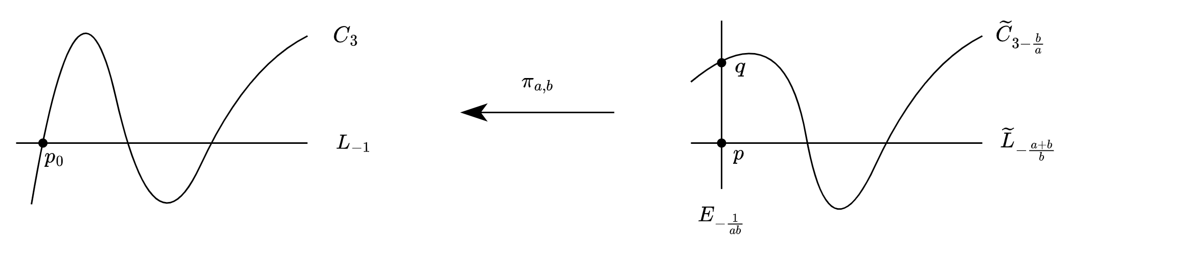
Figure 1: $(a,b)$-weighted blowup.

In the figure above, the subscripts represent the self-intersections, $E$ is the exceptional divisor of the weighted blowup and $\widetilde{C}$ and $\widetilde{L}$ are the strict transforms of $C$ and $L$, respectively.
In order to cumpute Zariski Decomposition of the divisor $\pi_{a,b}(-K_{X})-tE$, we write $\pi_{a,b}(-K_{X})-tE$ as a non-negative combination of negative divisors (See Theorem 2.12). Notice that $(\widetilde{C})^{2}>0$, so we need to find a way to write $\widetilde{C}$ as the sum of negative divisors.

4.1 Notation

As in Theorem 1.1, let $p_{0}=(x_{0},y_{0},z_{0},w_{0})\in X$ be a closed point with $w_{0}\neq 0$. Let $X_{a,b}$ be the $(a,b)$-weighted blowup of $X$ at $p_{0}$. Let $Q=T_{p_{0}}X\cap X$ be the tangent hyperplane section at $p_{0}$ defined in §3.2. Assume that $Q=L\cup C$ where $L$ is a line and $C$ is a cubic such that they intersect transversally at $p_{0}$. Let $E$ be the exceptional divisor of the weighted blowup. We assume $\frac{\sqrt{3}}{2}a\leq b\leq a$ and $\gcd(a,b)=1$. Therefore, we can rewrite $a=b+\delta$ where $\delta\in\{1,...,b-1\}$. Similarly, we can rewrite $b=\delta\cdot i+\gamma_{0}$ and $\delta=\gamma_{0}\cdot j+\gamma_{1}$ where $\gamma_{0}\in\{1,...,\delta-1\}$ and $\gamma_{1}\in\{1,...,\gamma_{0}-1\}$. Generalizing this, let $\gamma_{k}=\gamma_{k+1}\cdot j_{k+1}+\gamma_{k+2}$ where $\gamma_{k+2}\in\{1,...,\gamma_{k+1}-1\}$.

Since $\{\gamma_{k}\}$ is a decreasing sequence of natural numbers, there exists a $k_{0}\in\mathbb{N}$ where $\gamma_{k_{0}}=1$. Furthermore, we can choose $k_{0}$ such that for any other $k^{\prime}\in\mathbb{N}$ where $\gamma_{k^{\prime}}=1$, $k^{\prime}\geq k_{0}$.

Let us denote $so_{n}=\sum_{m=1}^{n}j_{2m-1}$ and $se_{n}=\sum_{m=1}^{n}j_{2m}$ and for $n=0$, $so_{0}=se_{0}=0$.

4.2 The resolution of $X_{a,b}$ followed by contractions to a weak degree 1 del Pezzo

An $(a,b)$-weighted blowup of a smooth surface has at most two quotient singularities $p$ and $q$. If $a\neq 1$, $q$ is a $\frac{1}{a}(1,c_{1})$ singularity and if $b\neq 1$, $p$ is a $\frac{1}{b}(1,d_{1})$ singularity, where $c_{1}=-b+n_{1}a$ and $d_{1}=-a+m_{1}b$, with $n_{1}=\left\lceil\frac{b}{a}\right\rceil=1$ and $m_{1}=\left\lceil\frac{a}{b}\right\rceil=2$, respectively.
Similarly, we define the following:

• $c_{2}=-a+n_{2}c_{1}$, where $n_{2}=\left\lceil\frac{a}{c_{1}}\right\rceil$ and $c_{k}=-c_{k-2}+n_{k}c_{k-1}$ where $n_{k}=\left\lceil\frac{c_{k-2}}{c_{k-1}}\right\rceil$.

• $d_{2}=-b+m_{2}d_{1}$, where $m_{2}=\left\lceil\frac{b}{d_{1}}\right\rceil$ and $d_{k}=-d_{k-2}+m_{k}d_{k-1}$ where $m_{k}=\left\lceil\frac{d_{k-2}}{d_{k-1}}\right\rceil$.

The resolution of these singularities is analogous to the Euclidean algorithm. The resolution of the singularity $p$ is achieved for some $i_{0}\in\mathbb{N}$ such that $d_{i_{0}}=1$ and similarly for $q$, the resolution will be complete when for some $j_{0}\in\mathbb{N}$ we get $c_{j_{0}}=1$.

Remark 4.1.

Each $d_{k}$ can be represented as $d_{k}=\mu_{k}b+\lambda_{k}a$. Similarly, each $c_{k}$ can be represented as $c_{k}=\beta_{k}b+\alpha_{k}a$. Notice that the property $\bullet_{k}=-\bullet_{k-2}+m_{k}\cdot\bullet_{k-1}$ also holds for the coefficients $\mu_{k}$ and $\lambda_{k}$, and $\bullet_{k}=-\bullet_{k-2}+n_{k}\cdot\bullet_{k-1}$ holds for $\alpha_{k}$ and $\beta_{k}$.

From now on, we assume neither $a$ nor $b$ are equal to $1$. If this is not the case, it is enough to omit the singularity that corresponds to that weight. We present an algorithm to determine the resolution of $X_{a,b}$. It can be achieved by repeatedly blowing up the singularities.

Resolution of $p$.

Let $\sigma_{1}:\hat{X}_{a,b}\to X_{a,b}$ be the blowup of $X_{a,b}$ at $p_{0}$. Let $E^{1}$ be the exceptional divisor and let $\hat{L}$, $\hat{C}$ and $\hat{E}$ be the strict transforms of $\widetilde{L}$, $\widetilde{C}$ and $E$ respectively. Since $p_{0}$ is a $\frac{1}{b}(1,d_{1})$ singularity, $(E^{1})^{2}=-\frac{b}{d_{1}}$, $\sigma_{1}^{*}(\widetilde{L})\cong\hat{L}+\frac{d_{1}}{b}E^{1}$, $\sigma_{1}^{*}(\widetilde{C})\cong\hat{C}$ and $\sigma_{1}^{*}(E)\cong\hat{E}+\frac{1}{b}E^{1}$. Therefore, we get the following self-intersections:

$$(\hat{L})^{2}=\left(\sigma_{1}^{*}(\widetilde{L})-\frac{d_{1}}{b}E^{(1)}\right)^{2}=(\sigma_{1}^{*}(\widetilde{L}))^{2}+\left(\frac{d_{1}}{b}E^{(1)}\right)^{2}=-\frac{a+b}{b}-\frac{d_{1}}{b}=-(1+m_{1})$$

$$(\hat{E})^{2}=\left(\sigma_{1}^{*}({E})-\frac{1}{b}E^{(1)}\right)^{2}=(\sigma_{1}^{*}(E))^{2}+\left(\frac{1}{b}E^{(1)}\right)^{2}=-\frac{1}{ab}-\frac{1}{bd_{1}}=-\frac{m_{1}}{ad_{1}}=-\frac{\mu_{1}}{ad_{1}}$$

$$(\hat{C})^{2}=\left(\sigma_{1}^{*}(\widetilde{C})\right)^{2}=3-\frac{b}{a}.$$

After this new blowup, if $d_{1}=1$, $\hat{X}_{a,b}$ will only have a singularity left and we continue with the resolution of $q$. On the other hand, if $d_{1}\neq 1$, $\hat{X}_{a,b}$ has a singularity of type $\frac{1}{d_{1}}(1,d_{2})$ (as well as $q$) in the intersection of $E^{(1)}$ with $\hat{E}$ and we iterate the process by blowing it up. Denote this new blow-up by $\sigma_{2}:\dot{X}_{a,b}\to\hat{X}_{a,b}$. Let $E^{(2)}$ the exceptional divisor of the $\sigma_{2}$ blowup, where $(E^{(2)})^{2}=-\frac{d_{1}}{d_{2}}$. Let $\dot{E}^{(1)}$ and $\dot{E}$ be the strict transforms of $E^{(1)}$ and $\hat{E}$ respectively. We get the following self-intersections:

$$(\dot{E}^{(1)})^{2}=\left(\sigma_{2}^{*}(E^{(1)})-\frac{d_{2}}{d_{1}}E^{(2)}\right)^{2}=(\sigma_{2}^{*}(E^{(1)}))^{2}+\left(\frac{d_{2}}{d_{1}}E^{(2)}\right)^{2}=-\frac{b}{d_{1}}-\frac{d_{2}}{d_{1}}=-m_{2}$$

$$(\dot{E})^{2}=\left(\sigma_{1}^{*}(\hat{E})-\frac{1}{d_{1}}E^{(2)}\right)^{2}=(\sigma_{1}^{*}(\hat{E}))^{2}+\left(\frac{1}{d_{1}}E^{(2)}\right)^{2}=-\frac{m_{1}}{ad_{1}}-\frac{1}{d_{1}d_{2}}$$

$$\;\;\;\;\;\;\;=-\frac{(m_{1}m_{2}-1)d_{1}}{ad_{1}d_{2}}=-\frac{m_{1}m_{2}-1}{ad_{2}}=-\frac{\mu_{2}}{ad_{2}}.$$

Since $\gcd(a,b)=1$, by the Euclidean algorithm there exists an $i_{0}\in\mathbb{N}$ such that $d_{i_{0}}=1$. Therefore, the resolution of $p$ is achieved after $i_{0}$ steps. Let us denote $f_{p}:\check{X}_{a,b}\to X_{a,b}$ the resolution of $p$ defined as $f_{p}=\sigma_{1}\circ\sigma_{2}\circ\cdots\circ\sigma_{i_{0}-1}\circ\sigma_{i_{0}}$. Let $\check{E}^{(k)}$, $\check{E}$, $\check{L}$, and $\check{C}$ be the strict transforms of our divisors at the $i_{0}$-th blowup. Then, we have the following self-intersections:

$$(\check{E}^{(k)})^{2}=-m_{k+1}\text{ for }k=1,...,i_{0}-1,\;\;\;\;(E^{i_{0}})^{2}=-d_{i_{0}-1}$$

$$(\check{E})^{2}=-\frac{\mu_{i_{0}}}{a},\;\;\;\;(\check{L})^{2}=-(1+m_{1}),\;\;\;\;(\check{C})^{2}=3-\frac{b}{a}.$$

Remark 4.2.

By induction one can prove that $(\check{E})^{2}=-\frac{\mu_{i_{0}}}{a}$:

Assume it is true for the $k$-th blowup, $E^{2}=-\frac{\mu_{k}}{ad_{k}}$. Let us check that it holds for the ($k+1$)-th blowup.

$$E^{2} =-\frac{\mu_{k}}{ad_{k}}-\frac{1}{d_{k}d_{k+1}}=-\frac{\mu_{k}(-d_{k-1}+m_{k+1}d_{k})+a}{ad_{k}d_{k+1}}=-\frac{a-\mu_{k}d_{k-1}+\mu_{k}m_{k+1}d_{k}}{ad_{k}d_{k+1}}.$$

It is enough to show that $a-\mu_{k}d_{k-1}=-\mu_{k-1}d_{k}$. Notice that we know $a=\mu_{k-1}d_{k-2}-\mu_{k-2}d_{k-1}$.

$$\mu_{k}d_{k-1}-\mu_{k-1}d_{k}=(-\mu_{k-2}+m_{k}\mu_{k-1})d_{k-1}-\mu_{k-1}(-d_{k-2}+m_{k}d_{k-1})=\mu_{k-1}d_{k-2}-\mu_{k-2}d_{k-1}=a$$

Therefore, we get $E^{2}=-\frac{\mu_{k+1}}{ad_{k+1}}$. In particular, since $d_{i_{0}}=1$, $(\check{E})^{2}=-\frac{\mu_{i_{0}}}{a}$.

The values of $i_{0}$, $d_{i_{0}-1}$, and $m_{k}$ can be specified using the notation of Subsection 4.1. We have two possibilities:

• If $k_{0}=2n_{0}$,

  $$i_{0}=i+so_{n_{0}}\;\text{ and }\;\left(\check{E}^{\left(i+so_{n}+k\right)}\right)^{2}=-m_{\left(i+so_{n}+k+1\right)}=\left\{\begin{array}[]{ll}-\left(j_{2n}+2\right)&\text{ if }k=0,\\ -2&\text{ Otherwise. }\end{array}\right.$$

  $$(\check{E}^{i_{0}})^{2}=-d_{i_{0}-1}=-(j_{2n_{0}}+1).$$

• If $k_{0}=2n_{0}+1$,

  $$i_{0}=i+so_{n_{0}+1}-1\;\text{ and }\;\left(\check{E}^{\left(i+so_{n}+k\right)}\right)^{2}=-m_{\left(i+so_{n}+k+1\right)}=\left\{\begin{array}[]{ll}-\left(j_{2n}+2\right)&\text{ if }k=0,\\ -2&\text{ Otherwise. }\end{array}\right.$$

  $$(\check{E}^{i_{0}})^{2}=-d_{i_{0}-1}=-2.$$

Resolution of $q$.

Let $\tau_{1}:\overset{\cdot\cdot}{X}_{a,b}\to\check{X}_{a,b}$ be the blowup of $\check{X}_{a,b}$ at $q$. Let $F^{(1)}$ be the exceptional divisor and $\overset{\cdot\cdot}{L}$, $\overset{\cdot\cdot}{C}$ $\overset{\cdot\cdot}{E^{k}}$ and $\overset{\cdot\cdot}{E}$ be the strict transforms of $\check{L}$, $\check{C}$, $\check{E}^{k}$ and $\check{E}$ respectively. Since $q$ is a $\frac{1}{a}(1,c_{1})$, $(F^{(1)})^{2}=-\frac{a}{c_{1}}$. Also, since $q$ is in the intersection between $\check{E}$ and $\check{C}$, their strict transforms are not isomorphic to the pullbacks: $\tau_{1}^{*}(\check{C})\cong\overset{\cdot\cdot}{C}+\frac{c_{1}}{a}F^{(1)}$ and $\tau_{1}^{*}(\check{E})\cong\overset{\cdot\cdot}{E}+\frac{1}{a}F^{(1)}$. Therefore, these are the self-intersections that change:

$$(\overset{\cdot\cdot}{C})^{2}=\left(\tau_{1}^{*}(\check{C})-\frac{c_{1}}{a}F^{(1)}\right)^{2}=(\tau_{1}^{*}(\check{C}))^{2}+\left(\frac{c_{1}}{a}F^{(1)}\right)^{2}=3-\frac{b}{a}-\frac{c_{1}}{a}=3-n_{1}$$

$$(\overset{\cdot\cdot}{E})^{2}=\left(\tau_{1}^{*}(\check{E})-\frac{1}{a}F^{(1)}\right)^{2}=(\tau_{1}^{*}(\check{E}))^{2}+\left(\frac{1}{a}F^{(1)}\right)^{2}=-\frac{\mu_{i_{0}}}{a}-\frac{1}{ac_{1}}=-\frac{n_{1}\mu_{i_{0}}+\lambda_{i_{0}}}{c_{1}}$$

$$\;\;\;\;\;\;\;=-\frac{\alpha_{1}\mu_{i_{0}}-\beta_{1}\lambda_{i_{0}}}{c_{1}}.$$

After this blowup, if $c_{1}=1$, $\overset{\cdot\cdot}{X}_{a,b}$ is smooth and it is the resolution. On the other hand, if $c_{1}\neq 1$, $\overset{\cdot\cdot}{X}_{a,b}$ has a singularity of type $\frac{1}{c_{1}}(1,c_{2})$ in the intersection of $F^{(1)}$ and $\overset{\cdot\cdot}{E}$, and we iterate the process by blowing it up, with the blow up denoted by $\tau_{2}:\overset{\cdots}{X}_{a,b}\to\overset{\cdot\cdot}{X}_{a,b}$. Let $F^{(2)}$ the exceptional divisor of the $\tau_{2}$ blowup, where $(F^{(2)})^{2}=-\frac{c_{1}}{c_{2}}$. Let $\overset{\cdots}{F^{(1)}}$ and $\overset{\cdots}{E}$ be the strict transforms of $F^{(1)}$ and $\overset{\cdot\cdot}{E}$, respectively. We get the following self-intersections:

$$\left(\overset{\cdots}{F}^{(1)}\right)^{2}=\left(\tau_{2}^{*}(F^{(1)})-\frac{c_{2}}{c_{1}}F^{(2)}\right)^{2}=(\tau_{2}^{*}(F^{(1)}))^{2}+\left(\frac{c_{2}}{c_{1}}F^{(2)}\right)^{2}=-\frac{a}{c_{1}}-\frac{c_{1}}{c_{2}}=-n_{2}$$

$$(\overset{\cdots}{E})^{2}=\left(\tau_{1}^{*}(\check{E})-\frac{1}{a}F^{(1)}\right)^{2}=(\tau_{1}^{*}(\check{E}))^{2}+\left(\frac{1}{c_{1}}F^{(1)}\right)^{2}=-\frac{\mu_{i_{0}}}{c_{1}}-\frac{1}{ac_{1}}=-\frac{\alpha_{1}\mu_{i_{0}}-\beta_{1}\lambda_{i_{0}}}{c_{1}}-\frac{1}{c_{1}c_{2}}$$

$$\;\;\;\;\;\;\;\;=-\frac{\alpha_{2}\mu_{i_{0}}-\beta_{2}\lambda_{i_{0}}}{c_{2}}$$

Since $\gcd(a,b)=1$ by the Euclidean algorithm there exist $j_{0}\in\mathbb{N}$ such that $c_{j_{0}}=1$. Therefore, the resolution of $q$ is achieved after $j_{0}$ steps. Let us denote $f_{q}:\overline{X}_{a,b}\to\check{X}_{a,b}$ the resolution of $q$ defined as $f_{q}=\tau_{1}\circ\tau_{2}\circ\cdots\circ\tau_{j_{0}-1}\circ\tau_{j_{0}}$. Let $\overline{F}^{(k)}$, $\overline{E}^{(s)}$, $\overline{E}$, $\overline{L}$ and $\overline{C}$ be the strict transforms of our divisors after the $(i_{0}+j_{0})$-th blowup. Then, we have the following self-intersections:

$$(\overline{F}^{(k)})^{2}=-n_{k+1}\text{ for }k=1,...,j_{0}-1,\;\;\;\;(\overline{F}^{(j_{0})})^{2}=-c_{j_{0}-1}$$

$$(\overline{E})^{2}=-1,\;\;\;\;(\overline{C})^{2}=3-n_{1}.$$

Remark 4.3.

Notice that the self-intersections of $\overline{E}^{k}$ and $\overline{L}$ are the same as their images through $f_{q}$. In order to prove that $(\overline{E})^{2}=-1$, first we see that in the $(i_{0}+k)$-th blowup, $(E)^{2}=-\frac{\alpha_{k}\mu_{i_{0}}-\beta_{k}\lambda_{i_{0}}}{c_{k}}$. And then we see that $\alpha_{j_{0}}\mu_{i_{0}}-\beta_{j_{0}}\lambda_{i_{0}}=1$.
As before, by induction on k, assume it is true for the $i_{0}+k$-th blowup. Then let us see that it also holds for the $k+1$-th.

$$(E)^{2} =-\frac{\alpha_{k}\mu_{i_{0}}-\beta_{k}\lambda_{i_{0}}}{c_{k}}-\frac{1}{c_{k}c_{k+1}}=-\frac{(\alpha_{k}\mu_{i_{0}}-\beta_{k}\lambda_{i_{0}})c_{k+1}+1}{c_{k}c_{k+1}}$$

$$=-\frac{(\alpha_{k}\mu_{i_{0}}-\beta_{k}\lambda_{i_{0}})(-c_{k-1}+n_{k+1}c_{k})+1}{c_{k}c_{k+1}}$$

$$=-\frac{1-(\alpha_{k}\mu_{i_{0}}-\beta_{k}\lambda_{i_{0}})c_{k-1}+(\alpha_{k}\mu_{i_{0}}-\beta_{k}\lambda_{i_{0}})n_{k+1}c_{k}}{c_{k}c_{k+1}}$$

So it is enough to prove that $1-(\alpha_{k}\mu_{i_{0}}-\beta_{k}\lambda_{i_{0}})c_{k-1}=(\alpha_{k-1}\mu_{i_{0}}-\beta_{k-1}\lambda_{i_{0}})c_{k}$.

$$(\alpha_{k}\mu_{i_{0}}-\beta_{k}\lambda_{i_{0}})c_{k-1}+(\alpha_{k-1}\mu_{i_{0}}-\beta_{k-1}\lambda_{i_{0}})c_{k}$$

$$=((-\alpha_{k-2}+n_{k}\alpha_{k-1})\mu_{i_{0}}-(-\beta_{k-2}+m_{k}\beta_{k-1})\lambda_{i_{0}})c_{k-1}+(\alpha_{k-1}\mu_{i_{0}}-\beta_{k-1}\lambda_{i_{0}})(-c_{k-2}+n_{k}c_{k-1})$$

$$=(\alpha_{k-1}\mu_{i_{0}}-\beta_{k-1}\lambda_{i_{0}})c_{k}=1$$

Where for the first equation we use that $1=(\alpha_{k-1}\mu_{i_{0}}-\beta_{k-1}\lambda_{i_{0}})c_{k-2}+(\alpha_{k-2}\mu_{i_{0}}-\beta_{k-2}\lambda_{i_{0}})c_{k-1}$. Therefore, we get, $(E)^{2}=-\frac{\alpha_{k}\mu_{i_{0}}-\beta_{k}\lambda_{i_{0}}}{c_{k}}$. And in particular, since $c_{j_{0}}=1$ in the last blowup we get $(\overline{E})^{2}=-(\alpha_{j_{0}}\mu_{i_{0}}-\beta_{j_{0}}\lambda_{i_{0}})$.
Finally, we need to show that $\alpha_{j_{0}}\mu_{i_{0}}-\beta_{j_{0}}\lambda_{i_{0}}=1$. We know by definition that $\alpha_{j_{0}}a+\beta_{j_{0}}b=b\mu_{i_{0}}+a\lambda_{i_{0}}=1$. So, $a=n(\mu_{i_{0}}-\beta_{j_{0}})$, $b=n(\alpha_{j_{0}}-\lambda_{i_{0}})$. However, by the choice of $\mu_{i_{0}}$, $\lambda_{i_{0}}$, $\beta_{j_{0}}$ and $\alpha_{j_{0}}$, we conclude $n=1$. Then, since $\lambda_{i_{0}}=\alpha_{j_{0}}-b$, $\mu_{i_{0}}=\beta_{j_{0}}+a$,

$$(\overline{E})^{2}=-(\alpha_{j_{0}}\mu_{i_{0}}-\beta_{j_{0}}\lambda_{i_{0}})=-1$$

The values of $j_{0}$, $c_{j_{0}-1}$ and $n_{k}$ can be specified using the notation in §4.1. We have two possibilities:

• If $k_{0}=2n_{0}$,

  $$j_{0}=j+se_{n_{0}}\;\text{ and }\;\left(\overline{F}^{\left(j+se_{n}+k\right)}\right)^{2}=-n_{\left(j+se_{n}+k+1\right)}=\left\{\begin{array}[]{ll}-\left(j_{2n+1}+2\right)&\text{ if }k=1,\\ -2&\text{ Otherwise. }\end{array}\right.$$

  $$(\overline{F}^{(1)})^{2}=-n_{2}=-(i+2),\;\;\;\;(F^{(j_{0})})^{2}=-c_{j_{0}-1}=-2.$$

  In the following pictures, we can see all the divisors involved in the resolution of the singularities $p$ and $q$ when $k_{0}=2n_{0}$. Notice that the subscripts represent the self-intersection numbers.

  

• If $k_{0}=2n_{0}+1$,

  $$j_{0}=j+se_{n_{0}}+1\;\text{ and }\;\left(\overline{F}^{\left(j+se_{n}+k\right)}\right)^{2}=-n_{\left(j+se_{n}+k+1\right)}=\left\{\begin{array}[]{ll}-\left(j_{2n+1}+2\right)&\text{ if }k=1,\\ -2&\text{ Otherwise. }\end{array}\right.$$

  $$(\overline{F}^{(1)})^{2}=-n_{2}=-(i+2),\;\;\;\;(F^{(j_{0})})^{2}=-c_{j_{0}-1}=-(j_{2n_{0}+1}+1).$$

  In the following picture, we can see all the divisors involved in the resolution of the singularities $p$ and $q$ when $k_{0}=2n_{0}+1$. The subscripts represent the self-intersection numbers.

  

Notice that in both cases, we can contract $(-1)$-curves until we get a weak del Pezzo degree one surface:

• For $k=2n_{0}$:

  • Contract $\overline{E}$,

  • Contract $F^{(j+se_{n_{0}})}$,…, $\overline{F}^{(j+2+se_{n_{0}-1})}$ ($j_{2n_{0}}-1$ contractions).

  • Contract $\overline{E}^{(i+so_{n_{0}})}$,…, $\overline{E}^{(i+1+so_{n_{0}-1})}$ ($j_{2n_{0}-1}$ contractions).

  • Contract $\overline{F}^{(j+1+se_{n_{0}-1})}$,…, $\overline{F}^{(j+2+se_{n_{0}-1})}$ ($j_{2n_{0}-2}$ contractions).
    ⋮

  • Contract $\overline{E}^{(i+j_{1})}$,…, $\overline{E}^{(i+1)}$ ($j_{1}$ contractions).

  • Contract $\overline{F}^{(j+1)}$,…, $\overline{F}^{(2)}$ ($j$ contractions).

  • Contract $\overline{E}^{(i)}$,…, $\overline{E}^{(1)}$ ($i$ contractions).

• For $k=2n_{0}+1$:

  • Contract $\overline{E}$,

  • Contract $\overline{E}^{(i+so_{n_{0}+1}-1)}$,…, $\overline{E}^{(i+1+so_{n_{0}})}$ ($j_{2n_{0}+1}-1$ contractions).

  • Contract $F^{(j+se_{n_{0}}+1)}$,…, $\overline{F}^{(j+2+se_{n_{0}-1})}$ ($j_{2n_{0}}$ contractions).

  • Contract $\overline{E}^{(i+so_{n_{0}})}$,…, $\overline{E}^{(i+1+so_{n_{0}-1})}$ ($j_{2n_{0}-1}$ contractions).
    ⋮

  • Contract $\overline{E}^{(i+j_{1})}$,…, $\overline{E}^{(i+1)}$ ($j_{1}$ contractions).

  • Contract $\overline{F}^{(j+1)}$,…, $\overline{F}^{(2)}$ ($j$ contractions).

  • Contract $\overline{E}^{(i)}$,…, $\overline{E}^{(1)}$ ($i$ contractions).

In total, we contract $i_{0}+j_{0}=i+j+\sum_{k=1}^{k_{0}}j_{k}$ (-1)-curves in both cases. Let $g:\overline{X}_{a,b}\to\mathbf{X}$ the composition of all the contractions. The picture at the end is:

Where $\overset{\circ}{F^{(1)}}=g(\overline{F^{(1)}})$, $\overset{\circ}{C}=g(\overline{C})$ and $\overset{\circ}{L}=g(\overline{L})$. We see now that this $\mathbf{X}$ is a weak del Pezzo surface of degree 1.

Proposition 4.4.

The surface $\mathbf{X}$ is a weak del Pezzo surface of degree 1.

Proof.

Notice that at the beginning, before the weighted blowup, we have $-K_{X}\sim\frac{1}{2}(L+C)$, ($L$ and $C$ defined as in Theorem 1.1). With each blowup we do for the resolution, we get an exceptional divisor, as we saw above, and these divisors are added with a nonpositive coefficient to the equivalence class of the anticanonical. For instance, with the weighted blowup we get

$$-K_{X_{a,b}}\sim\pi^{*}(-K_{S})-(a+b-1)E\sim\frac{1}{2}(\widetilde{L}+\widetilde{C})-\frac{a+b-2}{2}E.$$

Notice that the coefficients of the strict transforms of the existing divisors do not change and do not change in the successive ordinary blowups either. The same thing happens when we contract exceptional curves, the coefficients of the remaining exceptional curves do not change in the process. Therefore, to prove that $(-K_{\mathbf{X}})^{2}=1$. We need to find the coefficient $e$ of $\overset{\circ}{F^{(1)}}$ in $-K_{\mathbf{X}}\sim\frac{1}{2}(\overset{\circ}{L}+\overset{\circ}{C})+e\overset{\circ}{F^{(1)}}$.
We got $F^{(1)}$, with the first blowup of the singular point $q\sim\frac{1}{a}(1,c_{1})$, where $c_{1}=-b+a$.
Therefore, after the ordinary blowup at $q=C\cap E$, $\sigma:Y\to X_{a,b}$, (we are abusing notation here since this is not the exact same order of resolution we used above, but the coefficient of $F^{(1)}$ still is the same since it is independent of the order of the blowup), we get the following:

$$\begin{array}[]{rl}-K_{Y}\sim&\sigma^{*}\left(-K_{X_{a,b}}\right)+\frac{a-(c_{1}+1)}{a}F^{1}\\ \sim&\frac{1}{2}(\bar{L}+\bar{C})-\frac{a+b-2}{2}\bar{E}+\left(-\frac{a+b-2}{2a}+\frac{c_{1}}{2a}+\frac{a-(c_{1}+1)}{a}\right)F^{1}\\ \sim&\frac{1}{2}(\bar{L}+\bar{C})-\frac{a+b-2}{2}\bar{E}-\frac{c_{1}+b-a}{2a}F^{(1)}.\end{array}$$

However, notice that $e=\frac{c_{1}+b-a}{2a}=0$. So we have that, $(-K_{\mathbf{X}})^{2}=\left(\frac{1}{2}(\overset{\circ}{L}+\overset{\circ}{C})\right)^{2}=1$. ∎

Remark 4.5.

In a weak del Pezzo surface of degree 1, we have a birational involution called the Bertini involution, $\iota$. As in the proof of Lemma 2.15 in [ACC⁺23], the linear system $|-2K_{\mathbf{X}}|$ gives a morphism $\mathbf{X}\to\mathbb{P}(1,1,2)$ with the following Stein factorization:

where $\upsilon$ is a contraction of all $(-2)$-curves in the surface $\mathbf{X}$ (if any), and $\omega$ is a double cover branched over the union of a sextic curve in $\mathbb{P}(1,1,2)$ and the singular points of $\mathbb{P}(1,1,2)$. Notice that $\mathbf{X}$ is smooth if and only if $-K_{\mathbf{X}}$ is ample, and in that case, $\upsilon$ is an isomorphism. Furthermore, if the divisor $-K_{\mathbf{X}}$ is not ample, then the surface $\mathbf{X}$ contains at most four (-2)-curves. The double cover $\widetilde{\mathbf{X}}\to\mathbb{P}(1,1,2)$ induces an involution $\iota\in\operatorname{Aut}(\mathbf{X})$ known as the Bertini involution.
For detailed equations of the Bertini involution, check [Moo43].

Let $\overset{\circ}{D}=\iota(\overset{\circ}{F^{(1)}})$, and with this involution it is straightforward to check that

$$\overset{\circ}{F^{(1)}}+\overset{\circ}{D}+\overset{\circ}{L}\sim-2K_{\mathbf{X}}.$$

Lemma 4.6.

Let $\overset{\circ}{D}$, $\overset{\circ}{F^{(1)}}$ and $\overset{\circ}{L}$ described as above. Then they do not intersect at the same point.

Proof.

In this proof, we have to take into account several things. Notice that in $\widetilde{\mathbf{X}}$, $\upsilon(\overset{\circ}{F^{(1)}})\cdot\upsilon(\overset{\circ}{D})=3$ and both of them contain the singular point coming from the contraction of $\overset{\circ}{L}$. Then, after the blowup of the singular point at $\widetilde{\mathbf{X}}$, we recover $\overset{\circ}{L}$ again, and since $\overset{\circ}{F^{(1)}}+\overset{\circ}{D}+\overset{\circ}{L}\sim-2K_{\mathbf{X}}$ the intersections change as follows:

$$\overset{\circ}{F^{(1)}}\cdot\overset{\circ}{D}=2,\;\;\;\overset{\circ}{F^{(1)}}\cdot\overset{\circ}{L}=\overset{\circ}{L}\cdot\overset{\circ}{D}=1.$$

This implies that $\overset{\circ}{F^{(1)}}\cap\overset{\circ}{D}\cap\overset{\circ}{L}=0$. ∎

As a consequence, we have the following proposition:

Proposition 4.7.

Let $\widetilde{D}=(f_{p}\circ f_{q})(g^{*}(\overset{\circ}{D}))$ be a generator of the effective cone of $X_{a,b}$ when $3a<4b$. Then, we can rewrite $C$ in terms of the generators of the effective cone of $X_{a,b}$, such that $\widetilde{C}=\widetilde{D}+bE_{a,b}$ and $(\widetilde{D})^{2}=3-\frac{4b}{a}<0$.

Proof.

The idea of this proof is to take the equivalence $\overset{\circ}{C}\sim\overset{\circ}{F^{1}}+\overset{\circ}{D}$ in $\mathbf{X}$, and following the inverse process get an equivalence for $\widetilde{C}$ in $X_{a,b}$ in terms of $\widetilde{D}$ and $E_{a,b}$. Let $e_{k}$ and $f_{k}$ be the coefficient of $E^{k}$ and $F^{k}$, respectively, in the equivalence class of $C$. Define $e$ to be the final coefficient of $E_{a,b}$. Notice that if $k=2n_{0}$, $e=e_{i+so_{n_{0}}}+f_{j+se_{n_{0}}}$, otherwise $e=e_{i+so_{n_{0}+1}-1}+f_{j+se_{n_{0}}+1}$. In addition, we know for the sequence of blowups that for $n\geq 0$

$$\begin{array}[]{rlr}e_{i+so_{n}+k}=&e_{i+so_{n}}+k\cdot f_{j+se_{n}+1}&\text{for }k=1,...,j_{2n+1},\\ f_{j+se_{n}+k+1}=&k\cdot e_{i+so_{n+1}}+f_{j+se_{n}+1}&\text{for }k=1,...,j_{2n+2}.\end{array}$$

Now let us rewrite $b$ in terms of $i$, $j$, and $j_{k}$ using notation as in §4.1.

$$\begin{array}[]{rl}b=&\delta\cdot i+\gamma_{0}=\delta\cdot e_{i}+\gamma_{0}=\gamma_{0}(e_{i}\cdot j+1)+\gamma_{1}\cdot e_{i}=\gamma_{0}\cdot f_{j+1}+\gamma_{1}\cdot e_{i}=\\ =&\gamma_{1}(j_{1}\cdot f_{j+1}+e_{i})+\gamma_{2}\cdot f_{j+1}=\gamma_{1}\cdot e_{i+so_{1}}+\gamma_{2}\cdot f_{j+1}=...=\\ =&\gamma_{2n_{0}-2}f_{j+se_{n_{0}-1}+1}+\gamma_{2n_{0}-1}e_{i+se_{n_{0}-1}}=\gamma_{2n_{0}-1}e_{i+so_{n_{0}}}+\gamma_{2n_{0}}f_{j+se_{n_{0}-1}+1}\end{array}$$

Here we have two different cases.

• If $k_{0}=2n_{0}$, notice that, $\gamma_{2n_{0}-1}=j_{2n_{0}}$ and $\gamma_{2n_{0}}=1$. Therefore,

  $$b=j_{2n_{0}}e_{i+so_{n_{0}}}+f_{j+se_{n_{0}-1}+1}=f_{j+se_{n_{0}}}+e_{i+so_{n_{0}}}=e.$$

• If $k_{0}=2n_{0}+1$, notice that $\gamma_{2n_{0}}=j_{2n_{0}+1}$ and $\gamma_{2n_{0}+1}=1$. Therefore,

  $$b=j_{2n_{0}+1}f_{j+se_{n_{0}}+1}+e_{i+so_{n_{0}}}=e_{i+so_{n_{0}+1}-1}+f_{j+se_{n_{0}}+1}=e.$$

In both cases, as desired, we obtain $e=b$. Therefore, after all the contractions, we get $\widetilde{C}\sim D+b\cdot E_{a,b}$. To compute the self-intersection of $D$:

$$(\widetilde{D})^{2}=(\widetilde{C}-bE)^{2}=\widetilde{C}^{2}-2b\widetilde{C}\cdot E+b^{2}E^{2}=3-\frac{b}{a}-\frac{2b}{a}-\frac{b}{a}=3-\frac{4b}{a}<0\;\;\Leftrightarrow\;\;3a<4b.$$

∎

5 Proof of the Main Theorem

In the previous section, we prepared all ingredients to prove the Main Theorem. Now, we divide this proof into two results:

Theorem 5.1.

Let $X\subset\mathbb{P}(1,1,1,2)$ be a smooth del Pezzo surface of degree 2 and let $p_{0}=(x_{0},y_{0},z_{0},w_{0})\in X$ be a closed point with $w_{0}\neq 0$. Let $Q=T_{p_{0}}\cap X$ be the tangent hyperplane section. Assume that $Q=L\cup C$ where $L$ is a line, $Q$ is a cubic, and they intersect transversally at $p_{0}$. Then $\delta_{p_{0}}(X)\leq\frac{6}{71}(11+8\sqrt{3})$.

Proof.

For each $a,b>0$, let $\nu_{a,b}$ be the quasi-monomial valuation over $x\in X$ defined by $\nu_{a,b}(u)=a$ and $\nu_{a,b}(v)=b$. We need to identify the minimizer of $\frac{A_{S}(\nu_{a,b})}{S_{S}(\nu_{a,b})}$. In order to do this, choose coprime integers $a,b>0$ and let $\pi:Y=Y_{a,b}\to X$ be the weighted blow up at $p_{0}$ with $\operatorname{wt}(u)=a$ and $\operatorname{wt}(v)=b$. Let $E$ be the exceptional divisor and let $\widetilde{L}$, and $\widetilde{C}$ be the strict transforms of $L$ and $C$, respectively. Assume that $\frac{\sqrt{3}}{2}a<b<a$.

By definition, $\overline{L}=\pi^{*}(L)=\widetilde{L}+m_{L}E$ and $\overline{C}=\pi^{*}(C)=\widetilde{C}+m_{C}E$ where in our case $m_{L}=\operatorname{mult}_{p_{0}}L=a$, $m_{C}=\operatorname{mult}_{p_{0}}C=b$, $E^{2}=-\frac{1}{ab}$ So we get, $(\widetilde{L})^{2}=-\frac{a+b}{b}$, $(\widetilde{C})^{2}=3-\frac{b}{a}$, $(\widetilde{L})\cdot E=\frac{1}{b}$, $(\widetilde{C})\cdot E=\frac{1}{a}$, and $\widetilde{C}\cdot\widetilde{L}=2$.

As we saw in the previous section, we have, $-K_{S}\sim\frac{1}{2}Q=\frac{1}{2}(L+C)$. Using this and Lemma 4.7, the stable base locus of

$$\pi^{*}(-K_{S})-tE\sim\frac{1}{2}\left(\widetilde{L}+\widetilde{C}\right)+\left(\frac{a+b}{2}-t\right)E\sim\frac{1}{2}\left(\widetilde{L}+\widetilde{D}\right)+\left(\frac{a+2b}{2}-t\right)E$$

is contained in $\widetilde{D}\cap\widetilde{L}$ for all $0\leq t\leq\frac{a+2b}{2}$ and we have the following Zariski decomposition

$$N(\pi^{*}(-K_{S})-tE)=\left\{\begin{array}[]{ll}0&0\leq t\leq b,\\ \frac{t-b}{a+b}\widetilde{L}&b<t\leq\frac{a(3a+4b)}{3a+2b},\\ \frac{3t(2b-a)-4b^{2}}{4b^{2}-3a^{2}}\widetilde{L}+\frac{t(3a+2b)-a(3a+4b)}{4b^{2}-3a^{2}}\widetilde{D}&\frac{a(3a+4b)}{3a+2b}<t\leq\frac{a+2b}{2},\end{array}\right.$$

and

$$P(\pi^{*}(-K_{S})-tE)=\left\{\begin{array}[]{ll}\frac{1}{2}\left(\widetilde{L}+\widetilde{D}\right)+\left(\frac{a+2b-2t}{2}\right)E&0\leq t\leq b\\ \frac{a+3b-2t}{2(a+b)}\widetilde{L}+\frac{1}{2}\widetilde{D}+\left(\frac{a+2b-2t}{2}\right)E&b<t\leq\frac{a(3a+4b)}{3a+2b}\\ \frac{3t(2b-a)(a+2b_{2}t)}{2(4b^{2}-3a^{2})}\widetilde{L}+\frac{(3a+2b)(a+2b-2t)}{2(4b^{2}-3a^{2})}\widetilde{D}+\left(\frac{a+2b-2t}{2}\right)E&\frac{a(3a+4b)}{3a+2b}<t\leq\frac{a+2b}{2}\end{array}\right.$$

Then, by [BFJ09, Theorem B, Example 4.7] and [LM09, Corollary C], we know that

$$\operatorname{vol}_{Y|E}(-\pi^{*}K_{S}-tE)=P_{\sigma}(\pi^{*}(-K_{S})-tE)\cdot E=-\frac{1}{2}\cdot\frac{d}{dt}\operatorname{vol}(-\pi^{*}K_{S}-tE)$$

Thus, we get

$$\operatorname{vol}_{Y|E}(\pi^{*}(-K_{S})-tE)=\left\{\begin{array}[]{ll}\frac{t}{ab}&0\leq t\leq b\\ \frac{a+t}{a(a+b)}&b<t\leq\frac{a(3a+4b)}{3a+2b}\\ \frac{6(a+2b-2t)}{4b^{2}-3a^{2}}&\frac{a(3a+4b)}{3a+2b}<t\leq\frac{a+2b}{2}\end{array}\right.$$

and

$$S(-K_{S};E)=\frac{2}{(-K_{S})^{2}}\int_{0}^{\infty}t\cdot\operatorname{vol}_{Y|E}(\pi^{*}(-K_{S})-tE)dt=\frac{15a^{2}+34ab+8b^{2}}{12(3a+2b)}.$$

Since $A_{S}(E)=a+b$, note that $\frac{A_{S}(\nu_{a,b})}{S_{S}(\nu_{a,b})}$ only depends on the ratio $\mu=\frac{a}{b}$, thus by continuity [BLX22, Proposition 2.4] we have

$$\frac{A_{S}(\nu_{a,b})}{S_{S}(\nu_{a,b})}=\frac{12(3\mu+2)(1+\mu)}{15\mu^{2}+34\mu+8}$$

for all $a,b\in\mathbb{R}_{+}$. It achieves its minimum for $\frac{2}{\sqrt{3}}\geq\mu\geq\frac{2}{3}$ with the value $\lambda_{0}=\frac{6}{71}(11+8\sqrt{3})$ at $\mu_{0}:=\frac{2}{\sqrt{3}}$. In particular, we have $\delta_{p_{0}}(X)\leq\lambda$. ∎

It remains to show $\delta_{p_{0}}(X)\geq\lambda$. We use the same method as in Lemma A.6 of [AZ22].

Theorem 5.2.

Let $X\subset\mathbb{P}(1,1,1,2)$ be a smooth del Pezzo surface of degree 2 and let $p_{0}=(x_{0},y_{0},z_{0},w_{0})\in X$ be a closed point with $w_{0}\neq 0$. Let $Q=T_{p_{0}}\cap X$ be the tangent hyperplane section. Assume that $Q=L\cup C$ where $L$ is a line, $C$ is a cubic, and they intersect transversally at $p_{0}$. Then $\delta_{p_{0}}(X)\geq\frac{6}{71}(11+8\sqrt{3})$.

Proof.

Choose a sequence of coprime integers $a_{m},b_{m}>0$ ($m=1,2,...$) such that $\mu_{m}:=\frac{a_{m}}{b_{m}}\to\mu_{0}$ ($m\to\infty$), where $\frac{2}{3}<\mu_{m}<\frac{2}{\sqrt{3}}$. Let $\pi_{m}:Y_{m}=Y_{a_{m},b_{m}}\to X$ be the corresponding weighted blow up and let $E_{m}$ be the exceptional divisor. Let $P_{1}^{(m)}=\widetilde{L}\cap E_{m}$, $P_{2}^{(m)}=\widetilde{D}\cap E_{m}=\widetilde{C}\cap E_{m}$ and let $W_{\overrightarrow{\cdot,\cdot}}^{E_{m}}$ be the refinement by $E_{m}$ of the complete linear series associated to $-K_{S}$.

Let $\Delta_{m}=\operatorname{Diff}_{E_{m}}(0)=(1-\frac{1}{b_{m}})P_{1}^{(m)}+(1-\frac{1}{a_{m}})P_{2}^{(m)}$, $\lambda_{m}=\frac{A_{S}(E_{m})}{S(-K_{S};E_{m})}$. Now using the formula in Corollary 2.14 we know that:

$$\delta_{p}(X)\geq\min\left\{\frac{A_{S}(E_{m})}{S(-K_{S};E_{m})},\;\min_{x\in E_{m}}\frac{1-\operatorname{ord}_{x}(\Delta_{E_{m}})}{S(W_{\cdot,\cdot}^{E_{m}};x)}\right\}$$

We already computed the minimum of $\frac{A_{S}(E_{m})}{S(-K_{S};E_{m})}$ in Theorem 5.1. Therefore, to finish the proof, we need the compute the other minimum. Notice that in $E_{m}$ we have two singularities, $P_{1}^{(m)}$ and $P_{2}^{(m)}$, so we have three types of points $x\in E_{m}$. Here, we denote by $P(t)$ as the positive part of the Zariski decomposition of Theorem 5.1.

• If $x=P_{1}^{(m)}$,

  $$\frac{1-\operatorname{ord}_{x}(\Delta_{E_{m}})}{S(W_{\cdot,\cdot}^{E_{m}};x)}=\frac{1-\left(1-\frac{1}{b_{m}}\right)}{S(W_{\cdot,\cdot}^{E_{m}};P_{1}^{(m)})}=\frac{12(2b_{m}+3a_{m})^{2}}{45a_{m}^{2}+60a_{m}b_{m}+44b_{m}^{2}},$$

  where

  $$\begin{split}S(W_{\cdot,\cdot}^{E_{m}};P_{1}^{(m)})&=\int_{0}^{\frac{a+2b}{2}}\left(\left(P(t)\cdot E_{m}\right)\cdot\left(N(t)\cdot E_{m}\right)_{P_{1}^{(m)}}+\frac{\left(P(t)\cdot E_{m}\right)^{2}}{2}\right)\;dt\\ &=\frac{45a_{m}^{2}+60a_{m}b_{m}+44b_{m}^{2}}{12b_{m}(2b_{m}+3a_{m})^{2}}\end{split}$$

  Now since $\mu_{m}\to\mu$ as $m\to\infty$, let us take the limit

  $$\lim_{m\to\infty}\frac{1}{b\cdot S(W_{\cdot,\cdot}^{E_{m}};P_{1}^{(m)})}=\frac{6}{47}\left(11+3\sqrt{3}\right)$$ (4)

• If $x=P_{2}^{(m)}$,

  $$\frac{1-\operatorname{ord}_{x}(\Delta_{E_{m}})}{S(W_{\cdot,\cdot}^{E_{m}};x)}=\frac{1-\left(1-\frac{1}{a_{m}}\right)}{S(W_{\cdot,\cdot}^{E_{m}};P_{2}^{(m)})}=\frac{3(2b_{m}+3a_{m})^{2}}{18a_{m}^{2}+12a_{m}b_{m}+4b_{m}^{2}},$$

  where

  $$\begin{split}S(W_{\cdot,\cdot}^{E_{m}};P_{2}^{(m)})=\frac{2(9a_{m}^{2}+6a_{m}b_{m}+2b_{m}^{2})}{3a_{m}(2b_{m}+3a_{m})^{2}}\end{split}$$

  Now since $\mu_{m}\to\mu$ as $m\to\infty$, let us take the limit

  $$\lim_{m\to\infty}\frac{1}{a\cdot S(W_{\cdot,\cdot}^{E_{m}};P_{2}^{(m)})}=\frac{6}{37}\left(8+3\sqrt{3}\right)$$ (5)

• If $x\neq P_{1}^{(m)},\,P_{2}^{(m)}$,

  $$\frac{1-\operatorname{ord}_{x}(\Delta_{E_{m}})}{S(W_{\cdot,\cdot}^{E_{m}};x)}=\frac{1}{S(W_{\cdot,\cdot}^{E_{m}};x)}=\frac{18a_{m}^{2}+12a_{m}b_{m}}{15a_{m}-2b_{m}},$$

  where

  $$\begin{split}S(W_{\cdot,\cdot}^{E_{m}};x)=\frac{15a_{m}-2b_{m}}{18a_{m}^{2}+12a_{m}b_{m}}\end{split}$$

  Now since $\mu_{m}\to\mu$ as $m\to\infty$, let us take the limit

  $$\lim_{m\to\infty}\frac{1}{S(W_{\cdot,\cdot}^{E_{m}};x)}=\frac{12}{37}\left(8+3\sqrt{3}\right)$$ (6)

  If we put it all together, we get that

  $$\delta_{p}(X)\geq\min\left\{\lambda,\eqref{P1},\eqref{P2},\eqref{genx}\right\}=\lambda=\frac{6}{71}(11+8\sqrt{3})$$

∎

This concludes the proof of the Main Theorem 1.1.

School of Mathematical Sciences, University of Nottingham, Nottingham, NG7 2RD, United Kingdom

E-mail address: Erroxe.EtxabarriAlberdi@nottingham.ac.uk

References

• [ABHLX20] Jarod Alper, Harold Blum, Daniel Halpern-Leistner, and Chenyang Xu. Reductivity of the automorphism group of k-polystable fano varieties. Inventiones mathematicae, 222(3):995–1032, 2020.
• [ACC+23] Carolina Araujo, Ana-Maria Castravet, Ivan Cheltsov, Kento Fujita, Anne-Sophie Kaloghiros, Jesus Martinez-Garcia, Constantin Shramov, Hendrik Süß, and Nivedita Viswanathan. The calabi problem for fano threefolds. 2023.
• [Aka23] Hiroto Akaike. Local delta invariants of weak del Pezzo surfaces with the anti-canonical degree $\geq 5$. arXiv: 2304.09437, 2023.
• [AZ22] Hamid Abban and Ziquan Zhuang. K-stability of fano varieties via admissible flags. In Forum of Mathematics, Pi, volume 10, page e15. Cambridge University Press, 2022.
• [BFJ09] Sébastien Boucksom, Charles Favre, and Mattias Jonsson. Differentiability of volumes of divisors and a problem of Teissier. J. Algebraic Geom., 18(2):279–308, 2009.
• [BHLLX21] Harold Blum, Daniel Halpern-Leistner, Yuchen Liu, and Chenyang Xu. On properness of k-moduli spaces and optimal degenerations of fano varieties. Selecta Mathematica, 27(4):73, 2021.
• [BJ20] Harold Blum and Mattias Jonsson. Thresholds, valuations, and K-stability. Adv. Math., 365:107062, 57, 2020.
• [BLX22] Harold Blum, Yuchen Liu, and Chenyang Xu. Openness of k-semistability for fano varieties. Duke Mathematical Journal, 171(13):2753–2797, 2022.
• [BX19] Harold Blum and Chenyang Xu. Uniqueness of k-polystable degenerations of fano varieties. Annals of Mathematics, 190(2):609–656, 2019.
• [CDS15] Xiuxiong Chen, Simon Donaldson, and Song Sun. Kähler-Einstein metrics on Fano manifolds. I-III. J. Amer. Math. Soc., 28(1):183–278, 2015.
• [CP21] Giulio Codogni and Zsolt Patakfalvi. Positivity of the CM line bundle for families of $K$-stable klt Fano varieties. Invent. Math., 223(3):811–894, 2021.
• [Den] Elena Denisova. $\delta$-invariant of Du Val del Pezzo surfaces of degree $\geq 4$. To appear in Arxiv soon.
• [Don02] S. K. Donaldson. Scalar curvature and stability of toric varieties. J. Differential Geom., 62(2):289–349, 2002.
• [FO18] Kento Fujita and Yuji Odaka. On the K-stability of Fano varieties and anticanonical divisors. Tohoku Math. J. (2), 70(4):511–521, 2018.
• [Fuj19] Kento Fujita. A valuative criterion for uniform K-stability of $\mathbb{Q}$-Fano varieties. J. Reine Angew. Math., 751:309–338, 2019.
• [HK00] Yi Hu and Sean Keel. Mori dream spaces and GIT. volume 48, pages 331–348. 2000. Dedicated to William Fulton on the occasion of his 60th birthday.
• [Jia18] CHEN Jiang. Boundedness of q-fano varieties with degrees and alpha-invariants bounded from below. In Annales scientifiques de l’ENS, 2018.
• [Kol13] János Kollár. Singularities of the minimal model program, volume 200 of Cambridge Tracts in Mathematics. Cambridge University Press, Cambridge, 2013. With a collaboration of Sándor Kovács.
• [Laz04] Robert Lazarsfeld. Positivity in algebraic geometry. I, volume 48 of Ergebnisse der Mathematik und ihrer Grenzgebiete. 3. Folge. A Series of Modern Surveys in Mathematics [Results in Mathematics and Related Areas. 3rd Series. A Series of Modern Surveys in Mathematics]. Springer-Verlag, Berlin, 2004. Classical setting: line bundles and linear series.
• [Li17] Chi Li. K-semistability is equivariant volume minimization. Duke Math. J., 166(16):3147–3218, 2017.
• [LM09] Robert Lazarsfeld and Mircea Mustaţă. Convex bodies associated to linear series. Ann. Sci. Éc. Norm. Supér. (4), 42(5):783–835, 2009.
• [LWX21] Chi Li, Xiaowei Wang, and Chenyang Xu. Algebraicity of the metric tangent cones and equivariant k-stability. Journal of the American Mathematical Society, 34(4):1175–1214, 2021.
• [LXZ22] Yuchen Liu, Chenyang Xu, and Ziquan Zhuang. Finite generation for valuations computing stability thresholds and applications to k-stability. Annals of Mathematics, 196(2):507–566, 2022.
• [Mat02] Kenji Matsuki. Introduction to the Mori program. Universitext. Springer-Verlag, New York, 2002.
• [Moo43] Ethel I. Moody. Notes on the Bertini involution. Bull. Amer. Math. Soc., 49:433–436, 1943.
• [Tia97] Gang Tian. Kähler-Einstein metrics with positive scalar curvature. Invent. Math., 130(1):1–37, 1997.
• [Tia15] Gang Tian. Corrigendum: K-stability and Kähler-Einstein metrics [ MR3352459]. Comm. Pure Appl. Math., 68(11):2082–2083, 2015.
• [Xu20] Chenyang Xu. A minimizing valuation is quasi-monomial. Annals of Mathematics, 191(3):1003–1030, 2020.
• [XZ20] Chenyang Xu and Ziquan Zhuang. On positivity of the cm line bundle on k-moduli spaces. Annals of mathematics, 192(3):1005–1068, 2020.