Combining Monte Carlo Tree Search and Heuristic Search for Weighted Vertex Coloring

Abstract

This work investigates the Monte Carlo Tree Search (MCTS) method combined with dedicated heuristics for solving the Weighted Vertex Coloring Problem. In addition to the basic MCTS algorithm, we study several MCTS variants where the conventional random simulation is replaced by other simulation strategies including greedy and local search heuristics. We conduct experiments on well-known benchmark instances to assess these combined MCTS variants. We provide empirical evidence to shed light on the advantages and limits of each simulation strategy. This is an extension of the work GrelierGH22 presented at EvoCOP2022.

1 Introduction

The well-known Graph Coloring Problem (GCP) is to color the vertices of a graph using as few colors as possible such that no adjacent vertices share the same color (legal or feasible solution). The GCP can also be considered as partitioning the vertex set of the graph into a minimum number of color groups such that no vertices in each color group are adjacent. The GCP has numerous practical applications in various domains lewis_guide_2021 and has been studied for a long time.

A variant of the GCP called the Weighted Vertex Coloring Problem (WVCP) has recently attracted much interest in the literature Goudet_Grelier_Hao_2021 ; Nogueira_Tavares_Maciel_2021 ; Sun_Hao_Lai_Wu_2018 ; Wang_Cai_Pan_Li_Yin_2020 . In this problem, each vertex of the graph has a weight and the objective is to find a legal solution such that the sum of the weights of the heaviest vertex of each color group is minimized. Formally, given a weighted graph $G=(V,E)$ with vertex set $V$ ($n=$ |$V$|) and edge set $E$, and let $W$ be the set of weights $w(v)$ associated to each vertex $v$ in $V$, the WVCP consists in finding a partition of the vertices in $V$ into $k$ color groups $S=\{V_{1},\dots,V_{k}\}$ ($1\leq k\leq n)$ such that no adjacent vertices belong to the same color group and such that the score $\sum_{i=1}^{k}\max_{v\in V_{i}}{w(v)}$ is minimized. One can notice that when all the weights $w(v)$ ($v\in V$) are equal to one, finding an optimal solution of this problem with a minimum score corresponds to solving the GCP. Therefore, the WVCP can be seen as a more general problem than the GCP and is NP-hard.

The WVCP is a relevant model for several applications such as matrix decomposition Prais_Ribeiro_2000 , buffer size management, and scheduling of jobs into batches in a multiprocessor environment Pemmaraju_Raman_2005 . Let us consider the last application as illustrated in Figure 1. The objective of this scheduling problem is to execute a set of jobs in a minimum total amount of time. There is no constraint on the number of jobs that can be run in parallel in this environment. However, each job requires a specific execution time and exclusive access to certain resources. Therefore, the time required to complete a batch of jobs in parallel is the time required to complete the longest job in that batch, and two jobs requiring the same resource cannot be launched in the same batch. Solving this problem within the WVCP modeling framework can be done in five steps as displayed in Figure 1: (i) a bipartite graph is used to represent the jobs and the resources required for each job; (ii) this bipartite graph is projected onto the resources to obtain a weighted graph where each vertex is a job and two jobs requiring the same resources are linked by an edge; (iii) a weight corresponding to the time needed to complete a job is set on the corresponding vertex of this graph; (iv) after solving the WVCP associated to this graph, a legal solution is found with an optimal score of 25, corresponding to the sum of the weights of the heaviest vertex of each color group; (v) this partition of vertices allows to set up a job schedule in four batches, which respects the resource constraints, and whose minimum total execution time is 25 seconds.

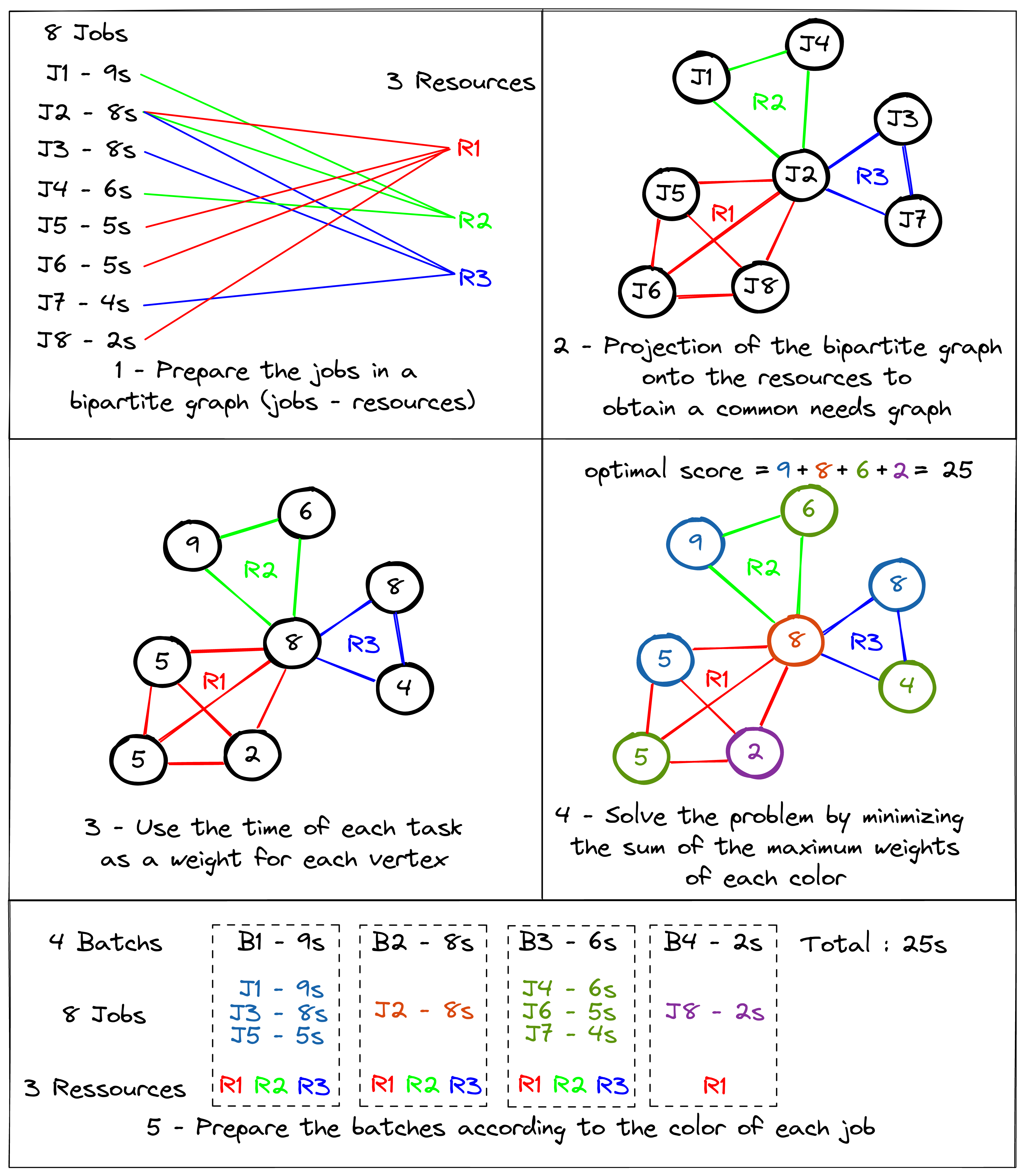
Figure 1: This figure shows an application of the WVCP for scheduling jobs into batches in a multiprocessor environment with restricted access to certain resources.

Different methods have been proposed in the literature to solve the WVCP. First, this problem has been tackled with exact methods: a branch-and-price algorithm furini2012exact and two ILP models proposed in malaguti2009models and Cornaz_Furini_Malaguti_2017 with a transformation of the WVCP into a maximum weight independent set problem. These exact methods can prove the optimality on small instances but fail on large instances.

To handle large graphs, several heuristics have been introduced to solve the problem approximately Nogueira_Tavares_Maciel_2021 ; Prais_Ribeiro_2000 ; Sun_Hao_Lai_Wu_2018 ; Wang_Cai_Pan_Li_Yin_2020 . The first category of heuristics is based on the local search framework, which iteratively makes transitions from the current solution to a neighbor solution. Three different approaches have been considered to explore the search space: legal, partial legal, or penalty strategies. The legal strategy starts from a legal solution and minimizes the score by performing only legal moves so that no color conflict is created in the new solution Prais_Ribeiro_2000 . The partial legal strategy allows only legal coloring and keeps a set of uncolored vertices to avoid conflicts Nogueira_Tavares_Maciel_2021 . The penalty strategy considers both legal and illegal solutions in the search space Sun_Hao_Lai_Wu_2018 ; Wang_Cai_Pan_Li_Yin_2020 , and uses a weighted evaluation function to minimize both the WVCP objective function and the number of conflicts in the illegal solutions. To escape local optima traps, these local search algorithms incorporate different mechanisms such as perturbation strategies Prais_Ribeiro_2000 ; Sun_Hao_Lai_Wu_2018 , tabu list Nogueira_Tavares_Maciel_2021 ; Sun_Hao_Lai_Wu_2018 and constraint reweighting schemes Wang_Cai_Pan_Li_Yin_2020 .

The second category of existing heuristics for the WVCP relies on the population-based memetic framework that combines local search with crossovers. A recent algorithm Goudet_Grelier_Hao_2021 of this category uses a deep neural network to learn an invariant by color permutation regression model, useful to select the most promising crossovers at each generation.

Research on combining such learning techniques and heuristics has received increasing attention in the past years zhou2018improving ; zhou2020frequent . In these new frameworks, useful information (e.g., relevant patterns) is learned from past search trajectories and used to guide a local search algorithm.

This study continues on this path and investigates the potential benefits of combining Monte Carlo Tree Search (MCTS) and sequential coloring or local search algorithms for solving the WVCP. MCTS is a heuristic search algorithm that generated considerable interest due to its spectacular success for the game of Go gelly2006modification , and in other domains (see the survey browne2012survey on this topic). It has been recently revisited in combination with modern deep learning techniques for difficult two-player games (cf. AlphaGo Silver_Huang_Maddison_2016 ). MCTS has also been applied to combinatorial optimization problems seen as a one-player game such as the traveling salesman problem edelkamp2014solving or the knapsack problem Jooken_Leyman_2020 . An algorithm based on MCTS has recently been implemented with some success for the GCP in Cazenave_Negrevergne_Sikora_2020 . In this work, we investigate for the first time the MCTS approach for solving the WVCP.

In MCTS, a tree is built incrementally and asymmetrically. For each iteration, a tree policy balancing exploration and exploitation is used to find the most critical node to expand. A simulation is then run from the expanded node and the search tree is updated with the result of this simulation. Its incremental and asymmetric properties make MCTS a promising candidate for the WVCP because in this problem only the heaviest vertex of each color group has an impact on the objective score. Therefore learning to color the heaviest vertices of the graph before coloring the rest of the graph seems particularly relevant for this problem. The contributions of this work are summarized as follows.

First, we present a MCTS algorithm dedicated to the WVCP, which considers the problem from the perspective of sequential coloring with a predefined vertex order. The exploration of the tree is accelerated with the use of specific pruning rules, which offer the possibility to explore the whole tree in a reasonable amount of time for small instances and to obtain optimality proofs. Secondly, for large instances, when obtaining an exact result is impossible in a reasonable time, we study how this MCTS algorithm can be tightly coupled with other heuristics. Specifically, we investigate the integration of different greedy coloring strategies and local search procedures within the MCTS algorithm.

The rest of the paper is organized as follows. Section 2 introduces the weighted vertex coloring problem and the constructive approach with a tree. Section 3 describes the MCTS algorithm devised to tackle the problem. Section 4 presents the coupling of MCTS with local search. Section 5 reports computational results of different versions of MCTS. Section 6 discusses the contributions and presents research perspectives.

2 Constructive approach with a tree for the weighted graph coloring problem

This section presents a tree-based approach for the WVCP, which aims to explore the partial and legal search space of this problem.

2.1 Partial and legal search space

The search space $\Omega$ studied in our algorithm concerns legal, but potentially partial, $k$-colorings. A partial legal $k$-coloring $S$ is a partition of the set of vertices $V$ into $k$ disjoint independent sets $V_{i}$ ($1\leq i\leq k$), and a set of uncolored vertices $U=V\backslash\bigcup_{i=1}^{k}V_{i}$. A independent set $V_{i}$ is a set of mutually non adjacent vertices of the graph: $\forall u,v\in V_{i},(u,v)\notin E$. For the WVCP, the number of colors $k$ that can be used is not known in advance. Nevertheless, it is not lower than the chromatic number of the graph $\chi(G)$ and not greater than the number of vertices $n$ of the graph. A solution of the WVCP is denoted as partial if $U\neq\emptyset$ and complete otherwise. The objective of the WVCP is to find a complete solution $S$ with a minimum score $f(S)$ given by: $f(S)=\sum_{i=1}^{k}\max_{v\in V_{i}}{w(v)}.$

2.2 Tree search for weighted vertex coloring

Backtracking-based tree search is a popular approach for the graph coloring problem brelaz1979new ; KubaleJ84 ; lewis_guide_2021 . In our case, a tree search algorithm can be used to explore the partial and legal search space of the WVCP previously defined.

Starting from a solution where no vertex is colored (i.e., $U=V$) and that corresponds to the root node $R$ of the tree, child nodes $C$ are successively selected in the tree, consisting of coloring one new vertex at a time. This process is repeated until a terminal node $T$ is reached (all the vertices are colored). A complete solution (i.e., a legal coloring) corresponds thus to a branch from the root node to a terminal node.

The selection of each child node corresponds to applying a move to the current partial solution being constructed. A move consists of assigning a particular color $i$ to an uncolored vertex $u\in U$, denoted as $<u,U,V_{i}>$. Applying a move to the current partial solution $S$, results in a new solution $S\ \oplus<u,U,V_{i}>$. This tree search algorithm only considers legal moves to stay in the partial legal space. For a partial solution $S=\{V_{1},...,V_{k},U\}$, a move $<u,U,V_{i}>$ is said legal if no vertex of $V_{i}$ is adjacent to the vertex $u$. At each level of the tree, there is at least one possible legal move that applies to a vertex a new color that has never been used before (or putting this vertex in a new empty set $V_{i}$, $k+1\leq i\leq n$).

Applying a succession of $n$ legal moves from the initial solution results in a legal coloring of the WVCP and reaches a terminal node of the tree. During this process, at the level $t$ of the tree ($0\leq t<n)$, the current legal and partial solution $S=\{V_{1},...,V_{k},U\}$ has already used $k$ colors and $t$ vertices have already received a color. Therefore |$U$|$=n-t$.

At this level, a first naive approach could be to consider all the possible legal moves, corresponding to choosing a vertex in the set $U$ and assigning to the vertex a color $i$, with $1\leq i\leq n$. This kind of choice can work with small graphs but with large graphs, the number of possible legal moves becomes huge. Indeed, at each level $t$, the number of possible legal moves can go up to $(n-t)\times n$. To reduce the set of move possibilities, we consider the vertices of the graph in a predefined order $(v_{1},\dots,v_{n})$. Moreover, to choose a color for the incoming vertex, we consider only the colors already used in the partial solution plus one color (creation of a new independent set). Thus for a current legal and partial solution $S=\{V_{1},...,V_{k},U\}$, at most $k+1$ moves are considered. The set of legal moves is:

$$\mathcal{L}(S)=\{<u,U,V_{i}>,1\leq i\leq k,\forall v\in V_{i},(u,v)\notin E\}\ \cup<u,U,V_{k+1}>$$ (1)

This decision cuts the symmetries in the tree while reducing the number of branching factors at each level of the tree.

2.3 Predefined vertex order

We propose to consider a predefined ordering of the vertices, sorted by weight and then by degree. Vertices with higher weights are placed first. If two vertices have the same weight, then the vertex with the higher degree is placed first. This order is intuitively relevant for the WVCP because it is more important to place first the vertices with heavy weights which have the most impact on the score as well as the vertices with the highest degree because they are the most constrained decision variables. Such ordering has already been shown to be effective with greedy constructive approaches for the GCP brelaz1979new and the WVCP Nogueira_Tavares_Maciel_2021 .

Moreover, this vertex ordering allows a simple score calculation while building the tree. Indeed, as the vertices are sorted by descending order of their weights, and the score of the WVCP only counts the maximum weight of each color group, with this vertex order, the score only increases by the value $w(v)$ when a new color group is created for the vertex $v$.

3 Monte Carlo Tree Search for weighted vertex coloring

The search tree presented in the last subsection can be huge, in particular for large instances. Therefore, in practice, it is often impossible to perform an exhaustive search of this tree, due to expensive computing time and memory requirements. We turn now to an adaptation of the MCTS algorithm for the WVCP to explore this search tree. MCTS keeps in memory a tree (hereinafter referred to as the MCTS tree) that only corresponds to the already explored nodes of the search tree presented in the last subsection. In the MCTS tree, a leaf is a node whose children have not yet all been explored while a terminal node corresponds to a complete solution. MCTS can guide the search toward the most promising branches of the tree, by balancing exploitation and exploration and continuously learning at each iteration.

3.1 General framework

The MCTS algorithm for the WVCP is shown in Algorithm 1. The algorithm takes a weighted graph as input and tries to find a legal coloring $S$ with the minimum score $f(S)$. The algorithm starts with an initial solution where the first vertex is placed in the first color group. This is the root node of the MCTS tree. Then, the algorithm repeats several iterations until a stopping criterion is met. At every iteration, one legal solution is completely built, which corresponds to walking along a path from the root node to a leaf node of the MCTS tree and performing a simulation (or playout/rollout) until a terminal node of the search tree is reached (when all vertices are colored).

Each iteration of the MCTS algorithm involves the execution of 5 steps to explore the search tree with legal moves (cf. Section 2):

1. Selection From the root node of the MCTS tree, successive child nodes are selected until a leaf node is reached. The selection process balances the exploration-exploitation trade-off. The exploitation score is linked to the average score obtained after having selected this child node and is used to guide the algorithm to a part of the tree where the scores are the lowest (the WVCP is a minimization problem). The exploration score is linked to the number of visits to the child node and will incite the algorithm to explore new parts of the tree, which have not yet been explored.

2. Expansion The MCTS tree grows by adding a new child node to the leaf node reached during the selection phase.

3. Simulation From the newly added node, the current partial solution is completed with legal moves, randomly or by using heuristics.

4. Update After the simulation, the average score and the number of visits of each node on the explored branch are updated.

5. Pruning If a new best score is found, some branches of the MCTS tree may be pruned if it is not possible to improve the best current score with it.

The algorithm continues until one of the following conditions is reached:

• there are no more child nodes to expand, meaning the search tree has been fully explored. In this case, the best score found is proven to be optimal.

• a cutoff time is attained. The minimum score found so far is returned. It corresponds to an upper bound of the score for the given instance.

Algorithm 1 MCTS algorithm for the WVCP

1:Input: Weighted graph $G=(V,W,E)$

2:Output: The best legal coloring $S^{*}$ found

3:$S^{*}=\emptyset$ and $f(S^{*})=MaxInt$

4:while stop condition is not met do

5:     $C\leftarrow R$ $\ignorespaces\triangleright$ Current node corresponding to the root node of the tree

6:     $S$ $\leftarrow$ $\{V_{1},U\}$ with $V_{1}=\{v_{1}\}$ and $U=V\backslash V_{1}$ $\ignorespaces\triangleright$ Current solution initialized with the first vertex in the first color group

7:     /* Selection */ $\ignorespaces\triangleright$ Section 3.2

8:     while $C$ is not a leaf do

9:         $C$ $\leftarrow$ select_best_child(C) with legal move $<u,U,V_{i}>$

10:         $S\leftarrow S\ \oplus<u,U,V_{i}>$

11:     end while

12:     /* Expansion */ $\ignorespaces\triangleright$ Section 3.3

13:     if C has a potential child, not yet open then

14:         $C$ $\leftarrow$ open_first_child_not_open(C) with legal move $<u,U,V_{i}>$

15:         $S\leftarrow S\ \oplus<u,U,V_{i}>$

16:     end if

17:     /* Simulation */ $\ignorespaces\triangleright$ Section 3.4

18:     complete_partial_solution($S$)

19:     /* Update */ $\ignorespaces\triangleright$ Section 3.5

20:     while $C\neq R$ do

21:         update(C,f(S))

22:         $C\leftarrow$ parent(C)

23:     end while

24:     if $f(S)<f(S^{*})$ then

25:         $S^{*}\leftarrow S$

26:         /* Pruning */ $\ignorespaces\triangleright$ Section 3.6

27:         apply pruning rules

28:     end if

29:end while

30:return $S^{*}$

3.2 Selection

The selection starts from the root node of the MCTS tree and selects children nodes until a leaf node is reached. At every level $t$ of the MCTS tree, if the current node $C_{t}$ is corresponds to a partial solution $S=\{V_{1},...,V_{k},U\}$ with $t$ vertices already colored and $k$ colors used, there are $l$ possible legal moves, with $1\leq l\leq k+1$. Therefore, from the node $C_{t}$, $l$ potential children $C^{1}_{t+1},\dots,C^{l}_{t+1}$ can be selected.

If $l>1$, the selection of the most promising child node can be seen as a multi-armed bandit problem Lai_Robbins_1985 with $l$ levers. This problem of choosing the next node can be solved with the UCT algorithm for Monte Carlo tree search by selecting the child with the maximum value of the following expression Jooken_Leyman_2020 :

$$normalized\_score(C^{i}_{t+1})+c\times\sqrt{\frac{2*ln(nb\_visits(C_{t}))}{nb\_visits(C^{i}_{t+1})}},\ \text{for}\ 1\leq i\leq l.$$ (2)

Here, $nb\_visits(C)$ corresponds to the number of times the node $C$ has been chosen to build a solution. $c$ is a real positive coefficient allowing to balance the compromise between exploitation and exploration. It is set by default to the value of one. $normalized\_score(C^{i}_{t+1})$ corresponds to a normalized score of the child node $C^{i}_{t+1}$ ($1\leq i\leq l$) given by:

$$normalized\_score(C^{i}_{t+1})=\frac{rank(C^{i}_{t+1})}{\sum_{i=1}^{l}rank(C^{i}_{t+1})},$$

where $rank(C^{i}_{t+1})$ is defined as the rank between 1 and $l$ of the nodes $C^{i}_{t+1}$ obtained by sorting from bad to good according their average values $avg\_score(C^{i}_{t+1})$ (nodes that seem more promising get a higher score). $avg\_score(C^{i}_{t+1})$ is the mean score on the sub-branch with the node $C^{i}_{t+1}$ selected obtained after all previous simulations.

3.3 Expansion

From the node $C$ of the MCTS tree reached during the selection procedure, one new child of $C$ is open and its corresponding legal move is applied to the current solution. Among the unopened children, the node associated with the lowest color number $i$ is selected. Therefore the child node needing the creation of a new color (and increasing the score) will be selected last.

3.4 Simulation

The simulation takes the current partial and legal solution found after the expansion phase and colors the remaining vertices. In the original MCTS algorithm, the simulation consists in choosing random moves in the set of all legal moves $\mathcal{L}(S)$ defined by equation (1) until the solution is completed. We call this first version MCTS+Random. As shown in the experimental section, this version is not very efficient as the number of colors grows rapidly. Therefore, we propose two other simulation procedures:

• a constrained greedy algorithm that chooses a legal move prioritizing the moves which do not locally increase the score of the current partial solution $S=\{V_{1},...,V_{k},U\}$:

  $$\mathcal{L}^{g}(S)=\{<u,U,V_{i}>,1\leq i\leq k,\forall v\in V_{i},(u,v)\notin E\}$$ (3)

  It only chooses the move $<u,U,V_{k+1}>$, consisting in opening a new color group and increasing the current score by $w(u)$, only if $\mathcal{L}^{g}(S)=\emptyset$. We call this version MCTS+Greedy-Random.

• a greedy deterministic procedure which always chooses a legal move in $\mathcal{L}(S)$ with the first available color $i$. We call this version MCTS+Greedy.

3.5 Update

Once the simulation is over, a complete solution of the WVCP is obtained. If this solution is better than the best recorded solution found so far $S^{*}$ (i.e., $f(S)<f(S^{*})$), $S$ becomes the new global best solution $S^{*}$.

Then, a backpropagation procedure updates each node $C$ of the whole branch of the MCTS tree which has led to this solution:

• the running average score of each node $C$ of the branch is updated with the score $f(S)$:

  $$avg\_score(C)\leftarrow\frac{avg\_score(C)\times nb\_visits(C)+f(S)}{nb\_visits(C)+1}$$ (4)

• the counter of visits $nb\_visits(C)$ of each node of the branch is increased by one.

3.6 Pruning

During an iteration of MCTS, three pruning rules are applied:

1. during expansion: if the score $f(S)$ of the partial solution associated with a node visited during this iteration of MCTS is equal or higher to the current best-found score $f(S^{*})$, then the node is deleted as the score of a partial solution cannot decrease when more vertices are colored.

2. when the best score $f(S^{*})$ is found, the tree is cleaned. A heuristic goes through the whole tree and deletes children and possible children associated with a partial score $f(S)$ equal or superior to the best score $f(S^{*})$.

3. if a node is completely explored, it is deleted and will not be explored in the MCTS tree anymore. A node is said completely explored if it is a leaf node without children, or if all of its children have already been opened once and have all been deleted. Note that this third pruning step is recursive as a node deletion can result in the deletion of its parent if it has no more children, and so on.

These three pruning rules and the fact that the symmetries are cut in the tree by restricting the set of legal moves considered at each step (see Section 2.2) offer the possibility to explore the whole tree in a reasonable amount of time for small instances. This peculiarity of the algorithm makes it possible to obtain an optimality proof for such instances.

3.7 Toy example

Figure 2 displays one iteration of MCTS for the WVCP on a small graph with seven vertices named A–G with different weights between 2 and 9. On each diagram is displayed the current state of the partial coloring solution being constructed (right) and the current state of the search tree (left). In the search tree, each square represents a node and the number on the bottom right of a square is the score of the corresponding partial solution. On top of each square are written the average score and the number of visits of each node. In addition to the root node (vertex A colored in blue), five nodes have already been opened in the search tree (five iterations of MCTS). The sixth iteration of MCTS proceeds as follows.

• Selection: from the root node, the only possible child corresponding to the vertex B in green is selected. From there, there are two options as vertex C can be colored in green or red. The most interesting option is chosen (vertex C in green) regarding the score and the number of visits of each child (cf. equation (2)). Then, the most promising leaf is selected (D in green).

• Expansion: From the node D in green, a new node is added to the tree. It corresponds to E in red (as it cannot take the color blue nor green).

• Simulation: From there, the solution is completed with a greedy algorithm to obtain a complete legal solution with a score of 24.

• Update: this score of 24 is back-propagated on the explored branch (update of the average score and the number of visits of each node in the branch).

• Pruning: Figure 3 presents the state of the tree after some iterations. As the best-found score is 24, every branch of the tree with a score upper or equal to 24 is deleted (indicated with a red cross).

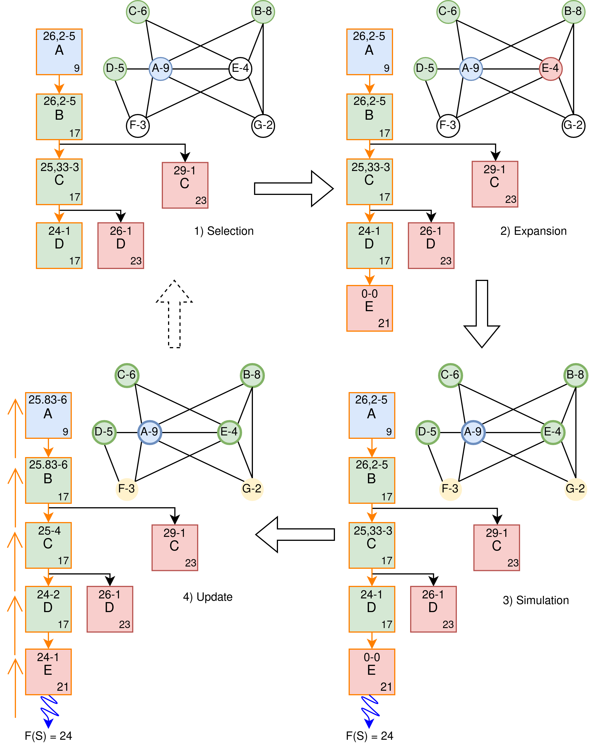
Figure 2: Toy example of one MCTS iteration

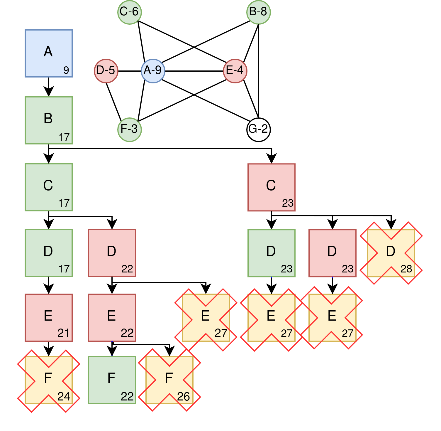
Figure 3: Toy example of the search tree pruning

4 Combining MCTS with Local Search

We now explore the possibility of improving the MCTS algorithm with local search. Coupling MCTS with a local search algorithm is motivated by the fact that after the simulation phase, the complete solution obtained can be close to a still better solution in the search space that could be discovered by local search. In this work, we present the coupling of MCTS with a baseline tabu search (TW) created for this work, as well as three state of the art local search algorithms, dedicated for the WVCP: AFISA Sun_Hao_Lai_Wu_2018 , RedLS Wang_Cai_Pan_Li_Yin_2020 and ILSTS Nogueira_Tavares_Maciel_2021 .

During the simulation phase, the solution is first completed with a greedy algorithm and then improved by the local search procedure. Note that in the first version of this work published in GrelierGH22 , to stay consistent with the search tree learned by MCTS, we allowed the local search procedure to only move the vertices of the complete solution $S$ which are still uncolored after the selection and expansion phases. However, we have realized in the meantime that blocking vertices for the local search can lead to a lot of time spent checking for blocked vertices in the complex neighborhood explored by the various local search procedures. It also leads to missing good opportunities to move in the search space. Therefore, in the new version of the algorithm presented in this paper, a more efficient version of the algorithm is presented where the vertices are not frozen during the local search. In this new version, when coupling MCTS with a local search algorithm, the resulting heuristic can be seen as an algorithm that attempts to learn a good starting point for the local search procedure, by selecting different best promising backbones of partial solutions in every iteration during the selection phase.

As one iteration does not have the same meaning for each local search, we use a time limit of $t=0.02\times n$ seconds to perform the search, depending on the number of vertices $n$ in the given instance. Once the local search procedure has reached the time limit, the score corresponding to the best legal solution obtained by the local search procedure is used to update all the nodes of the branch which has led to the simulation initiation. In the following subsections, the four different local search procedures used in this work are presented.

4.1 Basic tabu search

The first local search algorithm tested is a simple tabu search, named TabuWeight (TW), inspired by the classical TabuCol algorithm for the GCP Hertz_Werra_1987 . Starting from a legal solution, TW improves it iteratively by using a one move operator, which consists in moving a vertex from its color group to another color group, without creating conflicts. At each iteration, the best one move which is not forbidden by the tabu list is selected. Each time a move is performed, the reverse move is added to the tabu list and forbidden for the next $tt$ iterations where $tt$ is a parameter called tabu tenure. A tabu move can still be applied exceptionally if it leads to a solution, which is better than the best solution found so far (aspiration criterion).

4.2 Adaptive feasible and infeasible tabu search

AFISA Sun_Hao_Lai_Wu_2018 is a tabu search algorithm, which explores the candidate solutions by oscillating between illegal and legal search spaces. To prevent the search from going too far from legal boundaries, AFISA uses a controlling coefficient to adaptively makes the algorithm go back and forth between illegal and legal spaces. The controlling coefficient encourages the algorithm to handle in priority the vertices in conflicts before trying to reduce the WVCP score. AFISA uses the popular one move operator to explore the search space.

4.3 Local search with multiple operators

Like AFISA, RedLS Wang_Cai_Pan_Li_Yin_2020 explores the illegal and legal search spaces. This algorithm uses the configuration checking strategy cai_local_2011 that applies multiple improvements and perturbation strategies to explore the search space. At each iteration, RedLS perturbs the solution by moving all the heaviest vertices from one color group to another group, before minimizing the number of conflicts to recover a new legal solution. It uses different variants of the one move operator to reduce the number of conflicts while keeping the WVCP score as low as possible. Each conflicting edge has a weight that is increased each time it is not resolved, to give priority to its resolution for the next iterations.

4.4 Iterated local search with tabu search

ILSTS Nogueira_Tavares_Maciel_2021 explores the legal and partial search spaces. From a complete solution, the ILSTS algorithm iteratively performs 2 steps: (i) it deletes the heaviest vertices from 1 to 3 color groups $V_{i}$ and places them in the set of uncolored vertices $U$; (ii) it improves the solution (i.e., minimizes the score $f(S)$) by applying different variants of the one move operator and the so-called grenade operator until the set of uncolored vertices $U$ becomes empty. The grenade operator $grenade(u,V_{i})$ consists in moving a vertex $u$ to $V_{i}$, but first, each adjacent vertices of $u$ in $V_{i}$ is relocated to other color groups or in $U$ to keep a legal solution.

5 Experimentation

This section first describes the experimental settings used in this work. Secondly, we experimentally verify the impacts of the different greedy coloring strategies used during the MCTS simulation phase. Thirdly, an analysis of exploration versus exploration is performed. Lastly, the relevance of coupling MCTS with a local search procedure is studied.

5.1 Experimental settings and benchmark instances

A total of 188 instances are used for the experimental studies: 30 rxx graphs and 35 pxx graphs from matrix decomposition Prais_Ribeiro_2000 and 123 from the DIMACS and COLOR competitions. Two pre-processing procedures were applied to reduce the graphs of the different instances. The first one comes from Wang_Cai_Pan_Li_Yin_2020 : if the weight of a vertex of degree $d$ is lower than the weight of the $d+1$th heaviest vertex from any clique of the graph, then the vertex can be deleted without changing the optimal WVCP score of this instance. The second one comes from Cheeseman_Kanefsky_Taylor_1991 and is adapted to our problem: if all neighbors of a vertex $v1$ are all neighbors with a vertex $v2$ and the weight of $v2$ is greater or equal to the weight of $v1$, then $v1$ can be deleted as it can take the color of $v2$ without impacting the score. All the original and reduced instances are available at https://github.com/Cyril-Grelier/gc_instances.

All presented algorithms are coded in C++, compiled, and optimized with the g++ 12.1 compiler. The source code of our algorithm (and reproduced local searches) is available at https://github.com/Cyril-Grelier/gc_wvcp_mcts with complete spreadsheets of the results. To solve each instance, 20 independent runs were performed on a computer equipped with an Intel Xeon ES 2630, 2,66 GHz CPU with a time limit of one hour, except for the exploration vs. exploitation coefficient tests where 5 to 15 hours were used. Running the DIMACS Machine Benchmark procedure dfmax on our computer took 8.94 seconds to solve the instance r500.5 using gcc 12.1 without optimization flag.

In the following subsections, summary tables allowing general comparisons between the different versions of the algorithms are presented. Detailed results on each specific instance are reported in appendices A.1 and A.2.

The 188 instances have been separated into four sets: (i) pxx, with the 35 pxx instances from Prais_Ribeiro_2000 , (ii) rxx, with the 30 rxx instances from Prais_Ribeiro_2000 , (iii) DIMACS_easy, corresponding to the easy 59 DIMACS and COLOL instances which were solved optimally by the exact algorithm MWSS Cornaz_Furini_Malaguti_2017 or the MCTS greedy variants, reported in Nogueira_Tavares_Maciel_2021 (launched with a time limit of 10 hours for each instance), and (iv) DIMACS_hard, the 64 hard DIMACS instances which have never been solved optimally in the literature.

For all the different versions of the MCTS algorithm, the coefficient $c$, allowing to balance the compromise between exploitation and exploration is set to the value of one (cf. equation (2)). A sensitivity analysis of this important hyperparameter is conducted in Section 5.3.

5.2 Monte Carlo Tree Search with greedy strategies

Table 1 summaries the results of MCTS with greedy heuristics for its simulation (cf. Section 3.4). Columns 1 and 2 show the instance sets and their size (a star is added if all the instances of the set have optimally been solved). Columns 3-8 show the number of instances for which each method can achieve the Best Known Score (BKS) from the literature. Some of the BKS come from Nogueira_Tavares_Maciel_2021 (1h runs) or Goudet_Grelier_Hao_2021 (many hours of calculation), otherwise, they come from our reproductions of the state of the art algorithms. The numbers indicated with a star and in parenthesis in this table correspond to the number of times the method can prove that the best score obtained is optimal.

Column 3 shows the results of a random algorithm (R) which colors each vertex one by one with a random color. Column 4 presents the results of the MCTS+Random algorithm with the random simulation (MCTS+R). Column 5 reports the results of the greedy random procedure alone (GR). This GR procedure colors each vertex one by one with a random already used color and opens a new color when it is mandatory. Column 6 reports the results of the MCTS algorithm using this simulation strategy (MCTS+GR). Column 7 corresponds to the deterministic greedy strategy (G). This strategy consists in always choosing the first available color for each vertex and opening new colors only if needed. Column 8 shows the results of MCTS+Greedy coupling MCTS with this deterministic greedy strategy (MCTS+G).

Table 1: Summary of the number of times the Best Known Score is reached for each algorithm. The values with a star indicate the number of times a score has been proved optimal. Values in bold highlight the best results for each line.

instances	|I|	R	MCTS+R	GR	MCTS+GR	G	MCTS+G
pxx	35*	1	34 (25*)	13	35 (25*)	13	35 (25*)
rxx	30*	0	1	0	20	2	11
DIMACS_easy	59*	3	32 (19*)	11	45 (20*)	8	35 (19*)
DIMACS_hard	64	0	7	2	8	1	6
Total	188	4	74 (44*)	26	108 (45*)	24	87 (44*)

First, we observe that all the MCTS variants dominate the baseline greedy algorithms (R, G, and GR) in terms of the number of the BKS obtained, highlighting the relevance of combining the MCTS framework and search heuristics.

With the coupled MCTS algorithms, almost all pxx instances are solved. The rxx instances are more difficult to solve except for the version MCTS+Greedy-Random. The instances from DIMACS_easy are partially solved by each MCTS variant. The instances from DIMACS_hard show a real difficulty for all these MCTS variants, because very few methods reach the BKS of the literature.

To better compare these different algorithms, and not only relying on the number of best-known scores achieved (that can sometimes be found by ”chance”), we performed pairwise comparisons between the algorithms based on the average scores obtained on each instance as displayed in Table 2.

In Table 2, the numbers in each row correspond to the number of instances for which the method is significantly better than another (with a maximum of 188 instances). A method is said significantly better than another on a given instance if its average score measured over 20 runs is significantly better (t-test with a p-value below 0.001). The column Total corresponds to the number of times a method is better than another.

Table 2: Comparison between all greedy and MCTS variants. As an example, the row for MCTS+Random means that the method is better on 188 instances compared to the random procedure (R), on 165 instances compared to the Greedy-Random procedure (GR), and never compared to MCTS+Greedy-Random (MCTS+GR). Values in bold highlight the highest value between two methods, the variant MCTS+Greedy is more often (49 times) significantly better than MCTS+Greedy-Random (which is better than MCTS+Greedy 25 times).

	R	MCTS+R	GR	MCTS+GR	G	MCTS+G	Total
R	-	0	0	0	0	0	0/5
MCTS+R	188	-	165	0	95	1	3/5
GR	188	11	-	0	6	0	1/5
MCTS+GR	188	125	179	-	152	25	4/5
G	188	41	150	10	-	0	2/5
MCTS+G	188	122	179	49	160	-	5/5

Table 2 highlights the ranking of each method. Unsurprisingly, the pure random heuristic is completely dominated by all methods. The variant MCTS+Greedy is significantly better compared to the others. In particular, it stays significantly better 49 times out of 188, versus 25 times in favor of the MCTS+Greedy-Random. Indeed, it seems that for the WVCP, the greedy procedure, forcing the heaviest vertices to be grouped in the first colors enables a better organization of the color groups. This is particularly true for the largest instances, where choosing random moves in the set of all legal moves is not very efficient as the number of color groups grows rapidly. It explains also why the variant MCTS+Random performs badly on larger or denser instances such as the rxx instances or some difficult DIMACS instances.

However, with the deterministic simulation of the MCTS+Greedy variant, there is no sampling of the legal moves like in the MCTS+Greedy-Random variant allowing greater exploration of the search space and a better estimation of the most promising branches of the search tree. This particularity of the MCTS+Greedy-Random variant allows us to find the BKS for more instances (see Table 1). Moreover, when exploring the results in the Appendix A.1, one can see that the R75_1gb instance from the DIMACS_easy set is proved optimal by MCTS+Greedy-Random but not by MCTS+Greedy. With stochastic help, the MCTS+Greedy-Random version can reach the best know score of 70, which leads to an early pruning of the tree that allows proving the optimality earlier.

5.3 Exploitation vs exploration coefficient analysis

One key element of the MCTS algorithm is the coefficient $c$ balancing the compromise between exploration and exploitation in equation (2). In this subsection, we investigate the importance of this coefficient by varying it and presenting the evolution of the score over time. For this experimentation, we varied the coefficient $c$ from 0 (no exploration) to 5 (encourage exploration). For each coefficient value, we performed 20 runs of the MCTS+Greedy-Random variant per instance during 5h per run (15h for the very large C2000.x instances).

Figure 4 displays 6 plots showing the evolution of the mean of the best scores over time for the instances DSJC500.5, latin_square_10, le450_25a, wap01a, C2000.5 and C2000.9 for the different values of the coefficient $c$. These 6 instances come from the set of DIMACS_hard instances and can be considered as very difficult.

Four typical patterns also seen for other instances are observed:

• P1: instances requiring a lot of exploration,

• P2: instances requiring more exploration than exploitation,

• P3: instances requiring more exploitation than exploration,

• P4: instances requiring a lot of exploitation.

The first pattern P1 is observed for the instance DSJC500.5 and also queen instances. For these instances, the lack of exploration leads to poor results, and better results are reached as the coefficient $c$ increases. The pattern P2 is observed for the instance latin_square_10, but also for other instances such as flat1000 where the best score obtained in function of the coefficient $c$ has a U-shape, with an optimal value of $c$ between 1 and 2. This phenomenon can also be observed on instances such as C2000.5 and C2000.9 where it becomes quickly more interesting to explore up to a certain point. The pattern P3 found for the le450 instance shows the best results when there is only weak exploration, but the results are worse when $c$ is set to zero.

In general, for the patterns P1, P2 and P3, having no exploration at all rapidly leads to a local minimum trap and it seems better to secure a minimum of diversity to reach a better score, while, for the pattern P4, found for the wap instances (very large instances), giving a chance to the exploration leads the algorithm to be lost in the search space. For very large instances, as the search tree is huge and cannot be sufficiently explored due to the time limit, it seems more beneficial for the algorithm to favor more intensification to better search for a good solution in a small part of the tree. To sum, the most suitable exploration vs exploitation coefficient thus depends on the instance considered. Finding the right general coefficient is a challenging task. In this work, We adopted the coefficient $c=1$ for all other experiments.

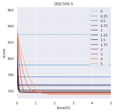
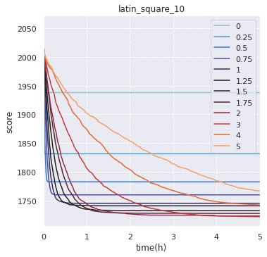
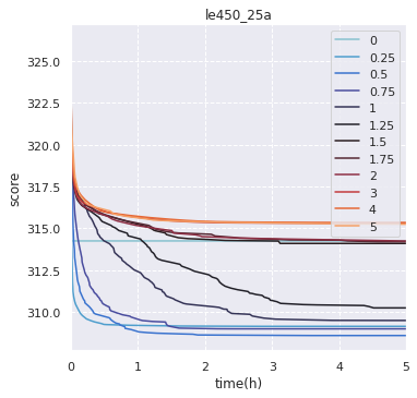
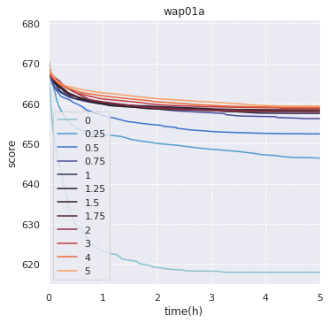
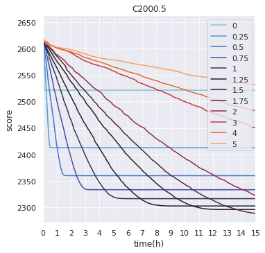
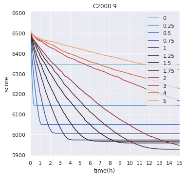
Figure 4: Plots of the evolution of the means of the scores over time for different values of the coefficient $c$ between 0 and 5, for the instances DSJC500.5, latin_square_10, le450_25a, wap01a, C2000.5, and C2000.9. For each configuration, 20 runs are launched with the MCTS+Greedy-Random variant for 5h and 15h for the C2000 instances.

5.4 Monte Carlo Tree Search with local search

This section studies the effects of the combination of MCTS with a local search heuristic. Table 3 summarizes the results of the local search procedures presented in Section 4 followed by the combination of MCTS with each of these local search procedures during the simulation phase. Each line presents the number of times a BKS is reached with the method. Note that the objective of these MCTS variants coupled with a local search procedure is not to prove optimality. For instances where the optimal score is known, MCTS and local search stop when this score is reached.

Table 3: Summary of the number of times the Best Known Score is reached for the local search procedures and MCTS combined with the different local search procedures. Values in bold highlight the best results for each line.

instances	|I|	AFISA	MCTS+AFISA	TW	MCTS+TW	RedLS	MCTS+RedLS	ILSTS	MCTS+ILSTS
pxx	35*	34	34	26	34	29	35	35	35
rxx	30*	5	6	7	17	7	26	30	30
DIMACS_easy	59*	55	58	42	54	54	58	58	58
DIMACS_hard	64	18	22	20	23	28	34	27	27
Total	188	112	120	95	128	118	153	150	150

We observe from this table that the local search procedure allowing to reach the highest number of BKS is ILTS, followed by RedLS. TW, AFISA, and RedLS also improve their results when coupled with the MCTS framework. In particular, the variant MCTS+RedlLS finds the BKS for 34 difficult instances of the DIMACS_hard set and 153 instances over 188 in total, which is better than all other algorithms tested in this study. Moreover, it is worth noting that this combination allowed to find two new records for the difficult DIMACS instances le450_15a and queen12_12gb that were never reported in the literature (see detailed results in Tables 15 and 16). It highlights that the MCTS framework proposed in this paper can help a local search algorithm such as RedLS to continuously find new promising starting points in the search space.

However, when coupled with the ILSTS algorithm (variant MCTS+ILTS), it does not seem to improve the results. It may be explained by the fact that ILSTS is an iterated local search algorithm already integrating various perturbation mechanisms allowing to escape local optima. Therefore, finding new good starting points in the search space guided by MCTS seems less interesting for ILSTS than for other local search procedures such as TW, AFISA, and RedLS.

Table 4 shows pairwise comparisons between all the MCTS variants and all the local search procedures.

Table 4: Comparison between all the MCTS (MC) variants and all the local search procedures. Each row corresponds to the number of times the method of the row is significantly better than the method on the column on the 188 instances. NOT CLEAR, REPHRASE For example, out of 188 instances, TW is better than MCTS+TW on 24 instances, 43 times against RedLS and 5 times against MCTS+RedLS. Values in bold means that method $a$ is more often better than method $b$ when we look at how many time $b$ is significantly better than $a$. The Total column corresponds to the number of times a method is in bold on the line.

	MCTS+GR	MCTS+G	AFISA	MCTS+AFISA	TW	MCTS+TW	RedLS	MCTS+RedLS	ILSTS	MCTS+ILSTS	Total
MCTS+GR	-	25	43	30	50	15	55	2	7	12	0/9
MCTS+G	49	-	54	48	60	28	56	10	16	24	4/9
AFISA	45	35	-	22	33	14	34	1	12	18	1/9
MCTS+AFISA	56	47	62	-	62	6	66	3	1	8	4/9
TW	60	55	56	40	-	24	43	5	18	27	2/9
MCTS+TW	74	62	76	64	73	-	76	7	13	25	6/9
RedLS	62	68	62	43	61	38	-	15	28	33	4/9
MCTS+RedLS	95	94	103	73	104	65	97	-	39	43	9/9
ILSTS	90	79	88	71	83	45	81	13	-	37	8/9
MCTS+ILSTS	84	77	80	62	74	36	80	13	0	-	7/9

When comparing the performances of the local search algorithms by looking at the number of times they are significantly better than the others in terms of average score, AFISA and TW switch their ranks, and RedLS and ILSTS keep the second and first place.

When comparing MCTS+Greedy-Random and MCTS+Greedy to the local search or MCTS+local_search variants, MCTS+Greedy-Random does not show much success compared to MCTS+Greedy, which has better results more often against AFISA, MCTS+AFISA, and TW for a few more instances.

The MCTS+local_search variants always improve the number of BKS found and are more often significantly better than the corresponding local search only, except for ILSTS, which is better on its own and dominates the MCTS+ILSTS variant.

The variant MCTS+RedLS is significantly better than the other methods, even compared to ILSTS only. These results indicate that combining MCTS with a local search is of interest to improve the underlying local search procedures such as AFISA, TW, and RedLS.

6 Conclusions

In this work, we investigated Monte Carlo Tree Search applied to the weighted vertex coloring problem. We studied different greedy strategies and local searches used for the simulation phase. Our experimental results lead to three conclusions.

When the instance is large and when a time limit is imposed, MCTS does not have the time to learn promising areas in the search space and it seems more beneficial to favor more intensification, which can be done in three different ways: (i) by lowering the coefficient which balances the compromise between exploitation and exploration during the selection phase, (ii) by using a dedicated heuristic exploiting the specificity of the problem (grouping in priority the heaviest vertices in the first groups of colors), (iii) and by using a local search procedure to improve the complete solution.

Conversely, for small instances, it seems more beneficial to encourage more exploration, to avoid getting stuck in local optima. It can be done, by increasing the coefficient, which balances the compromise between exploitation and exploration, and by using a simulation strategy with more randomness, which favors more exploration of the search tree and also allows a better evaluation of the most promising branches of the MCTS tree. For these small instances, the MCTS algorithm can provide some optimality proofs.

For medium instances, it seems important to find a good compromise between exploration and exploitation. For such instances, coupling the MCTS algorithm with a local search procedure allows finding better solutions, which cannot be reached by the MCTS algorithm or the local search alone.

Other future works could be envisaged. For example, an interesting study would be to automatically choose the balance coefficient between exploitation and exploration on the fly when solving each specific instance. It could also be interesting to use a more adaptive approach to trigger the local search, or to use a machine-learning algorithm to guide the search toward more promising branches of the search tree.

Authors’ contributions

C. Grelier developed the code, prepared the reduced instances, and performed the tests. O. Goudet and J.K. Hao planned and supervised the work. All the authors contributed to the analysis and the writing of the manuscript.

Conflict of Interest

The authors declare that they have no conflicts of interest.

Availability of data set, code, and results

The instances used in this work are available at https://github.com/Cyril-Grelier/gc_instances. The codes of the tested methods and their detailed results are available at https://github.com/Cyril-Grelier/gc_wvcp_mcts.

Appendix A Appendix

In this Appendix, we present the detailed results on each instance of the different algorithms presented in this paper. In each of the following tables, the first column is the instance name followed by the number of vertices, the number of edges, and the best-known scores of the literature. Then for each method, are displayed the best score, the average score (out of 20 runs), and the average execution time in seconds required to reach the best score.

Best-known scores that are proved optimal are indicated with a star (*) next to the score. Scores in bold means that the score is equal to the BKS, except two times in Tables 15 and 16 when the proposed variant MCTS+RedLS improves the BKS on le450_15a and queen12_12gb (which are indicated with a plus (+)). More readable spreadsheets of those tables (with some more information) can be found in the GitHub repository https://github.com/Cyril-Grelier/gc_instances (follow the indications in the README file).

A.1 Detailed results of MCTS coupled with greedy strategies

Tables 5- 10 report the detailed results for the MCTS variants combined with the greedy strategies (cf. Section 5.2).

Table 5: Results on pxx instances for Greedy and MCTS+Greedy methods.

90 instance |$V$| |$E$| BKS Random MCTS+Random Greedy-Random MCTS+Greedy-Random Greedy MCTS+Greedy best avg time best avg time best avg time best avg time best avg time best avg time p06 16 38 565* 605 853.9 0 565* 565.2 0 565 579 0 565* 565 0 585 585 0 565* 565 0 p07 24 92 3771* 4227 4943.7 0 3771* 3771 0 3846 3951.6 0 3771* 3771 0 3849 3849 0 3771* 3771 0 p08 24 92 4049* 4780 5607.1 0 4049* 4056.5 0 4239 4349.1 0 4049* 4049 0 4294 4294 0 4049* 4049 0 p09 25 100 3388* 3945 5330 0 3388* 3388 0 3443 3557.2 0 3388* 3388 0 3496 3496 0 3388* 3388 0 p10 16 32 3983* 4055 4956.9 0 3983* 3983 0 3983 3986.9 0 3983* 3983 0 3983 3983 0 3983* 3983 0 p11 18 48 3380* 3460 4192.5 0 3380* 3380 0 3380 3389 0 3380* 3380 0 3380 3380 0 3380* 3380 0 p12 26 90 657* 796 1143.2 0 657* 658.5 0 657 758.5 0 657* 657 0 657 657 0 657* 657 0 p13 34 160 3220* 3691 4699.7 0 3220* 3220 0 3230 3387.6 0 3220* 3220 0 3255 3255 0 3220* 3220 0 p14 31 110 3157* 3829 4906.1 0 3157* 3157 0 3157 3403.7 0 3157* 3157 0 3172 3172 0 3157* 3157 0 p15 34 136 341* 441 548 0 341* 341 0 376 380.9 0 341* 341 0 383 383 0 341* 341 0 p16 34 134 2343* 2848 3639.3 0 2343* 2343 0 2348 2478.8 0 2343* 2343 0 2416 2416 0 2343* 2343 0 p17 37 161 3281* 3931 5227.9 0 3281* 3281 0 3281 3584.7 0 3281* 3281 0 3642 3642 0 3281* 3281 0 p18 35 143 3228* 3982 5021.9 0 3228* 3228 0 3339 3524 0 3228* 3228 0 3348 3348 0 3228* 3228 0 p19 36 156 3710* 3960 4668 0 3710* 3710 0 3710 3727.5 0 3710* 3710 0 3710 3710 0 3710* 3710 0 p20 37 142 1830* 2290 3004 0 1830* 1830 0 1910 1962.5 0 1830* 1830 0 1930 1930 0 1830* 1830 0 p21 38 155 3660* 4400 5325 0 3660* 3660 0.7 3830 3923 0 3660* 3660 0 3830 3830 0 3660* 3660 0 p22 38 154 1912* 2237 2831.9 0 1912* 1912 6.5 1935 2003.5 0 1912* 1912 0 1935 1935 0 1912* 1912 0 p23 44 204 3770* 4880 5852.5 0 3770* 3770 4 3940 4043.5 0 3770* 3770 0 3960 3960 0 3770* 3770 1 p24 34 104 661* 819 998.4 0 661* 661 2.2 676 705.8 0 661* 661 0 661 661 0 661* 661 0.3 p25 36 120 504* 620 765.7 0 504* 504 0.8 504 552 0 504* 504 0 504 504 0 504* 504 0 p26 37 131 520* 592 811.2 0 520* 520 0.1 520 535.3 0 520* 520 0 520 520 0 520* 520 0 p27 44 174 216* 302 356.8 0 216 216 0 218 233.9 0 216 216 0 259 259 0 216 216 0 p28 44 164 1729* 2239 2836.8 0 1729* 1729 301.6 1749 1821.9 0 1729* 1729 0 1729 1729 0 1729* 1729 0 p29 53 254 3470* 3470 3830 0 3470* 3470 0 3470 3470 0 3470* 3470 0 3470 3470 0 3470* 3470 0 p30 60 317 4891* 5353 6337 0 4891* 4891 2.8 4902 4918.7 0 4891* 4891 0 4929 4929 0 4891* 4891 0 p31 47 179 620* 625 694.5 0 620* 620 0 620 620 0 620* 620 0 620 620 0 620* 620 0 p32 51 221 2480* 3030 3736.8 0 2480 2483.5 113.2 2480 2505 0 2480 2480 0 2480 2480 0 2480 2480 0 p33 56 258 3018* 3932 4559.4 0 3018 3030.5 44.4 3118 3210.6 0 3018 3018 0 3018 3018 0 3018 3018 0 p34 74 421 1980* 2410 2989 0 1980 1987.5 1 1990 2027.5 0 1980 1980 0 1990 1990 0 1980 1980 0 p35 86 566 2140* 2740 3146 0 2140 2148 4.6 2180 2248 0 2140 2140 0 2170 2170 0 2140 2140 0.1 p36 101 798 7210* 7940 8868.2 0 7210 7210 16.9 7210 7254.2 0 7210 7210 0 7210 7210 0 7210 7210 0.2 p38 87 537 2130* 2820 3239.4 0 2130 2143.5 601.6 2180 2224 0 2130 2130 0 2170 2170 0 2130 2130 0 p40 86 497 4984* 6172 7489.4 0 4984 4991.7 49.9 4998 5093.4 0 4984 4984 0 5020 5020 0 4984 4984 0 p41 116 900 2688* 3377 3993.8 0 2688 2709.6 198.2 2711 2798.1 0 2688 2688 0 2724 2724 0 2688 2688 0 p42 138 1186 2466* 3567 4195.8 0 2489 2514.1 16 2484 2546 0 2466 2466.4 56.5 2517 2517 0 2466 2466 0 nb total best 1/35 34/35 13/35 35/35 13/35 35/35 nb total optim 0/35 25/35 0/35 25/35 0/35 25/35

Table 6: Results on rxx instances for Greedy and MCTS+Greedy methods.

90 instance |$V$| |$E$| BKS Random MCTS+Random Greedy-Random MCTS+Greedy-Random Greedy MCTS+Greedy best avg time best avg time best avg time best avg time best avg time best avg time r01 144 1280 6724* 9956 11532.3 0 6745 6810.6 11 7023 7203.9 0 6724 6725.4 30.8 7138 7138 0 6724 6724 0 r02 142 1246 6771* 10237 11756.8 0 6814 6875.1 10 6849 7232.2 0 6771 6773.6 239.2 6786 6786 0 6771 6771 0 r03 139 1188 6473* 9655 11343.8 0 6531 6642.1 150 6587 6927.9 0 6473 6486.7 0.5 6627 6627 0 6481 6481 2 r04 151 1406 6342* 9611 11182.1 0 6417 6509.6 339 6466 6885.6 0 6342 6356.8 2 6388 6388 0 6342 6342 0 r05 142 1266 6408* 10120 11205.8 0 6443 6626.9 14 6809 6971.9 0 6408 6422.7 368.5 6530 6530 0 6408 6408 0 r06 148 1381 7550* 10215 11976 0 7550 7566.1 62 7557 7787.8 0 7550 7551.3 0.2 7550 7550 0 7550 7550 0 r07 141 1253 6889* 9551 11062.4 0 6911 6977.9 19 6957 7185.6 0 6889 6891.6 63.9 7201 7201 0 6903 6903 0 r08 138 1191 6057* 9138 10507.2 0 6101 6178.4 31 6163 6523.4 0 6057 6062.5 10.1 6146 6146 0 6057 6057 0 r09 129 1027 6358* 9809 11100.7 0 6443 6536.2 8 6564 6685.1 0 6365 6371.5 67 6542 6542 0 6361 6361 31.9 r10 150 1409 6508* 9838 11368 0 6537 6619.9 16 6720 7168.9 0 6509 6522.6 28 6783 6783 0 6525 6525 0.4 r11 208 2247 7654* 12644 14167 0 7764 8006.9 608 8063 8365.5 0 7657 7670.9 444 8080 8080 0 7667 7667 18.6 r12 199 2055 7690* 12280 13929.9 0 7710 7923.8 66 7966 8360.9 0 7695 7701.9 100 7930 7930 0 7697 7697 0 r13 217 2449 7500* 12739 13840.3 0 7554 7788.5 1305 7797 8183.6 0 7501 7513.6 472 7780 7780 0 7534 7534 0.1 r14 214 2387 8254* 12515 14525 0 8267 8381.8 1727 8581 8742.2 0 8254 8254.4 122.7 8270 8270 0 8254 8254 0 r15 198 2055 8021* 11629 13281.5 0 8034 8070.9 103 8031 8113 0 8021 8022.6 0.1 8021 8021 0 8021 8021 0 r16 188 1861 7755* 11760 13072.4 0 7767 7800 43 7780 7884.2 0 7755 7756.5 7.6 7764 7764 0 7755 7755 0 r17 213 2392 7979* 12648 14227 0 8219 8316.5 1438 8514 8682.8 0 7979 7986.8 270 8214 8214 0 8033 8033 0 r18 200 2079 7232* 11639 13488.4 0 7257 7569.4 865 7623 7865.1 0 7232 7244.1 39.3 7716 7716 0 7264 7264 48.6 r19 185 1803 6826* 10732 12774.1 0 6910 7161.6 37 7221 7636.8 0 6826 6832.4 20.7 7296 7296 0 6884 6884 3.1 r20 217 2447 8023* 12571 14407.2 0 8072 8157.1 58 8252 8539.6 0 8023 8029.8 27.4 8061 8061 0 8040 8040 4 r21 281 3554 9284* 14720 16733.1 0 9340 9556.1 312 9604 9836.1 0 9286 9293.4 38 9495 9495 0 9288 9288 915.1 r22 285 3684 8887* 14321 16357.1 0 8953 9026 129 9138 9461.8 0 8889 8897 464 9014 9014 0 8890 8890 0.2 r23 288 3732 9136* 14778 16697.1 0 9213 9318 185 9376 9727.9 0 9138 9143.8 293.7 9239 9239 0 9143 9143 28.1 r24 269 3284 8464* 13941 15415.5 0 8540 8638.3 196 8615 9026.4 0 8464 8469.5 53 8484 8484 0 8464 8464 0 r25 266 3177 8426* 13328 15781.5 0 8560 8707.9 94 8862 9035.8 0 8443 8460.4 289 8583 8583 0 8448 8450.5 2690.2 r26 284 3629 8819* 14503 16446.4 0 8929 9037.7 136 8998 9334 0 8826 8847.1 70 9013 9013 0 8826 8826 0.6 r27 259 3019 7975* 13031 15207.5 0 8005 8198.6 936 8320 8663.4 0 7975 7979.4 100 8003 8003 0 7980 7980 1 r28 288 3765 9407* 14948 16739.8 0 9452 9566.5 262 9642 9879.3 0 9407 9409.5 1512.2 9409 9409 0 9407 9407 0 r29 281 3553 8693* 14419 16174.4 0 8821 9030.6 182 9105 9342.7 0 8693 8696.8 1934.8 8973 8973 0 8694 8694 0 r30 301 4122 9816* 14526 16941.2 0 9826 9887.5 374 10057 10227.5 0 9816 9819.9 6 9831 9831 0 9818 9818 0.1 nb total best 0/30 1/30 0/30 20/30 2/30 11/30 nb total optim 0/30 0/30 0/30 0/30 0/30 0/30

Table 7: Results on DIMACS instances with proven optima for Greedy and MCTS+Greedy methods (1/2).

90 instance |$V$| |$E$| BKS Random MCTS+Random Greedy-Random MCTS+Greedy-Random Greedy MCTS+Greedy best avg time best avg time best avg time best avg time best avg time best avg time DSJC125.9g 125 6961 169* 207 217.8 0 172 176.6 2040 180 186.4 0 171 172.7 2045.3 182 182 0 173 173 1 DSJC125.9gb 125 6961 604* 732 765.6 0 614 631.9 1640 647 669.1 0 614 617.5 377.5 656 656 0 621 621 1 DSJC250.9 250 27897 934* 1231 1265.5 0 1009 1029.2 16 1059 1092.2 0 975 987.4 47 1078 1078 0 982 982 12.1 GEOM100 97 530 65* 104 119.4 0 66 67.8 1380.5 68 72.8 0 65 65.3 22.8 71 71 0 65 65 50.6 GEOM100a 97 957 89* 125 135 0 91 94.3 23 96 102.3 0 89 90 22 101 101 0 91 91 1.2 GEOM100b 97 1030 32* 45 50.1 0 32 34.5 1781 35 37.4 0 32 32 0.1 36 36 0 32 32 1 GEOM110 107 619 68* 110 129.5 0 70 73.1 4 73 75.8 0 68 68 23.8 73 73 0 69 69 83.5 GEOM110a 108 1182 97* 136 149.6 0 102 105.3 3088 108 111.5 0 98 100 3 110 110 0 100 100 732.9 GEOM110b 107 1234 37* 47 54.5 0 38 38.1 59.2 39 40.5 0 37 37.4 107.5 40 40 0 38 38 0 GEOM120 117 754 72* 111 127.2 0 75 76.9 4 77 81.7 0 72 72.5 17.1 80 80 0 72 72 0 GEOM120a 118 1406 105* 150 159.2 0 109 111.5 46.3 118 121.8 0 106 106.6 78.6 120 120 0 105 105 1365.9 GEOM120b 118 1477 35* 52 57 0 38 38.5 16.2 40 41.7 0 36 37 0 40 40 0 37 37.5 3543.3 GEOM20 17 19 33* 33 37.5 0 33* 33 0 33 33 0 33* 33 0 33 33 0 33* 33 0 GEOM20a 12 19 33* 33 35.5 0 33* 33 0 33 33 0 33* 33 0 33 33 0 33* 33 0 GEOM20b 15 25 8* 9 13.7 0 8* 8.1 0 9 9 0 8* 8 0 9 9 0 8* 8 0 GEOM30 21 36 32* 32 36 0 32* 32 0 32 32 0 32* 32 0 32 32 0 32* 32 0 GEOM30a 28 78 42* 43 56 0 42* 42 0 43 43.5 0 42* 42 0 42 42 0 42* 42 0 GEOM30b 25 68 12* 16 21.5 0 12* 12 0.3 13 14.8 0 12* 12 0.1 14 14 0 12* 12 0 GEOM40 34 67 37* 39 50.4 0 37* 37 0 37 38 0 37* 37 0 40 40 0 37* 37 0 GEOM40a 40 146 49* 58 68.4 0 49* 49 15.1 49 50.6 0 49* 49 0 49 49 0 49* 49 0 GEOM40b 37 147 16* 21 26.3 0 16* 16 7.2 17 17.6 0 16* 16 0 17 17 0 16* 16 1 GEOM50 47 121 40* 48 67.2 0 40* 40 0 40 40.3 0 40* 40 0 40 40 0 40* 40 0 GEOM50b 47 240 18* 26 30.6 0 18 18.3 137.6 18 19.6 0 18 18 0 19 19 0 18 18 0 GEOM60b 57 350 23* 32 36.5 0 23 23 0.1 23 25.4 0 23 23 0 25 25 0 23 23 0 GEOM70 68 264 47* 74 89.3 0 48 50.9 0 51 51.8 0 47 47 0 51 51 0 47 47 21.7 GEOM70a 68 441 73* 95 108.4 0 73 74.2 32.1 76 79 0 73 73 0 77 77 0 74 74 0 GEOM70b 65 454 24* 35 40 0 25 25.4 1.6 26 27.3 0 24 24.4 145.3 26 26 0 25 25 0 GEOM80 79 346 66* 81 91.7 0 66 66 9.8 67 68.5 0 66 66 0 67 67 0 66 66 0 GEOM80a 78 594 76* 97 109.7 0 78 79 37.7 79 81.6 0 76 76 12.4 81 81 0 76 76 1 GEOM80b 75 624 27* 37 43.8 0 28 28.8 296.2 29 30.4 0 28 28 0 30 30 0 28 28 0 GEOM90 86 420 61* 82 107 0 62 66.3 0 66 66.8 0 61 61.1 10.2 66 66 0 65 65 0 GEOM90a 87 759 73* 102 118.5 0 75 77.7 1.3 79 81.6 0 74 74 0 79 79 0 76 76 1 GEOM90b 88 847 30* 41 46.8 0 31 31.6 292.7 31 34 0 30 30.1 15.7 35 35 0 31 31 0 R100_1g 99 506 21* 46 58.5 0 24 25.6 703.2 26 28.4 0 22 22.7 1743.5 26 26 0 23 23 0

Table 8: Results on DIMACS instances with proven optima for Greedy and MCTS+Greedy methods (2/2).

90 instance |$V$| |$E$| BKS Random MCTS+Random Greedy-Random MCTS+Greedy-Random Greedy MCTS+Greedy best avg time best avg time best avg time best avg time best avg time best avg time R100_1g 99 506 21* 46 58.5 0 24 25.6 703.2 26 28.4 0 22 22.7 1743.5 26 26 0 23 23 0 R100_1gb 99 506 81* 163 212.7 0 88 96.5 270 100 110.6 0 84 87.7 0 95 95 0 88 88 0 R100_9g 100 4438 141* 180 187.3 0 143 146.4 177 150 155.1 0 143 143.8 5.3 151 151 0 142 142 2 R100_9gb 100 4438 518* 644 669.2 0 526 535.8 3324 551 560.9 0 518 520.8 156.8 558 558 0 526 526 2335.6 R50_1g 46 102 14* 24 35.8 0 14* 14 1.9 14 14.8 0 14* 14 0 15 15 0 14* 14 0 R50_1gb 46 102 53* 102 127.2 0 53* 53 0.4 55 60.5 0 53* 53 0 56 56 0 53* 53 0 R50_5g 50 612 37* 54 60.6 0 37* 37 201.2 40 43 0 37* 37 0.3 42 42 0 37* 37 0 R50_5gb 50 612 135* 184 217.9 0 135* 135 281.6 145 159.2 0 135* 135 248.2 158 158 0 135* 135 136.1 R50_9g 50 1092 74* 88 96.2 0 74* 74 25.4 78 80.9 0 74* 74 0 81 81 0 74* 74 0 R50_9gb 50 1092 262* 311 332.6 0 262* 262 13.1 273 282.2 0 262* 262 0 277 277 0 262* 262 0 R75_1g 69 249 18* 37 47.5 0 18* 20.1 1849 21 23.3 0 18* 19.5 2713.3 22 22 0 18* 18 716 R75_1gb 69 249 70* 139 179.6 0 74 77.8 87 83 93.5 0 70* 73.8 1454 91 91 0 72 72 687.6 R75_5g 75 1407 51* 77 85.2 0 53 54.6 990.3 58 62 0 53 53 100.3 54 54 0 52 52 937.3 R75_5gb 75 1407 186* 277 303.8 0 186 197.7 1969 213 230.9 0 192 192 368.2 221 221 0 192 192 0 R75_9g 75 2513 110* 130 136.6 0 110 111.5 461.7 116 117.2 0 110 110 76 117 117 0 110 110 13 R75_9gb 75 2513 396* 455 487.2 0 398 401.6 1195.6 415 427.9 0 396 397.6 989 431 431 0 396 396 38 miles1000 124 3101 431* 470 495.2 0 445 445.4 6.2 448 457.5 0 434 436.1 59 445 445 0 440 440.7 2970.8 miles1500 121 4723 797* 807 829.4 0 797 797 0.1 797 811 0 797 797 0 799 799 0 797 797 0.4 miles250 105 330 102* 146 160.4 0 102 102 795.1 113 118 0 102 102 52.2 115 115 0 102 102 9.9 miles500 124 1131 260* 284 307.1 0 260 261.4 174.4 269 272.1 0 260 260.7 51 266 266 0 266 266 0 mulsol.i.5 110 2269 367* 406 430.9 0 367 367 287.3 372 378.6 0 367 367 17.8 367 367 0 367 367 0 myciel5g 47 236 22* 38 46.1 0 22* 22 657.6 23 23.9 0 22* 22 0 23 23 0 22* 22 0 myciel5gb 47 236 69* 120 151.1 0 69* 69 61 75 78.3 0 69* 69 11.2 75 75 0 69* 69 0 zeroin.i.1 95 2730 511* 537 558.5 0 511 511 0.2 511 517.5 0 511 511 0 518 518 0 511 511 0 zeroin.i.2 101 2129 336* 377 409.1 0 336 336.8 9.8 339 340.9 0 336 336 0 336 336 0 336 336 0 zeroin.i.3 101 2129 298* 343 374.5 0 299 300.3 106.2 299 306.1 0 298 298 3.4 302 302 0 300 300 0 nb total best 3/59 32/59 11/59 45/59 8/59 35/59 nb total optim 0/59 19/59 0/59 20/59 0/59 19/59

Table 9: Results on DIMACS instances with unknown optima for Greedy and MCTS+Greedy methods (1/2).

90 instance |$V$| |$E$| BKS Random MCTS+Random Greedy-Random MCTS+Greedy-Random Greedy MCTS+Greedy best avg time best avg time best avg time best avg time best avg time best avg time C2000.5 2000 999836 2151 3401 3443 0 3184 3210 3528 2655 2689.7 0 2523 2543.6 3436 2470 2470 0 2368 2371.5 3326.8 C2000.9 2000 1799532 5486 7465 7553.8 0 7066 7175.7 3446 6568 6648.3 0 6276 6305 3455 6449 6449 0 6184 6192.9 3528 DSJC1000.1 1000 49629 300 745 859.8 0 410 450.8 3536 411 424.5 0 333 337.7 1231 362 362 0 330 330 1097.8 DSJC1000.5 1000 249826 1201 1898 1971 0 1382 1399.4 3270 1491 1513.7 0 1285 1294.5 2179 1388 1388 0 1295 1295 1630.2 DSJC1000.9 1000 449449 2851 3838 3906.3 0 3160 3203.2 2944 3351 3389.7 0 3053 3069.4 1393 3286 3286 0 3065 3065 3130.8 DSJC125.1gb 125 736 90 203 250.3 0 104 110.8 449.5 115 124.9 0 95 98.7 1 123 123 0 97 97 246.3 DSJC125.1g 125 736 23 57 69 0 26 28.6 1001.5 29 32 0 25 25.5 21.5 29 29 0 25 25 0 DSJC125.5gb 125 3891 240 376 394.8 0 258 270.8 14 277 297.4 0 252 257.1 362.7 280 280 0 253 253 9 DSJC125.5g 125 3891 71 112 121 0 76 79.8 88 84 89.2 0 74 74.9 74.2 83 83 0 73 73 5 DSJC250.1 250 3218 127 294 363 0 154 163.2 41 172 180.1 0 137 142 10 162 162 0 140 140 14 DSJC250.5 250 15668 392 643 669.1 0 447 457.9 389.5 484 506.5 0 419 428.5 737 477 477 0 425 425 1377.8 DSJC500.1 500 12458 184 455 541.8 0 240 246.9 507 251 261.5 0 204 207.6 141.5 224 224 0 208 208 2192.9 DSJC500.5 500 62624 686 1138 1185.7 0 816 827 545 883 901.1 0 753 766.3 166 840 840 0 757 757 243.2 DSJC500.9 500 112437 1662 2241 2290 0 1830 1857.7 147 1931 1979.3 0 1758 1788.7 96 1916 1916 0 1788 1788 250.5 DSJR500.1 496 3523 169 332 385.8 0 175 184.3 348 183 192.9 0 169 169 347.9 187 187 0 177 177 1 flat1000_50_0 1000 245000 924 1861 1915.8 0 1341 1356.7 3551 1432 1469 0 1241 1253.8 1908 1350 1350 0 1259 1265.5 3563 flat1000_60_0 1000 245830 1198 1905 1980.2 0 1382 1399.5 3259 1496 1514.3 0 1282 1293.7 1298.5 1388 1388 0 1264 1266.8 3512.4 flat1000_76_0 1000 246708 1181 1885 1932 0 1355 1377.2 3457 1469 1486.2 0 1257 1270.8 2460 1366 1366 0 1258 1260.6 3591 GEOM50a 49 230 65 78 90.3 0 65 65 0 66 68.7 0 65 65 0 66 66 0 65 65 0 GEOM60a 59 330 73 89 101.2 0 73 73 4.2 73 75.3 0 73 73 0 74 74 0 73 73 376.6 GEOM60 58 182 43 64 77.2 0 43 43 17.2 44 45 0 43 43 0 44 44 0 43 43 1394.9 inithx.i.1 364 12957 569 677 714 0 569 570.9 2889.6 569 575.2 0 569 569 0 569 569 0 569 569 0.1 inithx.i.2 352 8637 329 489 556.3 0 333 337.9 826 345 360.6 0 332 333.8 3198 330 330 0 330 330 0 inithx.i.3 343 8398 337 531 582 0 341 345.9 999 357 376.2 0 340 343.1 1874 339 339 0 339 339 0 latin_square_10 900 307350 1480 2802 2889.8 0 1868 1899.5 2167 2101 2160.8 0 1720 1745.5 1156 1876 1876 0 1717 1717 3306.2 le450_15a 449 8166 213 435 516.3 0 253 261.4 1341 271 286.9 0 226 233 2096 252 252 0 233 233 1352.8 le450_15b 446 8161 216 434 515.4 0 250 260.6 811 267 281.4 0 236 237.9 153 254 254 0 231 231 2050.2 le450_15c 450 16680 275 549 606.5 0 332 340.9 751 358 371.9 0 299 306.1 1364 339 339 0 303 303 2472.4 le450_15d 450 16750 272 550 594 0 328 336.1 991 361 371.1 0 294 299.9 648 332 332 0 297 297 749.3 le450_25a 445 8246 306 469 527.5 0 311 320.5 969 337 346.5 0 308 312.9 1478 321 321 0 311 311 1644.8 le450_25b 447 8255 307 458 499.6 0 309 312.7 1066.5 318 327.6 0 308 309 3334.5 312 312 0 309 309 0 le450_25c 450 17343 342 609 652.5 0 394 399.1 1835.5 425 440.6 0 365 373.3 2528 398 398 0 369 369.2 2871.2 le450_25d 450 17425 330 592 640.5 0 383 392.2 1728 425 434.4 0 353 362.6 2048 406 406 0 358 358.4 2826.5

Table 10: Results on DIMACS instances with unknown optima for Greedy and MCTS+Greedy methods (2/2).

90 instance |$V$| |$E$| BKS Random MCTS+Random Greedy-Random MCTS+Greedy-Random Greedy MCTS+Greedy best avg time best avg time best avg time best avg time best avg time best avg time myciel6gb 95 755 94 190 240.2 0 100 110.1 1 104 116.5 0 96 97.9 2 99 99 0 98 98 0 myciel6g 95 755 26 52 65.3 0 26 28.9 1 28 31.1 0 26 26 0 27 27 0 27 27 0 myciel7gb 191 2360 109 275 337.2 0 119 131.7 19 134 153.9 0 114 117.8 1 117 117 0 109 109 6 myciel7g 191 2360 29 80 93.5 0 32 35.8 20 36 39.6 0 29 29.8 1.6 34 34 0 29 29 0 queen10_10 100 1470 162 251 282.3 0 171 177.6 3365 187 197.8 0 164 167.6 0 190 190 0 169 169 2.2 queen10_10gb 100 1470 164 256 280.4 0 169 174.3 781 188 196.8 0 167 168.9 2049.3 191 191 0 172 172 0.2 queen10_10g 100 1470 43 69 78.5 0 46 48.4 794 51 54.6 0 45 46 62.2 52 52 0 46 46 0.7 queen11_11 121 1980 172 276 302.4 0 184 190.4 621 199 211.1 0 175 180 1119 196 196 0 180 180 166.4 queen11_11gb 121 1980 176 283 313.1 0 187 194.8 1210 202 210.7 0 181 183.7 19.7 203 203 0 183 183.3 3543.1 queen11_11g 121 1980 47 78 88.2 0 52 53.4 1210 58 60.4 0 49 50.6 38 57 57 0 50 50 4 queen12_12 144 2596 185 312 332.4 0 203 208.2 932 219 226.7 0 194 197.7 774 214 214 0 197 197 997.1 queen12_12gb 144 2596 192 315 339.2 0 204 215.2 2859 220 235.4 0 197 201.9 344.7 230 230 0 198 198 2225.7 queen12_12g 144 2596 50 86 97.3 0 56 57.8 709 61 65.4 0 53 54.1 14.5 61 61 0 54 54 174.3 queen13_13 169 3328 194 333 357.3 0 213 221.9 95 230 242.8 0 203 207.2 6 226 226 0 207 207 13.1 queen14_14 196 4186 215 362 390.9 0 233 241.7 14 254 265.1 0 223 226.3 35 245 245 0 225 225 769.9 queen15_15 225 5180 223 390 426.6 0 254 260.2 102 274 283.9 0 237 241.2 146 261 261 0 236 236 18.1 queen16_16 256 6320 234 408 456.9 0 269 274.6 333 287 293.5 0 245 251.7 121 264 264 0 244 244 21.9 queen8_8gb 64 728 132 195 216.8 0 132 135.3 2756 143 151.5 0 135 135.1 346.6 141 141 0 135 135 1991.3 queen8_8g 64 728 36 54 61 0 36 38 754.3 42 44.7 0 36 36.2 508.9 48 48 0 37 37 1076.2 queen9_9gb 81 1056 159 245 272.1 0 162 167.7 2486 177 186.6 0 160 162.3 1936 175 175 0 160 160 1734.4 queen9_9g 81 1056 41 64 70.3 0 42 43.5 280 46 49.9 0 42 42.1 165.8 48 48 0 42 42 167 R100_5gb 100 2456 220 344 365.3 0 232 241.2 1 252 266.1 0 222 229.6 0 248 248 0 230 230 0 R100_5g 100 2456 59 88 98.7 0 63 65.2 989 69 74 0 61 62.5 71 75 75 0 62 62 0 wap01a 2368 110871 545 1202 1264.8 0 1038 1055.8 1566 682 697.5 0 658 660.1 1591 628 628 0 601 601 1141 wap02a 2464 111742 538 1177 1251.8 0 1025 1042 3487 679 695.1 0 647 650.2 2551.5 619 619 0 588 588 1863.3 wap03a 4730 286722 562 1651 1704.4 0 1441 1457 3311 777 786.8 0 747 749.6 2958 681 681 0 654 654 3237.6 wap04a 5231 294902 563 1676 1755.3 0 1473 1497.2 387 783 794.3 0 751 757.9 3191 677 677 0 652 652 748.4 wap05a 903 43058 542 856 920.3 0 713 727 3439 643 658.9 0 585 592.2 1022 599 599 0 569 569 266.6 wap06a 945 43548 516 840 938.7 0 750 757.9 2765.5 636 650.1 0 590 595.2 2442 590 590 0 565 565 15.2 wap07a 1807 103308 555 1173 1227.1 0 1021 1032.5 3266 731 748.9 0 689 696.6 3290 668 668 0 636 636 2948.1 wap08a 1869 104154 529 1135 1195.5 0 979 1000.5 2549 707 717.1 0 664 669.9 3064 646 646 0 610 610 1299.6 nb total best 0/64 7/64 2/64 8/64 1/64 6/64 nb total optim 0/64 0/64 0/64 0/64 0/64 0/64

A.2 Detailed results of MCTS coupled with local search procedures

Tables 11- 16 report the detailed results for the MCTS variants combined with the local search procedures (cf. Section 5.2).

Table 11: Results on pxx instances for LS and MCTS+LS methods.

90 instance |$V$| |$E$| BKS AFISA MCTS+AFISA TabuWeight MCTS+TabuWeight RedLS MCTS+RedLS ILSTS MCTS+ILSTS best avg time best avg time best avg time best avg time best avg time best avg time best avg time best avg time p06 16 38 565* 565 565 0 565 565 0 565 565 0 565 565 0 565 565 0 565 565 0 565 565 0 565 565 0 p07 24 92 3771* 3771 3771 0 3771 3771 0 3771 3771 0 3771 3771 0 3771 3781 0 3771 3771 0 3771 3771 0 3771 3771 0 p08 24 92 4049* 4049 4049 0 4049 4049 0 4049 4062.8 2015.7 4049 4049 2 4049 4058.8 0 4049 4049 1.9 4049 4049 0 4049 4049 0 p09 25 100 3388* 3388 3388 0 3388 3388 0 3388 3388 0 3388 3388 0 3388 3390.8 0 3388 3388 0.1 3388 3388 0 3388 3388 0 p10 16 32 3983* 3983 3983 0 3983 3983 0 3983 3983 0 3983 3983 0 3983 3983 0 3983 3983 0.5 3983 3983 0 3983 3983 0 p11 18 48 3380* 3380 3380 0 3380 3380 0 3380 3380 0 3380 3380 0 3380 3380 0 3380 3380 0.1 3380 3380 0 3380 3380 0 p12 26 90 657* 657 657 0 657 657 0 657 657 0 657 657 0 657 657 0 657 657 0.5 657 657 0 657 657 0 p13 34 160 3220* 3220 3220 1.2 3220 3220 2.4 3220 3220 0 3220 3220 0 3220 3243 0 3220 3220 11.1 3220 3220 0 3220 3220 0 p14 31 110 3157* 3157 3157 0 3157 3157 0 3157 3157 0 3157 3157 0 3157 3157.8 0 3157 3157 0.5 3157 3157 0 3157 3157 0 p15 34 136 341* 341 341.8 0 341 341 0.2 341 341 0 341 341 0 341 343.9 0 341 341 0.4 341 341 0 341 341 0 p16 34 134 2343* 2343 2343 0.3 2343 2343 0.4 2343 2343 0 2343 2343 0 2343 2381.4 0 2343 2343 15 2343 2343 0 2343 2343 0 p17 37 161 3281* 3281 3281 1.9 3281 3281 2.3 3575 3576.8 754.6 3281 3281 104.9 3281 3337.7 0 3281 3281 5.5 3281 3281 0 3281 3281 0 p18 35 143 3228* 3228 3228 0 3228 3228 0 3288 3288 0 3228 3228 18.4 3228 3237.6 0 3228 3228 1.6 3228 3228 0 3228 3228 0 p19 36 156 3710* 3710 3710 0 3710 3710 0 3710 3710 0 3710 3710 0 3710 3710 0 3710 3710 1.1 3710 3710 0 3710 3710 0 p20 37 142 1830* 1830 1840 0.1 1830 1830 0.2 1910 1910 0 1830 1830 22 1850 1877.5 0 1830 1830 7.8 1830 1830 0 1830 1830 0 p21 38 155 3660* 3660 3660 0.2 3660 3660 0.3 3830 3830 0 3660 3660 160 3660 3667 0 3660 3660 3.9 3660 3660 0 3660 3660 0 p22 38 154 1912* 1912 1912 0.3 1912 1912 0.3 1912 1912 0 1912 1912 0 1912 1932.1 0 1912 1912 53.8 1912 1912 0 1912 1912 0 p23 44 204 3770* 3770 3770 1 3770 3770 1.2 3880 3880 0 3770 3770 23.3 3770 3830 0 3770 3770 28.2 3770 3770 0.1 3770 3770 0 p24 34 104 661* 661 661 0 661 661 0 661 661 0 661 661 0 661 661 0 661 661 19 661 661 0 661 661 0 p25 36 120 504* 504 504 0 504 504 0 504 504 0 504 504 0 504 504 0 504 504 1.6 504 504 0 504 504 0 p26 37 131 520* 520 520 0 520 520 0 520 520 0 520 520 0 520 520 0 520 520 0 520 520 0 520 520 0 p27 44 174 216* 216 216 0 216 216 0 216 216 0 216 216 0 216 216.2 0 216 216 0.4 216 216 0 216 216 0 p28 44 164 1729* 1729 1729 0 1729 1729 0 1729 1729 0 1729 1729 0 1729 1729 0 1729 1729 2 1729 1729 0 1729 1729 0 p29 53 254 3470* 3470 3470 0 3470 3470 0 3470 3470 0 3470 3470 0 3470 3470 0 3470 3470 0 3470 3470 0 3470 3470 0 p30 60 317 4891* 4891 4891 0.1 4891 4891 0.4 4891 4891 0 4891 4891 0 4918 4928.4 0 4891 4891 2.3 4891 4891 0 4891 4891 0 p31 47 179 620* 620 620 0 620 620 0 620 620 0 620 620 0 620 620 0 620 620 0 620 620 0 620 620 0 p32 51 221 2480* 2480 2480 0 2480 2480 0 2480 2480 0 2480 2480 0 2480 2480 0 2480 2480 0.1 2480 2480 0 2480 2480 0 p33 56 258 3018* 3018 3018 0 3018 3018 0 3018 3018 0 3018 3018 0 3018 3018 0 3018 3018 48.1 3018 3018 0 3018 3018 0 p34 74 421 1980* 1980 1980 7.5 1980 1980 6 1990 1990 0 1980 1980 240.5 1990 1990 0 1980 1980 6.3 1980 1980 0 1980 1980 0 p35 86 566 2140* 2140 2142.5 383.8 2140 2140 56.7 2140 2141 0 2140 2140 0.1 2140 2164 0 2140 2140 14.7 2140 2140 0 2140 2140 0 p36 101 798 7210* 7210 7210 0 7210 7210 0 7210 7210 0 7210 7210 0 7210 7210 0 7210 7210 5.3 7210 7210 0 7210 7210 0 p38 87 537 2130* 2130 2136 652.1 2130 2130 15.7 2130 2167.5 2038 2130 2130 15.2 2170 2170 0 2130 2130 47.2 2130 2130 0 2130 2130 0 p40 86 497 4984* 4984 4985.8 86.8 4984 4984 114 4985 4986.1 0 4984 4984 19.4 4998 5004.6 0 4984 4984 662.4 4984 4984 0.2 4984 4984 0.1 p41 116 900 2688* 2688 2708.4 675.5 2688 2688 93 2694 2694 0 2688 2688 108 2724 2724 0 2688 2688 769 2688 2688 0 2688 2688 0.8 p42 138 1186 2466* 2468 2478.6 2431.8 2502 2506 2833.5 2512 2512 0 2502 2502 1682.3 2466 2499.1 0 2466 2466 121.3 2466 2466 19.9 2466 2466 24.9 nb total best 34/35 34/35 26/35 34/35 29/35 35/35 35/35 35/35

Table 12: Results on rxx instances for LS and MCTS+LS methods.

90 instance |$V$| |$E$| BKS AFISA MCTS+AFISA TabuWeight MCTS+TabuWeight RedLS MCTS+RedLS ILSTS MCTS+ILSTS best avg time best avg time best avg time best avg time best avg time best avg time best avg time best avg time r01 144 1280 6724* 6727 6772.1 425 6724 6724 2087.8 6798 6852.1 0 6724 6724 1661.7 6726 6808.2 0 6724 6724 262.9 6724 6724 15.1 6724 6724 14.2 r02 142 1246 6771* 6781 6785.8 85 6775 6775 1398 6786 6786 0 6771 6771 1201.7 6786 6786 0 6771 6771.5 1723.2 6771 6771 2.4 6771 6771 3.2 r03 139 1188 6473* 6549 6606.1 3026 6533 6533 1257.2 6627 6627 0 6525 6526.9 2081.7 6487 6579.8 1451 6473 6475.4 949.4 6473 6473 69.5 6473 6473 104.8 r04 151 1406 6342* 6343 6374.3 3520 6372 6372 1318.8 6388 6388 0 6342 6350.8 3520 6388 6388 0 6342 6343.8 1617 6342 6342 15.2 6342 6342 24.2 r05 142 1266 6408* 6408 6469.3 2589 6450 6450 2086.9 6408 6434.4 86 6408 6408 496.6 6433 6498.4 0 6408 6408.2 1575.1 6408 6408 24.7 6408 6408 19.7 r06 148 1381 7550* 7550 7550 0 7550 7550 0 7550 7550 0 7550 7550 0 7550 7550 0 7550 7550 279.4 7550 7550 0 7550 7550 0 r07 141 1253 6889* 6889 6914.6 1599 6914 6914 132.3 6889 6942.6 0 6889 6889 89.8 6899 6980 179 6889 6889.6 1665.3 6889 6889 2.7 6889 6889 2.8 r08 138 1191 6057* 6065 6099.9 3230 6057 6057 2893.3 6081 6094.6 0 6057 6057 30.1 6146 6146 0 6057 6060.4 1417.6 6057 6057 7 6057 6057 9.5 r09 129 1027 6358* 6373 6398.6 2868 6462 6462 1686 6422 6506.5 2359 6370 6375.9 524 6372 6512.3 1764 6358 6358 296.9 6358 6358 5.1 6358 6358 4.9 r10 150 1409 6508* 6508 6532.8 2252.7 6525 6525 645.3 6557 6557 0 6508 6520.9 3072.8 6508 6547.1 0 6508 6508.1 439.3 6508 6508 13.6 6508 6508 21.1 r11 208 2247 7654* 7705 7777.7 2439 7697 7697 789.9 7698 7790.4 1 7673 7683 3385 7668 7787.4 0 7654 7654 708 7654 7654 283.8 7654 7654 593.8 r12 199 2055 7690* 7700 7750.7 1056 7697 7697 8.5 7707 7718.9 0 7690 7693.4 1986.7 7693 7724.3 14 7690 7690.1 1305.2 7690 7690 19.5 7690 7690 17.4 r13 217 2449 7500* 7525 7555.1 2079.5 7540 7540.3 2196.7 7530 7530 0 7530 7530 5 7500 7524.5 1.5 7500 7500 261.9 7500 7500 307.4 7500 7500 450.9 r14 214 2387 8254* 8265 8269.5 875 8255 8255 1454.2 8254 8258.5 0 8254 8254 59.2 8270 8270 0 8254 8255.7 2755.7 8254 8254 1.1 8254 8254 3.2 r15 198 2055 8021* 8021 8021 0 8021 8021 0 8021 8021 0 8021 8021 0 8021 8021 0 8021 8022.6 1781.9 8021 8021 0 8021 8021 4.2 r16 188 1861 7755* 7764 7764 0 7755 7755 244 7764 7764 0 7755 7755 368 7764 7764 0 7755 7756.2 1479.2 7755 7755 7 7755 7755 2.2 r17 213 2392 7979* 7987 8080.2 1231 8039 8040.3 1422.5 7986 7991.3 0 7979 7979 2243.8 7980 8039.6 57 7979 7979.1 1020.2 7979 7979 14.7 7979 7979 11.9 r18 200 2079 7232* 7281 7334.9 390 7244 7269.9 1596.7 7349 7371.9 0 7244 7244 691 7246 7291.1 0 7232 7232 756.2 7232 7232 201.3 7232 7232 239.6 r19 185 1803 6826* 6852 6919.3 2638 6883 6917.4 2876 7086 7086 0 6837 6837 168 6826 6853.1 12 6826 6826 147.4 6826 6826 109.8 6826 6826 221.9 r20 217 2447 8023* 8046 8059.9 2037 8053 8053 1145.2 8055 8055 0 8047 8047.9 1471.4 8061 8061 0 8024 8027.6 2752.5 8023 8023 77.7 8023 8023 90.8 r21 281 3554 9284* 9293 9389.4 2957 9290 9290 165 9290 9290 0 9290 9290 6 9284 9340.4 2256 9284 9290 442 9284 9284 118.5 9284 9284 146.4 r22 285 3684 8887* 8950 8996 1836 8896 8896 2614.5 9007 9007 0.6 8889 8889.4 3450.2 8896 9002.4 7 8887 8888.5 1580.4 8887 8887 541.9 8887 8887 527.9 r23 288 3732 9136* 9239 9239 0 9165 9165 3306 9145 9145 0.5 9136 9136 393.5 9230 9238.1 0 9141 9145.4 1794 9136 9136 201 9136 9136 305.8 r24 269 3284 8464* 8484 8484 0 8468 8468 428.4 8464 8464 0 8464 8464 0 8484 8484 0 8464 8470.2 1794 8464 8464 310.5 8464 8464 473.9 r25 266 3177 8426* 8498 8569.6 974 8526 8526 198.1 8523 8531.9 0 8456 8460.8 2685.8 8583 8583 0 8427 8432.4 2220 8426 8426.4 888 8426 8428.5 2181 r26 284 3629 8819* 8981 9011 279 8859 8859 2100.1 8922 8948.4 1 8857 8857 1437.9 9013 9013 0 8819 8844.8 2835 8819 8823.9 2075.1 8819 8832.8 3020 r27 259 3019 7975* 8003 8003 0 7981 7981 2847.3 7980 7985.1 0 7979 7979.9 2212 7976 7994.8 10 7975 7975 753.2 7975 7975 347.3 7975 7975 446.9 r28 288 3765 9407* 9409 9409 0 9407 9407 888.1 9409 9409 0 9407 9407 11.4 9409 9409 0 9411 9424.1 2610 9407 9407 46.4 9407 9407 47.6 r29 281 3553 8693* 8766 8808.8 2204 8713 8713 3492.9 8719 8737.9 0 8694 8696.5 3265.1 8693 8734.3 0 8693 8693 831.2 8693 8693 269.2 8693 8693 189.7 r30 301 4122 9816* 9827 9830.8 3355 9818 9818 35 9816 9816.6 0.1 9816 9816 1.1 9831 9831 0 9816 9822.8 1021 9816 9816 14.5 9816 9816 15.1 nb total best 5/30 6/30 7/30 17/30 7/30 26/30 30/30 30/30

Table 13: Results on DIMACS instances with proven optima for LS and MCTS+LS methods (1/2).

90

instance	|$V$|	|$E$|	BKS	AFISA			MCTS+AFISA			TabuWeight			MCTS+TabuWeight			RedLS			MCTS+RedLS			ILSTS			MCTS+ILSTS
				best	avg	time	best	avg	time	best	avg	time	best	avg	time	best	avg	time	best	avg	time	best	avg	time	best	avg	time
DSJC125.9g	125	6961	169*	170	174.6	21	169	169.3	968.6	169	170.5	9	169	169.8	1445.4	169	169	0.7	169	169	0.6	169	169	1016	169	169	502.1
DSJC125.9gb	125	6961	604*	604	613	20.3	604	604	944.8	607	610	1488.7	605	606.5	1693	604	604	6.3	604	604	4.5	604	604	131.4	604	604	634.9
DSJC250.9	250	27897	934*	950	963.1	1860	962	983.8	3226	957	962.9	511.5	949	958.1	1650	934	935.5	1852	936	937	1650.9	939	950.5	799	950	959.3	2388
GEOM100	97	530	65*	65	65.5	100	65	65	1.5	66	67	0	65	65.2	950.8	67	68.8	0	65	65	72.8	65	65	0	65	65	0
GEOM100a	97	957	89*	89	89.5	39.6	89	89	43	89	92	152	89	89	1008.6	89	91.1	2	89	89	12.3	89	89	0.4	89	89	0.2
GEOM100b	97	1030	32*	32	32.8	42.6	32	32	5	32	32.5	152.7	32	32	3	32	32	0.1	32	32	0.1	32	32	0.1	32	32	0
GEOM110	107	619	68*	68	69.5	3.1	68	68	5.6	72	72	0	68	68.3	1070.7	68	71.4	0	68	68	9.4	68	68	0	68	68	0
GEOM110a	108	1182	97*	97	98.3	110	97	97	853.9	97	97.7	1795.7	97	97	84.9	97	99	0.2	97	97	8	97	97	1.2	97	97	1.2
GEOM110b	107	1234	37*	37	38.5	128.8	37	37.1	1289.4	37	37	96.8	37	37	69.2	37	39	0.5	37	37	17.9	37	37	4	37	37	3.2
GEOM120	117	754	72*	72	73.4	0.9	72	72	7.2	75	78	1951	72	72.1	1561	72	72.2	0	72	72	0.8	72	72	0.4	72	72	0.1
GEOM120a	118	1406	105*	106	107.2	340.2	105	105	886.9	105	107.5	2668	105	105.5	2693.9	105	106.4	0	105	105	12.7	105	105	7.8	105	105	5.8
GEOM120b	118	1477	35*	35	36.4	34	35	36	1793	36	36.8	900.8	35	35.8	2092	35	35	0	35	35	0	35	35	12.7	35	35	19.7
GEOM20	17	19	33*	33	33	0	33	33	0	33	33	0	33	33	0	33	33	0	33	33	0	33	33	0	33	33	0
GEOM20a	12	19	33*	33	33	0	33	33	0	33	33	0	33	33	0	33	33	0	33	33	0	33	33	0	33	33	0
GEOM20b	15	25	8*	8	8	0	8	8	0	8	8	0	8	8	0	8	8.9	0	8	8	7.7	8	8	0	8	8	0
GEOM30	21	36	32*	32	32	0	32	32	0	32	32	0	32	32	0	32	32	0	32	32	0	32	32	0	32	32	0
GEOM30a	28	78	42*	42	42	0	42	42	0	42	42	0	42	42	0	42	42	0	42	42	0	42	42	0	42	42	0
GEOM30b	25	68	12*	12	12.1	0	12	12	0.2	12	12.1	0	12	12	0.1	12	12	0	12	12	0	12	12	0	12	12	0
GEOM40	34	67	37*	37	37	0	37	37	0.5	37	37	0	37	37	0	37	37	0	37	37	0	37	37	0	37	37	0
GEOM40a	40	146	49*	49	49	0	49	49	0	49	49	0	49	49	0	49	49	0	49	49	0	49	49	0	49	49	0
GEOM40b	37	147	16*	16	16	0	16	16	0	16	16	0	16	16	0	16	16	0	16	16	0	16	16	0	16	16	0
GEOM50	47	121	40*	40	40	0	40	40	0	40	40	0	40	40	0	40	40	0	40	40	0	40	40	0	40	40	0
GEOM50b	47	240	18*	18	18	0	18	18	0	18	18	0	18	18	0	19	19	0	18	18	14	18	18	0	18	18	0
GEOM60b	57	350	23*	23	23	0	23	23	0	23	23	0	23	23	0	23	23.1	23.3	23	23	0.5	23	23	0	23	23	0
GEOM70	68	264	47*	47	47.5	0	47	47	1.3	47	47.9	0	47	47	8.2	49	49	0	47	47	68.7	47	47	0	47	47	0
GEOM70a	68	441	73*	73	73.7	0.4	73	73	4	73	73	0	73	73	0	73	73.5	0	73	73	1.1	73	73	0	73	73	0
GEOM70b	65	454	24*	24	24.9	908	24	24	13.2	25	25	0	24	24	17.8	24	24.2	219.8	24	24	8.3	24	24	0	24	24	0
GEOM80	79	346	66*	66	66	0	66	66	0	66	66	0	66	66	0	67	67	0	66	66	147.6	66	66	0	66	66	0
GEOM80a	78	594	76*	76	76.8	1.3	76	76	5.4	76	76.6	843.6	76	76.2	1512.5	76	78.8	9	76	76	9.9	76	76	0	76	76	0
GEOM80b	75	624	27*	27	27.1	17.2	27	27	10.1	27	27	0.2	27	27	0.2	27	27.1	0	27	27	0.1	27	27	0.1	27	27	0
GEOM90	86	420	61*	61	62.2	0	61	61	26.6	66	66	0	62	62.5	1961.4	61	61.5	442.8	61	61	2.2	61	61	0.1	61	61	0.1
GEOM90a	87	759	73*	73	74.7	142	73	73	569	73	73	19.7	73	73	24.8	73	74.1	0	73	73	4	73	73	1.6	73	73	1.6
GEOM90b	88	847	30*	30	30.6	130.7	30	30	8.8	30	30.7	0.5	30	30	3.4	30	30	0	30	30	0	30	30	0	30	30	0

Table 14: Results on DIMACS instances with known optima for LS and MCTS+LS methods (2/2).

90 instance |$V$| |$E$| BKS AFISA MCTS+AFISA TabuWeight MCTS+TabuWeight RedLS MCTS+RedLS ILSTS MCTS+ILSTS best avg time best avg time best avg time best avg time best avg time best avg time best avg time best avg time R100_1g 99 506 21* 21 22.1 2082.5 21 21.2 1889.8 23 23 0.5 21 21 986.4 21 21.9 25.5 21 21 55.1 21 21 73.2 21 21 40.9 R100_1gb 99 506 81* 81 82.2 2107 81 81 265.9 86 87.5 0 82 83.7 1408 81 83.8 1 81 81 39.8 81 81 166.1 81 81 66.3 R100_9g 100 4438 141* 141 144.2 0 141 141 121.7 141 141.1 1313.2 141 141 319.9 141 141 0.3 141 141 0.3 141 141 324.5 141 141 105 R100_9gb 100 4438 518* 519 526.2 10 518 518.2 1636 518 518.6 1129.7 518 518 379.9 518 518 1.7 518 518 0.9 518 518 122 518 518 41.3 R50_1g 46 102 14* 14 14 0 14 14 0 14 14 0 14 14 0 14 14.9 0 14 14 1.9 14 14 0 14 14 0 R50_1gb 46 102 53* 53 53 0 53 53 0 53 53 0 53 53 0 53 53 0 53 53 0 53 53 0 53 53 0 R50_5g 50 612 37* 37 37.5 0.3 37 37 1.5 37 37 0 37 37 0 37 37 67.6 37 37 0.7 37 37 0.2 37 37 0 R50_5gb 50 612 135* 135 136.2 0.2 135 135 0.8 135 135 13.8 135 135 7.2 135 135 4.5 135 135 0.7 135 135 1 135 135 1.6 R50_9g 50 1092 74* 74 74.5 0.1 74 74 0.5 74 74 0 74 74 0 74 74 0 74 74 0 74 74 0 74 74 0 R50_9gb 50 1092 262* 262 262.6 0 262 262 2 262 262 0 262 262 0 262 262 0 262 262 0 262 262 19.8 262 262 17.2 R75_1g 69 249 18* 18 18.1 127.6 18 18 10.2 19 19.7 0 18 18 211.6 20 20 0 18 18 5.5 18 18 0.2 18 18 0.3 R75_1gb 69 249 70* 70 74 0.3 70 70 16.4 78 79.8 0 70 70 271.7 70 77.1 0 70 70 4.1 70 70 0.8 70 70 1.1 R75_5g 75 1407 51* 51 52.3 166.7 51 51 18.8 51 51 0.2 51 51 0.3 51 51.2 93.4 51 51 5.9 51 51 7 51 51 5.8 R75_5gb 75 1407 186* 186 190.9 1 186 186 71.2 186 186 78.2 186 186 10.5 186 190.3 0 186 186 13.1 186 186 16.2 186 186 11.5 R75_9g 75 2513 110* 110 110.3 15.1 110 110 1.4 110 110 1.1 110 110 1.1 110 110 0 110 110 0 110 110 2.4 110 110 1.6 R75_9gb 75 2513 396* 396 396.4 4.2 396 396 13.4 396 396.8 887 396 396 1061.8 396 396 0.1 396 396 0.1 396 396 16.2 396 396 6 miles1000 124 3101 431* 431 433.8 1 431 431.5 1215.4 435 439.2 1711 437 438.4 589 431 431 0.2 431 431 0.2 431 431 22 431 431 11.7 miles1500 121 4723 797* 797 797 1.2 797 797 1.6 797 797 0 797 797 0 797 797 0 797 797 0 797 797 0.6 797 797 0.7 miles250 105 330 102* 102 102.8 35.8 102 102 3.1 103 103.5 2.6 102 102 926.5 102 102.7 0 102 102 3.5 102 102 0 102 102 0 miles500 124 1131 260* 260 260 2.5 260 260 4.7 260 260 0.5 260 260 0.5 260 260.6 250.4 260 260 6.4 260 260 0.1 260 260 0.1 mulsol.i.5 110 2269 367* 367 367 0 367 367 0 367 367 0 367 367 0 367 367 0 367 367 0 367 367 0 367 367 0 myciel5g 47 236 22* 22 22 0 22 22 1.4 23 23 0 22 22 2 22 22 0.1 22 22 0.1 22 22 0 22 22 0 myciel5gb 47 236 69* 69 69 0 69 69 2.4 75 75 0 69 69 24.4 69 69 0 69 69 0 69 69 0 69 69 0 zeroin.i.1 95 2730 511* 511 511 1.7 511 511 1.6 511 511 0 511 511 0 511 511 0.1 511 511 0.1 511 511 0.1 511 511 0 zeroin.i.2 101 2129 336* 336 336 0 336 336 0 336 336 0 336 336 0 336 336 0 336 336 0 336 336 0 336 336 0.5 zeroin.i.3 101 2129 298* 298 298.1 400.4 298 298 387.8 301 301.9 1446.3 298 298 479.6 298 298 26.7 298 298 5 298 298 1.9 298 298 1.9 nb total best 55/59 58/59 42/59 54/59 54/59 58/59 58/59 58/59

Table 15: Results on DIMACS instances with unknown optima for LS and MCTS+LS methods (1/2).

90 instance |$V$| |$E$| BKS AFISA MCTS+AFISA TabuWeight MCTS+TabuWeight RedLS MCTS+RedLS ILSTS MCTS+ILSTS best avg time best avg time best avg time best avg time best avg time best avg time best avg time best avg time C2000.5 2000 999836 2151 2382 2408.2 3601 2428 2428.6 1389.4 2348 2355.8 3327 2370 2376 1763 2166 2191.8 3364 2389 2404.9 1968 2438 2446.3 3499 2601 2607.5 1947.5 C2000.9 2000 1799532 5486 6449 6449 0 6307 6307.9 3281 6061 6105.7 2624 6230 6265 1763 5553 5599.2 3349 6171 6208.7 1640 6175 6226.1 3434 6468 6485.1 1968 DSJC1000.1 1000 49629 300 321 325.6 3103 342 347.7 2457 315 317.8 2825 339 344.5 3591 304 307.6 2989 308 308.9 1554 339 345.2 1194 342 345.1 63 DSJC1000.5 1000 249826 1201 1306 1329.5 2893 1374 1374.7 2856 1270 1282.5 3384 1301 1312.4 3276 1201 1217.7 3114 1266 1273 231 1355 1367 1794 1401 1409.5 2919 DSJC1000.9 1000 449449 2851 3063 3111.6 3592 3252 3252 3049.6 3035 3080.4 2601 3157 3166.8 420 2851 2866.4 3599 3040 3055.6 1701 3095 3148.2 2835 3215 3244 3591 DSJC125.1gb 125 736 90 90 91 449.1 90 90.1 989.8 99 99.9 0.7 91 92.5 2209.5 91 92 0 90 90 360.1 90 90.5 1136.7 90 90.3 1327.1 DSJC125.1g 125 736 23 24 24.8 520.2 23 23.5 1891.3 24 24.8 234.2 23 23 1096.1 23 23.2 1 23 23 5 23 23 23.2 23 23 18.9 DSJC125.5gb 125 3891 240 241 247.1 759 240 243.6 2814 240 240.8 1056.9 240 240.6 1875.9 245 257.1 0 240 240.8 1443.8 241 241 1335.2 241 242.2 1459.5 DSJC125.5g 125 3891 71 71 72.5 250 71 71.9 675 71 71.8 1097.5 71 72 495 71 72 906 71 71 544.5 71 71.3 1216.6 71 71.9 1408.5 DSJC250.1 250 3218 127 131 133.4 1307 132 132.9 1803 135 137.6 10 130 131.8 1608 128 131.1 2 127 127.8 2139.7 130 131.9 2041.5 132 133.6 72 DSJC250.5 250 15668 392 415 424.1 308 418 428.6 1548 400 405.5 3014 407 410.4 3456 398 401.6 87.5 397 398.6 1365 401 408.4 3034 415 421.9 1512 DSJC500.1 500 12458 184 197 199.8 209 204 205.6 3410 193 195.8 2018 199 200.9 99 187 189.2 2278 187 188.7 935 199 202.1 1108 202 204.2 297 DSJC500.5 500 62624 686 761 775.4 811 810 814.9 1375 732 743.6 2202 753 757.6 3234 711 717.9 1098 720 724.4 1100 762 773.8 2674 776 789.8 2992 DSJC500.9 500 112437 1662 1746 1771.6 2526 1882 1882 3208.3 1747 1759.8 548 1771 1785 3498 1669 1677.7 3363 1698 1709.8 1540 1741 1764.3 1201 1772 1802.5 2915 DSJR500.1 496 3523 169 169 169.1 234.7 169 169 381.6 169 171.3 1 169 169 134.1 170 171.9 0 169 169 100.5 169 169 0.3 169 169 7.3 flat1000_50_0 1000 245000 924 1266 1288.1 2191 1330 1330.7 1284.5 1240 1251.3 3350 1269 1273.5 1575 1164 1175.6 3484 1219 1232.1 3234 1316 1330.5 2422 1350 1365.4 2373 flat1000_60_0 1000 245830 1198 1301 1317.8 3450 1370 1372 2541 1278 1288.8 2969 1305 1310.5 861 1198 1221 3219 1263 1274.4 3423 1356 1369.1 2627 1394 1409.7 1491 flat1000_76_0 1000 246708 1181 1280 1297.7 3555 1343 1343.3 3113 1266 1281 3150 1287 1293.2 2657 1181 1194.7 3552 1237 1249.5 2415 1337 1345.7 1723 1361 1380.8 2058 GEOM50a 49 230 65 65 65 0 65 65 0 65 65 0 65 65 0 65 65 0 65 65 0.1 65 65 0 65 65 0 GEOM60a 59 330 73 73 73 0 73 73 1.6 73 73 0 73 73 0 73 73.8 0 73 73 5.3 73 73 0 73 73 0 GEOM60 58 182 43 43 43 0 43 43 0.2 43 43 0 43 43 0 44 44 0 43 43 8 43 43 0 43 43 0 inithx.i.1 364 12957 569 569 569 0 569 569 7 569 569 0 569 569 7 569 569 0 569 569 7 569 569 0 569 569 11.2 inithx.i.2 352 8637 329 330 330 0 330 330 7 330 330 0 330 330 7 329 329.6 727 329 329 248.5 329 329 159.9 329 329 67.9 inithx.i.3 343 8398 337 338 338.9 2457 338 338.9 21 337 337 0.1 337 337 7 337 338.2 262.2 337 337 195.3 337 337 0.3 337 337 152.6 latin_square_10 900 307350 1480 1622 1656.2 3334 1849 1849 1406 1835 1848.2 85 1772 1784.8 2261 1518 1527 1313 1553 1563.5 1928.5 1636 1657.2 2648 1744 1772.1 1862 le450_15a 449 8166 213 223 227.6 1409 228 231.2 1872 222 225.2 939 229 231.1 3060 214 218.8 54 212+ 213.8 342 223 225.7 2560.5 226 228.7 1201.5 le450_15b 446 8161 216 226 231.2 127 229 231.6 2191.5 222 227.2 3053 229 230.8 2583 218 222.2 944.3 217 217.8 1219.5 226 228.2 2083.2 227 229.6 405 le450_15c 450 16680 275 291 297.9 2563 306 310.1 950 293 296.4 370 294 302.2 2480 282 285.4 225.5 280 282 3560 301 305.4 1232 305 308.3 1385 le450_15d 450 16750 272 289 294.8 580 302 304.9 1150 291 294 1036 294 296.9 1640 278 281.4 577 274 278 3080 296 300.1 3092 297 302.9 1570 le450_25a 445 8246 306 310 314.9 656 310 311.9 160 312 314.1 10 311 311.2 1416 306 307.2 252.6 306 306 414.6 307 307.9 2088.6 308 310.1 3272 le450_25b 447 8255 307 308 311.4 1010 308 308.9 2458.7 308 308.8 28 307 307 381.4 307 309.1 695.2 307 307 204 307 307.3 1287 307 307.1 1045.8 le450_25c 450 17343 342 358 363.1 901 376 379.7 3528 360 364.1 1767.5 367 369.9 2430 350 354.1 251 348 350.1 2358 367 371.5 418 370 373.2 2790 le450_25d 450 17425 330 351 357.6 755 367 371.5 2848.5 350 354.8 210 360 362.1 1161 333 338.4 265 334 337.3 774 358 362.1 1770.5 361 364.6 2479.5

Table 16: Results on DIMACS instances with unknown optima for LS and MCTS+LS methods (2/2).

90 instance |$V$| |$E$| BKS AFISA MCTS+AFISA TabuWeight MCTS+TabuWeight RedLS MCTS+RedLS ILSTS MCTS+ILSTS best avg time best avg time best avg time best avg time best avg time best avg time best avg time best avg time myciel6gb 95 755 94 94 94 69.2 94 94 104.2 99 99 0 94 94.1 947.5 94 95.2 0 94 94 10.1 94 94 11.2 94 94 11.2 myciel6g 95 755 26 26 26 1.1 26 26 3.7 26 26 22.7 26 26 13.2 26 26 0 26 26 0 26 26 0 26 26 0 myciel7gb 191 2360 109 109 109 98 109 109 1.6 109 109 0.2 109 109 0.2 109 112 0 109 109 37.6 109 109 0 109 109 55.5 myciel7g 191 2360 29 30 30.2 129.3 29 29 163.6 29 29.1 375.4 29 29 50.5 29 29 138.2 29 29 1.4 29 29 0.7 29 29 0.3 queen10_10 100 1470 162 164 166.9 2097 162 164.3 1293 163 164.5 1212.5 162 162.3 1227 162 164.6 262.6 162 162 68.3 162 162 259 162 162 523.8 queen10_10gb 100 1470 164 167 168.7 1067.5 166 167.3 1832.2 165 166.5 1497.3 165 165.4 2294.8 165 166.4 690 164 164.7 1269 164 165.3 2300.5 164 165.6 3070 queen10_10g 100 1470 43 43 44 1695 43 43.1 1089.6 43 43 173.2 43 43 366 43 43.5 33.9 43 43 9.3 43 43 89.2 43 43 178.8 queen11_11 121 1980 172 179 181.2 997.3 178 179.1 1508 173 173.3 2054.8 173 173.3 1869.3 175 177.9 1 172 173.1 3276 173 174.2 3217.5 173 174.9 2907 queen11_11gb 121 1980 176 179 183 2352 176 179.9 117 178 178.6 908.7 177 177 291.3 178 179.6 559 176 176 844.9 176 177.1 2026.5 176 177.8 733.5 queen11_11g 121 1980 47 47 49.1 1315 48 48.6 1219.1 47 47.8 1759.8 47 48 3537 47 48 189.7 47 47 370.8 47 47.5 1544 47 47.8 2005.8 queen12_12 144 2596 185 192 197.7 495 192 193.6 1840.8 187 188 1295 187 189.1 2355 189 190.6 71.8 186 186.6 1726 188 189.6 1845.5 189 190.4 2056 queen12_12gb 144 2596 192 197 200.2 15 197 198.7 2247 194 198.9 1923 195 196.3 1288.5 192 194.2 598.5 191+ 191.4 1779.5 194 194.7 1458.5 195 196.6 1146 queen12_12g 144 2596 50 52 53.4 1860.2 52 52.8 1889.2 50 51 2554 51 51.2 1685.2 51 51.1 169.9 50 50.5 1999.4 50 50.9 822 50 51 3441 queen13_13 169 3328 194 201 207.7 73 203 205.2 1072 199 201.2 3084 200 201.6 2158 196 199.3 1 194 194.8 2054.4 198 200.6 932.5 201 202.9 1563.3 queen14_14 196 4186 215 226 229.7 65 226 228.5 1810 216 220.8 2656 219 219.8 2160.7 218 223 1 216 217.2 2208 219 221.2 2855 221 223.2 2655.5 queen15_15 225 5180 223 236 241.4 3422 237 240.7 2565 235 238.4 2909 233 234.4 2137.5 228 229.7 134.8 225 226.7 1625 232 236.4 2584 235 238.7 2986 queen16_16 256 6320 234 249 255.2 2399 250 252.8 1371 240 242.1 2946 243 244.4 2715 237 240.8 3118 237 238.4 1698 245 248.1 106 249 250.7 471 queen8_8gb 64 728 132 132 132 109.5 132 132 164.3 132 132 419.4 132 132 60.1 135 137.8 0 132 132 43 132 132 6.2 132 132 5.5 queen8_8g 64 728 36 36 36 469.6 36 36 67.7 36 36 8 36 36 9.3 36 36.6 286.1 36 36 9.3 36 36 6 36 36 8.9 queen9_9gb 81 1056 159 159 160.4 2098.6 159 159.8 1658.7 159 160.3 1546.3 159 159.8 1189.6 159 161.2 513 159 159 36.1 159 159 554.9 159 159 838 queen9_9g 81 1056 41 41 41.5 898.8 41 41 225.2 41 41 10.4 41 41 7.4 41 42 0.4 41 41 5.1 41 41 4.4 41 41 4.4 R100_5gb 100 2456 220 220 222.8 901.2 220 220.8 1553.3 220 220 124.2 220 220 156.2 220 221.1 507.4 220 220 46.7 220 220 58.9 220 220 302.5 R100_5g 100 2456 59 59 59 197.2 59 59 28.6 59 59 1.5 59 59 3.5 59 59.1 277.7 59 59 9.2 59 59 10.1 59 59 19.6 wap01a 2368 110871 545 614 619.5 2585 618 619.3 1764 617 619.3 2822.5 617 618.7 3420.2 562 601.8 1784 558 562.2 990 598 601.6 2879 609 611.2 1811.2 wap02a 2464 111742 538 610 613.8 2868 604 604.5 1769.2 611 613.8 2899 603 604.9 1932 552 574.9 2043 553 556.5 1587 582 589.4 3026 594 598.6 322 wap03a 4730 286722 562 678 679.7 1079 662 673.1 3069 681 681 0 673 673.8 1906.5 568 572.8 1798 596 598.9 2511 656 661.9 2448 684 691.5 3536 wap04a 5231 294902 563 674 675.2 3044.8 667 667.5 2377.8 676 676.8 0.6 667 667.9 1950 565 626.1 3100 592 593.5 1900 652 656.7 2222 680 688 2900 wap05a 903 43058 542 563 572 3109 583 584.5 2091 564 568 3522 575 577.1 1258 542 544.5 3187.5 546 548.1 1258 558 560.5 1552.5 562 566.5 459 wap06a 945 43548 516 561 570.6 3059 579 579 1926 541 546.1 2609 563 567.4 2745 516 526.3 2927 524 525.5 1773 547 552.7 2086.5 557 560 1459.5 wap07a 1807 103308 555 648 653.5 3020.5 658 658 2551.5 632 636.8 3361 653 655.5 3500 555 567.8 1956 568 569.5 1041.2 626 634.5 1811 638 642.5 3045 wap08a 1869 104154 529 624 630.6 3445 628 628 2664 616 622.3 3498 626 627.1 2898.5 539 548.5 2697 549 551.2 647.5 605 614 2990 614 619.4 2738 nb total best 18/64 22/64 20/64 23/64 28/64 34/64 27/64 27/64

References

- \bibcommenthead
- (1) Grelier, C., Goudet, O., Hao, J.-K.: On monte carlo tree search for weighted vertex coloring. In: Pérez Cáceres, L., Verel, S. (eds.) Evolutionary Computation in Combinatorial Optimization. Lecture Notes in Computer Science, vol. 13222, pp. 1–16 (2022)
- (2) Lewis, R.: Guide to Graph Colouring: Algorithms and Applications. Springer, (2021)
- (3) Goudet, O., Grelier, C., Hao, J.-K.: A deep learning guided memetic framework for graph coloring problems. arXiv:2109.05948 [cs] (2021)
- (4) Nogueira, B., Tavares, E., Maciel, P.: Iterated local search with tabu search for the weighted vertex coloring problem. Computers & Operations Research 125, 105087 (2021)
- (5) Sun, W., Hao, J.-K., Lai, X., Wu, Q.: Adaptive feasible and infeasible tabu search for weighted vertex coloring. Information Sciences 466, 203–219 (2018)
- (6) Wang, S. Yiyuanand Cai, Pan, S., Li, X., Yin, M.: Reduction and local search for weighted graph coloring problem. In: The Thirty-Fourth AAAI Conference on Artificial Intelligence, AAAI 2020, New York, NY, USA, February 7-12, 2020, pp. 2433–2441 (2020)
- (7) Prais, M., Ribeiro, C.C.: Reactive grasp: An application to a matrix decomposition problem in tdma traffic assignment. INFORMS Journal on Computing 12(3), 164–176 (2000)
- (8) Pemmaraju, S.V., Raman, R.: Approximation algorithms for the max-coloring problem. In: Caires, L., Italiano, G.F., Monteiro, L., Palamidessi, C., Yung, M. (eds.) Automata, Languages and Programming. Lecture Notes in Computer Science, pp. 1064–1075 (2005)
- (9) Furini, F., Malaguti, E.: Exact weighted vertex coloring via branch-and-price. Discrete Optimization 9(2), 130–136 (2012)
- (10) Malaguti, E., Monaci, M., Toth, P.: Models and heuristic algorithms for a weighted vertex coloring problem. Journal of Heuristics 15(5), 503–526 (2009)
- (11) Cornaz, D., Furini, F., Malaguti, E.: Solving vertex coloring problems as maximum weight stable set problems. Discrete Applied Mathematics 217, 151–162 (2017)
- (12) Zhou, Y., Duval, B., Hao, J.-K.: Improving probability learning based local search for graph coloring. Applied Soft Computing 65, 542–553 (2018)
- (13) Zhou, Y., Hao, J.-K., Duval, B.: Frequent pattern-based search: A case study on the quadratic assignment problem. IEEE Transactions on Systems, Man, and Cybernetics: Systems 52(3), 1503–1515 (2022)
- (14) Gelly, S., Wang, Y., Munos, R., Teytaud, O.: Modification of uct with patterns in monte-carlo go. PhD thesis, INRIA (2006)
- (15) Browne, C.B., Powley, E., Whitehouse, D., Lucas, S.M., Cowling, P.I., Rohlfshagen, P., Tavener, S., Perez, D., Samothrakis, S., Colton, S.: A survey of monte carlo tree search methods. IEEE Transactions on Computational Intelligence and AI in Games 4(1), 1–43 (2012)
- (16) Silver, D., Huang, A., Maddison, C.J., Guez, A., Sifre, L., van den Driessche, G., Schrittwieser, J., Antonoglou, I., Panneershelvam, V., Lanctot, M., et al.: Mastering the game of go with deep neural networks and tree search. Nature 529(7587), 484–489 (2016)
- (17) Edelkamp, S., Greulich, C.: Solving physical traveling salesman problems with policy adaptation. In: 2014 IEEE Conference on Computational Intelligence and Games, pp. 1–8 (2014). IEEE
- (18) Jooken, J., Leyman, P., De Causmaecker, P., Wauters, T.: Exploring search space trees using an adapted version of monte carlo tree search for combinatorial optimization problems. arXiv:2010.11523 [cs, math] (2020)
- (19) Cazenave, T., Negrevergne, B., Sikora, F.: Monte carlo graph coloring. In: Monte Carlo Search 2020, IJCAI Workshop (2020)
- (20) Brélaz, D.: New methods to color the vertices of a graph. Communications of the ACM 22(4), 251–256 (1979)
- (21) Kubale, M., Jackowski, B.: A generalized implicit enumeration algorithm for graph coloring. Communications of the ACM 28(4), 412–418 (1985)
- (22) Lai, T.L., Robbins, H.: Asymptotically efficient adaptive allocation rules. Advances in Applied Mathematics 6(1), 4–22 (1985)
- (23) Hertz, A., de Werra, D.: Using tabu search techniques for graph coloring. Computing 39, 345–351 (1987)
- (24) Cai, S., Su, K., Sattar, A.: Local search with edge weighting and configuration checking heuristics for minimum vertex cover. Artificial Intelligence 175(9), 1672–1696 (2011)
- (25) Cheeseman, P., Kanefsky, B., Taylor, W.M.: Where the really hard problems are. In: Proceedings of the 12th International Joint Conference on Artificial Intelligence - Volume 1, pp. 331–337 (1991)