Strengthening SONC Relaxations with Constraints Derived from Variable Bounds

Abstract

Nonnegativity certificates can be used to obtain tight dual bounds for polynomial optimization problems. Hierarchies of certificate-based relaxations ensure convergence to the global optimum, but higher levels of such hierarchies can become very computationally expensive, and the well-known sums of squares hierarchies scale poorly with the degree of the polynomials. This has motivated research into alternative certificates and approaches to global optimization. We consider sums of nonnegative circuit polynomials (SONC) certificates, which are well-suited for sparse problems since the computational cost depends on the number of terms in the polynomials and does not depend on the degrees of the polynomials. We propose a method that guarantees that given finite variable domains, a SONC relaxation will yield a finite dual bound. This method opens up a new approach to utilizing variable bounds in SONC-based methods, which is particularly crucial for integrating SONC relaxations into branch-and-bound algorithms. We report on computational experiments with incorporating SONC relaxations into the spatial branch-and-bound algorithm of the mixed-integer nonlinear programming framework SCIP. Applying our strengthening method increases the number of instances where the SONC relaxation of the root node yielded a finite dual bound from 9 to 330 out of 349 instances in the test set.

1 Introduction

Polynomial optimization problems are a topic of active research in the fields of algebraic geometry and nonlinear optimization, with applications in dynamics and control [ahmadi2011algebraic, majumdar2013control, mattingley2010real], wireless coverage [commander2008jamming, commander2007wireless], and economics and game theory [sturmfels2002solving], to name a few. These problems are, in general, nonlinear and nonconvex, making finding the global optimum a difficult task. Furthermore, polynomials with high degrees present a particular challenge since the nonlinearity is more pronounced in such polynomials. Existing optimization techniques often rely specifically on linear or quadratic structures in problems, and even those methods that focus on general polynomial optimization problems often scale poorly with the degree.

Global polynomial optimization methods can be roughly divided into two categories. General-purpose approaches such as spatial branch-and-bound [horst2013global, gonzalez2022computational] are versatile and can call upon a variety of sophisticated techniques in order to speed up the solving process. However, these algorithms rely on linear or convex relaxations of the problem, and conventional relaxations lack the means to efficiently capture polynomial nonlinearities. Approaches based on nonnegativity certificates [shor1987class, nesterov2000squared, lasserre2001global, parrilo2003semidefinite] are better at leveraging the structure of an entire polynomial, as opposed to its monomial terms, in order to obtain stronger dual bounds. The search for the global optimum, though, requires constructing computationally expensive hierarchies of relaxations. The goal of this paper is to help bridge the existing gap between general-purpose algorithms and certificate-based relaxations by (i) formulating a class of valid constraints to strengthen sums of nonnegative circuit polynomials (SONC) relaxations in the presence of finite variable bounds, thus enabling such relaxations to benefit from decreasing domain sizes in nodes of a branch-and-bound tree, and (ii) developing a branch-and-bound algorithm that solves SONC relaxations next to linear relaxations.

General-purpose solution methods such as spatial branch-and-bound can solve polynomial optimization problems as long as some linear or convex relaxation is available, for example a linear relaxation constructed by outer approximating the power and product terms appearing in a polynomial. The Reformulation-Linearization Technique (RLT) [adams1986tight, adams1990linearization] can be employed to strengthen such methods. RLT produces a family of cutting planes in a lifted space, and it has been shown to yield strong relaxations of polynomial problems [sherali1997new, sherali2012reduced, DalkiranSherali]. The solver RAPOSA [gonzalez2022computational] implements an RLT-based branch-and-bound algorithm aimed at efficiently solving polynomial optimization problems.

Another approach to polynomial optimization is based on results on nonnegativity of polynomials. Such results usually rely on the cone of polynomials that are representable as sums of squares (SOS), and originate in the works of Shor [shor1987class], Nesterov [nesterov2000squared], Lasserre [lasserre2001global] and Parrilo [parrilo2003semidefinite]. A semidefinite program is solved in order to produce an SOS nonnegativity certificate for $f(x)-\gamma$, seeking to maximize $\gamma$. Further developments include improving the computational efficiency of SOS-based methods by exploiting sparsity [waki2006sums, zheng2021sum], employing restrictions of the SOS cone [ahmadi2019dsos], as well as developing software for polynomial optimization such as GloptiPoly [henrion2009gloptipoly] and SOSTOOLS [sostools].

The SONC certificate, based on the decomposition of a polynomial into a sum of nonnegative circuit polynomials, was proposed by Iliman and de Wolff [SONC]. Unlike for SOS certificates, the computational cost of computing a SONC certificate does not depend on the degree of the polynomial. Furthermore, since the cones of SOS and SONC polynomials do not coincide or contain one another [SONC], for some problems a SONC decomposition yields better bounds than an SOS decomposition.

The cone of sums of arithmetic geometric mean exponentials (SAGE) [chandrasekaran2016relative, chandrasekaran2017relative] provides an alternative view of the SONC cone. The membership of a polynomial in the SAGE cone can be decided by solving a convex relative entropy program, and the method was successfully extended to constrained optimization problems [murray2021signomial].

These cones of nonnegative polynomials, however, in general only provide a dual bound. While for SOS polynomials, there is a hierarchy of relaxations that converges to the global optimum [lasserre2001global], solving high levels of this hierarchy can have a prohibitive computational cost. An alternative approach to global optimization via nonnegativity certificates is to combine them with a branch-and-bound algorithm. The first such integrated algorithm was proposed by Seidler [seidler2021improved]. This algorithm branches on signs of variables, so that additional terms can be identified as positive. However, convergence to the global optimum is not guaranteed.

In this work, we continue to investigate the potential for combining SONC-based relaxations with branch-and-bound algorithms. To this end, we first address the difficulties in utilizing variable bounds when applying SONC relaxations. We employ a Lagrangian relaxation approach to build the SONC relaxations of constrained optimization problems and strengthen them by polynomial constraints derived from variable bounds. We construct these constraints in a way that aims at achieving a structure of the exponent set of the Lagrangian function that is well-suited for obtaining a SONC certificate. Adding these constraints enables the root node SONC relaxation to obtain finite dual bounds for 330 out of 349 instances from our test set, whereas the standard SONC relaxation found a finite dual bound only for 9 instances.

The second contribution of this paper is an implementation of SONC relaxations within a general-purpose spatial branch-and-bound algorithm. We implement these relaxations in a relaxator plugin of the MINLP framework SCIP [SCIPoptsuite80], which applies a preprocessing step, adds polynomial-bound constraints and calls the polynomial optimization software POEM [poem:software] in order to obtain SONC certificates. Although our experiments showed that SONC relaxations are not yet competitive with state-of-the-art linear relaxations, we observed a considerable improvement in the root node dual bound on 6 instances, with SONC relaxations closing up to $91$% of the gap as compared to linear relaxations.

The rest of the paper has the following structure. Sections 2 and 3 provide a summary of the theory of SONC certificates and their use for polynomial optimization. Section LABEL:sec:polynomial-bound presents the main theoretical contribution of the paper: a new method for incorporating variable bounds into a SONC relaxation. In Section LABEL:sec:implementation, we discuss the implementation of SONC relaxations within the spatial branch-and-bound algorithm of SCIP. Finally, in Section LABEL:sec:computational, we report the results of our computational experiments.

2 SONC Certificates

Consider a constrained polynomial optimization problem of the form

$$\min_{\mathbf{x}\in\mathbb{R}^{n}}~{}~{} f(\mathbf{x})=\sum_{\alpha\in\mathcal{A}(f)}f_{\alpha}\mathbf{x}^{\alpha}$$ (1a)

s.t. $$g_{i}(\mathbf{x})=\sum_{\alpha\in\mathcal{A}(g_{i})}g_{i,\alpha}\mathbf{x}^{\alpha}\geq 0,\hskip 14.22636pti=1,\ldots,m,$$ (1b)

where $f_{\alpha},g_{i,\alpha}\in\mathbb{R}$ are nonzero coefficients of the polynomials and $\mathcal{A}(f),~{}\mathcal{A}(g_{i})\subset\mathbb{N}^{n}$, $i=0,\dots,m$, are supports of polynomials $f$ and $g_{i}$.

In this formulation, monomials are written as $\mathbf{x}^{\alpha}:=x_{1}^{\alpha_{1}}\cdot\ldots\cdot x_{n}^{\alpha_{n}}$. An exponent $\alpha$ is a monomial square if the term $f_{\alpha}\mathbf{x}^{\alpha}$ satisfies $f_{\alpha}\geq 0$ and $\alpha\in(2\mathbb{N})^{n}$. The Newton polytope New$(f)$ of a polynomial $f$ with support $\mathcal{A}(f)$ is defined to be the convex hull of the exponents of $f$, that is $\text{New}(f)=\text{conv}(\mathcal{A}(f))$. Let $V(f)$ denote the vertices of New$(f)$ and let $\Delta(f)=\mathcal{A}(f)\setminus\text{V}(f)$ denote the set of all non-vertex exponents. We will refer to terms that correspond to exponents in $\Delta(f)$ as inner terms of $f$. Further, we will denote the set of exponents that correspond to monomial square terms as MoSq$(f)$, and the remaining set of exponents as $\overline{\text{MoSq}}(f)=\mathcal{A}(f)\setminus MoSq(f)$.

SONC certificates, similarly to SOS certificates, utilize a decomposition of a polynomial into a sum of polynomials of a special structure, such that nonnegativity of such polynomials is easy to prove. In the case of SONC, these basic building blocks are circuit polynomials [SONC]:

Definition 1.

A circuit polynomial is a polynomial of the form

$$f(\mathbf{x})=\sum_{\alpha\in V(f)}f_{\alpha}\mathbf{x}^{\alpha}+f_{\beta}\mathbf{x}^{\beta},$$ (2)

where the vertices $\alpha\in V(f)$ are affinely independent and are monomial squares, that is, $V(f)\subseteq\text{MoSq}(f)$.

The exponent $\beta$ of the inner term of a circuit polynomial can be uniquely written as a convex combination of vertices:

$$\sum_{\alpha\in V(f)}\lambda_{\alpha}^{(\beta)}=1\quad\text{ and }\quad\sum_{\alpha\in V(f)}\lambda_{\alpha}^{(\beta)}\alpha=\beta.$$ (3)

The weights $\lambda_{\alpha}^{(\beta)}$ are referred to as barycentric coordinates of $\beta$. For a circuit polynomial, one can compute the circuit number

$$\theta_{f}\left(\beta\right)=\prod_{\alpha\in V(f)}\left(\dfrac{f_{\alpha}}{\lambda_{\alpha}^{(\beta)}}\right)^{\lambda_{\alpha}^{(\beta)}}.$$ (4)

Nonnegativity of a circuit polynomial can be decided by comparing the circuit number to the coefficient of the inner term [SONC]:

Theorem 1.

A circuit polynomial $f$ as given in (2) is nonnegative if and only if

$$|f_{\beta}|\leq\theta_{f}\left(\beta\right)\text{ and }\beta\notin\left(2\mathbb{N}\right)^{n}\hskip 14.22636pt\text{ or }\hskip 14.22636ptf_{\beta}\geq-\theta_{f}\left(\beta\right)\text{ and }\beta\in\left(2\mathbb{N}\right)^{n}.$$

By utilizing circuit polynomials, Iliman and de Wolff [SONC] proposed a new class of nonnegative polynomials:

Definition 2.

A polynomial $f$ is a SONC polynomial if it is of the form

$$f(\mathbf{x})=\sum_{i=1}^{\ell}c_{i}f_{i}(\mathbf{x})$$ (5)

where $c_{i}\geq 0$ are nonnegative coefficients and $f_{i}$ are nonnegative circuit polynomials for all $i=1,\ldots,\ell$.

Another class of polynomials that is of interest in the context of SONC decompositions is the class of ST-polynomials. Similarly to circuit polynomials, the vertices of ST-polynomials are monomial squares that are affinely independent, or, in other words, form a simplex. The difference is that ST-polynomials can have multiple inner terms.

Definition 3.

A polynomial $f$ is an ST-polynomial [Lower] if it has the form

$$f(\mathbf{x})=\sum_{\alpha\in V(f)}f_{\alpha}\mathbf{x}^{\alpha}+\sum_{\beta\in\Delta(f)}f_{\beta}\mathbf{x}^{\beta}$$ (6)

such that New$(f)$ is a simplex whose vertices $\alpha\in V(f)$ are monomial squares, that is, $V(f)\subseteq\text{MoSq}(f)$.

For all $\beta\in\Delta(f)$ there exist $\lambda_{\alpha}^{(\beta)}\geq 0$, $\alpha\in V(f)$, forming the unique convex combination (3). The vertex set $V(f)$ of the simplex is referred to as a cover of the inner term $\beta$. We will say that $\beta$ is covered by $V(f)$.

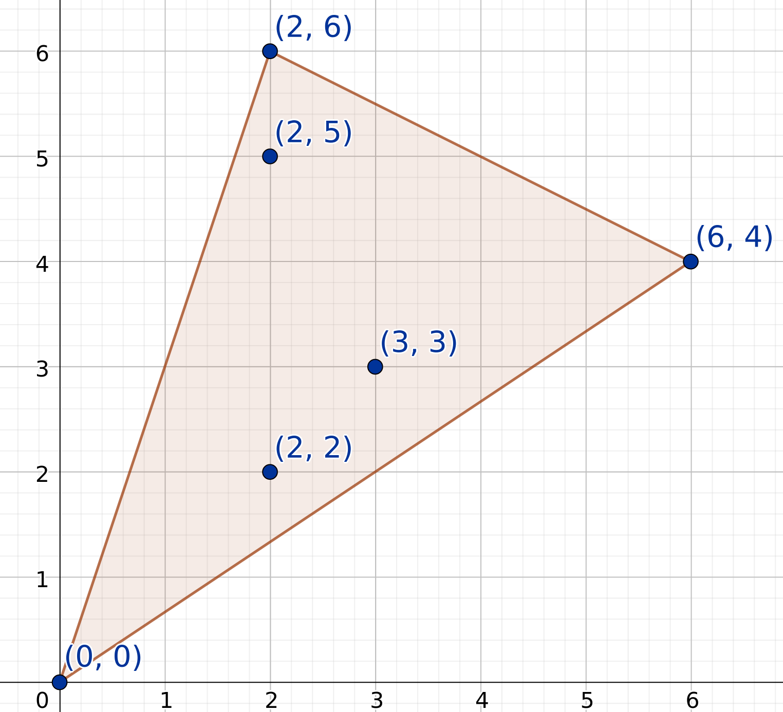
Figure 1: Exponents and the Newton polytope of the polynomial $f(x_{1},x_{2})=x_{1}^{6}x_{2}^{4}+x_{1}^{3}x_{2}^{3}+x_{1}^{2}x_{2}^{6}+x_{1}^{2}x_{2}^{5}+x_{1}^{2}x_{2}^{2}+1$.

Figure 1 shows points corresponding to the exponents of the polynomial $f(x_{1},x_{2})=x_{1}^{6}x_{2}^{4}+x_{1}^{3}x_{2}^{3}+x_{1}^{2}x_{2}^{6}+x_{1}^{2}x_{2}^{5}+x_{1}^{2}x_{2}^{2}+1$. The coloured region represents the Newton polytope. Since the vertices $(6,4)$, $(2,6)$ and $(0,0)$ are even, correspond to terms with positive coefficients and are affinely independent, $f(x_{1},x_{2})$ is an ST-polynomial. Exponents of the inner terms $(2,5)$, $(3,3)$ and $(2,2)$ can be expressed as unique convex combinations of the vertices.

It is possible to split an ST-polynomial into circuit polynomials by taking the same Newton polytope for each inner term and splitting the coefficients of the monomial squares among the circuit polynomials. The existence of such a decomposition is a proof of nonnegativity.

Theorem 2.

([Lower, Theorem 3.1]) An ST-polynomial $f(\mathbf{x})$ is a SONC polynomial if for every $(\beta,\alpha)\in\Delta(f)\times V(f)$ there exist $a_{\beta,\alpha}\geq 0$ such that

$$\rvert f_{\beta}\rvert\leq\prod_{\alpha\in nz(\beta)}\left(\frac{a_{\beta,\alpha}}{\lambda_{\alpha}^{(\beta)}}\right)^{\lambda_{\alpha}^{\beta}},$$

$$f_{\alpha}\geq\sum_{\beta\in\Delta(f)}a_{\beta,\alpha}.$$

These $a_{\beta,\alpha}$ are the weights in the following SONC decomposition:

$$f(\mathbf{x})=\sum_{\beta\in\Delta(f)}\left(\sum_{\alpha\in nz(\beta)}a_{\beta,\alpha}\mathbf{x}^{\alpha}+f_{\beta}\mathbf{x}^{\beta}\right),$$

where $nz(\beta)$ denotes all exponents $\alpha\in V(f)$ that correspond to nonzero barycentric coordinates $\lambda_{\alpha}^{(\beta)}$.

3 Polynomial Optimization via SONC

In this section we restate known results on SONC polynomials and optimization methods based on SONC relaxations. Polynomial optimization problems can be stated as nonnegativity problems, since one can write the problem of minimizing $f(\mathbf{x})$ equivalently as

$$\sup\{\gamma\in\mathbb{R}:\hskip 5.69054ptf(\mathbf{x})-\gamma\geq 0\}.$$ (7)

This problem, however, is as hard as the original problem. Requiring instead that some certificate of nonnegativity exists for $f(\mathbf{x})-\gamma$ results in a relaxation of the original problem. If a SONC decomposition is used as a nonnegativity certificate, then the relaxation is

$$\sup\{\gamma\in\mathbb{R}:f(\mathbf{x})-\gamma\text{ is SONC}\}.$$ (8)

3.1 Lower Bounds for Unconstrained Optimization over an ST-Polynomial

This section shows how to write the problem of finding the optimal SONC decomposition of an unconstrained polynomial optimization problem as a convex optimization problem. We begin by recalling the notion of geometric programs (GPs).

Definition 4.

[BoydVan] A monomial is defined as a function $q:\mathbb{R}^{n}\rightarrow\mathbb{R}$ of the form $q(\mathbf{x})=cx_{1}^{a_{1}}\cdot\ldots\cdot x_{n}^{a_{n}}$ with $c>0$. A posynomial is defined as a sum of monomials. A geometric program (GP) is an optimization problem of the form p_0(x) p_i(x)≤1,   for i=1,…,r q_j(x)= 1,   for j=1,…,s, where $p_{0},\ldots,p_{r}$ are posynomials and $q_{1},\ldots,q_{s}$ are monomials.

Applying a logarithmic transformation to a GP results in a convex optimization problem [boyd2007tutorial] which is equivalent to the GP; in particular, applying a reverse transformation to an optimal solution of the transformed problem gives an optimal solution of the original GP.

Let $f$ be an ST-polynomial and assume that $\Delta(f)\cap\text{MoSq}(f)=\emptyset$. This can be achieved by disregarding all monomial squares that are not vertices of New$(f)$. This change preserves the validity of a lower bound on the optimal solution $f^{*}$ since monomial squares are always nonnegative [GP]. The following theorem formulates a GP based on the nonnegativity conditions from Theorem 2.

Theorem 3.

[GP, Corollary 2.7] Let $f$ be an ST-polynomial and introduce variables $a_{\beta,\alpha}>0$ for every $\beta\in\Delta(f)$ and $\alpha\in V(f)$. Then the SONC lower bound on $f$ is given by $f_{\text{SONC}}=f_{0}-\gamma$, where $\gamma$ is the solution of the following GP: ∑_β∈Δ(f)λ_0^(β) ≠0 λ_0^(β) ⋅—f_β —^1λ0(β) ⋅∏_j ∈nz(β) α≠0 (λα(β)aβ,α )^λα(β)λ0(β) ∑_β∈Δ(f) aβ,αfα≤1 for all α∈V(f) ∖0 —f_β —∏_α∈nz(β) ( λα(β)aβ,α )^λ_α^(β)≤1 for all β∈Δ(f) with λ_0^(β)=0.

3.2 Lower Bounds for Constrained Optimization with an ST-Polynomial Lagrangian Function

Dressler et al. [GP] extend the method described above to the constrained case by utilizing Lagrangian relaxations. Consider an optimization problem of the form (1). Then the Lagrangian function of the problem has the form

$$L\left(\mathbf{x},\mathbf{\mu}\right)=f\left(\mathbf{x}\right)-\sum_{i=1}^{m}\mu_{i}g_{i}\left(\mathbf{x}\right),$$ (9)

where $\mu_{i}\geq 0$, $i=1,\ldots,m$ are Lagrangian multipliers. Let $\mu_{0}:=1$ and $g_{0}:=-f$. The Lagrangian then becomes

$$L(\textbf{x},\mathbf{\mu})=-\sum_{i=0}^{m}\mu_{i}g_{i}(\mathbf{x}).$$ (10)

The coefficients of the polynomial (10) depend on $\mu$, and term cancellation may lead to some of the monomials vanishing for certain values of $\mu$. Therefore, the definitions of exponent sets need to account for this. Thus, the support $\mathcal{A}(L)$ is defined as the union of supports of individual polynomials defining the objective and the constraints: $\mathcal{A}(L)=\cup_{i=0}^{m}\mathcal{A}(g_{i})$. The definitions of the vertices of the Newton polytope and the exponents corresponding to inner terms are analogous: $V(L)=\cup_{i=0}^{m}V(g_{i})$ and $\Delta(L)=\cup_{i=0}^{m}\Delta(g_{i})$.

We assume that $\Delta(L)$ does not contain exponents corresponding to monomial square terms. If this is not the case, then, since monomial square terms are always nonnegative, we can disregard monomial square inner terms and still obtain a valid lower bound.

Further, we assume that $L$ is an ST-polynomial, and write it in the form

$$L(\mathbf{x},\mathbf{\mu})=\sum_{\alpha\in V(L)}L(\mathbf{\mu})_{\alpha}\mathbf{x}^{\alpha}+\sum_{\beta\in\Delta(L)}L(\mathbf{\mu})_{\beta}\mathbf{x}^{\beta}.$$ (11)

For a fixed $\mu$, the problem of optimizing the Lagrangian reduces to a similar GP that is solved in the unconstrained case. Let $\gamma(\mu)$ denote the optimal value of problem (3) for a given $\mu$. The goal is to find the best possible lower bound $\gamma^{*}$ over all nonnegative $\mu$, that is, $\gamma^{*}=\sup\{\gamma(\mu):\mu\in\mathbb{R}^{n}_{+}\}$. However, directly writing this in the form (3) does not produce a GP, and additional relaxation steps are necessary in order to obtain a GP [GP].

As before, let $\lambda_{\alpha}^{(\beta)}$ denote the barycentric coordinates for each $\beta\in\Delta(L)$ with respect to the vertices $\alpha\in V(L)$. For each $\beta\in\Delta(L)$, we introduce new variables $a_{\beta,\alpha}>0$ for each $\alpha\in V(L)$, and $b_{\beta}\geq 0$. For each constraint $g_{i}(\mathbf{x})$, $i=1,\ldots,m$, we denote by $g_{i,\alpha}$ the coefficient corresponding to the monomial $\mathbf{x}^{\alpha}$. Then optimizing the Lagrangian over $\mu$ and $\mathbf{x}$ is equivalent to solving the following optimization problem with variables $\mathbf{\mu}$, $a_{\beta}$ and $b_{\beta}$: μ≥0, a_β ¿ 0, b_β ≥0∑_i=1^m μ_i g_i,0 + ∑_β∈Δ(L)λ_0^(β) ≠0 λ_0^(β) ⋅b_β^1λ0(β) ⋅∏_