Review of ensemble gradients for robust optimisation

Abstract

In robust optimisation problems the objective function consists of an average over (an ensemble of) uncertain parameters. Ensemble optimisation (EnOpt) implements steepest descent by estimating the gradient using linear regression on Monte-Carlo simulations of (an ensemble of) control parameters. Applying EnOpt for robust optimisation is costly unless the evaluations over the two ensembles are combined, i.e. ‘paired’. Here, we provide a new and more rigorous perspective on the stochastic simplex approximate gradient (StoSAG) used in EnOpt, explaining how it addresses detrimental cross-correlations arising from pairing by only capturing the variability due to the control vector, and not the vector of uncertain parameters. A few minor variants are derived from a generalized derivation, as well as a new approach using decorrelation. These variants are tested on linear and non-linear toy gradient estimation problems, where they achieve highly similar accuracy, but require a very large ensemble size to outperform the non-robust approach when accounting for variance and not just bias. Other original contributions include a discussion of the particular robust control objectives for which EnOpt is suited, illustrations, a variance reduction perspective, and a discussion on the centring in covariance and gradient estimation.

1 Introduction

Ensemble methods are particularly skilled for estimation and control problems involving dynamics that are nonlinear, high-dimensional, and computationally demanding, e.g. fluid dynamics. In data assimilation, the most prominent ensemble method is the ensemble Kalman filter (EnKF, Evensen, 1994), or some iterative version of it (Bocquet and Sakov, 2014). The EnKF resembles the unscented Kalman filter (Julier and Uhlmann, 2004), but places a larger emphasis on using a reduced number of members, or particles, and is usually complemented with techniques such as localisation to compensate for the limited sample size. In history matching and inverse problems it is the iterative ensemble smoother (EnRML or IES, Oliver, 1996; Raanes et al., 2019). In robust control problems it is ensemble optimisation (EnOpt, Chen et al., 2009, hereafter Chen09), our focus here. Common to all of these ensemble methods is that they combine (non-invasive and embarrassingly parallelizable) Monte-Carlo simulations with linear least-squares (LLS) regression to estimate derivatives which are generally not readily available.

1.1 Iterative convergence in the presence of stochasticity

Being that it uses a stochastic gradient for steepest descent/ascent, EnOpt may be said fall in the category of stochastic approximation (SA, Robbins and Monro, 1951), whose main result is a stochastic form of the contraction theorem: even if we only have access to noisy, i.e. stochastic, function evaluations, fixed-point iterations may converge, providing the noise is unbiased and bounded, and that the step length goes to zero at a specific rate. Kiefer and Wolfowitz (1952) applied this result for optimisation by considering the first-order, central finite difference approximations for the gradient of an objective which again can only be evaluated subject to noise, The cost of the evaluations required by this finite-difference stochastic approximation (FDSA) may be offset by parallelisation, but can be significant.

By contrast, the simultaneous perturbation stochastic approximation method Spall et al. (SPSA 1992) uses only a single perturbation for its finite difference approximation, only checking which of the two opposite directions are uphill or downhill, similarly to the method of coordinate descent. SPSA generally converges at a slower rate than FDSA, but at a lower cost. Since the perturbation direction changes with each iteration, some convergence results can be proven (Bhatnagar et al., 2013, §5.2.3).

EnOpt may be said to fall somewhere in between FDSA and SPSA, since we are generally free to choose the size of the ensemble of controls to which LLS regression is applied. Thus, despite the gradient estimates being stochastic and not exploring all directions at each iteration, we have some confidence that convergence may be achieved in fairly general circumstances. The remainder of this paper is not concerned iterative convergence, focusing instead on the accuracy of the gradient estimates for a given ensemble.

1.2 Outline

Section 2 begins by a discussion of covariance estimation and centring strategies, which is complemented by appendix A. We then define the fundamental regression estimator, linking regression to average, analytic derivatives, illustrating that it effectively blurs the objective (or cost) function, and discussing common preconditioning techniques. Section 3 continues the introduction, detailing the type of problem at which EnOpt excels, namely robust control problems where the objective function involves computationally demanding simulations. This specialised skill is largely due, as described in section 4, to the cost-saving technique of Chen09 called ‘pairing’, and the refinement thereof of Fonseca et al. (2014) called StoSAG, which greatly improves its accuracy.

We think that a clear derivation of StoSAG is missing from the literature, as discussed in appendix B, and that the surrounding theory can be clarified, which is our main purpose and original contribution. Our first explanation of the refinement is presented in section 5, which is complemented by a variance reduction perspective in appendix C, and a linear example in appendix D. Section 6 derives some minor variations on the StoSAG gradient estimate, all of which are experimentally compared in section 7.

2 Fundamental ensemble gradient

An ensemble is a sample for which each realisation, or member, ${\bm{u}}_{n}\in\mathbb{R}^{d_{{\bm{u}}}}$, for $n=1,\ldots,N$, is assumed an independent draw from the same probability distribution, $p({\bm{u}})$.

2.1 Covariance estimation and centring

Denote $\bar{{\bm{u}}}=\frac{1}{N}\sum_{n}{\bm{u}}_{n}$ the sample mean, where the summation bounds are left implicit. Consider the cross-covariance of ${\bm{u}}$ with the generic function ${\bm{f}}:\mathbb{R}^{d_{{\bm{u}}}}\rightarrow\mathbb{R}^{d_{{\bm{f}}}}$, denoted ${\mathbf{{C}}}_{{\bm{f}},{\bm{u}}}\in\mathbb{R}^{d_{{\bm{f}}}\times d_{{\bm{u}}}}$. For $N\geq 2$, an unbiased estimate is

$$\bar{{\mathbf{{C}}}}_{{\bm{f}},{\bm{u}}}\coloneqq\frac{1}{N-1}\sum_{n}{\bm{f}}({\bm{u}}_{n})\,({\bm{u}}_{n}-\bar{{\bm{u}}})^{{\mathsf{T}}}\,,$$ (1)

where vectors have column orientation by default. Note that, for any $c$ constant in $n$, $\sum_{n}c\,({\bm{u}}_{n}-\bar{{\bm{u}}})={\bm{0}}$, so that the explicit centring of ${\bm{f}}({\bm{u}}_{n})$ in equation 1 by subtracting its sample mean, $\frac{1}{N}\sum_{n}{\bm{f}}({\bm{u}}_{n})$, can be omitted.

Unlike the data assimilation setting, the true mean of the input, ${\bm{u}}$, denoted ${\bm{\mu}}$, is known in EnOpt. Therefore it is possible to estimate ${\mathbf{{C}}}_{{\bm{f}},{\bm{u}}}$, even for $N=1$, by

$$\frac{1}{N}\sum_{n}{\bm{f}}({\bm{u}}_{n})({\bm{u}}_{n}-{\bm{\mu}})^{{\mathsf{T}}}\,.$$ (2)

Even though ${\bm{f}}({\bm{u}}_{n})$ does not get subtracted by the (unknown) true mean of the output, $\operatorname{\mathbb{E}}{\bm{f}}({\bm{u}})$, the estimate (2) is also unbiased, since $\operatorname{\mathbb{E}}b\,({\bm{u}}_{n}-{\bm{\mu}})={\bm{0}}$ for any constant $b$. Nevertheless, despite the seeming benefit of ${\bm{\mu}}$ over $\bar{{\bm{u}}}$, the estimate of expression (2) generally has a higher variance than $\bar{{\mathbf{{C}}}}_{{\bm{f}},{\bm{u}}}$ of equation 1. This is proven for linear ${\bm{f}}$ in appendix A, whose analysis also suggests approximately centring ${\bm{f}}({\bm{u}}_{n})$ in expression (2) by subtracting ${\bm{f}}({\bm{\mu}})$, even though ${\bm{f}}({\bm{\mu}})\neq\operatorname{\mathbb{E}}{\bm{f}}({\bm{u}})$ unless ${\bm{f}}$ is linear.

However, in our numerical tests (not shown), the lowest variance is usually achieved if the input ensemble, $\{{\bm{u}}_{n}\}$, is centred before running the Monte-Carlo simulation altogether, such that $\bar{{\bm{u}}}={\bm{\mu}}$. Therefore, this operation will be tacitly assumed for the remainder of this manuscript.

Let ${\mathbf{{U}}}\in\mathbb{R}^{d_{{\bm{u}}}\times N}$ be the ensemble matrix, meaning that its $n$-th column is the $n$-th member, ${\bm{u}}_{n}$, and let $\tilde{{\mathbf{{U}}}}$ be the centred ensemble matrix, whose $n$-th column is the anomaly, or deviation, ${\bm{u}}_{n}-\bar{{\bm{u}}}$, where, we recall, $\bar{{\bm{u}}}={\bm{\mu}}$. Also extend the definition of ${\bm{f}}$ to allow matrix input by applying the original function to each column. Then the sample covariance matrix (1) may be written as

$$\bar{{\mathbf{{C}}}}_{{\bm{f}},{\bm{u}}}=\frac{1}{N-1}{\bm{f}}({\mathbf{{U}}})\,\tilde{{\mathbf{{U}}}}^{{\mathsf{T}}}\,.$$ (3)

2.2 Linear regression

For a given distribution of ${\bm{u}}$, the (exact) regression coefficient matrix of ${\bm{f}}$ is defined as ${\mathbf{{C}}}_{{\bm{f}},{\bm{u}}}\,{\mathbf{{C}}}_{{\bm{u}}}^{-1}$. For any $N\geq 2$, an estimate can be composed using the covariance estimator (3) and the (Moore-Penrose) pseudo-inverse as $\bar{\nabla}\!{\bm{f}}\coloneqq\bar{{\mathbf{{C}}}}_{{\bm{f}},{\bm{u}}}\,\bar{{\mathbf{{C}}}}_{{\bm{u}}}^{+}$. But, by the identity

$${\mathbf{{A}}}^{{\mathsf{T}}}({\mathbf{{A}}}{\mathbf{{A}}}^{{\mathsf{T}}})^{+}={\mathbf{{A}}}^{+}\,,$$ (4)

the regression estimate formula simplifies to

$$\bar{\nabla}\!{\bm{f}}={\bm{f}}({\mathbf{{U}}})\,\tilde{{\mathbf{{U}}}}^{+}\,.$$ (5)

The right-hand side can be recognised as the linear least squares (LLS) coefficient matrix, meaning that it minimises the sum of squared residuals among all linear approximations to ${\bm{f}}$. Assuming Gaussianity of the residuals makes it a maximum-likelihood (ML) estimate. Under other qualifying assumptions, it can also be termed BLUE, (U)MVUE, and minimum-norm LLS estimate.

Equation 5 is meant as a definition of the operator $\bar{\nabla}$. Since $\bar{\nabla}$ also entails Monte-Carlo simulations to generate ${\bm{f}}({\mathbf{{U}}})$, it may be useful to distinguish this notion from the more general LLS method, which relates any two samples, not necessarily computed via some ${\bm{f}}$, and we therefore call $\bar{\nabla}\!{\bm{f}}$ the ensemble (regression) gradient (or Jacobian). Gu and Oliver (2007) called $\bar{\nabla}\!{\bm{f}}$ the ensemble sensitivity matrix. Do and Reynolds (2013) also discussed the closely-related simplex gradient, the difference being that the deviations are not centred, but measured from a chosen reference point, typically, but not necessarily, ${\bm{\mu}}$ and ${\bm{f}}({\bm{\mu}})$.

2.3 Asymptotics and Stein’s lemma

Although both $\bar{{\mathbf{{C}}}}_{{\bm{{\bm{f}}}},{\bm{u}}}$ and $\bar{{\mathbf{{C}}}}_{{\bm{u}}}$ are unbiased, the ensemble regression gradient, $\bar{\nabla}\!{\bm{f}}$ of equation 5, does not generally have expectation ${\mathbf{{C}}}_{{\bm{f}},{\bm{u}}}\,{\mathbf{{C}}}_{{\bm{u}}}^{-1}$, unless ${\bm{f}}$ is linear and $N>d_{{\bm{u}}}$. Nevertheless, by Slutsky’s theorem, it is consistent, converging almost surely:

$$\bar{\nabla}\!{\bm{f}}\xrightarrow[N\rightarrow+\infty]{}{\mathbf{{C}}}_{{\bm{f}},{\bm{u}}}\,{\mathbf{{C}}}_{{\bm{u}}}^{-1}\,.$$ (6)

Now, suppose ${\bm{u}}$ is Gaussian, ${\bm{u}}\sim\mathcal{N}({\bm{\mu}},{\mathbf{{C}}}_{{\bm{u}}})$, whose density is denoted $p({\bm{u}})\propto\exp(-\|{\bm{u}}-{\bm{\mu}}\|^{2}_{{\mathbf{{C}}}_{u}}/2)$, and that ${\bm{f}}$ is a function with bounded gradient, $\nabla\!{\bm{f}}({\bm{u}})$. Then

$$\operatorname{\mathbb{E}}\nabla\!{\bm{f}}({\bm{u}})={\mathbf{{C}}}_{{\bm{f}},{\bm{u}}}\,{\mathbf{{C}}}_{{\bm{u}}}^{-1}\,,$$ (7)

which is known as Stein’s lemma (Stein, 1972). It may be shown by performing integration by parts for the expectation, followed by Stokes’ theorem and the fact that $p({\bm{u}})\rightarrow 0$ at infinity, followed by the “logarithm trick”, i.e. $\nabla p({\bm{u}})=p({\bm{u}})\nabla\!\log p({\bm{u}})$, where Gaussianity yields $\nabla\!\log p({\bm{u}})=-{\mathbf{{C}}}_{{\bm{u}}}^{-1}[{\bm{u}}-{\bm{\mu}}]$.

Equations 6 and 7 produce

$$\bar{\nabla}\!{\bm{f}}\xrightarrow[N]{}\operatorname{\mathbb{E}}\nabla\!{\bm{f}}({\bm{u}})\,,$$ (8)

which establishes a relationship from ensemble sensitivity to the actual gradient, motivating its use in optimisation contexts or perspectives. This is usually accomplished in the ensemble literature by inserting the leading-order Taylor expansion into the cross-covariance. However, the above approach by Stein’s lemma should be favoured because it (i) is exact, (ii) shows that errors cancel thanks to averaging, (iii) shows that the ‘target’ of the estimation is the average gradient – not the gradient at a point.

2.4 Implicit Gaussian blurring

Equation 8 was initially pointed out in the ensemble literature by Raanes et al. (2019). A similar result was found by Stordal et al. (2016) in terms of mutation gradient, $\nabla_{\!{\bm{\mu}}}\operatorname{\mathbb{E}}{\bm{f}}({\bm{u}})$, i.e. the gradient in a parameter of the distribution. The two are related by the fact that, for any density that can be written $p({\bm{u}})=p_{0}({\bm{u}}-{\bm{\theta}})$, meaning that ${\bm{\theta}}$ is a location parameter,

$$\nabla_{\!{\bm{\theta}}}\operatorname{\mathbb{E}}{\bm{f}}({\bm{u}})=\operatorname{\mathbb{E}}\nabla\!{\bm{f}}({\bm{u}})\,,$$ (9)

whose demonstration involves integration by parts as in equation 7, and requires that the kernel, $p_{0}$, be sufficiently decaying.

Figure 1: Steepest descent, using exact (analytic) gradient (left) and (asymptotic) ensemble gradient (right), illustrated on the Rastrigin objective, $\mathcal{L}({\bm{u}})=20+\sum_{i=1,2}\bigl{[}v_{i}^{2}-10\cos(2\pi v_{i})\bigr{]}$, with $v_{1}=2u_{1}$ introducing a degree of non-homogeneity and $v_{2}=u_{2}$. The objective is shown on the left as contour surfaces ranging from 0 to 154, displaying its many local minima. The contours on the right show the blurred objective function, ${\bm{\mu}}\mapsto\operatorname{\mathbb{E}}\mathcal{L}({\bm{u}})$, with ${\bm{u}}\sim\mathcal{N}({\bm{\mu}},{\mathbf{{I}}})$, which is what using the ensemble gradient implicitly optimises. Steps are taken as $0.012$ times the gradient (or its average), starting from $5$ different initial positions, shown as white disks; smaller steps cause the gradient descent with exact gradient to be stuck within horizontal layers. In practice, acceleration techniques (e.g. momentum) should be used, allowing for much smaller ensemble or larger system size.

Thus, if $\mathcal{L}:\mathbb{R}^{d_{{\bm{u}}}}\rightarrow\mathbb{R}$ is the objective to be minimised, gradient descent using $\bar{\nabla}\mathcal{L}$, i.e. EnOpt, can be said to optimise, with respect to ${\bm{\mu}}$, the smoothed, or ‘blurred’ objective function, so-called because it is a convolution with the Gaussian kernel. Optimisation of kernel-smoothed objectives were studied at least as early as Katkovnik and Yu (1972). However, a great advantage of the ensemble (regression) gradient is that the blurring takes place implicitly.

Gradient ascent being a local optimisation method, this implicit smoothing of the objective may well be beneficial – indeed even a prerequisite – if the objective possesses many local optima, as illustrated in Figure 1, and thus a reason not to use a very small ${\mathbf{{C}}}_{{\bm{u}}}$. Of course, in later iterations, and hopefully near a good optimum, one could decrease the blurring by decreasing ${\mathbf{{C}}}_{{\bm{u}}}$. This could be done with a predefined sequence of scaling values, by covariance matrix adaptation (CMA, Fonseca et al., 2015b), or by using the gradient with respect to ${\mathbf{{C}}}_{{\bm{u}}}$ (Stordal et al., 2016).

2.5 Preconditioning

Some authors prefer to step along a ‘search direction’ of $\bar{\nabla}\!\mathcal{L}\,{\mathbf{{C}}}_{{\bm{u}}}$ rather than the vanilla gradient estimate, $\bar{\nabla}\!\mathcal{L}$, itself. Here, note that $\bar{\nabla}\!\mathcal{L}\in\mathbb{R}^{1\times d_{{\bm{u}}}}$ is a row vector and that, in contrast with data assimilation, the covariance matrix, ${\mathbf{{C}}}_{{\bm{u}}}$, is known, and might even be small enough to keep in memory. Alternatively, some prefer $\bar{\nabla}\!\mathcal{L}\,\bar{{\mathbf{{C}}}}_{{\bm{u}}}=\bar{{\mathbf{{C}}}}_{\mathcal{L},{\bm{u}}}$ where the equality follows by the pseudo-inverse identity (4). This preference may be partly due to a reluctance to use pseudo-inversions, either for computational reasons or for fear of aggravating sampling errors. However, there is a sense in which sampling errors cancel out for $\bar{\nabla}\!\mathcal{L}\,{\mathbf{{C}}}_{{\bm{u}}}$, and not for $\bar{\nabla}\!\mathcal{L}\,\bar{{\mathbf{{C}}}}_{{\bm{u}}}$. Consider the simple case: $\mathcal{L}(u)=\alpha+\beta u$. Then $\bar{\nabla}\!\mathcal{L}\,C_{u}=\beta C_{u}$ exactly, which is not subject to sampling error, while $\bar{C}_{\mathcal{L},u}=\beta\bar{C}_{u}$ is. Either way, it is important to mind the potential practical need for truncating its singular value spectrum or applying Tikhonov regularisation, detailed in the experiments of section 7.

Chen09 justified the implicit inclusion of $\bar{{\mathbf{{C}}}}_{{\bm{u}}}$ (and by the same token, ${\mathbf{{C}}}_{{\bm{u}}}$) as a regularizing preconditioner for gradient descent. This claims was further substantiated by the natural gradient perspective of Stordal et al. (2016). Additionally, the design of Chen09 (and their sometimes ‘double’ application) of ${\mathbf{{C}}}_{{\bm{u}}}$ was used to promote smoothness in the resulting control vector. However, Fonseca et al. (2017, hereafter Fons17) cautioned that the design (e.g. correlation length) of ${\mathbf{{C}}}_{{\bm{u}}}$ may not be easy, and that truncation may complicate the picture.

A potential downside to $\bar{\nabla}\!\mathcal{L}\,{\mathbf{{C}}}_{{\bm{u}}}$ and $\bar{\nabla}\!\mathcal{L}\,\bar{{\mathbf{{C}}}}_{{\bm{u}}}$ is that the direction is no longer estimating the direction of steepest descent, making the algorithm less transparent. On the other hand it may be argued that cross-covariances do possess the essential quality of the gradient, namely that it (specifically, the signs of its elements) indicates which coordinate directions are uphill and downhill. Another clear advantage of $\bar{\nabla}\!\mathcal{L}\,{\mathbf{{C}}}_{{\bm{u}}}$ and $\bar{\nabla}\!\mathcal{L}\,\bar{{\mathbf{{C}}}}_{{\bm{u}}}$, similar to preconditioning with the actual Hessian, is that their units contain those of ${\bm{u}}$, and not its reciprocals, so that the magnitudes of the individual elements are likely better suited.

The question of whether and how to precondition will not be further discussed in this manuscript, which will focus on $\bar{\nabla}\!\mathcal{L}$ alone. However, all of the equations ending in a trailing $\tilde{{\mathbf{{U}}}}^{+}$ may be converted to the preconditioned form simply by replacing $\tilde{{\mathbf{{U}}}}^{+}$ with $\tilde{{\mathbf{{U}}}}^{{\mathsf{T}}}/(N-1)$, and most of the discussion is relevant for either choice, since the question of preconditioning seems independent of that of dealing with robust control (also called robust optimisation) problems.

3 Use in robust control

In robust optimisation the objective function takes the form of an average, i.e.

$$\mathcal{L}({\bm{u}})\coloneqq\frac{1}{M}\sum_{m}\ell({\bm{x}}_{m},{\bm{u}})\,,$$ (10)

where the conditional objective, $\ell:\mathbb{R}^{d_{{\bm{x}}}\times d_{{\bm{u}}}}\rightarrow\mathbb{R}$, is a function also of ${\bm{x}}\in\mathbb{R}^{d_{{\bm{x}}}}$, whose uncertainty is quantified by an ensemble (independent of that of ${\bm{u}}$) thereof, $\{{\bm{x}}_{m}\}$, where $m=1,\ldots,M$.

Generally, $\ell$ will consist of some utility function applied to the output of some simulator model for a given $({\bm{x}},{\bm{u}})$. For example, preference or net profit, or proximity to a desired, reference, outcome. The subject of constraints (Oguntola and Lorentzen, 2021, e.g.) is not considered, and the specifics of $\ell$ are not discussed herein. I.e. we view $\ell$ as a black box, except to say that EnOpt is mainly tailored for applications in which evaluations of $\ell$ are costly because it contains a simulation model which typically involves computational fluid dynamics. Indeed, the original application of EnOpt of Chen09 is petroleum production optimisation, where $\ell$ is the simulated production of a reservoir, ${\bm{x}}$ parametrises its geological uncertainty, and ${\bm{u}}$ are well operation control parameters. Other uses include minimising the wake effect in wind farm layout and operations, and climate geoengineering studies.

Average objectives like $\mathcal{L}$ are also common in statistical inference and machine learning. In our study, however, ${\bm{x}}_{m}$ is not merely a data point, for which $\ell({\bm{x}}_{m},{\bm{u}})$ measures the data mismatch given ${\bm{u}}$. Instead, ${\bm{x}}_{m}$ is an input to the simulator, i.e. a possible realisation of a model parameter (vector). This means that evaluating $\ell$ for different values of ${\bm{x}}$ is equally costly as for different values of ${\bm{u}}$. Therefore $M$, i.e. the number of realisations of ${\bm{x}}$, tends to be relatively small, usually somewhere between $10$ and $100$, prompting the utmost parsimony in the use of evaluations for different ${\bm{x}}$. For this reason, quasi-Monte-Carlo sampling strategies should be considered (Ramaswamy et al., 2020).

3.1 Analytic gradient

In classical steepest (i.e. gradient) descent, iterative, cumulative steps are taken along the direction of the gradient,

$$\nabla\!\mathcal{L}({\bm{u}})=\frac{1}{M}\sum_{m}\frac{\mathrm{\partial}{\ell}}{\mathrm{\partial}{{\bm{u}}}}({\bm{x}}_{m},{\bm{u}})\,,$$ (11)

at the current iterate, ${\bm{u}}$. The iteration index is not denoted, as we are only concerned with the accuracy of gradient estimates for any given iteration.

3.2 Plain EnOpt gradient

The analytic gradient, $\frac{\mathrm{\partial}{\ell}}{\mathrm{\partial}{{\bm{u}}}}$, is not generally available. Therefore, in basic EnOpt, the gradient is estimated by the LLS ensemble gradient (5), yielding

$$\bar{\nabla}\!\mathcal{L} =\frac{1}{M}\sum_{m}\ell({\bm{x}}_{m},{\mathbf{{U}}})\,\tilde{{\mathbf{{U}}}}^{+}$$ (12)

$$\xrightarrow[N]{}\operatorname{\mathbb{E}}\nabla\!\mathcal{L}({\bm{u}})\,,$$ (13)

where the second line follows from equation 8, and $\ell({\bm{x}}_{m},{\mathbf{{U}}})$ indicates the row vector whose $n$-th entry is $\ell({\bm{x}}_{m},{\bm{u}}_{n})$.

Since the ensemble ${\mathbf{{U}}}$ is random (and resampled at each iteration), the gradient estimate, $\bar{\nabla}\!\mathcal{L}$, is stochastic. This gives associations to stochastic gradient descent (SGD). However, in SGD, stochasticity generally arises from a different source: random sub-sampling of the data, $\{{\bm{x}}_{m}\}$, at each iteration, to lower costs, to form a subgradient based only on that subset. Moreover, analytic gradients are often available. The sub-sampling technique could also be employed with EnOpt, although the potential benefit seems less, given the relatively small size of $M$. Nevertheless, in the context of SPSA for robust reservoir production optimisation, Li et al. (2013); Jesmani et al. (2020) did find significant success with sub-sampling.

4 Using fewer evaluations

Computing the plain EnOpt gradient estimate, $\bar{\nabla}\!\mathcal{L}$ of equation 12, implies $M\times N$ costly evaluations, $\ell({\bm{x}}_{m},{\bm{u}}_{n})$.

4.1 The fragile (‘mean-model’) gradient

One possibility to effectively reduce $M$ to $1$ is to only evaluate the objective function at $\bar{{\bm{x}}}$, i.e.

$$\bar{\nabla}\ell_{|\bar{{\bm{x}}}} =\ell(\bar{{\bm{x}}},{\mathbf{{U}}})\,\tilde{{\mathbf{{U}}}}^{+}$$ (14)

$$\xrightarrow[N]{}\operatorname{\mathbb{E}}\nabla\ell_{|\bar{{\bm{x}}}}({\bm{u}})\,,$$ (15)

where the notation $\ell_{|\bar{{\bm{x}}}}$ indicates the partial function with ${\bm{x}}$ fixed at $\bar{{\bm{x}}}$. The drawback of the estimate $\bar{\nabla}\ell_{|\bar{{\bm{x}}}}$ is of course that it does not take into account the uncertainty in ${\bm{x}}$, in direct contrast to the express aim of EnOpt (12), and may be facetiously termed fragile.

4.2 The paired gradient

In the original formulation of EnOpt, inspired by Lorentzen et al. (2006) and Nwaozo (2006), Chen09 proposed ‘mixing’, or ‘coupling’, or pairing the two ensembles, meaning that the summation (i.e. averaging) inherent in the matrix product in equation 12, which operates over ${\bm{u}}_{n}$, is merged with that over ${\bm{x}}_{m}$. This requires equality of the sample sizes (or that they be divisible), and only uses $M=N$ evaluations for the gradient estimate,

$$\bar{\nabla}\!\mathcal{L}_{{\textnormal{{Paired}}}}=\ell({\mathbf{{X}}},{\mathbf{{U}}})\,\tilde{{\mathbf{{U}}}}^{+}\,,$$ (16)

where ${\mathbf{{X}}}$ is the ensemble matrix for $\{{\bm{x}}_{m}\}$. The left-hand side will be explained in section 5, and so should for now be considered merely a label.

In general, $\operatorname{\mathbb{E}}_{{\bm{u}}}\operatorname{\mathbb{E}}_{{\bm{x}}}{\bm{f}}({\bm{x}},{\bm{u}})=\operatorname{\mathbb{E}}_{{\bm{x}},{\bm{u}}}{\bm{f}}({\bm{x}},{\bm{u}})$ if ${\bm{x}}$ and ${\bm{u}}$ are independent of one another. Similarly,

$$\frac{1}{N}\sum_{n}\frac{1}{M}\sum_{m}{\bm{f}}({\bm{x}}_{m},{\bm{u}}_{n})\approx\frac{1}{N}\sum_{n}{\bm{f}}({\bm{x}}_{n},{\bm{u}}_{n})\,,$$ (17)

which becomes an exact equality upon taking the expectation. Stordal et al. (2016) applied this reasoning to the plain, unpaired estimate (12) and the paired estimate (16), both in their preconditioned form, to justify pairing. They also showed that they share the same, unbiased, expected value, namely $\operatorname{\mathbb{E}}\nabla\!\mathcal{L}({\bm{u}})\,{\mathbf{{C}}}_{{\bm{u}}}$. While the pseudo-inverses complicate the picture, similar reasoning may be applied for the non-preconditioned estimates, i.e. that the limit of $\bar{\nabla}\!\mathcal{L}_{{\textnormal{{Paired}}}}$ is indeed $\operatorname{\mathbb{E}}\nabla\!\mathcal{L}({\bm{u}})$.

4.3 The StoSAG gradient

Fonseca et al. (2014) proposed a ‘modified’ EnOpt gradient, renamed by Fons17 as stochastic simplex approximate gradient (StoSAG).

$$\bar{\nabla}\mathcal{L}_{{\textnormal{{StoSAG}}}}=\bigl{[}\ell({\mathbf{{X}}},{\mathbf{{U}}})-\ell({\mathbf{{X}}},{\bm{\mu}})\bigr{]}\,\tilde{{\mathbf{{U}}}}^{+}\,.$$ (18)

The second term appears to incur an extra $M$ evaluations of $\ell$. However, this is not actually an additional cost, since $\ell({\mathbf{{X}}},{\bm{\mu}})$ and its mean are normally computed before accepting the previous iterative step.

Since $\ell({\mathbf{{X}}},{\bm{\mu}})$ and $\tilde{{\mathbf{{U}}}}^{{\mathsf{T}}}$ are independent, and the expectation of $\tilde{{\mathbf{{U}}}}$ is zero, the preconditioned form of the estimator (18) is an unbiased estimator just like the paired estimator. Similarly, the limit of $\bar{\nabla}\mathcal{L}_{{\textnormal{{StoSAG}}}}$ is also $\operatorname{\mathbb{E}}\nabla\!\mathcal{L}({\bm{u}})$.

Concerning $M<\infty$, Fonseca et al. (2015a) and Fons17 have provided considerable empirical evidence of significant improvements in the estimate (18) versus (16). On the other hand there exists little theoretical motivation beyond using a different “weighting”. Fons17 did show StoSAG to be superior if ${\mathbf{{C}}}_{{\bm{u}}}$ is large. Appendix B argues that this conclusion is correct, but that their analysis is quite flawed. Our main objective is to show that the estimate (18) hopes to capture variation due to ${\bm{u}}$ only, which is why and how it improves on the estimate (16) of Chen09.

5 Decoupling the pairing

The words “pairing” and “coupling” evoke a deterministic relationship. Let us explicitly assume such a coupling, i.e. that ${\bm{x}}$ is a function of ${\bm{u}}$, i.e. ${\bm{x}}={\bm{\phi}}({\bm{u}})$. This assumption immediately yields the effect of merging the averaging in ${\bm{x}}$ and ${\bm{u}}$, as in equation 16, since $p({\bm{x}}|{\bm{u}})=\delta({\bm{x}}-{\bm{\phi}}({\bm{u}}))$ so that $\operatorname{\mathbb{E}}_{{\bm{x}},{\bm{u}}}f({\bm{x}},{\bm{u}})=\operatorname{\mathbb{E}}_{{\bm{u}}}f({\bm{\phi}}({\bm{u}}),{\bm{u}})$. Indeed, define

$$\mathcal{L}_{\textnormal{Paired}}({\bm{u}})\coloneqq\ell({\bm{\phi}}({\bm{u}}),{\bm{u}})\,,$$ (19)

and let ${\bm{\phi}}$ be such that it exactly maps each ${\bm{u}}_{n}$ to ${\bm{x}}_{n}$ for $n=1,\ldots,M$; one could for example use a spline interpolant. Then, since $\mathcal{L}_{\textnormal{{Paired}}}({\bm{u}}_{n})=\ell({\bm{x}}_{n},{\bm{u}}_{n})$ for all $n$, applying $\bar{\nabla}$ to $\mathcal{L}_{\textnormal{{Paired}}}$ recovers the paired gradient estimate (16) of Chen09.

5.1 The problem with pairing

By equation 8, $\bar{\nabla}\!\mathcal{L}_{\textnormal{{Paired}}}\xrightarrow[N]{}\operatorname{\mathbb{E}}\nabla\!\mathcal{L}_{\textnormal{{Paired}}}({\bm{u}})$. But

$$\nabla\!\mathcal{L}_{\textnormal{{Paired}}}=\frac{\mathrm{\partial}{\ell}}{\mathrm{\partial}{{\bm{u}}}}+\frac{\mathrm{\partial}{\ell}}{\mathrm{\partial}{{\bm{x}}}}\frac{\partial{\bm{x}}}{\partial{\bm{u}}}\,,$$ (20)

which is the total derivative. By contrast, the plain, unpaired EnOpt gradient (12) targets equation 13, i.e. $\frac{1}{M}\sum_{m}\operatorname{\mathbb{E}}\frac{\partial\ell}{\partial{\bm{u}}}({\bm{x}}_{m},{\bm{u}})$, which contains only the partial derivative, i.e. only the first term of equation 20, $\operatorname{\mathbb{E}}\frac{\mathrm{\partial}{\ell}}{\mathrm{\partial}{{\bm{u}}}}({\bm{\phi}}({\bm{u}}),{\bm{u}})$.

Thus, the introduction of the explicit coupling function, which enables the highly articulate tools of analytical calculus, shows that replacing $\mathcal{L}$ with $\mathcal{L}_{\textnormal{{Paired}}}$ introduces an error, represented by the second term of the right-hand side of equation 20. The following subsection corrects for the error, while the subsequent subsection takes the approach of preventing it. Both are analytically shown to work in the linear case in appendix D.

5.2 Correcting for the error

Here we try to compensate $\operatorname{\mathbb{E}}\frac{\mathrm{\partial}{\ell}}{\mathrm{\partial}{{\bm{x}}}}({\bm{\phi}}({\bm{u}}),{\bm{u}})\frac{\partial{\bm{x}}}{\partial{\bm{u}}}({\bm{u}})$ from $\bar{\nabla}\!\mathcal{L}_{\textnormal{{Paired}}}$ and equation 20. Note that this chained derivative is the gradient, evaluated at ${\bm{v}}={\bm{u}}$, of the partial, composite function ${\bm{v}}\mapsto\ell_{|{\bm{u}}}({\bm{\phi}}({\bm{v}}))$. Estimating its expected gradient by $\bar{\nabla}$ still leaves the fixing, subscripted ${\bm{u}}$ unset, whereas it should also be averaged out. But since a second sample average would imply $N^{2}$ evaluations, we instead make the approximation

$$\ell_{|{\bm{u}}}\approx\ell_{|{\bm{\mu}}}\,,$$ (21)

similar to the approximation of the fragile estimate (14), but hopefully less detrimental since is applies to the second(ary), corrective, term. In summary,

$$\mathcal{L}_{\textnormal{{StoSAG}}}:=\mathcal{L}_{\textnormal{{Paired}}}-\ell_{|{\bm{\mu}}}\circ{\bm{\phi}}\,,$$ (22)

and applying $\bar{\nabla}\!$ to $\mathcal{L}_{\textnormal{{StoSAG}}}$ recovers the gradient estimate (18) of Fons17.

5.3 Preventing the error (decorrelating)

Alternatively, one can eliminate $\bar{\nabla}\ell_{{\bm{\mu}}}({\bm{\phi}}({\bm{u}}))=\ell({\mathbf{{X}}},{\bm{\mu}})\,\tilde{{\mathbf{{U}}}}^{+}$, where we have again included the approximation of equation 21. To achieve this, project ${\mathbf{{U}}}$ (row-wise) onto the space orthogonal to the centred vector $\ell({\mathbf{{X}}},{\bm{\mu}})$, say ${\bm{\psi}}$. The projection is given by ${\mathbf{{U}}}^{\prime}={\mathbf{{U}}}-{\mathbf{{U}}}{\bm{\psi}}{\bm{\psi}}^{{\mathsf{T}}}/\|{\bm{\psi}}\|^{2}_{2}$, which we then translate and scale so as to have the same mean and variances as the original ${\mathbf{{U}}}$. The gradient is then simply estimated by the paired estimate (16), except with ${\mathbf{{U}}}^{\prime}$ in place of ${\mathbf{{U}}}$. A notable drawback of the projection is the potential loss of rank in case $M\leq d_{{\bm{u}}}$.

6 Generalised StoSAG

As mentioned, the approximation (17) may be used to justify the pairing of the gradient estimate (16). But it can also be used to argue contrarily: the fact that it is an approximation (for $N<\infty$) means that paired estimates are not equal to plain, unpaired estimates. Figure 2 illustrates two issues with pairing: fewer sample points are used, as intended, but additionally the sample points are no longer on a grid. By contrast, the ‘nested’ sampling of the left-hand side of equation 17, illustrated by the points in Figure 2 (a), is explicitly independent: the very same ensemble, $\{{\bm{u}}_{n}\}$, is identically repeated for each ${\bm{x}}_{m}$, which enables showing $\bar{{\mathbf{{C}}}}_{{\bm{x}},{\bm{u}}}={\mathbf{{0}}}$. Meanwhile, the sample covariance of the points on the right-hand side of equation 17, illustrated in either subfigure (b) or (c), almost surely contains sampling error, which make it seem like there is a dependence between ${\bm{x}}$ and ${\bm{u}}$.

Figure 2: Scatter plot of sample points used in the evaluation of $\ell({\bm{x}},{\bm{u}})$ in various EnOpt gradient estimates. The edges and circles indicate the points used to compute increments of $\ell$.

With Figure 2 in mind, the idea of StoSAG gradient is evident. It is illustrated in Figure 3, which shows three variants that will be developed below, all of which have $\bar{{\mathbf{{C}}}}_{{\bm{x}},{\bm{u}}}={\mathbf{{0}}}$.

Figure 3: Like Figure 2, but for two-sided, distributed ensemble gradients, generalizing StoSAG.

6.1 Swapping operators

Note that the plain, unpaired EnOpt gradient (12) may be expressed as

$$\bar{\nabla}\!\mathcal{L}=\frac{1}{M}\sum_{m}\bar{\nabla}\ell_{|{\bm{x}}_{m}}\,,$$ (23)

i.e., just like the case with the analytic gradient (11), the ensemble gradient (5) distributes over the average in ${\bm{x}}$. Thus, we can use a new sample of ${\bm{u}}$ for each ${\bm{x}}_{m}$, i.e. $\bar{\nabla}\ell_{|{\bm{x}}_{m}}=\ell({\bm{x}}_{m},{\mathbf{{U}}}_{m})\,\tilde{{\mathbf{{U}}}}_{m}^{+}$. Then, since ${\mathbf{{U}}}_{m}$ differs for each ${\bm{x}}_{m}$, we can make its size, $N_{m}$ (since it can vary with $m$), small without impoverishing the overall sampling of ${\bm{u}}$. In the following experiments, this estimator will be called average LLS gradient.

It should be noted that equation (12) of Fons17 implicitly takes advantage of equation 23 [their equation (25)], but this is not explicitly stated, nor is their equation (12) motivated except by a “change of notation”. Lastly, from our non-preconditioned starting point, the following additional modification is necessary before arriving at StoSAG.

6.2 Ratio averaging

A small $N_{m}$ necessarily yields significant sampling error; the pseudo-inversions likely exacerbates it, and causes a significant bias. Reversing the pseudo-inverse identity (4) yields

$$\bar{\nabla}\ell_{|{\bm{x}}_{m}}=\bar{{\bm{c}}}_{m}\,\bar{{\mathbf{{C}}}}_{{\bm{u}},m}^{+}\,,$$ (24)

where $\bar{{\mathbf{{C}}}}_{{\bm{u}},m}=\frac{1}{N_{m}-1}\tilde{{\mathbf{{U}}}}_{m}\tilde{{\mathbf{{U}}}}_{m}^{{\mathsf{T}}}$ is the $m$-th sample covariance, and similarly $\bar{{\bm{c}}}_{m}=\frac{1}{N_{m}-1}\ell({\bm{x}}_{m},{\mathbf{{U}}}_{m})\,\tilde{{\mathbf{{U}}}}_{m}^{{\mathsf{T}}}$. Now, to alleviate the issues of the pseudo-inversion, replace $\bar{{\mathbf{{C}}}}_{{\bm{u}},m}$ by its average, $\frac{1}{M}\sum_{m}\bar{{\mathbf{{C}}}}_{{\bm{u}},m}$, so that equation 23 becomes

$$\bar{\nabla}\!\mathcal{L}\approx\Bigl{(}\sum_{m}\bar{{\bm{c}}}_{m}\Bigr{)}\Bigl{(}\sum_{m}\bar{{\mathbf{{C}}}}_{{\bm{u}},m}\Bigr{)}^{+}\,.$$ (25)

In other words, the average of the ‘ratio’ (23) is replaced by the ratio of averages (25). This forms the generalised StoSAG ensemble gradient, for which different sampling strategies (all using $N_{m}=2$) are illustrated in Figure 3.

Since covariance estimates are themselves averages, it is tempting to also replace $\frac{1}{M}\sum_{m}\bar{{\bm{c}}}_{m}$, by the plain covariance estimate computed by pooling all of the sub-samples, and do likewise for the covariances. However, doing so would merge the averaging in ${\bm{u}}$ with that in ${\bm{x}}$, and indeed would just recover the paired gradient estimate (16) of Chen09. Alternatively, one can do so for the covariances alone, resulting in an estimator we call hybrid.

6.3 Using only two points

A particularly interesting case is $N_{m}=2$, in which case we denote the two columns of ${\mathbf{{U}}}_{m}$ by ${\bm{v}}_{m}$ and ${\bm{w}}_{m}$. Then, since $\tilde{{\mathbf{{U}}}}_{m}$ is centred, its two columns, $\tilde{{\bm{v}}}_{m}$ and $\tilde{{\bm{w}}}_{m}$, are symmetric about zero, i.e. $\tilde{{\bm{v}}}_{m}=-\tilde{{\bm{w}}}_{m}=({\bm{v}}_{m}-{\bm{w}}_{m})/2$, so that $\bar{{\mathbf{{C}}}}_{{\bm{u}},m}=\tilde{{\mathbf{{U}}}}_{m}\tilde{{\mathbf{{U}}}}_{m}^{{\mathsf{T}}}=\tilde{{\bm{v}}}_{m}\tilde{{\bm{v}}}_{m}^{{\mathsf{T}}}+\tilde{{\bm{w}}}_{m}\tilde{{\bm{w}}}_{m}^{{\mathsf{T}}}=2\tilde{{\bm{v}}}_{m}\tilde{{\bm{v}}}_{m}^{{\mathsf{T}}}$. Hence

$$\sum_{m}\bar{{\mathbf{{C}}}}_{{\bm{u}},m}=\frac{1}{2}({\mathbf{{V}}}-{\mathbf{{W}}})({\mathbf{{V}}}-{\mathbf{{W}}})^{{\mathsf{T}}}\,,$$ (26)

where the $m$-th columns of ${\mathbf{{V}}},{\mathbf{{W}}}\in\mathbb{R}^{d_{{\bm{u}}}\times M}$ are ${\bm{v}}_{m}$ and ${\bm{w}}_{m}$. Similarly,

$$\bar{{\bm{c}}}_{m}=\frac{1}{2}\bigl{[}\ell({\bm{x}}_{m},{\bm{v}}_{m})-\ell({\bm{x}}_{m},{\bm{w}}_{m})\bigr{]}\,({\bm{v}}_{m}-{\bm{w}}_{m})^{{\mathsf{T}}}\,,$$ (27)

whose sum in $m$ can be written as a matrix product similar to equation 26. Thus, equation 25 becomes

$$\bar{\nabla}_{\!{\textnormal{{Two-sided}}}}\,\mathcal{L}\coloneqq\Bigl{[}\ell({\mathbf{{X}}},{\mathbf{{V}}})-\ell({\mathbf{{X}}},{\mathbf{{W}}})\Bigr{]}({\mathbf{{V}}}-{\mathbf{{W}}})^{+}\,,$$ (28)

where we have again used the pseudo-inverse identity (4). In summary, in the case of $N_{m}=2$, we can write equation 25 in a manner reminiscent of the ensemble LLS gradient (5) as well as two-sided finite differences.

Also note that in this $N_{m}=2$ case, the pseudo-inverses, $\{\tilde{{\mathbf{{U}}}}_{m}^{+}\}$, in the average LLS gradient (23) are analytically available and so can be efficiently computed.

6.4 Using mirror points

An alternative to sampling $\{{\bm{w}}_{m}\}$ is to simply set ${\bm{w}}_{m}$ as the reflection of ${\bm{v}}_{m}$ about the mean, i.e. ${\bm{w}}_{m}-{\bm{\mu}}={\bm{\mu}}-{\bm{v}}_{m}$. This may be seen as a lightweight sampling strategy, in the vein of quasi-random or quasi-Monte-Carlo methods. Of course, covariance estimators should include a scaling of $1/2$ when using mirrored samples, but this effect cancels in equation 25.

With mirroring, both ${\bm{v}}_{m}$ and ${\bm{w}}_{m}$ may be written in terms of a single draw, say ${\bm{u}}_{m}$ (again), i.e. ${\mathbf{{V}}}={\bm{\mu}}+\tilde{{\mathbf{{U}}}}$ and ${\mathbf{{W}}}={\bm{\mu}}-\tilde{{\mathbf{{U}}}}$, where the $m$-th column of $\tilde{{\mathbf{{U}}}}$ is ${\bm{u}}_{m}-{\bm{\mu}}$, and the vector-matrix sum is understood appropriately. Thus, ${\mathbf{{V}}}-{\mathbf{{W}}}=2\tilde{{\mathbf{{U}}}}$, and

$$\bar{\nabla}_{\!{\textnormal{{Two-sided}}}}\,\mathcal{L}=\frac{1}{2}\Bigl{[}\ell({\mathbf{{X}}},{\bm{\mu}}{+}\tilde{{\mathbf{{U}}}})-\ell({\mathbf{{X}}},{\bm{\mu}}{-}\tilde{{\mathbf{{U}}}})\Bigr{]}\,\tilde{{\mathbf{{U}}}}^{+}\,.$$ (29)

6.5 Mirroring values

Finally, in view of the above symmetry, it particularly tempting to make the approximation

$$\ell({\mathbf{{X}}},{\bm{\mu}})\approx\frac{1}{2}\bigl{[}\ell({\mathbf{{X}}},{\bm{\mu}}{-}\tilde{{\mathbf{{U}}}})+\ell({\mathbf{{X}}},{\bm{\mu}}{+}\tilde{{\mathbf{{U}}}})\bigr{]}\,.$$ (30)

Solving equation 30 for $\ell({\mathbf{{X}}},{\bm{\mu}}{-}\tilde{{\mathbf{{U}}}})$, yields the reflection of $\ell({\mathbf{{X}}},{\bm{\mu}}{+}\tilde{{\mathbf{{U}}}})$ about $\ell({\mathbf{{X}}},{\bm{\mu}})$, and its substitution into equation 29 yields a one-sided variation, which is nothing but $\bar{\nabla}\!\mathcal{L}_{{\textnormal{{StoSAG}}}}$ (18).

The averaging in equation 30 recalls the method of Jeong et al. (2020) of “approximating the objective function values of unperturbed control variables using the values of perturbed ones”. However, mirroring avoids the complication of estimating clusters of $\{{\bm{u}}_{n}\}$ for subset averaging. Also recall that equation 25 may be applied with any $N_{m}\geq 2$, even differing with $m$ (Fonseca et al., 2015a), so that larger subsets may be used.

The main advantage of $\bar{\nabla}\!\mathcal{L}_{\textnormal{{StoSAG}}}$ is that it uses $\ell({\mathbf{{X}}},{\bm{\mu}})$, which is available from the previous step validation, whereas the true two-sided variants require evaluation an additional $N$ points. Of course, the true two-sided variants can approximate $\ell({\mathbf{{X}}},{\bm{\mu}})$ using $\ell({\mathbf{{X}}},{\mathbf{{V}}})$ and $\ell({\mathbf{{X}}},{\mathbf{{W}}})$ and, as shown in Figure 3, they yield the benefit of using twice as many values of ${\bm{u}}$ in computing the gradient.

Figure 4: Elements of the experiment.

7 Experimental comparison

Fonseca et al. (2015a) studied the accuracy of the (preconditioned) StoSAG gradient estimator on the Rosenbrock function, comparing it with the paired ensemble gradient. This section presents a related quantitative comparison, but including all of the various gradient estimators presented in this paper.

7.1 Description

The experiment consists of computing the various ensemble gradients of $\mathcal{L}({\bm{u}})=\sum_{i}\mathcal{H}(u_{i}+x_{i})$, where $\mathcal{H}$ is a given Hermite polynomial, $i=1,\ldots,5$ is the dimension index, ${\bm{u}}\sim\mathcal{N}({\bm{0}},{\mathbf{{I}}}/100)$, and ${\bm{x}}\sim\mathcal{N}([-2,\ldots,2]^{{\mathsf{T}}},{\mathbf{{I}}}/4)$, as illustrated in Figure 4.

The error of a gradient estimate is defined as the difference with the estimation target (“truth”), $\operatorname{\mathbb{E}}\nabla\!\mathcal{L}({\bm{u}})$. Each experiment is repeated $10^{6}$ times using different random seeds. The root-mean-square (RMS) error is then computed over the seeds. The bias magnitude is obtained by averaging the errors over the seed, and taking its absolute value. Subsequently, both bias and RMS error are averaged over the dimensions, $i$.

The pseudo-inverses are all computed using Tikhonov regularisation, which we found to be more robust than truncation. Specifically, a pseudo-inverse is computed via singular value decomposition, and instead of using the reciprocals of the singular values, $1/s_{i}$, the diagonal matrix consists of the elements $s_{i}/\bigl{(}s_{i}^{2}+(\lambda s_{1})^{2}\bigr{)}$, where $\lambda$ is the (tunable) regularisation parameter, and $s_{1}$ the largest singular value. A range of $\lambda$ is tried out, and only the best result of each method is retained.

For generality and sensitivity analysis, this is all repeated for a range of different ensemble sizes and for each Hermite polynomial from $0$ to $6$.

The experiments are coded in Python, using NumPy (Harris et al., 2020), SciPy (Virtanen et al., 2020), pandas (Wes McKinney, 2010), and Xarray (Hoyer and Hamman, 2017), and can be found in the supplementary materials of the paper.

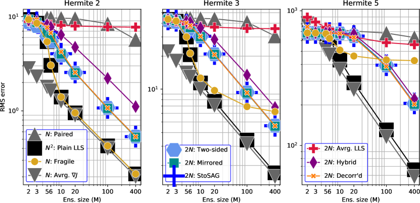
Figure 5: Root-mean-square error as a function of ensemble size for different ensemble gradient estimators. The panels show experiments using different Hermite polynomials, but all legends apply to all panels, with the number of evaluations of $\ell$ (i.e. $N$, $2N$, $N^{2}$) shown in front of their labels.

7.2 Results

The RMS errors are shown in Figure 5. As expected, the errors all increase from left to right across panels (notice the shifting y-axis), i.e. with increasing Hermite order (a proxy for nonlinearity), while they decrease inside each panel, i.e. for increasing ensemble size (on the x-axis). The average $\nabla\mathcal{L}$ (evaluated and averaged over the same ensemble as the other estimators) is uniformly the best. It is generally closely followed by the plain LLS gradient estimate, $\bar{\nabla}\mathcal{L}$ of equation 12, which uses $N^{2}$ evaluations, while the paired ensemble gradient, $\bar{\nabla}\mathcal{L}_{\!{\textnormal{{paired}}}}$ of equation 16, is nearly uniformly the worst.

The other methods generally score RMS errors somewhere in between these ‘baselines’, although simply taking the average of LLS ensemble gradients (red) performs very poorly. It can be seen that all of the StoSAG variants (blue), as well as the decorrelated approach (orange), perform almost equally well across the board. They appear to attain asymptotic convergence rates almost as soon as $N>5=d_{{\bm{u}}}$, in which setting the ensemble gradient is computed with a full-rank ensemble. The scores of the fragile (‘mean-model’) ensemble gradient (gold) undergoes a more precipitous drop around $N=6$, but flattens out for large ensemble sizes, since it is not a consistent estimator of $\operatorname{\mathbb{E}}\nabla\!\mathcal{L}({\bm{u}})$. However, for moderate ensemble sizes the StoSAG ensemble gradients are soundly outperformed by the fragile ensemble gradient, which means that, in terms of RMS error, their additional sampling error is more significant than the bias in the fragile gradient. The case of the 4th and 6th order Hermite polynomials (not shown) are similar to that of the 3rd and 5th, the general picture being that the higher the Hermite order is, the lower (but still high) $N$ is where the StoSAG and fragile score lines intersect.

Interestingly, for Hermite polynomial of degree $2$ (leftmost panel) the fragile gradient achieves equally good scores as the plain LLS ensemble gradient for all ensemble sizes, which is explained by the fact that in this case $\nabla\mathcal{L}$ is linear. In the case of the 1st order Hermite polynomial (not shown) the gradient is constant, and all of the methods are equally good, except for the paired ensemble gradient. In the case of the 0th order (constant, not shown) they all essentially achieve zero error.

The bias is shown in Figure 6. Here, the paired ensemble gradient does not demonstrate a markedly worse bias than StoSAG. Interestingly, the performance of the hybrid method (purple), where the covariance average is replaced by the total covariance, is actually slightly lower than for StoSAG, whereas in terms of RMS error it was slightly worse. The decorrelation method exhibit a somewhat higher bias than StoSAG. Most striking is that the fragile gradient has a very significant bias, explaining almost all of its RMS error.

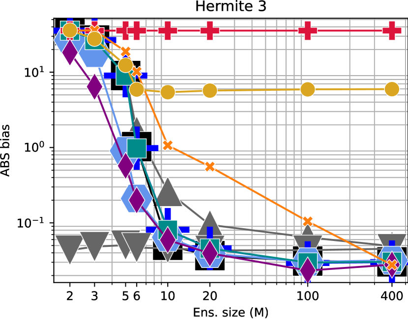
Figure 6: Like Figure 5 but for absolute bias (note: bias-minimising Tikhonov regularisation values generally differ from those used in Figure 5).

8 Summary

As detailed in the abstract and introduction, the aim of this paper has been to shed more light on the workings of the ensemble gradient in EnOpt; in particular its specialisation to robust control problems, and the importance of decoupling the partial derivatives, as is done by the StoSAG variant(s). The numerical experiments indicate that a very large ensemble size is needed for these robust ensemble gradient estimators to achieve lower errors than the fragile (‘mean-model’) estimator, albeit not in terms of bias.

Acknowledgements

This work has been funded by the Research Council of Norway under the CoRea project (grant number 301396), with some additional funding from Remedy (grant number 336240) We also thank Kjersti Solberg Eikrem for pointing out the possibility of centring by ${\bm{f}}({\bm{\mu}})$ in covariance estimation.

Appendix A Centring

We resume the discussion directly below equation 2. The reason its estimate usually has a larger variance than equation 1 is of course that equation 2 does not centre ${\bm{f}}({\bm{u}}_{n})$, by its sample mean, much less the true mean. Meanwhile, using the sample mean to centre ${\bm{f}}({\bm{u}}_{n})$ in equation 2 simply recovers $\bar{{\mathbf{{C}}}}_{{\bm{f}},{\bm{u}}}$, except scaled by $\frac{N-1}{N}$ which results in a bias.

Consider, for example, the simple case $f(u)=\beta$, for some constant $\beta$: equation 1 yields exactly $\bar{C}_{f,u}=0$, which has zero variance, while equation 2 produces $\beta(\bar{u}-\mu)$, which has variance $\beta C_{f,u}/N$.

In the linear case: $f(u)=\alpha u+\beta$, it can be shown that equation 1 yields $\bar{C}_{f,u}=\frac{\alpha}{N-1}\sum_{n}(u_{n}-\bar{u})^{2}$, while equation 2 produces $\frac{\alpha}{N}\sum_{n}(u_{n}-\mu)^{2}+(\alpha\mu-\beta)(\bar{u}-\mu)$.

Note that, in both cases, equation 2 produced the additional term $\eta\,(\bar{u}-\mu)$, where $\eta=\operatorname{\mathbb{E}}f(u)$, is the true (but unknown) mean of $f$, i.e. $\eta=\beta$ and $\eta=(\alpha\mu-\beta)$, respectively. Thus, unless $\eta$ happens to be sufficiently near zero, $\bar{{\mathbf{{C}}}}_{{\bm{f}},{\bm{u}}}$ of equation 1 will generally be less noisy lower than the estimate of equation 2.

Appendix B Comment on Fons17

As mentioned in section 4.3, Fons17 developed a theoretical error analysis of the preconditioned (i.e. cross-covariance) form of $\bar{\nabla}\!\mathcal{L}_{{\textnormal{{paired}}}}$ of Chen09  and $\bar{\nabla}\!\mathcal{L}_{\textnormal{{StoSAG}}}$ of Fonseca et al. (2014). However, there are a few issues, detailed below.

Firstly, their preoccupation with approximations (8) and (9) of Fons17, which Chen09 used in a Taylor development of the cross-covariance, is misplaced. Fons17 appears to make the odd claim that the approximation (9) of the average of $\ell$ by its evaluation at the average requires $\ell({\bm{x}}_{i},{\bm{u}})\approx\ell({\bm{x}}_{j},{\bm{u}})$ for any $i,j$, but it actually only requires a linear assumption. Moreover, Chen09 only used it for analysis, not for constructing the method, making its importance less “imperative”.

Actually, the main issue in the derivation of equation (14) of Chen09 is an unstated neglect of the variation in the uncertain parameters (following their substitution of the Taylor expansion). However, Fons17 appear to make a very similar omission: the second term on the right-hand side of their equation (28) is overlooked in the subsequent analysis. But this is the leading-order increment due to change in ${\bm{x}}$, and the fact that (all) increments due to variation in ${\bm{x}}$ are zero for StoSAG is the crucial difference.

Lastly, Fons17 derive the magnitudes of the errors of the cross covariance estimator, namely $\mathcal{O}{(\max_{n}\|{\bm{u}}_{n}-{\bm{\mu}}\|^{k})}$ with $k=3$ for the StoSAG gradient and only $k=1$ for the paired one. However, they do not comment on the fact that the cross-covariance itself scales with $\|{\bm{u}}-{\bm{\mu}}\|^{2}$. The root problem, moreover, is that a focus on individual (single-member) errors cannot hope to show that errors cancel by averaging, as pointed out in section 2.3.

Appendix C StoSAG as variance reduction

The principle of variance reduction can be stated as follows. Suppose we possess an estimate $a$, and some other random variable, $b$, whose mean is zero. As is well known,

$$\operatorname{\mathbb{V}{\textnormal{{ar}}}}(a-b)=\operatorname{\mathbb{V}{\textnormal{{ar}}}}(a)+\operatorname{\mathbb{V}{\textnormal{{ar}}}}(b)-2\operatorname{\mathbb{C}{\textnormal{{ov}}}}(a,b)\,.$$ (31)

Thus, while the mean is left unchanged, the variance of the ‘corrected’ estimate $a-b$ might be lower than that of $a$ if the covariance is sufficiently large. Indeed, rearranging equation 31 it can be seen that the improvement, $\operatorname{\mathbb{V}{\textnormal{{ar}}}}(a)-\operatorname{\mathbb{V}{\textnormal{{ar}}}}(a-b)$, is positive if the linear correlation of $a$ and $b$ satisfies $\rho\geq\frac{1}{2r}$, where $r\coloneqq\sqrt{\operatorname{\mathbb{V}{\textnormal{{ar}}}}(b)/\operatorname{\mathbb{V}{\textnormal{{ar}}}}(a)}$ is the ratio of the variances.

A variance reduction perspective was also considered by Stordal et al. (2016), based on Sun et al. (2009). However, they considered the design of a zero-mean $b$ so as to yield reduced variances. This is not generally possible, unless $\mathcal{L}$ has a simple expression, while empirical estimates were not found successful. By contrast, our purpose here is to use equation 31 to explain the success of the StoSAG gradient.

Let ${\bm{a}}=\bar{\nabla}\!\mathcal{L}_{\textnormal{{Paired}}}=\ell({\mathbf{{X}}},{\mathbf{{U}}})\tilde{{\mathbf{{U}}}}^{+}$ and ${\bm{a}}-{\bm{b}}=\bar{\nabla}\!\mathcal{L}_{\textnormal{{StoSAG}}}$, where the correction is ${\bm{b}}=\ell({\mathbf{{X}}},{\bm{\mu}})\,\tilde{{\mathbf{{U}}}}^{+}$. Note that indeed $\operatorname{\mathbb{E}}{\bm{b}}={\bm{0}}$, so that the subtraction of ${\bm{b}}$ does not alter the expected value. At the same time, ${\bm{b}}$ may well be expected to co-vary with ${\bm{a}}$, since they both contain ${\mathbf{{X}}}$. Therefore its subtraction from ${\bm{a}}$ should yield a reduction in variance.

Let us investigate this in the framework of equation 31. Since ${\bm{a}}$ and ${\bm{b}}$ are now vectors, the variances in equation 31 get replaced by covariance matrices, while $2\operatorname{\mathbb{C}{\textnormal{{ov}}}}(a,b)$ is replaced by $\operatorname{\mathbb{C}{\textnormal{{ov}}}}({\bm{a}},{\bm{b}})$ plus its transpose. Rephrasing the previous paraphrase, it seems reasonable (but we furnish no guarantees), that for most $\ell$, the correlation of $\ell({\mathbf{{X}}},{\mathbf{{U}}})$ and $\ell({\mathbf{{X}}},{\bm{\mu}})$ will be significantly positive ($\ell({\mathbf{{X}}},{\bm{\mu}})$ having correlation $1$ with itself, it difficult to see how replacing ${\bm{\mu}}$ with ${\mathbf{{U}}}$ would drastically lower it). Similarly, ${\bm{a}}$ and ${\bm{b}}$ should have significantly positive correlation. Thus, by equation 31, $\bar{\nabla}\!\mathcal{L}_{\textnormal{{StoSAG}}}$ should have a lower variance than $\bar{\nabla}\!\mathcal{L}_{\textnormal{{Paired}}}$.

By equation 31, the relative improvement $[\operatorname{\mathbb{V}{\textnormal{{ar}}}}(a)-\operatorname{\mathbb{V}{\textnormal{{ar}}}}(a-b)]/\operatorname{\mathbb{V}{\textnormal{{ar}}}}(a)$ is given by $r(2\rho-r)$. Thus, if the variance of ${\bm{x}}$ is small, then the variance of $\ell({\mathbf{{X}}},{\bm{\mu}})$ is small, so that the variance of ${\bm{b}}=\ell({\mathbf{{X}}},{\bm{\mu}})\,\tilde{{\mathbf{{U}}}}^{+}$ is often small, compared to that of ${\bm{a}}$. Hence $r$ is small and so is the relative improvement.

As an example, consider the bilinear conditional objective, $\ell({\bm{x}},{\bm{u}})={\bm{x}}+{\bm{u}}$, generalisable to higher dimensions by summing over the dimensions. In this linear case,

$$\bar{\nabla}\!\mathcal{L}_{\textnormal{{StoSAG}}}=({\mathbf{{X}}}+{\mathbf{{U}}})\,\tilde{{\mathbf{{U}}}}^{+}-({\mathbf{{X}}}+{\bm{\mu}}\mathds{1}^{{\mathsf{T}}})\,\tilde{{\mathbf{{U}}}}^{+}\,,$$ (32)

where the first and penultimate terms cancel, and $\mathds{1}^{{\mathsf{T}}}\tilde{{\mathbf{{U}}}}^{+}={\mathbf{{0}}}$, since $\tilde{{\mathbf{{U}}}}^{+}=\tilde{{\mathbf{{U}}}}^{{\mathsf{T}}}(\tilde{{\mathbf{{U}}}}\tilde{{\mathbf{{U}}}})^{+}$ is orthogonal to the vector of ones, $\mathds{1}$. This leaves only $\tilde{{\mathbf{{U}}}}\tilde{{\mathbf{{U}}}}^{+}$ which, if $N>d_{{\bm{u}}}$, is the centred identity matrix, which has zero variance. The same conclusion is provided by equation 31. In this case, the variances are equal, i.e. $r=1$, and $\rho=1$, so that the relative improvement is $1$. If $N\leq d_{{\bm{u}}}$, then $\tilde{{\mathbf{{U}}}}\tilde{{\mathbf{{U}}}}^{+}$ is a projection matrix (whose eigenvalues are all $0$ or $1$) whose subspace, reflecting the fact that not the entire space is sampled, is random. In either case, $\bar{\nabla}\!\mathcal{L}_{\textnormal{{StoSAG}}}$ yields a strong improvement on $\bar{\nabla}\!\mathcal{L}_{\textnormal{{Paired}}}$, which must also contend with the spurious noise of ${\mathbf{{X}}}\tilde{{\mathbf{{U}}}}^{+}$.

Appendix D Linear example

Consider the simple the bilinear conditional objective,

$$\ell({\bm{x}},{\bm{u}})=\sum_{i}({\mathbf{{A}}}{\bm{x}}+{\mathbf{{B}}}{\bm{u}})_{i}=\mathds{1}^{{\mathsf{T}}}({\mathbf{{A}}}{\bm{x}}+{\mathbf{{B}}}{\bm{u}})\,,$$ (33)

whose gradient is the constant $\frac{\mathrm{\partial}{\ell}}{\mathrm{\partial}{{\bm{u}}}}=\mathds{1}^{{\mathsf{T}}}{\mathbf{{B}}}$. Thus, the target, i.e. the average gradient, $\operatorname{\mathbb{E}}\nabla\!\mathcal{L}({\bm{u}})$, of equation 13, is also $\mathds{1}^{{\mathsf{T}}}{\mathbf{{B}}}$.

The paired ensemble gradient is

$$\bar{\nabla}\!\mathcal{L}_{\textnormal{{Paired}}}=\mathds{1}^{{\mathsf{T}}}{\mathbf{{A}}}{\mathbf{{X}}}\tilde{{\mathbf{{U}}}}^{+}+\mathds{1}^{{\mathsf{T}}}{\mathbf{{B}}}({\mathbf{{U}}}\tilde{{\mathbf{{U}}}}^{+})\,.$$ (34)

But, providing $N-1\geq d_{{\bm{u}}}$, the rank of $\tilde{{\mathbf{{U}}}}$ is $d_{{\bm{u}}}$ and hence $\tilde{{\mathbf{{U}}}}\tilde{{\mathbf{{U}}}}^{+}={\mathbf{{I}}}$. Thus, since the rows of ${\mathbf{{U}}}-\tilde{{\mathbf{{U}}}}$ are orthogonal to those of $\tilde{{\mathbf{{U}}}}$, it follows by equation 4 that also ${\mathbf{{U}}}\tilde{{\mathbf{{U}}}}^{+}={\mathbf{{I}}}$. In summary, the error in $\bar{\nabla}\!\mathcal{L}_{\textnormal{{Paired}}}$ is simply $\mathds{1}^{{\mathsf{T}}}{\mathbf{{A}}}{\mathbf{{X}}}\tilde{{\mathbf{{U}}}}^{+}$, which can be seen to be due to the correlation between ${\mathbf{{X}}}$ and ${\mathbf{{U}}}$.

Meanwhile, as shown by (22), $\bar{\nabla}_{\!{\textnormal{{StoSAG}}}}\mathcal{L}$ subtracts $\bar{\nabla}(\ell_{|{\bm{\mu}}}\circ{\bm{\phi}})=\mathds{1}^{{\mathsf{T}}}{\mathbf{{A}}}{\mathbf{{X}}}\tilde{{\mathbf{{U}}}}^{+}+\mathds{1}^{{\mathsf{T}}}{\mathbf{{B}}}{\bm{\mu}}\mathds{1}^{{\mathsf{T}}}\tilde{{\mathbf{{U}}}}^{+}$. But since $\tilde{{\mathbf{{U}}}}$ is centred, equation 4 yields $\mathds{1}^{{\mathsf{T}}}\tilde{{\mathbf{{U}}}}^{+}={\bm{0}}$. Thus, StoSAG obtains the exact gradient.

Similarly, centring $\ell({\mathbf{{X}}},{\bm{\mu}})$ yields ${\bm{\psi}}=\mathds{1}^{{\mathsf{T}}}{\mathbf{{A}}}\tilde{{\mathbf{{X}}}}$. Thus, the null space of the decorrelated ${\mathbf{{U}}}^{\prime}$ contains $\mathds{1}^{{\mathsf{T}}}{\mathbf{{A}}}\tilde{{\mathbf{{X}}}}$, and substituting ${\mathbf{{U}}}^{\prime}$ for ${\mathbf{{U}}}$ in equation 34 eliminates the error.

References

- Bhatnagar et al. (2013) Bhatnagar, S., H. Prasad, and L. Prashanth. Stochastic Recursive Algorithms for Optimization. Springer London, 2013. doi: 10.1007/978-1-4471-4285-0.
- Bocquet and Sakov (2014) Bocquet, M. and P. Sakov. An iterative ensemble Kalman smoother. Quarterly Journal of the Royal Meteorological Society, 140(682):1521–1535, 2014. doi: 10.1002/qj.2236.
- Chen et al. (2009) Chen, Y., D. S. Oliver, and D. Zhang. Efficient ensemble-based closed-loop production optimization. SPE Journal, 14(04):634–645, 2009. doi: 10.2118/112873-PA.
- Do and Reynolds (2013) Do, S. T. and A. C. Reynolds. Theoretical connections between optimization algorithms based on an approximate gradient. Computational Geosciences, 17(6):959–973, 2013. doi: 10.1007/s10596-013-9368-9.
- Evensen (1994) Evensen, G. Sequential data assimilation with a nonlinear quasi-geostrophic model using Monte Carlo methods to forecast error statistics. Journal of Geophysical Research, 99:10–10, 1994. doi: 10.1029/94JC00572.
- Fonseca et al. (2014) Fonseca, R. M., A. S. Stordal, O. Leeuwenburgh, P. M. J. Van den Hof, and J. D. Jansen. Robust ensemble-based multi-objective optimization. In ECMOR XIV-14th European conference on the mathematics of oil recovery, volume 2014, pages 1–14. European Association of Geoscientists & Engineers, 2014. doi: 10.3997/2214-4609.20141895.
- Fonseca et al. (2015a) Fonseca, R. M., S. S. Kahrobaei, L. Van Gastel, O. Leeuwenburgh, and J. Jansen. Quantification of the impact of ensemble size on the quality of an ensemble gradient using principles of hypothesis testing. In SPE Reservoir Simulation Symposium. OnePetro, 2015a. doi: SPE-173236-MS.
- Fonseca et al. (2015b) Fonseca, R. M., O. Leeuwenburgh, P. M. J. Van den Hof, and J.-D. Jansen. Improving the ensemble-optimization method through covariance-matrix adaptation. SPE Journal, 20(01):155–168, 2015b. doi: SPE-163657-PA.
- Fonseca et al. (2017) Fonseca, R. M., B. Chen, J. D. Jansen, and A. Reynolds. A stochastic simplex approximate gradient (StoSAG) for optimization under uncertainty. International Journal for Numerical Methods in Engineering, 109(13):1756–1776, 2017. doi: 10.1002/nme.5342.
- Gu and Oliver (2007) Gu, Y. and D. S. Oliver. An iterative ensemble Kalman filter for multiphase fluid flow data assimilation. SPE Journal, 12(04):438–446, 2007. doi: 10.2118/108438-PA.
- Harris et al. (2020) Harris, C. R., K. J. Millman, S. J. van der Walt, R. Gommers, P. Virtanen, D. Cournapeau, E. Wieser, J. Taylor, S. Berg, N. J. Smith, R. Kern, M. Picus, S. Hoyer, M. H. van Kerkwijk, M. Brett, A. Haldane, J. F. del Río, M. Wiebe, P. Peterson, P. Gérard-Marchant, K. Sheppard, T. Reddy, W. Weckesser, H. Abbasi, C. Gohlke, and T. E. Oliphant. Array programming with NumPy. Nature, 585(7825):357–362, Sept. 2020. doi: 10.1038/s41586-020-2649-2. URL https://doi.org/10.1038/s41586-020-2649-2.
- Hoyer and Hamman (2017) Hoyer, S. and J. Hamman. xarray: N-D labeled arrays and datasets in Python. Journal of Open Research Software, 5(1), 2017. doi: 10.5334/jors.148. URL https://doi.org/10.5334/jors.148.
- Jeong et al. (2020) Jeong, H., A. Y. Sun, J. Jeon, B. Min, and D. Jeong. Efficient ensemble-based stochastic gradient methods for optimization under geological uncertainty. Frontiers in Earth Science, page 108, 2020. doi: 10.3389/feart.2020.00108.
- Jesmani et al. (2020) Jesmani, M., B. Jafarpour, M. C. Bellout, and B. Foss. A reduced random sampling strategy for fast robust well placement optimization. Journal of Petroleum Science and Engineering, 184:106414, 2020. doi: 10.1016/j.petrol.2019.106414.
- Julier and Uhlmann (2004) Julier, S. J. and J. K. Uhlmann. Unscented filtering and nonlinear estimation. Proceedings of the IEEE, 92(3):401–422, 2004.
- Katkovnik and Yu (1972) Katkovnik, V. Y. and K. O. Yu. Convergence of a class of random search algorithms. Automation and Remote Control, 33(8):1321–1326, 1972. doi: 10.1002/ZAMM.19890690119.
- Kiefer and Wolfowitz (1952) Kiefer, J. and J. Wolfowitz. Stochastic estimation of the maximum of a regression function. The Annals of Mathematical Statistics, pages 462–466, 1952. doi: 10.1214/aoms/1177729392.
- Li et al. (2013) Li, L., B. Jafarpour, and M. R. Mohammad-Khaninezhad. A simultaneous perturbation stochastic approximation algorithm for coupled well placement and control optimization under geologic uncertainty. Computational Geosciences, 17(1):167–188, 2013. doi: 10.1007/s10596-012-9323-1.
- Lorentzen et al. (2006) Lorentzen, R. J., A. Berg, G. Naevdal, and E. H. Vefring. A new approach for dynamic optimization of water flooding problems. In Intelligent Energy Conference and Exhibition. OnePetro, 2006. doi: 10.2118/99690-MS.
- Nwaozo (2006) Nwaozo, J. E. Dynamic optimization of a water flood reservoir. Master’s thesis, University of Oklahoma Norman, Oklahoma, 2006.
- Oguntola and Lorentzen (2021) Oguntola, M. B. and R. J. Lorentzen. Ensemble-based constrained optimization using an exterior penalty method. Journal of Petroleum Science and Engineering, 207:109165, 2021. doi: 10.1016/j.petrol.2021.109165.
- Oliver (1996) Oliver, D. S. On conditional simulation to inaccurate data. Mathematical Geology, 28(6):811–817, 1996. doi: 10.1007/BF02066348.
- Raanes et al. (2019) Raanes, P. N., A. S. Stordal, and G. Evensen. Revising the stochastic iterative ensemble smoother. Nonlinear Processes in Geophysics, 26(3):325–338, 2019. doi: 10.5194/npg-26-325-2019.
- Ramaswamy et al. (2020) Ramaswamy, K. R., R. M. Fonseca, O. Leeuwenburgh, M. M. Siraj, and P. M. J. Van den Hof. Improved sampling strategies for ensemble-based optimization. Computational Geosciences, 24(3), 2020. doi: 10.1007/s10596-019-09914-8.
- Robbins and Monro (1951) Robbins, H. and S. Monro. A stochastic approximation method. The Annals of Mathematical Statistics, pages 400–407, 1951. doi: 10.1214/aoms/1177729586.
- Spall et al. (1992) Spall, J. C. et al. Multivariate stochastic approximation using a simultaneous perturbation gradient approximation. IEEE Transactions on Automatic Control, 37(3):332–341, 1992. doi: 10.1109/9.119632.
- Stein (1972) Stein, C. A bound for the error in the normal approximation to the distribution of a sum of dependent random variables. In Proceedings of the Sixth Berkeley Symposium on Mathematical Statistics and Probability, Volume 2: Probability Theory. The Regents of the University of California, 1972.
- Stordal et al. (2016) Stordal, A. S., S. P. Szklarz, and O. Leeuwenburgh. A theoretical look at ensemble-based optimization in reservoir management. Mathematical Geosciences, 48(4):399–417, 2016. doi: 10.1007/s11004-015-9598-6.
- Sun et al. (2009) Sun, Y., D. Wierstra, T. Schaul, and J. Schmidhuber. Efficient natural evolution strategies. In Proceedings of the 11th Annual conference on Genetic and evolutionary computation, pages 539–546, 2009. doi: 10.48550/arXiv.1209.5853.
- Virtanen et al. (2020) Virtanen, P., R. Gommers, T. E. Oliphant, M. Haberland, T. Reddy, D. Cournapeau, E. Burovski, P. Peterson, W. Weckesser, J. Bright, S. J. van der Walt, M. Brett, J. Wilson, K. J. Millman, N. Mayorov, A. R. J. Nelson, E. Jones, R. Kern, E. Larson, C. J. Carey, İ. Polat, Y. Feng, E. W. Moore, J. VanderPlas, D. Laxalde, J. Perktold, R. Cimrman, I. Henriksen, E. A. Quintero, C. R. Harris, A. M. Archibald, A. H. Ribeiro, F. Pedregosa, P. van Mulbregt, and SciPy 1.0 Contributors. SciPy 1.0: Fundamental Algorithms for Scientific Computing in Python. Nature Methods, 17:261–272, 2020. doi: 10.1038/s41592-019-0686-2.
- Wes McKinney (2010) Wes McKinney. Data Structures for Statistical Computing in Python. In Stéfan van der Walt and Jarrod Millman, editors, Proceedings of the 9th Python in Science Conference, pages 56 – 61, 2010. doi: 10.25080/Majora-92bf1922-00a.