Reconstructing discrete measures from projections. Consequences on the empirical Sliced Wasserstein Distance.

Abstract

This paper deals with the reconstruction of a discrete measure $\gamma_{Z}$ on $\mathbb{R}^{d}$ from the knowledge of its pushforward measures $P_{i}\#\gamma_{Z}$ by linear applications $P_{i}:\mathbb{R}^{d}\rightarrow\mathbb{R}^{d_{i}}$ (for instance projections onto subspaces). The measure $\gamma_{Z}$ being fixed, assuming that the rows of the matrices $P_{i}$ are independent realizations of laws which do not give mass to hyperplanes, we show that if $\sum_{i}d_{i}>d$, this reconstruction problem has almost certainly a unique solution. This holds for any number of points in $\gamma_{Z}$. A direct consequence of this result is an almost-sure separability property on the empirical Sliced Wasserstein distance.

1 Introduction

In this note, we are interested in the following question: for a given discrete probability measure $\gamma_{Z}$ on $\mathbb{R}^{d}$, and $p$ linear transformations $P_{i}:\mathbb{R}^{d}\rightarrow\mathbb{R}^{d_{i}}$, can we characterize the set of probability measures on $\mathbb{R}^{d}$ with exactly the same images as $\gamma_{Z}$ through all of the maps $P_{i}$? Formally, this set writes

$$\mathcal{S}=\left\{\gamma\in\mathcal{P}(\mathbb{R}^{d})\ |\ \forall i\in\llbracket 1,p\rrbracket,\;P_{i}\#\gamma=P_{i}\#\gamma_{Z}\right\},$$ (RP)

where $P_{i}\#\gamma$ denotes the push-forward of $\gamma$ by $P_{i}$, i.e. the measure on $\mathbb{R}^{d_{i}}$ such that for any Borelian $A\subset\mathbb{R}^{d_{i}}$, $(P_{i}\#\gamma)(A)=\gamma(P_{i}^{-1}(A))$, and $\mathcal{P}(\mathbb{R}^{d})$ denotes the space of probability measures on $\mathbb{R}^{d}$. The set $\mathcal{S}$ is nonempty since it contains at least $\gamma_{Z}$. A natural underlying question is to know when we get uniqueness, i.e. when $\mathcal{S}=\{\gamma_{Z}\}$. Indeed, in this case $\gamma_{Z}$ can be exactly reconstructed from the knowledge of all the $P_{i}\#\gamma_{Z}$, which is why we refer to this problem as a reconstruction problem.

This reconstruction problem appears in many applied fields where a multidimensional measure is known only through a finite set of images or projections. This is the case for instance in medical or geophysical imaging problems such as tomography [7]. It is also strongly related to the separability properties of the empirical version of the Sliced Wasserstein distance [14, 1], which is frequently used in machine learning applications [11, 5, 16].

In our reconstruction problem, it is clear that if one of the $P_{i}$ is injective (which implies $d\leq d_{i}$), then $\mathcal{S}=\{\gamma_{Z}\}$, which is why we focus here on the cases where none of the $P_{i}$ is injective. We will also assume in this note that the $P_{i}$ are surjective and that all the $d_{i}$ are strictly smaller than $d$, since we can always replace $\mathbb{R}^{d_{i}}$ by the smaller subspace $\mathrm{Im}(P_{i})$. To the best of our knowledge, this problem has not been widely discussed in the literature, perhaps because of its apparent simplicity. A close and more discussed question is the one of the existence of probability measures $\gamma$ with marginal constraints [12, 4, 13]. Existence results for such couplings are known for some families of measures [10], or measures exhibiting some specific correlation structures [3]. However, in the general case, even if marginal constraints are compatible with each other, the existence of solutions is not always ensured [8].

Our study case is different, since the constraints are all obtained as push-forwards of an unknown $\gamma_{Z}$, and the central question is not existence but uniqueness of solutions. It is well known that a measure is uniquely determined by its projections on all lines of $\mathbb{R}^{d}$ (Cramer-Wold theorem [2]), and more generally by its projections on a set of subspaces as soon as they cover the whole space together [15]. For a finite number of directions and in the case of a discrete measure $\gamma_{Z}$, simple linear algebra shows that if the number $p$ of projections is large enough, we get $\mathcal{S}=\{\gamma_{Z}\}$. When the $P_{i}$ are projections on different hyperplanes for instance, Heppes showed in 1956 [9] that a discrete distribution of at most $n$ points $\gamma_{Z}=\frac{1}{n}\sum_{l=1}^{n}\delta_{z_{l}}$ is uniquely characterized by its projections $P_{i}\#\gamma_{Z}$ if the number $p$ of these projections is larger than $n+1$, and that simple counter-examples could be exhibited with only $p=n$ hyperplanes. More recent works [6] show that uniqueness can be ensured with less projections as soon as the set of points is known to belong to a specific quadratic manifold. These results are deterministic, they hold for every set of points and hyperplanes with the appropriate cardinality. In this paper, we add some stochasticity to the problem, and assume that the lines of the matrices $P_{i}$  are i.i.d. following a law $\mathbb{P}$ which does not give mass to hyperplanes. Under this assumption, we show that if $\sum_{i=1}^{p}d_{i}>d$, then $\mathbb{P}$-almost surely $\mathcal{S}=\{\gamma_{Z}\}$. This result is very different from the ones already present in the literature: it holds only a.s., but this permits a considerably weaker condition on the $P_{i}$, and the condition for the reconstruction surprisingly does not depend on the number of points.

2 Solutions of the Reconstruction Problem

In this section, we characterize the set $\mathcal{S}$ of solutions defined in RP depending on the set of linear maps $P_{i}$. We write $\gamma_{Z}=\sum_{l=1}^{n}b_{l}\delta_{z_{l}}$ with $Z=(z_{1},\cdots,z_{n})\in(\mathbb{R}^{d})^{n}$, and assume that all points are distinct ($k\neq j\Longrightarrow z_{k}\neq z_{j}$). The weights $(b_{l})\in(\mathbb{R}_{+}^{*})^{n}$ sum to one and are each nonzero.

As we shall see, given a discrete measure $\gamma_{Z}$ with $n$ points in dimension $d$, the Reconstruction Problem RP has a unique solution $\mathcal{S}=\{\gamma_{Z}\}$ almost-surely when drawing the linear maps $P_{i}$ randomly, and when the dimensions strictly exceed $d$, i.e. when $D:=d_{1}+\cdots+d_{p}>d$.

2.1 Computing Linear Push-Forwards of Discrete Measures

Characterizing $\mathcal{S}$ requires the following technical Lemma, which provides a geometrical viewpoint of the push-forward operation.

Lemma 1 (Linear push-forward formula).

Let $P\in\mathcal{M}_{h,d}(\mathbb{R})$ of rank $h\leq d$ and $B\subset\mathbb{R}^{h}$.

Then $P^{-1}(B)=P^{T}(PP^{T})^{-1}B+\mathrm{Ker}P$.

1 shows a visualization of the set $P^{T}(PP^{T})^{-1}B+\mathrm{Ker}P$, first where $B$ is comprised of two points of $\mathbb{R}^{2}$ and $\mathrm{Ker}P$ is a horizontal plane in 3D, and second with $B$ a measurable set of $\mathbb{R}^{2}$. This illustrates the ill-posedness of the problem when the dimension of the projections and number of projections is too small. In this case with $p=1,\;d=3$ and $d_{1}=2$, the condition $P^{-1}(A)=P^{-1}(B)$ leaves a degree of freedom, which we can visualize as the vertical axis here.

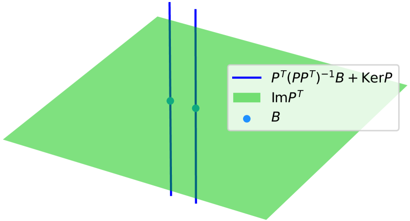
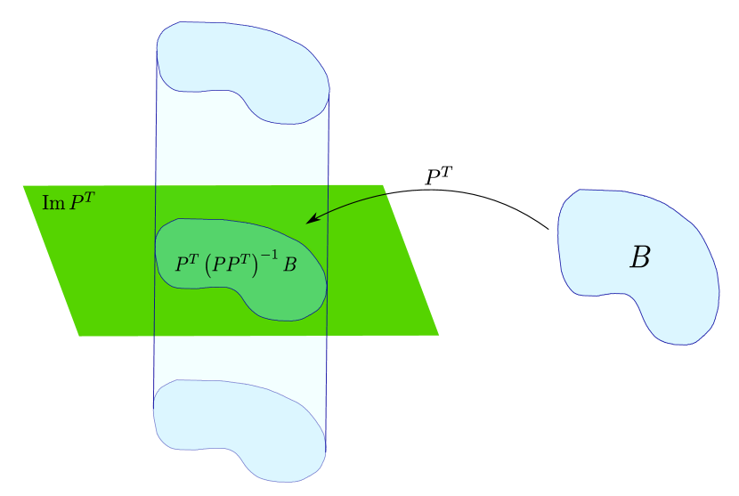
Figure 1: Illustrations of the linear push-forward formula $P^{-1}(B)$ for a 3D to 2D projection $P$, (left) when $B$ is a set of two points and (right) for a more general set $B$.

Proof.

If $a\in P^{T}(PP^{T})^{-1}B+\mathrm{Ker}P$, then by writing $a=P^{T}(PP^{T})^{-1}b+x$ with $b\in B$ and $x\in\mathrm{Ker}P$, we have $Pa=b\in B$, thus $a\in P^{-1}(B)$.

For the opposite inclusion, consider $a\in P^{-1}(B)$. Since $P$ is of full rank $h$, we have the decomposition $\mathbb{R}^{d}=\mathrm{Im}P^{T}\overset{\perp}{\bigoplus}\mathrm{Ker}P$, with $Q:=P^{T}(PP^{T})^{-1}P$ the orthogonal projection on $\mathrm{Im}P^{T}$.

Thus we can write $a=Qa+(I-Q)a=P^{T}(PP^{T})^{-1}Pa+(I-Q)a$. Since $Pa\in B$, we conclude that $a\in P^{T}(PP^{T})^{-1}B+\mathrm{Ker}P$. ∎

2.2 Restraining the support of solutions of RP

The following theorem states that the support of any solution of RP is constrained to a set $S$ obtained as the intersection of all sets $Z+\mathrm{Ker}P_{i}$. Without loss of generality, we will assume that each $P_{i}$ is of full rank $d_{i}$.

Theorem 1 (Support of solutions of RP).

If $\gamma$ is a solution of RP, then $\gamma\left(S\right)=1$ with

$$S:=\displaystyle\bigcap\limits_{i=1}^{p}\left(Z+\mathrm{Ker}P_{i}\right)=\displaystyle\bigcup\limits_{\begin{subarray}{c}(l_{1},\cdots,l_{p})\in\llbracket 1,n\rrbracket^{p}\end{subarray}}\quad\displaystyle\bigcap\limits_{i=1}^{p}\;\left(z_{l_{i}}+\mathrm{Ker}P_{i}\right).$$ (1)

Proof.

Using the same notations as in the proof of Lemma 1, we write $Q_{i}:=P_{i}^{T}(P_{i}P_{i}^{T})^{-1}P_{i}$ the orthogonal projection on $\mathrm{Im}P_{i}^{T}$ and we recall the decomposition $\mathbb{R}^{d}=\mathrm{Im}P_{i}^{T}\overset{\perp}{\bigoplus}\mathrm{Ker}P_{i}$. Thus, for any borelian $A$ of $\mathbb{R}^{d}$, $A\subset Q_{i}A+\mathrm{Ker}P_{i}$. Then $\gamma(A)\leq\gamma(Q_{i}A+\mathrm{Ker}P_{i})=P_{i}\#\gamma(P_{i}A)$, where the last equality is a direct consequence of Lemma 1.

Now, assume that $\gamma\in\mathcal{S}$ and define $S:=\displaystyle\bigcap\limits_{i=1}^{p}K_{i}$ with $K_{i}=Z+\mathrm{Ker}P_{i}$. For each $i$, applying the previous inequality to $K_{i}^{c}$ yields $\gamma(K_{i}^{c})\leq P_{i}\#\gamma(P_{i}K_{i}^{c})$. Since $\gamma$ is a solution, we have $P_{i}\#\gamma=P_{i}\#\gamma_{Z}$. By construction, $K_{i}=\{x,\;P_{i}x\in P_{i}Z\}$ thus $K_{i}^{c}=\{x,\;P_{i}x\notin P_{i}Z\}$. Since $P_{i}\#\gamma$ is supported by $P_{i}Z$, it follows that $P_{i}\#\gamma(P_{i}K_{i}^{c})=0$. Finally, $\gamma(S^{c})=\gamma(\displaystyle\bigcup\limits_{i=1}^{p}K_{i}^{c})\leq\sum_{i=1}^{p}\gamma(K_{i}^{c})=0$ and thus $\gamma(S)=1$.

∎

2 illustrates the previous result, with $p=2$ projections onto lines in $\mathbb{R}^{2}$, with $n=3$ points $Z=(z_{1},z_{2},z_{3})$. The support of any solution is confined to the intersections between any two lines of the form $z_{l}+\mathrm{Ker}P_{i}$. Here this corresponds to the intersecting points between an orange and a red line, allowing for 9 possible points, including the original 3. In this case any weighting of the 9 diracs that respect the marginal constraints will give a solution: there exists an infinity of possible solutions.

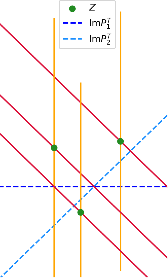
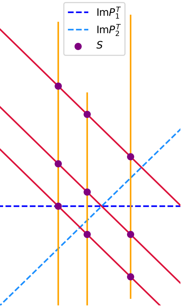
Figure 2: Illustration of the possible points for the support of a solution. On the left, $Z$ is the original measure points, and on the right, $S$ is the set of possible points for the support of a solution.

2.3 Conditions for unicity of solutions of RP

Leveraging the previous support restriction and elementary random affine geometry, we can further restrict the condition on the set of solutions $\mathcal{S}$. Theorem 2 below shows that if the random linear maps $P_{i}$ cover the original space $\mathbb{R}^{d}$ with redundancy (i.e. the sum of their target space dimensions strictly exceeds $d$), then almost surely, the reconstruction problem has a unique solution $\gamma_{Z}$. We formalize this random setting by the following assumption.

Assumption ($\mathcal{A}{P}$).

$$\quad\forall i\in\llbracket 1,p\rrbracket,\;P_{i}=\left(\begin{array}[]{ccc}\textrm{---}&\left(u_{i}^{(1)}\right)^{T}&\textrm{---}\\ \textrm{---}&\vdots&\textrm{---}\\ \textrm{---}&\left(u_{i}^{(d_{i})}\right)^{T}&\textrm{---}\end{array}\right)\quad\text{ where }u_{i}^{(j)}\sim\mathbb{P}\ \mathrm{i.i.d,}$$

where $\mathbb{P}$ is a probability distribution over $\mathbb{R}^{d}$ s.t. for any hyperplane $H\subset\mathbb{R}^{d},\;\mathbb{P}(H)=0$.

The condition on the probabilities is verified in particular if $\mathbb{P}$ is absolutely continuous w.r.t. the Lebesgue measure of $\mathbb{R}^{d}$, or w.r.t. $\bbsigma$, the uniform measure over $\SS^{d}$ (the unit sphere of $\mathbb{R}^{d}$). These two examples are the most common for practical reconstruction problems, which is why we formulate $\mathcal{A}{P}$ in this manner.

The next theorems use assumption $\mathcal{A}{P}$ but still hold true under milder hypotheses, where the lines $\left(u_{i}^{(j)}\right)^{T}$ of the matrices $P_{i}$ are assumed independent with (possibly different) probability laws giving no mass to hyperplanes.

Theorem 2 (Almost-sure unicity in RP).

Let $\gamma_{Z}$ be a fixed discrete probability measure. Assume that the matrices $P_{i}$ follow assumption $\mathcal{A}{P}$, and that $D:=\displaystyle\sum\limits_{i=1}^{p}d_{i}>d$. Then $\mathbb{P}$-almost surely, $S=Z$ and $\mathcal{S}=\{\gamma_{Z}\}$.

The idea behind the proof of Theorem 2 is that $S$ is the union of sets of the form $\displaystyle\bigcap\limits_{i=1}^{p}\;\left(z_{l_{i}}+\mathrm{Ker}P_{i}\right)$, which can be rewritten as intersections of more than $d$ affine subspaces in dimension $d$, thus are $\mathbb{P}$-almost surely either singletons or empty.

Proof.

— Step 1: $S=Z$

Let $\mathbf{l}:=(l_{1},\cdots,l_{p})\in\llbracket 1,n\rrbracket^{p}$ and $S_{\mathbf{l}}:=\displaystyle\bigcap\limits_{i=1}^{p}\;\left(z_{l_{i}}+\mathrm{Ker}P_{i}\right)$. We want to show $S_{\mathbf{l}}\subset Z$.

First, observe that $x\in S_{\mathbf{l}}\Longleftrightarrow\forall i\in\llbracket 1,p\rrbracket,\;\forall j\in\llbracket 1,d_{i}\rrbracket,\;\;\;(u_{i}^{(j)})^{T}x=(u_{i}^{(j)})^{T}z_{l_{i}}$.

We write $D=\sum_{i=1}^{p}d_{i}$. For the sake of simplicity, we rewrite the $k^{th}$ vector $u_{i}^{(j)}$ as $v_{k}$, where $k\in\llbracket 1,D\rrbracket$, and in the same way we write $(w_{k})_{k=1\cdots D}$ the vectors $(z_{l_{1}},\cdots,z_{l_{1}},z_{l_{2}},\cdots,z_{l_{2}},\cdots,z_{l_{p}},\cdots,z_{l_{p}})$ with each $z_{l_{i}}$ repeated $d_{i}$ times. With these notations, we get

$$x\in S_{\mathbf{l}}\Longleftrightarrow v_{k}^{T}x=v_{k}^{T}w_{k},\;\;\forall k\in\llbracket 1,D\rrbracket.$$ (2)

Let us call (LS) the linear system on the right of 2. (LS) has $D$ equations and $d$ unknowns, with $D>d$, it is therefore overdetermined. When all $w_{k}$ are equal, i.e. when $\mathbf{l}:=(l,\cdots,l)$, clearly $x=z_{l}$ is a solution, which shows that $z_{l}\in S$ and thus $Z\subset S$.

If $\mathcal{A}{P}$ is satisfied, the matrix $U^{(d)}=\left(v_{1},\cdots,v_{d}\right)^{T}$ is almost surely of full rank and the linear system $v_{k}^{T}x=v_{k}^{T}w_{k}$ for $k\in\llbracket 1,d\rrbracket$ almost surely has a unique solution $x^{*}$. The $(d+1)^{\mathrm{th}}$ equality of (LS) is $v_{d+1}^{T}(x^{*}-w_{d+1})=0$, which happens iif $x^{*}=w_{d+1}$, or $x^{*}\neq w_{d+1}$ and $v_{d+1}\in(x^{*}-w_{d+1})^{\perp}$. In the first case, the solution $x^{*}$ belongs to $Z$ since $w_{d+1}$ is one of the $z_{l_{i}}$. If $x^{*}\neq w_{d+1}$, since all the $\{v_{k}\}$ are i.i.d. of law $\mathbb{P}$, conditionally to $U^{(d)}$ the probability that $v_{d+1}$ is orthogonal to $(x^{*}-w_{d+1})$ is null and (LS) has almost surely no solution. We conclude that $S=Z$ almost surely.

— Step 2: The set of solutions of RP is $\{\gamma_{Z}\}$ a.s.

We have proven that $S=Z$ a.s., and thus that any solution $\gamma\in\mathcal{S}$ is supported by $Z$ a.s.. Let us write $\gamma=\displaystyle\sum\limits_{l=1}^{n}a_{l}\delta_{z_{l}}$ and $\gamma_{Z}=\displaystyle\sum\limits_{l=1}^{n}b_{l}\delta_{z_{l}}$. It follows in particular that $\displaystyle\sum\limits_{l=1}^{n}(a_{l}-b_{l})\delta_{P_{1}z_{l}}=0$, and since for $k\neq l,\;z_{k}\neq z_{l}$, hence $\mathbb{P}(P_{1}z_{l}=P_{1}z_{k})\leq\mathbb{P}(u_{1}^{(1)}\in(z_{l}-z_{k})^{\perp})=0$, thus $\forall l$, $a_{l}=b_{l}$ a.s..

∎

The previous Theorem 2 only holds almost-surely, however "improbable" counter examples do exist with excessive symmetry. Below we present a counter-example adapted from [6]. Let $d:=2,\;p:=n>d$ and $\forall i\in\llbracket 1,p\rrbracket,\;d_{i}:=1$.

Consider $z_{l}:=\left(\cos\left(\frac{(2l+1)\pi}{n}\right),\sin\left(\frac{(2l+1)\pi}{n}\right)\right)^{T},\;P_{l}:=\left(\cos\left(\frac{(2l+1)\pi}{2n}\right),\sin\left(\frac{(2l+1)\pi}{2n}\right)\right).$

As can be seen below (3), for $n=3$, this corresponds to placing the $(z_{l})$ on every other vertex of a regular $2n$-gon, and defining the $P_{l}$ such that $\mathrm{Im}P_{l}^{T}$ is the $l$-th bisector of the $2n$-gon.

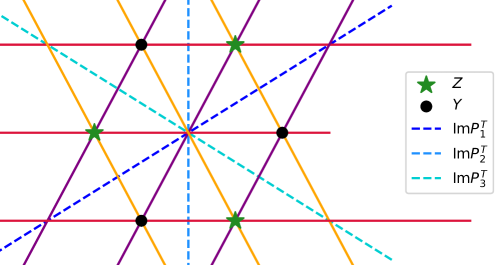
Figure 3: Illustration of a pathological super-critical case without unicity for specific projections $P_{i}$. In this case, $Y$ and $Z$ are distinct solutions with the same projections.

The points of $S$ are the points of the form $\displaystyle\bigcap\limits_{i=1}^{3}\left(z_{l_{i}}+\mathrm{Ker}P_{i}\right)$, or visually the intersection points of a yellow line, a red line and a purple line. We can see that the remaining vertices of the polygon constitute another valid measure $\gamma_{Y}$ whose push-forwards $P_{i}\#\gamma_{Y}$ are all the same as those of the original measure.

As mentioned in [6], for a fixed list of hyperplanes, there always exists two sets of points with the same projections on all of these hyperplanes. Theorem I.2 from [6] indicates that a necessary condition to ensure uniqueness in this case is $p>n$. In our Theorem 2, the points are fixed and uniqueness of the reconstruction holds almost surely when the $P_{i}$ follow assumption $\mathcal{A}{P}$ and as soon as $D>d$, whatever the number $n$ of points in the discrete measure.

2.4 Details on the critical case $\sum_{i}d_{i}=d$

In the theorem below, we show that the example in 2 is representative of the critical case.

Theorem 3 (Number of admissible points in the critical case).

Let $\gamma_{Z}$ be a fixed discrete probability measure. Assume that the matrices $P_{i}$ follow assumption $\mathcal{A}{P}$, and that $D:=\displaystyle\sum\limits_{i=1}^{p}d_{i}=d$. Then the cardinality of $S$ is exactly $n^{p}$, $\mathbb{P}$-a.s..

Proof.

We know that $S=\displaystyle\bigcup\limits_{\begin{subarray}{c}(l_{1},\cdots,l_{p})\in\llbracket 1,n\rrbracket^{p}\end{subarray}}\quad S_{\mathbf{l}}$ where $S_{\mathbf{l}}=\displaystyle\bigcap\limits_{i=1}^{p}\;\left(z_{l_{i}}+\mathrm{Ker}P_{i}\right)$. Following the proof of Theorem 2, in the case $D=d$, we see that assumption $\mathcal{A}{P}$ implies that $S_{\mathbf{l}}$ is almost surely a singleton $\{x_{\mathbf{l}}\}$. It follows that $S$ is almost surely the union of at most $n^{p}$ singletons. Let us show that if $\mathbf{l}\neq\mathbf{l^{\prime}}$ then $S_{\mathbf{l}}\cap S_{\mathbf{l^{\prime}}}=\varnothing$ a.s.. Indeed, if $x$ belongs to $S_{\mathbf{l}}\cap S_{\mathbf{l^{\prime}}}$ then $x$ is solution of a linear system of $2d$ equations:

$$\forall i\in\llbracket 1,p\rrbracket,\;\forall j\in\llbracket 1,d_{i}\rrbracket,\;\;\;\left\{\begin{array}[]{c}(u_{i}^{(j)})^{T}x=(u_{i}^{(j)})^{T}z_{l_{i}}\\ (u_{i}^{(j)})^{T}x=(u_{i}^{(j)})^{T}z_{l^{\prime}_{i}}\end{array}\right.,$$

which implies $\forall i\in\llbracket 1,p\rrbracket,\;\forall j\in\llbracket 1,d_{i}\rrbracket,\;\;\;l_{i}=l^{\prime}_{i},\;\text{ or }\;l_{i}\neq l_{i}^{\prime}\;\text{and}\;u_{l_{i}}^{(j)}\in(z_{l_{i}}-z_{l^{\prime}_{i}})^{\perp}$.

Now, under $\mathcal{A}{P}$, if $l_{i}\neq l_{i}^{\prime}$, then $\mathbb{P}(u_{l_{i}}^{(j)}\in(z_{l_{i}}-z_{l^{\prime}_{i}})^{\perp})=0$, and thus $\mathbf{l}=\mathbf{l}^{\prime}$ a.s..

∎

Let us clarify what the set of solutions $\mathcal{S}$ looks like in this critical case $D=d$. Let $\gamma$ be a solution of RP and denote $S=(x_{\mathbf{l}})_{\mathbf{l}\in\llbracket 1,n\rrbracket^{p}}$. By Theorem 3, $\gamma$ is of the form $\gamma=\displaystyle\sum\limits_{\mathbf{l}\in\llbracket 1,n\rrbracket^{p}}a_{\mathbf{l}}\delta_{x_{\mathbf{l}}}$. Now, since $\gamma$ is a solution, we have for $i\in\llbracket 1,p\rrbracket,\;P_{i}\#\gamma=P_{i}\#\gamma_{Z}$, thus$\displaystyle\sum\limits_{\mathbf{l}\in\llbracket 1,n\rrbracket^{p}}a_{\mathbf{l}}\delta_{P_{i}z_{l_{i}}}=\displaystyle\sum\limits_{k=1}^{n}b_{k}\delta_{P_{i}z_{k}}$. Since the $(P_{i}z_{l})_{l}$ are all distinct a.s., this entails for all $k\in\llbracket 1,n\rrbracket$: $\displaystyle\sum\limits_{\mathbf{l}_{-i}\in\llbracket 1,n\rrbracket^{p-1}}a_{l_{1},\cdots,l_{i-1},k,l_{i+1},\cdots,l_{p}}=b_{k}$, where $\mathbf{l}_{-i}$ indicates that we index this $(p-1)$-tuple on $\llbracket 1,n\rrbracket\setminus\{i\}$. We can re-write this condition as $a\in\Pi_{n}^{p}(b)$, the set of $n$-dimensional $p$-tensors on $\mathbb{R}_{+}$ ($\mathbb{R}_{+}^{n^{p}}$) with all $p$ marginals equal to $b$. Conversely, if $\gamma$ is of the form $\gamma=\displaystyle\sum\limits_{\mathbf{l}\in\llbracket 1,n\rrbracket^{p}}a_{\mathbf{l}}\delta_{x_{\mathbf{l}}}$ with $a\in\Pi_{n}^{p}(b)$, then we have by construction $\forall i\in\llbracket 1,p\rrbracket,\;P_{i}\#\gamma=P_{i}\#\gamma_{Z}$ and thus $\gamma$ is a solution.

In the particular case where $\gamma_{Z}$ is uniform, if we restrain $\gamma$ to be also a uniform measure, the problem in this critical case has a combinatorial amount of solutions. Without this restriction, the problem has an infinite amount of solutions, as is discussed in the particular case of 2.

3 Consequence for the empirical Sliced Wasserstein Distance

The Sliced Wasserstein distance between probability measures is frequently used in applied fields such as image processing or machine learning, as a more efficient alternative to the Wasserstein distance. It was introduced in [14] to generate barycenters between images of textures, and it is commonly used nowadays as a loss  [11, 5, 16] to train generative networks. This distance writes:

$$\forall\alpha,\beta\in\mathcal{P}_{2}(\mathbb{R}^{d}),\quad\mathrm{SW}^{2}(\alpha,\beta)=\int_{\theta\in\SS^{d}}{}\mathrm{W}_{2}^{2}(P_{\theta}\#\alpha,P_{\theta}\#\beta)\mathrm{d}\bbsigma(\theta),$$

where $\bbsigma$ is the uniform distribution over the unit sphere $\SS^{d}$ of $\mathbb{R}^{d}$, and $P_{\theta}$ denotes the linear projection on the line of direction $\theta$. In its empirical (Monte-Carlo) approximation, used for numerical applications, it becomes:

$$\forall\alpha,\beta\in\mathcal{P}_{2}(\mathbb{R}^{d}),\quad\widehat{\mathrm{SW}}_{p}^{2}(\alpha,\beta):=\cfrac{1}{p}\displaystyle\sum\limits_{i=1}^{p}\mathrm{W_{2}^{2}}(P_{\theta_{i}}\#\alpha,P_{\theta_{i}}\#\beta).$$ (3)

Since $\mathrm{W}_{2}$ is a distance on $\mathcal{P}_{2}(\mathbb{R}^{d})$ (the space of probability measures over $\mathbb{R}^{d}$ admitting a finite second-order moment), $\widehat{\mathrm{SW}}_{p}$ is non-negative, homogeneous and satisfies the triangle inequality. However, $\widehat{\mathrm{SW}}_{p}$ is only a pseudo-distance since it does not satisfy the separation property: whatever the $p$ directions chosen, it is always possible to find two different distributions $\alpha$ and $\beta$ such that $\widehat{\mathrm{SW}}_{p}(\alpha,\beta)=0$. Now, our previous reconstruction results show that when the $p$ directions are drawn from $\bbsigma$ and $\beta$ is a fixed discrete measure, then $\forall\alpha\in\mathcal{P}_{2}(\mathbb{R}^{d}),\;\widehat{\mathrm{SW}}_{p}^{2}(\alpha,\beta)~{}=~{}0~{}\Longrightarrow~{}\alpha~{}=~{}\beta$ almost surely provided that $p>d$. Indeed, $\widehat{\mathrm{SW}}_{p}(\alpha,\beta)=0$ if and only if $\alpha$ belongs to the set $\mathcal{S}$ (for $\gamma_{Z}=\beta$). On the contrary, when the number of projections is too small, the set of discrete measures at distance $0$ from a given one is infinite, as stated in the theorem below, and using $\widehat{\mathrm{SW}}_{p}$ in this setting as a loss between measures is unsound.

Theorem 4.

Let $\gamma_{Z}:=\displaystyle\sum\limits_{l=1}^{n}b_{l}\delta_{z_{l}}$, where the $(z_{l})$ are fixed and distinct. Assume $\theta_{1},\cdots,\theta_{p}\sim\bbsigma^{\otimes p}$.

• if $p\leq d$, there exists $\bbsigma$-a.s. an infinity of measures $\gamma\neq\gamma_{Z}\in\mathcal{P}_{2}(\mathbb{R}^{d})$ s.t. $\widehat{\mathrm{SW}}_{p}(\gamma,\gamma_{Z})=0$.

• if $p>d$, we have $\bbsigma$-almost surely $\{\gamma_{Z}\}=\underset{\gamma\in\mathcal{P}_{2}(\mathbb{R}^{d})}{\operatorname{argmin}}\;\widehat{\mathrm{SW}}_{p}(\gamma,\gamma_{Z})$.

In the limit case $p=d$, the distance can be grown by scaling the points of $\gamma_{Z}$ further away from the origin. In the case $p<d$, the supports of solution measures can be infinitely far from the support of $\gamma_{Z}$, as illusrated in 1.

4 Conclusion: Discussion on SW as a Loss in Machine Learning

In Sliced-Wasserstein-based Machine Learning, the question of global optima is paramount since in practice, one must default to a surrogate of $\mathrm{SW}$: be it through stochastic gradient descent (drawing a batch of $\theta_{i}$ at each iteration), or directly through the estimation $\widehat{\mathrm{SW}}_{p}$. To be precise, generative models such as [5] minimize $\theta\longmapsto\mathrm{SW}(T_{\theta}\#\mu_{0},\mu)$ - or a surrogate thereof - where $\mu_{0}$ is a low-dimensional input distribution (often chosen as realizations of Gaussian noise), where $\mu$ is the target distribution (the discrete dataset), and where $T_{\theta}$ is the model of parameters $\theta$. In this case, the dimension $d$ of the data, which for images can easily exceed one million, can be very large. Our results show that performing optimisation with less than $d$ projections is unsound, since it leads to solutions that can be arbitrarily far away from the true data distribution.

Furthermore, it is important to underline that having the guarantee that the global optima are the desired original measure is insufficient in practice. Indeed, the landscape $Y\longmapsto\widehat{\mathrm{SW}}_{p}(\mu_{Y},\mu_{Z})$ can present numerous local optima, which can limit the usefulness of SW as a loss function. For practical considerations, this study on global optima could be complemented by an analysis of the aforementioned landscape, which we leave for future work.

References

- [1] Nicolas Bonneel, Julien Rabin, Gabriel Peyré, and Hanspeter Pfister. Sliced and radon wasserstein barycenters of measures. Journal of Mathematical Imaging and Vision, 51(1):22–45, 2015.
- [2] Harald Cramér and Herman Wold. Some theorems on distribution functions. Journal of the London Mathematical Society, 1(4):290–294, 1936.
- [3] CM Cuadras. Probability distributions with given multivariate marginals and given dependence structure. Journal of multivariate analysis, 42(1):51–66, 1992.
- [4] Giorgio Dall’Aglio, Samuel Kotz, and Gabriella Salinetti. Advances in probability distributions with given marginals: beyond the copulas, volume 67. Springer Science & Business Media, 2012.
- [5] Ishan Deshpande, Ziyu Zhang, and Alexander G. Schwing. Generative modeling using the sliced wasserstein distance. In 2018 IEEE Conference on Computer Vision and Pattern Recognition, CVPR 2018, Salt Lake City, UT, USA, June 18-22, 2018, pages 3483–3491. Computer Vision Foundation / IEEE Computer Society, 2018.
- [6] Aingeru Fernandez-Bertolin, Philippe Jaming, and Karlheinz Grochenig. Determining point distributions from their projections. pages 164–168, 07 2017.
- [7] Richard J Gardner and Peter Gritzmann. Uniqueness and complexity in discrete tomography, 1999.
- [8] Nikita A Gladkov, Alexander V Kolesnikov, and Alexander P Zimin. On multistochastic monge–kantorovich problem, bitwise operations, and fractals. Calculus of Variations and Partial Differential Equations, 58:1–33, 2019.
- [9] A Heppes. On the determination of probability distributions of more dimensions by their projections. Acta Mathematica Hungarica, 7(3-4):403–410, 1956.
- [10] Harry Joe. Parametric families of multivariate distributions with given margins. Journal of multivariate analysis, 46(2):262–282, 1993.
- [11] Tero Karras, Timo Aila, Samuli Laine, and Jaakko Lehtinen. Progressive growing of GANs for improved quality, stability, and variation. 2018.
- [12] Nabil Kazi-Tani and Didier Rullière. On a construction of multivariate distributions given some multidimensional marginals. Advances in Applied Probability, 51(2):487–513, 2019.
- [13] Hans G Kellerer. Verteilungsfunktionen mit gegebenen marginalverteilungen. Zeitschrift für Wahrscheinlichkeitstheorie und verwandte Gebiete, 3:247–270, 1964.
- [14] Julien Rabin, Gabriel Peyré, Julie Delon, and Marc Bernot. Wasserstein barycenter and its application to texture mixing, 2012.
- [15] Alfréd Rényi. On projections of probability distributions. Acta Math. Acad. Sci. Hungar, 3(3):131–142, 1952.
- [16] J. Wu, Z. Huang, D. Acharya, W. Li, J. Thoma, D. Paudel, and L. Van Gool. Sliced wasserstein generative models. In 2019 IEEE/CVF Conference on Computer Vision and Pattern Recognition (CVPR), pages 3708–3717, Los Alamitos, CA, USA, jun 2019. IEEE Computer Society.