Rapidly time-varying reconfigurable intelligent surfaces for downlink multiuser transmissions

Abstract

Amplitude, phase, frequency, and polarization states of electromagnetic (EM) waves can be dynamically manipulated by means of artificially engineered planar materials, composed of sub-wavelength meta-atoms, which are typically referred to as metasurfaces. In wireless communications, metasurfaces can be configured to judiciously modify the EM propagation environment in such a way to achieve different network objectives in a digitally programmable way. In such a context, metasurfaces are typically referred to as reconfigurable intelligent surfaces (RISs). Until now, researchers in wireless communications have mainly focused their attention on slowly time-varying designs of RISs, where the spatial-phase gradient across the RIS is varied at the rate equal to the inverse of the channel coherence time. Additional degrees of freedom for controlling EM waves can be gained by applying a time modulation to the reflection response of RISs during the channel coherence time interval, thereby attaining rapidly time-varying RISs. In this paper, we develop a general framework where a downlink multiuser transmission over single-input single-output slow fading channels is assisted by a digitally controlled rapidly time-varying RIS. We show that reconfiguring the RIS at a rate greater than the inverse of the channel coherence time might be beneficial from a communication perspective depending on the considered network utility function and the available channel state information at the transmitter (CSIT). The conclusions of our analysis in terms of system design guidelines are as follows: (i) if the network utility function is the sum-rate time-averaged network capacity, without any constraint on fair resource allocation, and full CSIT is available, it is unnecessary to change the electronic properties of the RIS within the channel coherence time interval; (ii) if partial CSIT is assumed only, a rapidly time-varying randomized RIS allows to achieve a suitable balance between sum-rate time-averaged capacity and user fairness, especially for a sufficiently large number of users; (iii) regardless of the available amount of CSIT, the design of rapid temporal variations across the RIS is instrumental for developing scheduling algorithms aimed at maximizing the network capacity subject to fairness constraints.

I Introduction

Since the birth of radio communications in the early $1900$s, engineers, mathematicians, and physicists have dealt with the uncontrollable nature of propagation environments. Reconfigurable intelligent surfaces (RISs) are emerging as an innovative technology for the electromagnetic (EM) wave manipulation, signal modulation, and smart radio environment reconfiguration in wireless communications systems [1, 2, 3, 4, 5, 6]. An RIS is a metasurface composed of uniform or non-uniform sub-wavelength metal/dielectric structures, referred to as meta-atoms (or unit cells), which interact with the incident EM fields, whose working frequency can vary from sub-$6$ GHz to THz. Such meta-atoms can be independently controlled via software to switch among different reflection amplitude and phase responses that collectively shape the wavefront of the impinging wave [7, 8], without the need of bulky phase shifters. Thanks to their ultra-thin profile, square-law array gain, low-power consumption, low noise, and easy fabrication and deployment, RISs yield more freedom and flexibility to create different reflecting patterns for incident waves from diverse directions [9, 10, 11, 12, 13], compared to conventional phased antenna arrays. RISs can be realized by embedding into meta-atoms tunable varactor diodes, switchable positive-intrinsic-negative (PIN) diodes, field effect transistors, or micro-electromechanical system switches, which collectively form an inhomogeneous surface with specific phase profiles [14, 15, 16, 17, 18].

In wireless communications, the channel response may change with time. The channel coherence time is a measure of the expected time duration over which the response of the channel is essentially invariant and it is related to the bandwidth of the Doppler spectrum. Due to the time-varying nature of wireless channels, the reflection coefficient of the meta-atoms has to be varied in both space and time domains, thus leading to the so-called space-time metasurfaces in the EM literature [19, 20, 21, 22, 23, 24, 25, 26, 27, 28, 29, 30, 31, 32, 33, 34, 35]. In slowly time-varying design techniques, the rate at which the reflecting coefficients of the meta-atoms are updated is equal to the inverse of the channel coherence time. For each channel coherence time interval, anomalous reflection/refraction (for beam steering) and reflective/transmissive focusing (for high directivity) are obtained by spatially varying the state of meta-atoms at different positions on the RIS. In this paper, we instead consider rapidly time-varying design techniques: in this case, besides constructing the spatially varying phase profile, the phase responses of the meta-atoms are modulated in time during the channel coherence time interval, by assuming that the time-modulation speed is much smaller than the frequency of the incident EM signal. Rapidly time-varying RISs offer additional degrees of freedom for manipulating signals, such as, e.g., nonlinear harmonic manipulations [32] and spread-spectrum camouflaging [33].

Relying on the feasibility of engineering the meta-atoms on the metasurface, a plethora of papers has been published where the wireless channel is programmed by optimizing on-the-fly the response of built-in RISs to achieve different system objectives, such as capacity gains [36, 37, 38, 39, 40, 41, 42], coverage extension [44, 43], energy efficiency [45, 46], maximization of minimum signal-to-noise ratio (SNR) [47], joint maximization of rate and energy efficiency [48], quality of services (QoS) targets under imperfect channel state information (CSI) [49], super resolution CSI estimation [50], and high level of localization accuracy [51]. When the control of the RIS is performed by the transmitter, the RIS is also equipped with a smart controller that communicates with the transmitter via a separate wireless link for coordinating transmission and exchanging information on the phase shifts of all reflecting elements in real time. In this scenario, CSI at the transmitter (CSIT) is required to derive the optimal response of the RIS.

To the best of our knowledge, almost all the studies within the wireless communications community consider only slowly time-varying RISs. Notable exceptions are represented by [52] and [53]. Along the same lines of [21], only point-to-point communication (i.e., the scenario of a single transmitter and a single receiver) has been considered in [52]. In [53], the modulation in time of the reflection response of the RIS is used to transmit information over a full-duplex point-to-point link. Nevertheless, the use of rapidly time-varying RISs specifically subordinated to the interest of a network of many users (i.e., RISs do not transmit their own information) remains an unexplored issue and their benefits in multiuser communications have not been studied yet.

I-A Contributions

We focus on a single-input single-output downlink of a wireless communication multiuser system operating over a slow fading channel with coherence time $T_{\text{c}}$, which is assumed to be much longer than the symbol period of the transmit digital modulator. We assume a delay-tolerant scenario, where the user rates can be adapted according to their instantaneous channel conditions. The scheduler function in the medium-access-control sublayer of the transmitter consists of dividing each channel coherence time interval in time slots and introducing a scheme for resource assignment among the users. The downlink transmission is assisted by a digital rapidly time-varying RIS, whose reflection response is fixed during each time slot, but it can be digitally varied in both time and space domains from one time slot to another in a controlled manner. Besides channel conditions, the total system performance and the data rate of each user are affected by the scheme used for scheduling and the states of the reflection coefficients of the RIS meta-atoms. The contributions of this study are summarized as follows.

1. We prove that maximization of the sum-rate time-averaged capacity, with respect to transmit powers allocated at the users and reflection coefficients of the meta-atoms, can be achieved by a slowly time-varying RIS in the case of full CSIT. In this case, the reflection coefficients can be optimized with a manageable computational complexity by resorting to the block-coordinate descent (or Gauss-Seidel) method [54], which accounts for discrete variations of the reflection response of the RIS.

2. The scheduling deriving by the maximization of the sum-rate time-averaged capacity with a slowly time-varying RIS would result in a very unfair sharing of the channel resource, by letting only the user with the best channel condition to transmit during each channel coherence time interval. Moreover, in many applications, it is not reasonable to assume that full CSIT can be made available. To partially overcome such shortcomings, we propose to use a rapidly time-varying randomized RIS where the reflection coefficients of the meta-atoms are randomly varied from one time slot to another in both space and time. This induces random fluctuations in the overall channel seen by each user even if the physical channel has no fluctuations over a time interval of duration $T_{\text{c}}$. In this case, maximization of the sum-rate time-averaged capacity with respect to transmit powers allocated at the users requires only partial CSIT and more than one user may be scheduled during each channel coherence time interval.

3. To ensure a proportionally fair allocation of channel resource [55], we show that, when the aim is to maximize the sum of logarithmic exponentially weighted moving average user rates, a rapidly time-varying RIS is the natural solution in the case of both full and partial CSIT.

I-B Notations

Upper- and lower-case bold letters denote matrices and vectors; the superscripts $*$, T and H denote the conjugate, the transpose, and the Hermitian (conjugate transpose) of a matrix; $[x]^{+}$ stands for $\max\{x,0\}$; $\mathbb{C}$, $\mathbb{R}$ and $\mathbb{Z}$ are the fields of complex, real and integer numbers; $\mathbb{C}^{n}$ $[\mathbb{R}^{n}]$ denotes the vector-space of all $n$-column vectors with complex [real] coordinates; similarly, $\mathbb{C}^{n\times m}$ $[\mathbb{R}^{n\times m}]$ denotes the vector-space of all the $n\times m$ matrices with complex [real] elements; $j\triangleq\sqrt{-1}$ denotes the imaginary unit; $\Re\{x\}$ is the real part of $x\in\mathbb{C}$; $\ast$ denotes the (linear) convolution operator; $\Pi(t)$ is the basic rectangular window, i.e., $\Pi(t)=1$ for $|t|\leq 1/2$ and zero otherwise; $\lfloor x\rfloor$ rounds $x\in\mathbb{R}$ to the nearest integer less than or equal to that element; $\otimes$ is the Kronecker product; $\mathbf{0}_{n}$, ${\mathbf{O}}_{n\times m}$ and ${\mathbf{I}}_{n}$ denote the $n$-column zero vector, the $n\times m$ zero matrix and the $n\times n$ identity matrix; matrix $\mathbf{A}={\text{diag}}(a_{0},a_{1},\ldots,a_{n-1})\in\mathbb{C}^{n\times n}$ is diagonal; $\{\mathbf{A}\}_{i,\ell}$ indicates the $(i,\ell)$th element of $\mathbf{A}\in\mathbb{C}^{n\times m}$, with $i\in\{1,2,\ldots,n\}$ and $\ell\in\{1,2,\ldots,m\}$; $\|\mathbf{a}\|$ denotes the Frobenius norm of $\mathbf{a}\in\mathbb{C}^{n}$; ${\mathbb{E}}[\cdot]$ denotes ensemble averaging; ${\mathbf{x}}\sim{\cal CN}(\boldsymbol{\mu},{\mathbf{C}})$ is a circularly symmetric complex Gaussian vector ${\mathbf{x}}\in\mathbb{C}^{n}$ with mean $\boldsymbol{\mu}\in\mathbb{C}^{n}$ and covariance ${\mathbf{C}}\in\mathbb{C}^{n\times n}$.

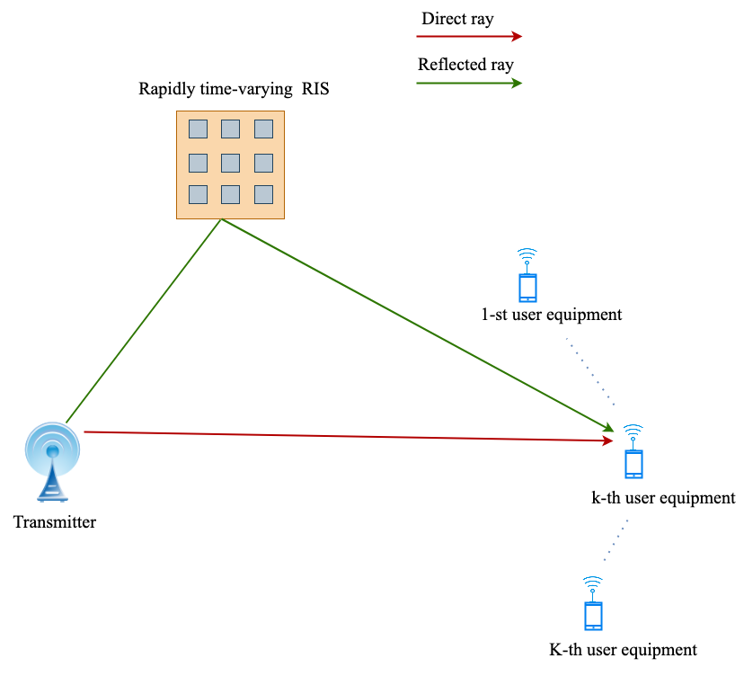
Figure 1: A pictorial view of a downlink transmission in a multiuser system assisted by a rapidly time-varying RIS. In the figure, the direct and reflected rays of the generic $k$-th user are depicted only, with $k\in\{1,2,\ldots,K\}$.

II Downlink with rapidly time-varying RIS

With reference to Fig. 1, we consider a wireless system including a single-antenna transmitter, whose aim is to transfer information in downlink to $K>1$ single-antenna user equipments (UEs). The transmission is assisted by a digitally programmable RIS working in reflection mode, which is installed on the face of a surrounding high-rise building, indoor walls, or roadside billboards. The RIS is made of $Q=Q_{x}\times Q_{y}$ spatial meta-atoms, which are positioned along a rectangular grid having $Q_{x}$ and $Q_{y}$ elements on the $x$ and $y$ axes, respectively. The meta-atoms are independently controlled to switch among different EM responses that collectively shape the spatial and spectral characteristics of the illuminating wave in a time-varying fashion [19, 20, 21, 22, 23, 24, 25, 26, 27, 28, 29, 30]. The functionality of such a metasurface is determined by the instantaneous digital reflection response of each meta-atom, which can be dynamically controlled by digital logic devices [7, 8]. We consider a transmission system with baud rate $1/T_{\text{s}}$. Throughout the paper, we assume that the communication bandwidth $W\propto 1/T_{\text{s}}$ is much smaller than the carrier frequency $f_{0}$ (narrowband assumption), i.e., $f_{0}\,T_{\text{s}}\gg 1$. Narrowband frequency-flat channels are considered with coherence time $T_{\text{c}}$ spanning $L_{\text{c}}$ symbol intervals, i.e., $T_{\text{c}}=L_{\text{c}}\,T_{\text{s}}$. These channels are modeled by a single-tap filter, as most of the multipaths arrive during one symbol time, which is approximately constant within frame intervals of length $T_{\text{c}}$, but is allowed to independently change from one coherence period to another (block fading model). Each channel tap coefficient is formed by the superposition of a large number of micro-scattering components (e.g., due to rough surfaces) having (approximately) the same delay. By virtue of the central limit theorem, it is customary to model the superposition of such many small effects as Gaussian [58].

The signal received by each user consists of two components (see Fig. 1): the direct ray, which corresponds to the signal propagating from the transmitter to the $k$-th UE with propagation delay $\tau_{0,k}$, and a reflected ray, which is the signal reflected off the RIS with (overall) propagation delay $\tau_{1,k}$. The delay spread $\Delta_{k}\triangleq\tau_{1,k}-\tau_{0,k}$ of the composite $k$-th channel (i.e., direct and reflected rays) equals the difference between the delay of the direct ray and that of the reflected one. We assume that the transmitted signal is also narrowband relative to the delay spread, i.e., $\Delta_{k}\ll T_{\text{s}}$, such that the effects of $\tau_{0,k}$ and $\tau_{1,k}$ can be ignored at the $k$-th UE.

II-A Signal emitted by the transmitter

Each channel coherence time interval is divided into $M$ time slots of duration $T_{\text{r}}\triangleq T_{\text{c}}/M$. Each slot spans $P$ symbols intervals, i.e., $T_{\text{r}}=P\,T_{\text{s}}$. Consequently, it results that $L_{\text{c}}=M\,P$. Let $s_{k}(n)$ be the information-bearing symbol intended for the $k$-th user within the $n$-th symbol interval, for $k\in\{1,2,\ldots,K\}$ and $n\in\mathbb{Z}$. The transmitted symbols $\{s_{k}(n)\}_{n\in\mathbb{Z}}$ are modeled as mutually independent sequences of zero-mean unit-variance independent and identically distributed (i.i.d.) complex circular random variables. For each $k\in\{1,2,\ldots,K\}$, the data stream $\{s_{k}(n)\}_{n\in\mathbb{Z}}$ of the $k$-th user at rate $1/T_{\text{s}}$ is converted at the transmitter side into $M$ parallel substreams $s^{(m)}_{k}(p)\triangleq s_{k}(p\,P+m)$, for $p\in\{0,1,\ldots,P-1\}$ and $m\in\{0,1,\ldots,M-1\}$. Such substreams are superposed as follows

$$s^{(m)}(p)=\sum_{k=1}^{K}\sqrt{\mathcal{P}_{k}^{(m)}}\,s^{(m)}_{k}(p)$$ (1)

where $\mathcal{P}_{k}^{(m)}$ is the transmit power allocated to the $k$-th user in the $m$-th slot, subject to the time-averaged sum-power constraint $\frac{1}{M}\sum_{k=1}^{K}\sum_{m=0}^{M-1}\mathcal{P}_{k}^{(m)}\leq\mathcal{P}_{\text{TX}}$, where $\mathcal{P}_{\text{TX}}>0$ denotes the (fixed) maximum allowed transmit power. With reference to a generic coherence interval, the continuous-time baseband signal emitted by the transmitter reads as

$$x(t)=\sum_{m=0}^{M-1}\sum_{p=0}^{P-1}s^{(m)}(p)\,\psi\left(t-p\,T_{\text{s}}-m\,T_{\text{r}}\right)$$ (2)

where $\psi(t)$ is the unit-energy square-root Nyquist pulse-shaping filter [58]. In this case, the communication bandwidth is $W=(1+\varrho_{\text{s}})/T_{\text{s}}$, with $0\leq\varrho_{\text{s}}\leq 1$ being the rolloff factor.

II-B Rapidly time-varying RIS

The RISs widely studied in existing works [7, 8, 9, 10, 11, 12, 13, 14, 15, 16, 17, 18, 19, 20, 21, 22, 23, 24, 25, 26, 27, 28, 29, 30] consume minimal power, which can be as low as a few $\mu$W per meta-atom, and the introduced thermal noise is also negligible. By assuming that the reflection-response of the RIS is frequency flat, i.e., it is constant over the whole signal bandwidth $W$, the far-field baseband signal reflected by a rapidly time-varying RIS reads as

$${\mathbf{z}}(t)={\mathbf{R}}(t)\,{\mathbf{g}}\,x(t)$$ (3)

with ${\mathbf{R}}(t)\triangleq{\text{diag}}\left[\gamma_{1}(t),\gamma_{2}(t),\ldots,\gamma_{Q}(t)\right]$, where according to the time-switched array theory [23, 22], the complex parameter $\gamma_{q}(t)$ is the time-modulated reflection coefficient of the $q$-th meta-atom, $\forall q\in\{1,2,\ldots,Q\}$, whereas ${\mathbf{g}}\in\mathbb{C}^{Q}$ denotes the low-pass equivalent channel response between the transmitter and the RIS within the considered channel coherence time. RISs have the capability of controlling the amplitude, phase, and polarization of incident EM waves [59]. Design methods of programmable RISs have been proposed in [60, 61, 62] where the reflection magnitude and phase can be independently controlled. We focus on an RIS with phase-only modulation, by deferring the case of RISs with amplitude-phase modulated elements to future work.

If ${\mathbf{R}}(t)$ does not vary during each channel coherence time interval, the effect of the RIS consists of multiplying the impinging signal ${\mathbf{g}}\,x(t)$ by a constant matrix ${\mathbf{R}}(t)\equiv{\mathbf{R}}$, i.e., slowly time-varying RIS, which is the configuration considered in previous works [1, 2, 3, 4, 5, 6, 36, 37, 38, 39, 40, 41, 42, 44, 43, 45, 46, 47, 48, 49, 50, 51]: in this case, each UE sees a time-invariant overall channel (see also Subsection II-D). In this paper, relying on the results of recent experimental studies [19, 20, 21, 22, 23, 24, 25, 26, 27, 28, 29, 30, 34, 35], we consider the case where ${\mathbf{R}}(t)$ is time-varying over the channel coherence time interval. In its simplest form, the reflection coefficient of the generic $q$-th meta-atom is subject to a linear modulation as

$$\gamma_{q}(t)=\sum_{m=0}^{M-1}\gamma_{q}^{(m)}\,\phi(t-m\,T_{\text{r}})$$ (4)

where $\phi(t)=\Pi\left(\frac{t-T_{\text{r}}/2}{T_{\text{r}}}\right)$ is a pulse-shaping filter of duration $T_{\text{r}}$, the complex coefficients $\gamma_{q}^{(0)},\gamma_{q}^{(1)},\ldots,\gamma_{q}^{(M-1)}$ are at the designer’s disposal. For an $b$-bit digital meta-atom with phase-only modulation capability, each coefficient $\gamma_{q}^{(m)}$ assumes values in the set $\mathcal{R}\triangleq\{R_{0},R_{1},\ldots,R_{2^{b}-1}\}$ of cardinality $2^{b}$, with elements $R_{\ell}\triangleq\exp(j\frac{2\pi}{2^{b}}\ell)$, for $\ell\in\{0,1,\ldots,2^{b}-1\}$. By considering the balance between the system cost, design complexity, and overall performance, it has been found that $b$-bit meta-atoms are suitable for RIS implementation [63], for small-to-moderate values of $b$.

TABLE I: Summary of the main system parameters and the time-scale of change of the key physical quantities.

Key parameters and time-scales	Symbols	Values for an exemplifying scenario
Carrier frequency	$f_{0}$	$1.5$ GHz
Communication bandwidth	$W$	$5$ MHz
Rolloff factor	$\varrho_{\text{s}}$	$0.25$
Symbol period	$T_{\text{s}}=(1+\varrho_{\text{s}})/W$	$250$ ns
Channel coherence time	$T_{\text{c}}$	$50$ ms
Number of symbols per channel coherence interval	$L_{\text{c}}=\lfloor T_{\text{c}}/T_{\text{s}}\rfloor$	$200,000$
Switching frequencies of meta-atoms	$f_{\text{r}}=1/T_{\text{r}}$	$50$ kHz
Number of slots per channel coherence interval	$M=\lfloor T_{\text{c}}/T_{\text{r}}\rfloor$	$2500$
Number of symbols per slot	$P=\lfloor T_{\text{r}}/T_{\text{s}}\rfloor$	$80$

According to [19, 20, 21, 22, 23, 24, 25, 26, 27, 28, 29, 30, 34, 35], eq. (3) is approximately valid when the reflection coefficients vary at a very slow pace compared to the carrier frequency of the impinging signal, i.e., the switching frequency $f_{\text{r}}\triangleq 1/T_{\text{r}}$ is much smaller than $f_{0}$ or, equivalently, $f_{0}\,T_{\text{r}}\gg 1$. This operative condition is surely satisfied in the narrowband regime since $T_{\text{r}}>T_{\text{s}}$ by assumption. The main system parameters and the time-scale of change of key quantities are summarized in the first two columns of Table I, whereas their values are reported in the third column for an exemplifying scenario of practical interest. In particular, the values of the carrier frequency $f_{0}$ and the communication bandwidth $W$ are consistent with Frequency Range 1 (FR1) of 5G New Radio (NR) [64]. The value of the channel coherence time is typical of a pedestrian scenario. In current implementations [19, 20, 21, 22, 23, 24, 25, 26, 27, 28, 29, 30, 35], the switching frequencies of the meta-atoms can reach tens of MHz. Larger values of $f_{\text{r}}$ can be achieved by exploiting faster switching mechanisms based on innovative materials, such as graphene or vanadium dioxide [65]. However, the time variation induced by the RIS should be slow enough and should happen at a time scale allowing the reflection response ${\mathbf{R}}(t)$ to be unaffected by the receiving filter at the UEs (see Subsection II-C). Further, the variation should be slow enough to ensure that CSI is reliably acquired (see Subsection II-F).

II-C Signal received by each user

We customarily assume that each UE uses standard timing synchronization with respect to its direct link. To decode the data signal, each UE performs matched filtering with respect to the symbol pulse $\psi(t)$. After matched filtering and sampling with rate $1/T_{\text{s}}$ at time instants $t_{p}^{(m)}\triangleq p\,T_{\text{s}}+m\,T_{\text{r}}$, with $p\in\{0,1,\ldots,P-1\}$ and $m\in\{0,1,\ldots,M-1\}$, the discrete-time baseband signal received at the $k$-th user reads as

$$r_{k}^{(m)}(p)=\underbrace{h_{k}^{*}\,x(t)\ast\psi(-t)}_{\text{Direct link}}\Big{|}_{t=t_{p}^{(m)}}\\ +\underbrace{{\mathbf{f}}_{k}^{\text{H}}\,{\mathbf{z}}(t)\ast\psi(-t)}_{\text{Reflection link}}\Big{|}_{t=t_{p}^{(m)}}+v_{k}^{(m)}(p)$$ (5)

for $k\in\{1,2,\ldots,K\}$, where $h_{k}\in\mathbb{C}$ models the low-pass equivalent channel response from the transmitter to user $k$, the vector ${\mathbf{f}}_{k}\in\mathbb{C}^{Q}$ denotes the low-pass equivalent channel response from the RIS to the $k$-th user, and $v_{k}^{(m)}(p)\sim{\cal CN}(0,1)$ is the noise sample at the output of the matched filter, with $v_{k_{1}}^{(m_{1})}(p_{1})$ statistically independent of $v_{k_{2}}^{(m_{2})}(p_{2})$, for $k_{1}\neq k_{2}$, $p_{1}\neq p_{2}$, and $m_{1}\neq m_{2}$. Without loss of generality, we have assumed that the noise has unit variance. Hence, the parameter $\mathcal{P}_{\text{TX}}$ in Subsection II-A takes on the meaning of total transmit signal-to-noise ratio (SNR).

By substituting (2)-(3) in (5), and accounting for (4), the block ${\mathbf{r}}_{k}^{(m)}\triangleq[r_{k}^{(m)}(0),r_{k}^{(m)}(1),\ldots,r_{k}^{(m)}(P-1)]^{\text{T}}\in\mathbb{C}^{P}$ received by the $k$-th user within the $m$-th slot is given by

$${\mathbf{r}}_{k}^{(m)}=[c_{k}^{(m)}]^{*}\left[\sum_{u=1}^{K}\,\sqrt{\mathcal{P}_{u}^{(m)}}\,{\mathbf{s}}_{u}^{(m)}\right]+{\mathbf{v}}_{k}^{(m)}$$ (6)

where the overall channel gain seen by the $k$-th UE during the $m$-th slot can be written as

$$c_{k}^{(m)}\triangleq h_{k}+{\mathbf{g}}^{\text{H}}\,[{\mathbf{\Gamma}}^{(m)}]^{*}\,{\mathbf{f}}_{k}\in\mathbb{C}\>,\quad\text{for $k\in\{1,2,\ldots,K\}$}$$ (7)

with

$${\mathbf{\Gamma}}^{(m)} \triangleq{\text{diag}}\left[\gamma_{1}^{(m)},\gamma_{2}^{(m)},\ldots,\gamma_{Q}^{(m)}\right]$$ (8)

$${\mathbf{s}}_{k}^{(m)} \triangleq[s_{k}^{(m)}(0),s_{k}^{(m)}(1),\ldots,s_{k}^{(m)}(P-1)]^{\text{T}}\in\mathbb{C}^{P}$$ (9)

$${\mathbf{v}}_{k}^{(m)} \triangleq[v_{k}^{(m)}(0),v_{k}^{(m)}(1),\ldots,v_{k}^{(m)}(P-1)]^{\text{T}}\in\mathbb{C}^{P}\>.$$ (10)

In eq. (6), we have used $[{\mathbf{R}}(t)\,{\mathbf{g}}\,x(t)]\ast\phi(-t)\approx{\mathbf{R}}(t)\,{\mathbf{g}}\,[x(t)\ast\phi(-t)]$, which holds if ${\mathbf{R}}(t)$ varies at a very slow pace compared to the effective duration of $\phi(t)$, i.e., $f_{\text{r}}\ll 1/T_{\text{s}}$ or, equivalently, $P\gg 1$. In many applications, the channel coherence time is of the order of hundreds to thousands symbols, and therefore sufficiently large values of $P$ can be chosen in these operative scenarios (see Table I for instance).

A key observation is now in order. The received signal (6) shows that, even though the channels $h_{k}$, ${\mathbf{g}}$, and ${\mathbf{f}}_{k}$ are time invariant over each coherence interval spanning $L_{\text{c}}$ consecutive symbol periods, the overall channel (7) seen by each user varies in time on a slot-by-slot basis. The rate of variation of $c_{k}^{(m)}$ in time is dictated by $M$, as well as the diagonal matrices ${\mathbf{\Gamma}}^{(0)},{\mathbf{\Gamma}}^{(1)},\ldots,{\mathbf{\Gamma}}^{(M-1)}$, which can be suitably controlled to dynamically schedule resources among the users and, thus, they are design parameters of the system. Strictly speaking, the overall effect of the rapidly time-varying RIS is to increase the rate and dynamic range of channel fluctuations.

II-D The conventional case of a slowly time-varying RIS

In many recent works [1, 2, 3, 4, 5, 6, 36, 37, 38, 39, 40, 41, 42, 44, 43, 45, 46, 47, 48, 49, 50, 51], the RIS does not introduce time variability during the transmission of an information-bearing symbol block, i.e., it is slowly time-varying. This can be regarded as a particular case of our general model, where $M=1$ and $T_{\text{r}}=T_{\text{c}}$ (see Fig. 2). In this special case, one has $\gamma_{q}(t)=\gamma_{q}^{(0)}$, for $q\in\{1,2,\ldots,Q\}$. Therefore, if the reflection process of the RIS is time invariant over each channel coherence time interval, that is, ${\mathbf{\Gamma}}^{(0)}={\mathbf{\Gamma}}^{(1)}=\cdots={\mathbf{\Gamma}}^{(M-1)}={\text{diag}}[\gamma_{1}^{(0)},\gamma_{2}^{(0)},\ldots,\gamma_{Q}^{(0)}]$, the overall channel vector (7) from the transmitter to each user becomes constant over each channel coherence time interval.

II-E Assumptions regarding the channels

It is common to model the channels between the transmitter and the meta-atoms of the RIS by assuming that the received wavefront is planar (see, e.g., [66]). In this case, the transmitter-to-RIS channel vector ${\mathbf{g}}$ can be modeled as

$${\mathbf{g}}=\sigma_{g}\left(\sqrt{\frac{\kappa}{\kappa+1}}+\sqrt{\frac{1}{\kappa+1}}\,g_{\text{DIF}}\right){\mathbf{a}}_{\text{RIS}}$$ (11)

where the first summand represents the (deterministic) line-of-sight (LoS) component, whereas the second one is the (random) diffuse (i.e., non-LoS) component, with $g_{\text{DIF}}\sim{\cal CN}(0,1)$. The variance $\sigma_{g}^{2}$ describes the large-scale geometric pathloss and $\kappa\geq 0$ is the Ricean factor. It is worthwhile to note that $\kappa=0$ yields Rayleigh fading, Rician fading is obtained when $\kappa>0$, and, in the limiting case $\kappa\to+\infty$, there is only the LoS channel component. The spatial signature ${\mathbf{a}}_{\text{RIS}}$ of the RIS in (11) is given by

$${\mathbf{a}}_{\text{RIS}}\triangleq\left[1,e^{j\frac{2\pi}{\lambda_{0}}d_{\text{RIS}}u_{x}},\ldots,e^{j\frac{2\pi}{\lambda_{0}}(Q_{x}-1)d_{\text{RIS}}u_{x}}\right]^{\text{T}}\\ \otimes\left[1,e^{j\frac{2\pi}{\lambda_{0}}d_{\text{RIS}}u_{y}},\ldots,e^{j\frac{2\pi}{\lambda_{0}}(Q_{y}-1)d_{\text{RIS}}u_{y}}\right]^{\text{T}}\in\mathbb{C}^{Q}$$ (12)

where $\lambda_{0}=c/f_{0}$ is the wavelength, with $c$ being the speed of light in the medium, $d_{\text{RIS}}$ is the inter-element spacing at the RIS, $\theta_{\text{RIS}}\in[0,2\pi)$ and $\phi_{\text{RIS}}\in[-\pi/2,\pi/2)$ identify the azimuth and elevation angles, respectively, whose directional cosines are $u_{x}\triangleq\sin\theta_{\text{RIS}}\,\cos\phi_{\text{RIS}}$ and $u_{y}\triangleq\sin\theta_{\text{RIS}}\,\sin\phi_{\text{RIS}}$. It should be noted that ${\mathbb{E}}[\|{\mathbf{g}}\|^{2}]=\sigma_{g}^{2}\,Q$.

The random channels $h_{k}$ and ${\mathbf{f}}_{k}$ are modeled as $h_{k}\sim{\cal CN}(0,\sigma_{h_{k}}^{2})$ and ${\mathbf{f}}_{k}\sim{\cal CN}({\mathbf{0}}_{Q},\sigma_{f_{k}}^{2}\,{\mathbf{I}}_{Q})$, with $g_{\text{DIF}}$, $h_{k}$, and ${\mathbf{f}}_{k}$ mutually independent, for each $k\in\{1,2,\ldots,K\}$. The parameters $\sigma_{h_{k}}^{2}$ and $\sigma_{f_{k}}^{2}$ are the large-scale geometric path losses of the link seen by the $k$-th user with respect to the transmitter and the RIS, respectively. The triplet $(g_{\text{DIF}},h_{k},{\mathbf{f}}_{k})$ is independent of the noise vectors ${\mathbf{v}}_{k}^{(m)}$, $\forall k\in\{1,2,\ldots,K\}$ and $\forall m\in\{0,1,\ldots,M-1\}$.

II-F High-level overview of the CSI acquisition process

In the sequel, we assume that, for each $k\in\{1,2,\ldots,K\}$, the $k$-th UE has perfect knowledge of its channel gain $c_{k}^{(m)}$, $\forall m\in\{0,1,\ldots,M-1\}$, referred to as CSI at the receiver (CSIR), which can be estimated through standard training algorithms, by using $N_{\text{down-full}}$ downlink pilot symbols repeated at the beginning of each slot. In this case, if the power spent by the transmitter for pilot symbol transmission is significantly greater than the noise variance, a single downlink pilot per slot (i.e., $N_{\text{down-full}}=1$) is sufficient to ensure that the channel estimation error is quite small [67]. On the other hand, we consider two different amount of CSIT:

1. In the case of full CSIT, the transmitter has perfect knowledge of all the relevant channel parameters $h_{k}$ and ${\mathbf{f}}_{k}$, $\forall k\in\{1,2,\ldots,K\}$, and ${\mathbf{g}}$.

2. In the case of partial CSIT, $\forall m\in\{0,1,\ldots,M-1\}$, the transmitter knows only the user index for which $|c_{k}^{(m)}|$ is maximized.

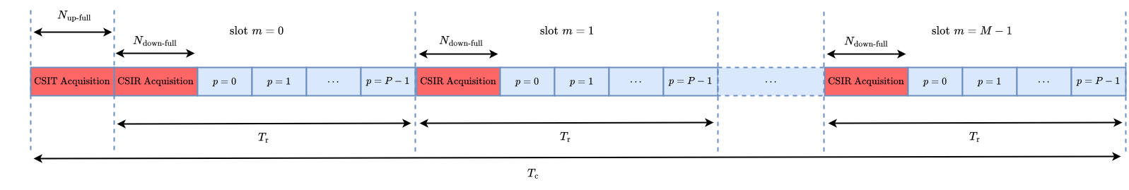
Figure 2: According to a TDD protocol, acquisition of full CSIT requires an uplink training phase at the beginning of each channel coherence time interval, in addition to downlink training phases for CSIR acquisition.

For acquisition of full CSIT, a viable strategy consists of resorting to a time-division duplexing (TDD) protocol. In this case, where channel reciprocity can be exploited, acquisition of full CSIT additionally requires a non-trivial uplink training session of $N_{\text{up-full}}$ pilot symbols at the beginning of each channel coherence time (see Fig. 2), which might be unrealistic in many scenarios of practical interest, especially for large values of $K$ and $Q$. Indeed, the CSIT estimation process requires $N_{\text{up-full}}\geq K(Q+1)$ pilot symbols [68].

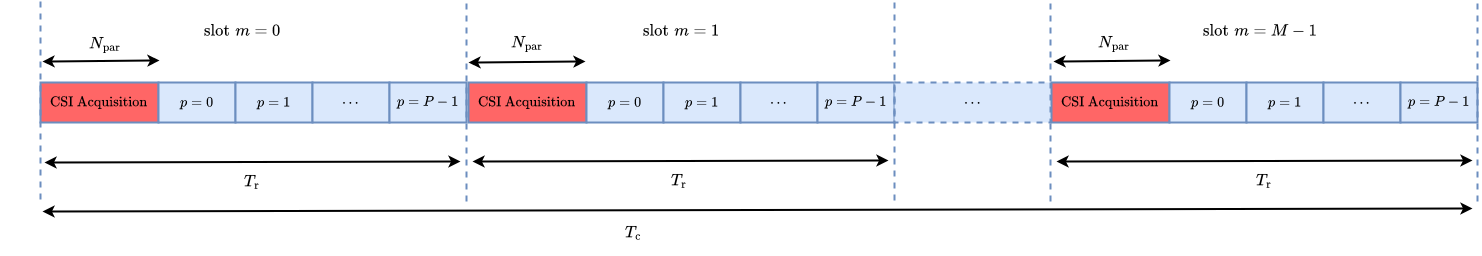
Figure 3: Acquisition of partial CSIT can be performed in a centralized or decentralized manner by providing at the beginning of each slot an initial phase devoted to both CSIR acquisition and discovery of the UE with the strongest path for downlink information transmission.

On the other hand, partial CSIT involves only the discovery of the UE having the “best” end-to-end path, which can be identified in a centralized or decentralized fashion. In the centralized case, each UE estimates its own channel coefficient $c_{k}^{(m)}$, through, say, a common downlink pilot and, then, feeds back the (quantized version of) instantaneous channel quality $|c_{k}^{(m)}|$ to the transmitter. In such a centralized scenario, the duration $N_{\text{par}}$ (in symbol intervals) of the CSI acquisition phase in Fig. 3 also depends on the delay in feeding $|c_{k}^{(m)}|$ back. If feedback control channels from each UE to the transmitter are not available, a decentralized CSI acquisition scheme can be implemented [70], according to which, after receiving a downlink training packet, each UE will start its own timer with an initial value that is inversely proportional to a local estimate of channel quality $|c_{k}^{(m)}|$. The timer of the UE with the strongest end-to-end channel will expire first and such an UE will transmit an uplink flag packet to the transmitter, communicating its identification number. In this decentralized scenario, the amount of overhead $N_{\text{par}}$ involved in selecting the best UE also depends on the statistics of the wireless channel (see [70] for a probabilistic analysis).

Since the capacity results reported in this paper are valid only when the required CSI is perfectly known at the transmitter and at the UEs, we do not account for channel estimation imperfections hereinafter, by deferring CSI estimation issues to a future work.

III Sum-rate time-averaged capacity: full CSIT

In this section, we assume full CSIT (see Subsection II-F). The achievable data rate transmitted to the $k$-th UE is affected by the interference from the signals intended for the other users $u\neq k\in\{1,2,\ldots,K\}$ on the same slot. Assuming that the transmitter encodes the information for each user using an i.i.d. Gaussian code, the time-averaged rate of user $k$ can be written as

$$\overline{\mathcal{R}}_{k}=\frac{1}{M}\sum_{m=0}^{M-1}\log_{2}\left[1+\text{SINR}_{k}^{(m)}\right]\quad\text{(in bits/s/Hz)}$$ (13)

for $k\in\{1,2,\ldots,K\}$, with the signal-to-interference-plus-noise ratio (SINR) at UE $k$ given by

$$\text{SINR}_{k}^{(m)}\triangleq\frac{\mathcal{P}_{k}^{(m)}\,|c_{k}^{(m)}|^{2}}{\displaystyle|c_{k}^{(m)}|^{2}\sum_{\shortstack{\footnotesize$u=1$ \\ \footnotesize$u\neq k$}}^{K}\mathcal{P}_{u}^{(m)}+1}\>.$$ (14)

It should be observed that $\mathcal{R}_{k}^{(m)}\triangleq\log_{2}\left[1+\text{SINR}_{k}^{(m)}\right]$ in (13) represents the achievable rate of user $k$ over slot $m$ (depending on the current channel conditions), which is referred to as the instantaneous per-user rate. Accordingly, $\overline{\mathcal{R}}_{k}$ is the time-averaged per-user rate over a given channel coherence time.

The (net) sum-rate time-averaged capacity can be expressed as follows

$$\mathcal{C}_{\text{sum}}=\max_{\shortstack{\footnotesize${\mathbf{p}}^{(0)},{\mathbf{p}}^{(1)},\ldots,{\mathbf{p}}^{(M-1)}$ \\ \footnotesize$\boldsymbol{\gamma}^{(0)},\boldsymbol{\gamma}^{(1)},\ldots,\boldsymbol{\gamma}^{(M-1)}$}}\,\xi_{\text{full}}\sum_{k=1}^{K}\overline{\mathcal{R}}_{k}$$ (15)

subject to (s.t.)

$$\text{C}_{1}:\frac{1}{M}\sum_{k=1}^{K}\sum_{m=0}^{M-1}\mathcal{P}_{k}^{(m)}\leq\mathcal{P}_{\text{TX}}$$

$$\text{C}_{2}:\gamma_{q}^{(m)}\in\mathcal{R},\,\text{for $m\in\{0,1,\ldots,M-1\}$}$$

and $$q\in\{1,2,\ldots,Q\}$$

where ${\mathbf{p}}^{(m)}\triangleq[\mathcal{P}_{1}^{(m)},\mathcal{P}_{2}^{(m)},\ldots,\mathcal{P}_{K}^{(m)}]^{\text{T}}\in\mathbb{R}^{K}$, for $m\in\{0,1,\ldots,M-1\}$, and we recall again that the channel gain $c_{k}^{(m)}$ explicitly depends on the RIS reflection vectors $\boldsymbol{\gamma}^{(m)}\triangleq[\gamma_{1}^{(m)},\gamma_{2}^{(m)},\ldots,\gamma_{Q}^{(m)}]^{\text{H}}\in\mathbb{C}^{Q}$ of the rapidly time-varying RIS through (7), whereas

$$\xi_{\text{full}}\triangleq 1-\frac{N_{\text{up-full}}+M\,N_{\text{down-full}}}{L_{\text{c}}}$$ (16)

accounts for the pilot overhead required to acquire both CSIT and CSIR (see Fig. 2). We perform the optimization (15) in the following two steps, by resorting to an approach that is called concentration in the literature of estimation theory [71].

III-A First step: optimization with respect to transmit powers

In this subsection, we first find the solution of (15) with respect to ${\mathbf{p}}^{(0)},{\mathbf{p}}^{(1)},\ldots,{\mathbf{p}}^{(M-1)}$, for fixed reflection coefficients ${\mathbf{\Gamma}}\triangleq[\boldsymbol{\gamma}^{(0)},\boldsymbol{\gamma}^{(1)},\ldots,\boldsymbol{\gamma}^{(M-1)}]\in\mathbb{C}^{Q\times M}$.

Theorem III.1

Given the reflection response ${\mathbf{\Gamma}}$ of the rapidly time-varying RIS, the slot assignment policy maximizing the sum rate $\xi_{\text{full}}\sum_{k=1}^{K}\overline{\mathcal{R}}_{k}$ under constraint $\text{C}_{1}$ consists of assigning each slot to only one UE having the best channel gain for that slot, i.e., for $m\in\{0,1,\ldots,M-1\}$,

$$\mathcal{P}_{k}^{(m)}=\begin{cases}\mathcal{P}^{(m)}\>,&\text{if $k=k_{\text{max}}^{(m)}$}\\ 0\>,&\text{otherwise}\end{cases}$$ (17)

s.t. constraint

$$\frac{1}{M}\sum_{m=0}^{M-1}\mathcal{P}^{(m)}\leq\mathcal{P}_{\text{TX}}$$ (18)

with

$$k_{\text{max}}^{(m)}\triangleq\arg\max_{k\in\{1,2,\ldots,K\}}|c_{k}^{(m)}|^{2}\>.$$ (19)

Proof:

This result can be proven by using information theoretic arguments [72] or, equivalently, by resorting the principle of mathematical induction [73]. ∎

Theorem III.1 states that, for fixed ${\mathbf{\Gamma}}$, the sum-rate time-averaged capacity is equal to the largest single-user capacity in the system. The slot assignment policy is a simple opportunistic time-sharing strategy: at each slot, transmit to the UE with the strongest channel. This result comes from the fact that, in information theory jargon, the model (6) falls into the class of degraded broadcast channels [74], for which users can be ordered in terms of the quality of signal received in each time slot $m$, i.e., on the basis of $|c_{1}^{(m)}|^{2},|c_{2}^{(m)}|^{2},\ldots,|c_{K}^{(m)}|^{2}$. In this case, there is always one UE experiencing a stronger channel than any other UE, which is able to decode codewords intended for other UEs, and thus the long-term average sum-rate is maximized by only transmitting to such a user.

To derive the sum-rate time-averaged capacity, given the reflection response ${\mathbf{\Gamma}}$ of the RIS, we have to determine the amount of transmit power to be allocated to the slots in order to maximize the sum rate, s.t. constraint (18). When the slot assignment for UEs is carried out according to Theorem III.1, the multiuser downlink can be viewed as an opportunistic time-sharing system with dynamic slot allocation, where UEs receive data through a number of slots assigned to their own independently. Therefore, given ${\mathbf{\Gamma}}$, the sum-rate time-averaged capacity assumes the expression reported in (20),

$$\mathcal{C}_{\text{sum}}({\mathbf{\Gamma}})= \max_{\mathcal{P}^{(0)},\mathcal{P}^{(1)},\ldots,\mathcal{P}^{(M-1)}}\,\frac{\xi_{\text{full}}}{M}\sum_{m=0}^{M-1}\log_{2}\left[1+\mathcal{P}^{(m)}\,\alpha_{\text{max}}(\boldsymbol{\gamma}^{(m)})\right]\>,\quad\text{s.t. constraint \eqref{eq:constr-pot-2}}$$ (20)

with

$$\alpha_{\text{max}}(\boldsymbol{\gamma}^{(m)})\triangleq\max_{k\in\{1,2,\ldots,K\}}|c_{k}^{(m)}|^{2}\>.$$ (21)

The solution of problem (20) is water-filling [74] over the slots with the best channel gains among multiple users, i.e, for $m\in\{0,1,\ldots,M-1\}$,

$$\mathcal{P}^{(m)}\equiv\mathcal{P}(\boldsymbol{\gamma}^{(m)})\triangleq\left[\frac{1}{\lambda}-\frac{1}{\alpha_{\text{max}}(\boldsymbol{\gamma}^{(m)})}\right]^{+}$$ (22)

where $\lambda>0$ is a threshold to be determined from the total transmit power constraint by solving

$$\frac{1}{M}\sum_{m=0}^{M-1}\left[\frac{1}{\lambda}-\frac{1}{\alpha_{\text{max}}(\boldsymbol{\gamma}^{(m)})}\right]^{+}=\mathcal{P}_{\text{TX}}\>.$$ (23)

In conclusion, the sum-rate time-averaged capacity with fixed ${\mathbf{\Gamma}}$ is given by

$$\mathcal{C}_{\text{sum}}({\mathbf{\Gamma}})=\frac{\xi_{\text{full}}}{M}\sum_{m=0}^{M-1}\log_{2}\left[1+\mathcal{P}(\boldsymbol{\gamma}^{(m)})\,\alpha_{\text{max}}(\boldsymbol{\gamma}^{(m)})\right]\>.$$ (24)

III-B Second step: optimization with respect to reflection coefficients of the rapidly time-varying RIS

At this point, we determine the values of the reflection coefficients of the rapidly time-varying RIS in order to maximize (24), s.t. constraint $\text{C}_{2}$. If channels are constant within a coherence block and their realizations are perfectly known at the transmitter, it is expected that one can just optimize the reflection response of the RIS given the perfectly known channel realizations and keep the optimal reflection coefficients constant for the whole coherence block. Lemma III.2 provides a simple proof of this intuition.

In light of Theorem III.1 and (24), the optimization problem (15) amounts to solving (25),

$$\mathcal{C}_{\text{sum}} =\max_{\boldsymbol{\gamma}^{(0)},\boldsymbol{\gamma}^{(1)},\ldots,\boldsymbol{\gamma}^{(M-1)}}\,\frac{\xi_{\text{full}}}{M}\sum_{m=0}^{M-1}\log_{2}\left[1+\mathcal{P}(\boldsymbol{\gamma}^{(m)})\,\alpha_{\text{max}}(\boldsymbol{\gamma}^{(m)})\right]$$

$$=\max_{\boldsymbol{\gamma}^{(0)},\boldsymbol{\gamma}^{(1)},\ldots,\boldsymbol{\gamma}^{(M-1)}}\,\xi_{\text{full}}\log_{2}\left(\left\{\prod_{m=0}^{M-1}\left[1+\mathcal{P}(\boldsymbol{\gamma}^{(m)})\,\alpha_{\text{max}}(\boldsymbol{\gamma}^{(m)})\right]\right\}^{1/M}\right)\>,\quad\text{s.t. constraint $\text{C}_{2}$}$$ (25)

where we have also used well-known properties of the logarithm function.

Lemma III.2

The sum-rate time-averaged capacity can be achieved by employing a slowly time-varying RIS, i.e, $M=1$ and $T_{\text{r}}=T_{\text{c}}$, and, hence, problem (25) simplifies as follows

$$\mathcal{C}_{\text{sum}}= \max_{\boldsymbol{\gamma}\triangleq[e^{j\,\theta_{1}},e^{j\,\theta_{2}},\ldots,e^{j\,\theta_{Q}}]^{\text{H}}}\,\xi_{\text{full}}\,\log_{2}\left[1+\mathcal{P}(\boldsymbol{\gamma})\,\alpha_{\text{max}}(\boldsymbol{\gamma})\right]$$

s.t. $$\theta_{q}\in\Theta q\in\{1,2,\ldots,Q\}$$, for (26)

with $\Theta\triangleq\left\{\frac{2\pi}{2^{b}}\ell,\text{for $\ell\in\{0,1,\ldots,2^{b}-1\}$}\right\}$.

Proof:

By virtue of the inequality of arithmetic and geometric means [75], it holds that

$$\left\{\prod_{m=0}^{M-1}\left[1+\mathcal{P}(\boldsymbol{\gamma}^{(m)})\,\alpha_{\text{max}}(\boldsymbol{\gamma}^{(m)})\right]\right\}^{1/M}\\ \leq\frac{1}{M}\sum_{m=0}^{M-1}\left[1+\mathcal{P}(\boldsymbol{\gamma}^{(m)})\,\alpha_{\text{max}}(\boldsymbol{\gamma}^{(m)})\right]$$ (27)

with equality if and only if $\boldsymbol{\gamma}\triangleq\boldsymbol{\gamma}^{(0)}=\boldsymbol{\gamma}^{(1)}=\cdots=\boldsymbol{\gamma}^{(M-1)}$.

∎

Lemma III.2 infers that, if there is no constraint on the time-averaged rate of each user, exploitation of the temporal dimension of the rapidly time-varying RIS is unnecessary, in the sense that time-domain variations of the reflection response do not improve the sum-rate time-averaged capacity, compared to a slowly time-varying RIS. However, as we will show later on, Lemma III.2 does not hold if other network requirements are taken into account, e.g., optimization without full CSIT or fairness for the efficient utilization of scarce radio resources.

The mathematical programming (26) can be decomposed into the following $K$ simpler problems:

$$(\overline{\theta}_{k,1},\overline{\theta}_{k,2},\ldots,\overline{\theta}_{k,Q})\\ =\arg\max_{\shortstack{\footnotesize$\theta_{q}\in\Theta$ \\ \footnotesize$q\in\{1,2,\ldots,Q\}$}}\,\mathcal{F}_{k}(e^{j\,\theta_{1}},e^{j\,\theta_{2}},\ldots,e^{j\,\theta_{Q}})$$ (28)

for $k\in\{1,2,\ldots,K\}$, where, according to (7), we can write

$$\mathcal{F}_{k}(e^{j\,\theta_{1}},e^{j\,\theta_{2}},\ldots,e^{j\,\theta_{Q}})=\left|h_{k}+{\mathbf{g}}^{\text{H}}\,{\text{diag}}({\mathbf{f}}_{k})\,\boldsymbol{\gamma}\right|^{2}\\ =|h_{k}|^{2}+2\,\Re\left\{\boldsymbol{\beta}_{k}^{\text{H}}\,\boldsymbol{\gamma}\right\}+\boldsymbol{\gamma}^{\text{H}}\,{\mathbf{B}}_{k}\,\boldsymbol{\gamma}\\ =|h_{k}|^{2}+2\,\Re\left\{\sum_{q=1}^{Q}\beta_{k,q}\,e^{j\,\theta_{q}}\right\}\\ +\sum_{q_{1}=1}^{Q}\sum_{q_{2}=1}^{Q}\{{\mathbf{B}}_{k}\}_{q_{1},q_{2}}\,e^{j\,\theta_{q_{1}}}\,e^{-j\,\theta_{q_{2}}}$$ (29)

where $\boldsymbol{\beta}_{k}\triangleq[\beta_{k,1},\beta_{k,2},\ldots,\beta_{k,Q}]^{\text{T}}=h_{k}\,{\text{diag}}({\mathbf{f}}_{k}^{*})\,{\mathbf{g}}$ and ${\mathbf{B}}_{k}\triangleq{\text{diag}}({\mathbf{f}}_{k}^{*})\,{\mathbf{g}}\,{\mathbf{g}}^{\text{H}}\,{\text{diag}}({\mathbf{f}}_{k})\in\mathbb{C}^{Q\times Q}$ is a Hermitian matrix. Accordingly, the sum-rate time-averaged capacity reads as

$$\mathcal{C}_{\text{sum}}=\xi_{\text{full}}\,\log_{2}\left(1+\mathcal{P}_{\text{TX}}\,\alpha_{\text{opt}}\right)$$ (30)

where $\alpha_{\text{opt}}\triangleq\max_{k\in\{1,2,\ldots,K\}}\,\mathcal{F}_{k}(e^{j\,\overline{\theta}_{k,1}},e^{j\,\overline{\theta}_{k,2}},\ldots,e^{j\,\overline{\theta}_{k,Q}})$. Optimization (28) is known to be a hard non-convex NP-hard problem. By exploiting its structure, problem (28) can be transformed into an integer linear program [76], for which the globally optimal solution can be obtained by applying the branch-and-bound method. Some methods have been developed in [76, 77, 78] to reduce the computational complexity for the optimal solution, which are based on the block-coordinate descent (or Gauss-Seidel) method [54, Sec. 2.7]. Herein, we leverage the successive refinement algorithm proposed in [76, III-B], which is shown to achieve close-to-optimal performance (see, e.g., the numerical results reported in [76]).

For optimization purposes, it is convenient to extrapolate from $\mathcal{F}_{k}(e^{j\,\theta_{1}},e^{j\,\theta_{2}},\ldots,e^{j\,\theta_{Q}})$ the contribution of the single reflection phase $\theta_{\nu}$, for $\nu\in\{1,2,\ldots,Q\}$. To this aim, after some algebraic rearrangements, it follows from (29) that

$$\mathcal{F}_{k}(e^{j\,\theta_{1}},\ldots,e^{j\,\theta_{\nu-1}},e^{j\,\theta_{\nu}},e^{j\,\theta_{\nu+1}}\ldots,e^{j\,\theta_{Q}})\\ =\lambda_{k,\nu}+2\,|\chi_{k,\nu}|\,\cos(\theta_{\nu}+\measuredangle\chi_{k,\nu})$$ (31)

where both complex quantities

$$\lambda_{k,\nu} =|h_{k}|^{2}+2\,\Re\left\{\sum_{\shortstack{\footnotesize$q=1$ \\ \footnotesize$q\neq\nu$}}^{Q}\beta_{k,q}\,e^{j\,\theta_{q}}\right\}$$

$$\qquad+\sum_{\shortstack{\footnotesize$q_{1}=1$ \\ \footnotesize$q_{1}\neq\nu$}}^{Q}\sum_{\shortstack{\footnotesize$q_{2}=1$ \\ \footnotesize$q_{2}\neq\nu$}}^{Q}\{{\mathbf{B}}_{k}\}_{q_{1},q_{2}}\,e^{j\,\theta_{q_{1}}}\,e^{-j\,\theta_{q_{2}}}$$ (32)

$$\chi_{k,\nu} =\beta_{k,\nu}+\sum_{\shortstack{\footnotesize$q=1$ \\ \footnotesize$q\neq\nu$}}^{Q}\{{\mathbf{B}}_{k}\}_{\nu,q}\,e^{-j\,\theta_{q}}$$ (33)

do not depend on the reflection phase $\theta_{\nu}$. Preliminarily, let us consider the problem of optimizing with respect to the variable $\theta_{\nu}\in\Theta$ while holding all other variables constant, i.e.,

$$\overline{\theta}_{k,\nu}=\arg\max_{\theta_{\nu}\in\Theta}\,\mathcal{F}_{k}(e^{j\,\theta_{1}},\ldots,e^{j\,\theta_{\nu-1}},e^{j\,\theta_{\nu}},e^{j\,\theta_{\nu+1}}\ldots,e^{j\,\theta_{Q}})$$ (34)

for $k\in\{1,2,\ldots,K\}$ and $\nu\in\{1,2,\ldots,Q\}$. Accounting for (31), problem (34) boils down to

$$\overline{\theta}_{k,\nu}=\arg\max_{\theta_{\nu}\in\Theta}\,\cos(\theta_{\nu}+\measuredangle\chi_{k,\nu})\>.$$ (35)

Since (35) has at least one solution, problem (28) can be solved by optimizing with respect to the first variable $\theta_{1}$ while holding all other variables constant, then optimizing with respect to the second variable $\theta_{2}$, while holding all other variables constant, and so on. This is referred to as the block-coordinate ascent algorithm, whose convergence can be shown under relatively general conditions [76]. Specifically, given the current iterate $\overline{\boldsymbol{\theta}}_{k}(i)\triangleq[\overline{\theta}_{k,1}(i),\overline{\theta}_{k,2}(i),\ldots,\overline{\theta}_{k,Q}(i)]^{\text{T}}\in\mathbb{R}^{Q}$, the block-coordinate ascent algorithm generates the next iterate $\overline{\boldsymbol{\theta}}_{k}(i+1)$ according to the iteration shown in (36),

$$\overline{\theta}_{k,\nu}(i+1) =\arg\max_{\theta_{\nu}\in\Theta}\,\mathcal{F}_{k}(e^{j\,\overline{\theta}_{k,1}(i+1)},\ldots,e^{j\,\overline{\theta}_{k,\nu-1}(i+1)},e^{j\,\theta_{\nu}},e^{j\,\overline{\theta}_{k,\nu+1}(i)}\ldots,e^{j\,\overline{\theta}_{k,Q}(i)}$$

$$=\arg\max_{\theta_{\nu}\in\Theta}\,\cos[\theta_{\nu}+\measuredangle\chi_{k,\nu}(i+1)]$$ (36)

with

$$\chi_{k,\nu}(i+1)=\beta_{k,\nu}+\sum_{q=1}^{\nu-1}\{{\mathbf{B}}_{k}\}_{\nu,q}\,e^{-j\,\overline{\theta}_{k,q}(i+1)}$$ (37)

$$+\sum_{q=\nu+1}^{Q}\{{\mathbf{B}}_{k}\}_{\nu,q}\,e^{-j\,\overline{\theta}_{k,q}(i)}\>.$$ (38)

The optimization procedure of the reflection response of the slowly time-varying RIS is summarized as Algorithm 1. It is noteworthy that such an optimization algorithm explicitly accounts for the discrete nature of the reflection coefficients of the RIS. Moreover, it involves only simple operations and does not require any step size selection.

  Input quantities: $\boldsymbol{\beta}_{k}$ and ${\mathbf{B}}_{k}$, $\forall k\in\{1,2,\ldots,K\}$.

  Output quantities: estimates of the solutions $\overline{\theta}_{k,1},\overline{\theta}_{k,2},\ldots,\overline{\theta}_{k,Q}$ of (28), $\forall k\in\{1,2,\ldots,K\}$.

  Initialization: $\overline{\theta}_{k,2}(0)=\overline{\theta}_{k,3}(0)=\cdots=\overline{\theta}_{k,Q}(0)=0$, $\forall k\in\{1,2,\ldots,K\}$.

  Stopping criterion: identify a suitable maximum number of iteration $I_{\text{max}}$.

1. Set $k=1$.

2. Set $i=0$.

3. Set $\nu=1$.

4. Evaluate $\chi_{k,\nu}(i+1)$ using (38).

5. Compute $\overline{\theta}_{k,\nu}(i+1)$ using (36) by an exhaustive searching algorithm.

6. Set $\nu=\nu+1$: if $\nu<Q$, then go back to Step 4.

7. If $i<I_{\text{max}}$, then set $i=i+1$ and go back to Step 3.

8. Set $k=k+1$: if $k<K$, then go back to Step 2, else end the procedure.

Algorithm 1 The proposed optimization of the reflection response of the RIS.

As a system performance metric, by applying channel coding across channel coherence intervals (i.e., over an “ergodic” interval of channel variation with time), the ensemble average of the sum-rate time-averaged capacity (30) is given by

$${\mathbb{E}}[\mathcal{C}_{\text{sum}}]=\xi_{\text{full}}\int_{0}^{+\infty}\log_{2}\left(1+\mathcal{P}_{\text{TX}}\,\alpha\right)\,f_{\alpha_{\text{opt}}}(\alpha)\,{\rm d}\alpha$$ (39)

where $f_{\alpha_{\text{opt}}}(\alpha)$ is the probability density function (pdf) of the non-negative random variable $\alpha_{\text{opt}}$. Analytical evaluation of (39) is complicated by the fact that there is no closed-form solution of the optimization problem (28). Therefore, the dependence of ${\mathbb{E}}[\mathcal{C}_{\text{sum}}]$ on the main system parameters (e.g., $K$ and $Q$) will be numerically studied in Section VI.

IV Rapidly time-varying RIS: Partial CSIT

Achievement of the sum-rate time-averaged capacity (30) requires optimization of the slowly time-varying RIS reflection response at a rate $1/T_{\text{c}}$ approximately equal to the Doppler spread of the underlying channels, which in turn involves acquisition of full CSIT. In this section, we propose a scheme that constructs random reflections at the RIS in both space and time domains in order to take advantage of the presence of the rapidly time-varying RIS in the system and to perform multiuser diversity scheduling by assuming partial CSIT (see Subsection II-F). It should be observed that the performance of randomized slowly time-varying RIS has been evaluated in [79]. However, since the reflection coefficients of the RIS are randomly varied at a rate $1/T_{\text{c}}$, the beneficial effects of randomized rapidly time-varying reflections in terms of multiuser diversity and network fairness have not been studied.

Herein, we choose the reflection coefficients $\gamma_{q}^{(m)}=e^{j\,\Theta_{q}^{(m)}}$ in (4), for $q\in\{1,2,\ldots,Q\}$ and $m\in\{0,1,\ldots,M-1\}$, as a sequence of i.i.d. random variables with respect to both the space index $q$ and the time index $m$, where each random variable $\Theta_{q}^{(m)}$ assumes equiprobable values in $\Theta$ (defined in Lemma III.2). In this case, besides constructing the spatially varying phase profile, the phase responses of the meta-atoms are randomly varied in time from one slot to another. After each coherence interval, we independently choose another sequence of reflection coefficients, and so forth. In this scenario, Theorem III.1 still holds and the optimal scheduling strategy consists of transmitting in each slot to the user with the strongest channel. Since only partial CSIT is assumed, we allocate equal powers at all slots, i.e., we set $\mathcal{P}^{(m)}=\mathcal{P}_{\text{TX}}$ in (18), $\forall m\in\{0,1,\ldots,M-1\}$. This is particularly relevant for the downlink, where the base station can operate always at its peak total power. Such a strategy is almost optimal at high SNR [74], i.e., for sufficiently large values of $\mathcal{P}_{\text{TX}}$. Therefore, the corresponding (net) sum-rate time-averaged capacity is

$$\mathcal{C}_{\text{rand}}=\frac{\xi_{\text{par}}}{M}\sum_{m=0}^{M-1}\log_{2}\left[1+\mathcal{P}_{\text{TX}}\,\alpha_{\text{max}}(\boldsymbol{\gamma}^{(m)})\right]$$ (40)

with $\alpha_{\text{max}}(\boldsymbol{\gamma}^{(m)})$ defined in (21), where the reflection vector $\boldsymbol{\gamma}^{(m)}=[e^{j\,\Theta_{1}^{(m)}},e^{j\,\Theta_{2}^{(m)}},\ldots,e^{j\,\Theta_{Q}^{(m)}}]^{\text{H}}$ is chosen according to the proposed rapidly time-varying randomized scheme, whereas

$$\xi_{\text{par}}\triangleq 1-\frac{M\,N_{\text{par}}}{L_{\text{c}}}=1-\frac{N_{\text{par}}}{P}$$ (41)

accounts for the overhead required to acquire CSI (see Fig. 3). As expected, it results that $\mathcal{C}_{\text{rand}}\leq\mathcal{C}_{\text{sum}}$. It is noteworthy that, by varying the phases of the meta-atoms in both space and time from one slot to another, the RIS randomly scatters multiple reflected beams, whose number, amplitudes, and directions change on a slot-by-slot basis. Therefore, with partial CSI only, the transmitter can schedule to the user currently closest to one of such beams that ensures maximum signal power. With many users, there is likely to be a user very close to a “strong” reflected beam at any slot. Such an intuition is formally justified in the next subsection.

IV-A Asymptotic performance analysis

Herein, we evaluate the ensemble average ${\mathbb{E}}[\mathcal{C}_{\text{rand}}]$, which is defined as the expected value of (46), over the sample space of the $4$-tuple $\{{\mathbf{h}},{\mathbf{g}},{\mathbf{F}},{\mathbf{\Gamma}}\}$, with ${\mathbf{h}}\triangleq[h_{1},h_{2},\ldots,h_{K}]^{\text{T}}\in\mathbb{C}^{K}$, ${\mathbf{F}}\triangleq[{\mathbf{f}}_{1},{\mathbf{f}}_{2},\ldots,{\mathbf{f}}_{K}]\in\mathbb{C}^{Q\times K}$, and ${\mathbf{\Gamma}}$ has been defined at the beginning of Subsection III-A. By virtue of the conditional expectation rule [58] and according to the proposed random reflection scheme, one has (42),

$${\mathbb{E}}[\mathcal{C}_{\text{rand}}] ={\mathbb{E}}_{{\mathbf{h}},{\mathbf{g}},{\mathbf{F}}}\left\{{\mathbb{E}}_{{\mathbf{\Gamma}}}\left[\mathcal{C}_{\text{rand}}\,|\,{\mathbf{h}},{\mathbf{g}},{\mathbf{F}}\right]\right\}=\frac{\xi_{\text{par}}}{M}\sum_{m=0}^{M-1}{\mathbb{E}}_{{\mathbf{h}},{\mathbf{g}},{\mathbf{F}}}\left\{{\mathbb{E}}_{{\mathbf{\Gamma}}}\left[\log_{2}\left(1+\mathcal{P}_{\text{TX}}\,\alpha_{\text{max}}(\boldsymbol{\gamma}^{(m)})\right)\,|\,{\mathbf{h}},{\mathbf{g}},{\mathbf{F}}\right]\right\}$$

$$=\xi_{\text{par}}\,{\mathbb{E}}_{{\mathbf{h}},{\mathbf{g}},{\mathbf{F}}}\left\{{\mathbb{E}}_{{\mathbf{\Gamma}}}\left[\log_{2}\left(1+\mathcal{P}_{\text{TX}}\,\alpha_{\text{max}}(\boldsymbol{\gamma}^{(m)})\right)\,|\,{\mathbf{h}},{\mathbf{g}},{\mathbf{F}}\right]\right\}$$

$$=\xi_{\text{par}}\,\left(\frac{1}{2^{b}}\right)^{Q}\sum_{\ell_{1}=0}^{2^{b}-1}\sum_{\ell_{2}=0}^{2^{b}-1}\cdots\sum_{\ell_{Q}=0}^{2^{b}-1}{\mathbb{E}}_{{\mathbf{h}},{\mathbf{g}},{\mathbf{F}}}\left\{\log_{2}\left[1+\mathcal{P}_{\text{TX}}\,\alpha_{\text{rand}}\right]\right\}$$ (42)

where

$$\alpha_{\text{rand}}\triangleq\max_{k\in\{1,2,\ldots,K\}}\,\left|h_{k}+{\mathbf{g}}^{\text{H}}\,{\mathbf{\Theta}}^{*}\,{\mathbf{f}}_{k}\right|^{2}$$ (43)

with

$${\mathbf{\Theta}}\triangleq{\text{diag}}\left[e^{j\,\frac{2\pi}{2^{b}}\ell_{1}},e^{j\,\frac{2\pi}{2^{b}}\ell_{2}},\ldots,e^{j\,\frac{2\pi}{2^{b}}\ell_{Q}}\right]\>.$$ (44)

For the sake of analysis, we assume that the channel between the transmitter and the RIS is characterized by a dominant LoS component, i.e., ${\mathbf{g}}={\mathbf{g}}_{\text{LOS}}$. The LoS assumption is reasonable if the distance between the BS and the RIS is small compared to their height above ground, without any sort of an obstacle between them. The case in which the channels between the transmitter and the meta-atoms of the RIS have a diffuse component will be numerically studied in Section VI. For simplicity, we also consider the case in which the users approximately experience the same large-scale geometric path loss, i.e., the parameters $\sigma_{h_{k}}^{2}$ and $\sigma_{f_{k}}^{2}$ do not depend on $k$, i.e., $\sigma_{h_{k}}^{2}\equiv\sigma_{h}^{2}$ and $\sigma_{f_{k}}^{2}\equiv\sigma_{f}^{2}$, $\forall k\in\{1,2,\ldots,K\}$, which will be referred to as the case of homogeneous users. From a physical viewpoint, this happens when the users form a cluster, wherein the distances between the different UEs are negligible with respect to the distance between the transmitter and the RIS. A numerical performance analysis when the users have heterogeneous path losses will be provided in Section VI. Under the above assumptions, it is readily seen that the random variable $\alpha_{\text{rand}}$ turns out to be the maximum of $K$ i.i.d. exponential random variables $Y_{k}$ with mean $\sigma_{h}^{2}+\sigma_{f}^{2}\,\sigma_{g}^{2}\,Q$ and, thus, the pdf of $\alpha_{\text{rand}}$ is given by

$$f_{\alpha_{\text{rand}}}(\alpha)=K\,f_{Y_{k}}(\alpha)\,\left[F_{Y_{k}}(\alpha)\right]^{K-1}\\ =\frac{K}{\sigma_{h}^{2}+\sigma_{f}^{2}\,\sigma_{g}^{2}\,Q}\,e^{-\frac{\alpha}{\sigma_{h}^{2}+\sigma_{f}^{2}\,\sigma_{g}^{2}\,Q}}\,\\ \cdot\left[1-e^{-\frac{\alpha}{\sigma_{h}^{2}+\sigma_{f}^{2}\,\sigma_{g}^{2}\,Q}}\right]^{K-1}\>,\quad\text{for $\alpha\geq 0$}$$ (45)

where $f_{Y_{k}}(x)$ and $F_{Y_{k}}(x)$ denote the pdf and the cumulative distribution function (cdf) of the random variable $Y_{k}$. Since the distribution of the random variables $Y_{1},Y_{2},\ldots,Y_{K}$ does not depend on the indexes $\ell_{1},\ell_{2},\ldots,\ell_{Q}$, the average sum-rate capacity (42) simplifies to

$${\mathbb{E}}[\mathcal{C}_{\text{rand}}]=\xi_{\text{par}}\int_{0}^{+\infty}\log_{2}\left(1+\mathcal{P}_{\text{TX}}\,\alpha\right)\,f_{\alpha_{\text{rand}}}(\alpha)\,{\rm d}\alpha\>.$$ (46)

Trying to work with (45) for evaluating (46) is difficult even for small values of $K$. For such a reason, we apply extreme value theory [80] to calculate the distribution of $\alpha_{\text{rand}}$ when $K$ is sufficiently large (i.e., in practice greater than $10$). It can be shown that, as $K\to+\infty$, the random variable $\alpha_{\text{rand}}$ convergences in distribution to the Gumbel function [81], i.e.,

$$\lim_{K\to\infty}F_{\alpha_{\text{rand}}}(\alpha)=\text{exp}\left[-e^{-\frac{\alpha-b_{K}}{a_{K}}}\right]$$ (47)

where $F_{\alpha_{\text{rand}}}(\alpha)$ is the cdf of $\alpha_{\text{rand}}$, and the normalizing constants $b_{K}$ and $a_{K}$ are given by

$$b_{K} \triangleq F_{Y_{k}}^{-1}\left(1-\frac{1}{K}\right)=(\sigma_{h}^{2}+\sigma_{f}^{2}\,\sigma_{g}^{2}\,Q)\,\ln K$$ (48)

$$a_{k} \triangleq\frac{1}{K\,f_{Y_{k}}(b_{K})}=\sigma_{h}^{2}+\sigma_{f}^{2}\,\sigma_{g}^{2}\,Q\>.$$ (49)

The proof of this result relies on the limit laws for maxima [80] and the fact that the cdf of the exponential random variable $Y_{k}$ is a von Mises function [82], i.e.,

$$\lim_{\alpha\to+\infty}\left[\frac{1-F_{Y_{k}}(\alpha)}{f_{Y_{k}}^{2}(\alpha)}\right]\,\frac{{\rm d}}{{\rm d}\alpha}f_{Y_{k}}(\alpha)=-1\>.$$ (50)

On the basis of (47), the average sum-rate capacity (46) can be explicated as

$${\mathbb{E}}[\mathcal{C}_{\text{rand}}]\asymp\frac{\xi_{\text{par}}}{a_{K}}\int_{0}^{+\infty}\log_{2}\left(1+\mathcal{P}_{\text{TX}}\,\alpha\right)\\ \cdot e^{-\frac{\alpha-b_{K}}{a_{K}}}\,\text{exp}\left[-e^{-\frac{\alpha-b_{K}}{a_{K}}}\right]\,{\rm d}\alpha$$ (51)

with $x\asymp y$ indicating that $\lim_{K\to+\infty}x/y=1$. By using the Maclaurin series of the exponential function, the integral (51) can be rewritten as an absolutely convergent series [82, Appendix C], which can be approximately evaluated by using a finite number of terms.

Let $\rho_{\text{rand}}\triangleq\mathcal{P}_{\text{TX}}\,\alpha_{\text{rand}}$ be the receive SNR, whose average value can be calculated for large $K$ by using the Gumbel distribution (47), thus obtaining

$${\mathbb{E}}[\rho_{\text{rand}}] =b_{K}+C\,a_{K}$$

$$=\mathcal{P}_{\text{TX}}\left[(\sigma_{h}^{2}+\sigma_{f}^{2}\,\sigma_{g}^{2}\,Q)\,\ln K+C\,\left(\sigma_{h}^{2}+\sigma_{f}^{2}\,\sigma_{g}^{2}\,Q\right)\right]$$ (52)

with $C\approx 0.5772$ being the Euler-Mascheroni constant. For sufficiently large values of $K$, the mean overall channel logaritmically scales with the number of user $K$: this implies that ${\mathbb{E}}[\mathcal{C}_{\text{rand}}]$ increases double logarithmically in $K$, and, thus, asymptotically, our randomized scheme does not suffer of a loss in multiuser diversity [74]. However, there is only a linear growth of ${\mathbb{E}}[\rho_{\text{rand}}]$ with the number $Q$ of meta-atoms: this implies that ${\mathbb{E}}[\mathcal{C}_{\text{rand}}]$ increases logarithmically in $Q$.

V Fair Scheduling algorithms

The scheme discussed in Section III focuses on maximizing the sum rate time-averaged capacity, i.e., finding the solution of the optimization problem (15). However, fairness among users is an important practical issue when the users experience different fading effects. A simple yet informative index to quantify the fairness of a scheduling scheme was proposed in [83], which can be expressed as follows

$$\mathcal{F}\triangleq\frac{\displaystyle\left(\sum_{k=1}^{K}\overline{\mathcal{R}}_{k}\right)^{2}}{\displaystyle K\sum_{k=1}^{K}\overline{\mathcal{R}}_{k}^{2}}\>.$$ (53)

If all the users get the same time-averaged rate, i.e., the rates $\overline{\mathcal{R}}_{k}$ are all equal, then the fairness index is $\mathcal{F}=1$ and the scheduler is said to be $100\%$ fair. On the other hand, a scheduling scheme that favors only a few selected users has a fairness index $\mathcal{F}\to 0$.

The scheme developed in Section III, which exploits full CSIT and employs a slowly time-varying optimized RIS, exhibits a fairness index $\mathcal{F}_{\text{sum}}=1/K$ over the time-scale $T_{\text{c}}$, since it supports only one user at each channel coherence time. As expected, in this case, the scheduler becomes increasingly unfair as the number $K$ of users increases. On the other hand, the suboptimal scheme proposed in Section IV, which relies on partial CSIT and makes use of a randomized rapidly time-varying RIS, might ensure a fairness index $\mathcal{F}_{\text{rand}}$ over the time-scale $T_{\text{c}}$ that is greater than or equal to $1/K$, i.e., $\mathcal{F}_{\text{rand}}\geq\mathcal{F}_{\text{sum}}$. This behavior will be numerically shown in Section VI and, intuitively, it comes from the fact that more than one user might be scheduled for each channel coherence time interval, due to the time variability induced by the rapidly time-varying RIS. Motivated by such an intuition, our goal is herein to demonstrate that exploitation of the temporal dimension of the rapidly time-varying RIS is useful for developing scheduling strategies that explicitly take into account fairness over a time horizon equal to the channel coherence time.

V-A Proportional fair scheduling with rapidly time-varying RIS

We focus on proportional fair scheduling (PFS) originally proposed in the network scheduling context by [55] as an alternative for a max-min scheduler, since it offers an attractive trade-off between the maximum time-averaged throughput and user fairness. Specifically, we start from introducing the exponentially weighted moving average rate of user $k$, which can be written as

$$\overline{\mathcal{R}}_{k}^{(m)}=\left(1-\frac{1}{m+1}\right)\,\overline{\mathcal{R}}_{k}^{(m-1)}+\frac{1}{m+1}\,\mathcal{R}_{k}^{(m)}\quad\text{(in bits/s/Hz)}$$ (54)

for $k\in\{1,2,\ldots,K\}$ and $m\in\{1,2,\ldots,M-1\}$, whereas $\overline{\mathcal{R}}_{k}^{(0)}=\mathcal{R}_{k}^{(0)}$. Eq. (54) is recursive, since the current average rate $\overline{\mathcal{R}}_{k}^{(m)}$ at the time slot $m$ is calculated using the average achievable data rate that has been benefited from user $k$ till the time slot $m$. One might arrange $\overline{\mathcal{R}}_{k}^{(m)}$ to show that it is the weighted average of all the preceding $m$ instantaneous per-user rates $\mathcal{R}_{k}^{(m)},\mathcal{R}_{k}^{(m-1)},\ldots,\mathcal{R}_{k}^{(0)}$, where the weight $w_{k}^{(m)}(i)$ of the instantaneous rate $\mathcal{R}_{k}^{(m-i)}$ is given by

$$w_{k}^{(m)}(i)=\frac{1}{m+1}\,\left(1-\frac{1}{m+1}\right)^{i}$$ (55)

for $i\in\{1,2,\ldots,m\}$, with $m\in\{1,2,\ldots,M-1\}$. Therefore, recursion (54) assigns lower weights to the older instantaneous rates that are achievable over the time-scale $T_{\text{c}}$. Such a temporal smoothing introduces a memory in the resource allocation procedure over each channel coherence time. To achieve a desired balance between network-wide overall performance and user fairness, we consider the following per-time-slot PFS optimization problem:

$$\max_{{\mathbf{p}}^{(m)},\boldsymbol{\gamma}^{(m)}}\,\sum_{k=1}^{K}\log_{2}\left[\overline{\mathcal{R}}_{k}^{(m)}\right]\>,\quad\text{s.t. $\text{C}_{1}$ and $\text{C}_{2}$}$$ (56)

for $m\in\{0,1,\ldots,M-1\}$, where the constraints $\text{C}_{1}$ and $\text{C}_{2}$ have been reported in (15). It is noteworthy that, since problem (56) has to be solved on a slot-by-slot basis, its solution is inherently time varying over the channel coherence time interval, i.e., the optimal values of the power vector ${\mathbf{p}}^{(m)}$ and the reflection vector $\boldsymbol{\gamma}^{(m)}$ might vary from one time slot to another. Hence, a slowly time-varying RIS (see Subsection II-D) could not be useful and exploitation of the temporal dimension of the RIS may be necessary. Under the assumption that $\left|\overline{\mathcal{R}}_{k}^{(m)}-\overline{\mathcal{R}}_{k}^{(m-1)}\right|$ is sufficiently small, by invoking Taylor’s theorem, one can resort to the linear approximation of $\log_{2}\left[\overline{\mathcal{R}}_{k}^{(m)}\right]$ for $\overline{\mathcal{R}}_{k}^{(m)}$ near the point $\overline{\mathcal{R}}_{k}^{(m-1)}$, thus yielding

$$\log_{2}\left[\overline{\mathcal{R}}_{k}^{(m)}\right] \approx\log_{2}\left[\overline{\mathcal{R}}_{k}^{(m-1)}\right]$$

$$+\frac{1}{\overline{\mathcal{R}}_{k}^{(m-1)}\,\ln(2)}\left[\overline{\mathcal{R}}_{k}^{(m)}-\overline{\mathcal{R}}_{k}^{(m-1)}\right]$$

$$=\log_{2}\left[\overline{\mathcal{R}}_{k}^{(m-1)}\right]+\frac{1}{(m+1)\,\ln(2)}\left[\frac{\mathcal{R}_{k}^{(m)}}{\overline{\mathcal{R}}_{k}^{(m-1)}}\right]$$ (57)

where the equality comes from the application of (54). Capitalizing on (57), the optimization problem (56) can be approximated as follows

$$\max_{{\mathbf{p}}^{(m)},\boldsymbol{\gamma}^{(m)}}\,\sum_{k=1}^{K}\frac{\mathcal{R}_{k}^{(m)}}{\overline{\mathcal{R}}_{k}^{(m-1)}}\>,\quad\text{s.t. $\text{C}_{1}$ and $\text{C}_{2}$}$$ (58)

for $m\in\{0,1,\ldots,M-1\}$. Strictly speaking, under scheduling (58), users compete in each time slot not directly based on their instantaneous per-user rates but based on such rates normalized by their respective average rates. For a fixed reflection vector $\boldsymbol{\gamma}^{(m)}$, following the same information-theoretic arguments invoked in Subsection III-A (see, in particular, Theorem III.1), maximization of $\sum_{k=1}^{K}{\mathcal{R}_{k}^{(m)}}/{\overline{\mathcal{R}}_{k}^{(m-1)}}$ with respect to ${\mathbf{p}}^{(m)}$, s.t. constraint $\text{C}_{1}$, leads to the opportunistic time-sharing power allocation scheme (17), s.t. (18), with $k_{\text{max}}^{(m)}$ replaced by

$$k_{\text{pfs}}^{(m)}\triangleq\arg\max_{k\in\{1,2,\ldots,K\}}|c_{k}^{(m)}|^{\frac{2}{\overline{\mathcal{R}}_{k}^{(m-1)}}}$$ (59)

where we have also used the high-SNR approximation

$$\mathcal{R}_{k}^{(m)}/\overline{\mathcal{R}}_{k}^{(m-1)}\approx\log_{2}\left[\left\{\text{SINR}_{k}^{(m)}\right\}^{\frac{1}{\overline{\mathcal{R}}_{k}^{(m-1)}}}\right]$$ (60)

with $\text{SINR}_{k}^{(m)}$ defined in (14). The optimal values of $\mathcal{P}_{k}^{(m)}$ in (17) and $\boldsymbol{\gamma}^{(m)}$, which is embedded in $|c_{k}^{(m)}|$ [see (7)], depend on the available CSIT.

V-A1 Full CSIT

In this case, along the same lines of Section III, the power allocated at the user $k=k_{\text{pfs}}^{(m)}$ during the $m$-th time slot is given by (22) with $\alpha_{\text{max}}(\boldsymbol{\gamma}^{(m)})$ replaced by

$$\alpha_{\text{pfs}}(\boldsymbol{\gamma}^{(m)})\triangleq\max_{k\in\{1,2,\ldots,K\}}|c_{k}^{(m)}|^{\frac{2}{\overline{\mathcal{R}}_{k}^{(m-1)}}}\>.$$ (61)

In such a case, the values of the reflection coefficients of the rapidly time-varying RIS can be obtained by a straightforward modification of Algorithm 1 (details are omitted).

V-A2 Partial CSIT

When there is knowledge of partial CSIT only, as in Section IV, we allocate power uniformly over the time slots by setting $\mathcal{P}^{(m)}=\mathcal{P}_{\text{TX}}$ in (18), $\forall m\in\{0,1,\ldots,M-1\}$. Moreover, since the reflection coefficients of the rapidly time-varying RIS cannot be optimized without full CSIT, we choose $\boldsymbol{\gamma}^{(m)}$ according to the same randomized algorithm proposed in Section IV. For each time slot, the users are scheduled through (61).

It is noteworthy that, by virtue of the proposed algorithms, a rapidly time-varying RIS allows to achieve fairness over the time-scale $T_{\text{c}}$. PFS can be also implemented with a slowly time-varying RIS. However, in this case, since the reconfigurability rate of the RIS is equal to $1/T_{\text{c}}$, fairness is achieved on a time horizon that is greater than $T_{\text{c}}$ and, consequently, users experience longer delays between successive transmissions.

Figure 4: Simulation setup of the considered downlink multiuser system.

VI Numerical results

In this section, with reference to the considered RIS-aided multiuser downlink, we report Monte Carlo numerical results aimed at validating the proposed designs and completing the developed performance analysis. With reference to Fig. 4, we consider a two-dimensional Cartesian system, wherein the transmitter and the center of the RIS are located at $(0,0)$ and $(10,0)$ (in meters), respectively, whereas the positions of the UEs are generated as random variables uniformly distributed within a circular cluster centered in $(40,-10)$ (in meters), whose radius is set to $10$ m in the case of homogeneous users and $100$ m in the case of heterogeneous users (see Subsection IV-A). All the ensemble averages (with respect to the relevant random channel parameters, spatial positions of the UEs, and, wherever applicable, the randomized reflection coefficients of the RIS) are evaluated through $200$ independent runs. For the main system parameters, we refer to the exemplifying scenario reported in Table I. The remaining parameters of the simulation setting are reported in Table II.

TABLE II: Parameters of the simulation setup.

Parameters	Symbols	Values
Effective isotropic radiated power	EIRP	$33$ dBm
Noise power at the UEs	$\mathcal{P}_{\text{noise}}$	$-100$ dBm
Inter-element spacing at the RIS	$d_{\text{RIS}}$	$\lambda_{0}/2$
Azimuth and elevation angles at the RIS	$\theta_{\text{RIS}}$ and $\phi_{\text{RIS}}$	Uniformly distributed
Alphabet of the reflection coefficients of the RIS	$\mathcal{R}$	$\{\pm 1,\pm j\}$
Ricean factor for the transmitter-to-RIS channel	$\kappa$	$3$
Path-loss exponent	$\eta$	1.6

The channel variances $\sigma_{g}^{2}$ (from the transmitter to the RIS), $\sigma_{h_{k}}^{2}$ (from the transmitter to the $k$-th UE), and $\sigma_{f_{k}}^{2}$ (from the RIS to the $k$-th UE) are chosen as $\sigma^{2}_{\alpha}=G_{\alpha}\,d_{\alpha}^{-\eta}\,\lambda_{0}^{2}/(4\,\pi)^{2}$, for $\alpha\in\{g,h_{k},f_{k}\}$, where $G_{\alpha}=4\pi A_{\text{RIS}}/\lambda_{0}^{2}$ for the RIS [85], with $A_{\text{RIS}}=Q\,(\lambda_{0}/2)^{2}$ denoting the physical area of the RIS, and $G_{\alpha}=5$ dBi for the UEs, $d_{\alpha}$ is the distance of the considered link, and $\eta$ is given in Table II. Regarding the training overhead for CSI acquisition, we set $N_{\text{up-full}}=K\,(Q+1)$ and $N_{\text{down-full}}=1$ in the case of full CSIT (see Fig. 2), whereas $N_{\text{par}}=2$ in the case of partial CSIT (see Fig. 3).

In all the forthcoming examples, we compare the (statistical) average performance of the following RIS designs: (i) the sum-rate time-averaged capacity (30), referred to as “STV opt”, which has been derived by assuming full CSIT and by using Algorithm 1 for the optimization of the reflection coefficients of the slowly time-varying RIS over each channel coherence time interval; (ii) the sum-rate time-averaged capacity (42), referred to as “RTV rand”, which has been derived by assuming partial CSIT and randomized slot-by-slot variations in both space and time of the reflection coefficients of the rapidly time-varying RIS; (iii) the sum-rate time-averaged capacity of the solution derived in Subsection V-A1, referred to as “RTV opt w/ PFS”, which has been derived by assuming full CSIT and PFS, where the reflection coefficients of the rapidly time-varying RIS are optimized for each time slot by using Algorithm 1; (iv) the sum-rate time-averaged capacity of the solution derived in Subsection V-A2, referred to as “RTV rand w/ PFS”, which has been derived by assuming partial CSIT and PFS, where the reflection coefficients of the rapidly time-varying RIS are randomized slot-by-slot in both space and time. Furthermore, we plot the average performance of the downlink in the absence of an RIS without fairness constraints, referred to as “w/o RIS”. For all the scheduling algorithms, we also show the fairness index (53).

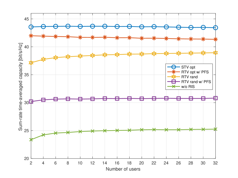
Figure 5: Sum-rate time-averaged capacity (left) and fairness index (right) versus the number of users $K$ (Example 1).

Figure 6: Sum-rate time-averaged capacity (left) and fairness index (right) versus the number of meta-atoms $Q$ (Example 1).

VI-A Example 1: Homogeneous users

Fig. 5 shows the sum-rate time-averaged capacity (left-side plot) and fairness (right-side plot) performance of the schemes under comparison in the case of homogeneous users as a function of the number of users $K$, with $Q=10\times 10$ meta-atoms. We observe that, except for the schemes requiring full CSIT, the sum-rate time-averaged capacity increases double logarithmically with the number of users $K$ in the system: this is the multiuser diversity effect [74]. The same effect is not visible for the “STV opt” and “RTV opt w/ PFS” downlinks since the logarithmic growth of the mean overall channel with $K$ is contrasted by the pilot overhead required to acquire full CSIT, which also depends on $K$. It is clear that the presence of an RIS leads to significant sum-rate gains with respect the “w/o RIS” case.

As expected, even thought the “STV opt” downlink allows to achieve the best sum-rate capacity performance, it requires full CSIT and, moreover, as in the scenario of “w/o RIS”, it becomes fairer and fairer as the number of users increases. In contrast, from the curves of “RTV rand”, one can argue that, compared to “STV opt”, a much fairer system can be obtained by introducing a rapidly time-varying randomization of the reflection response of the RIS, which also allows to highlight an interesting trade-off between performance and required amount of CSIT for downlink optimization. A $100\%$ fair system can be designed by using PFS. Obviously, such a fairness comes at the price of a sum-rate reduction: indeed, the sum-rate curves of the “RTV opt w/ PFS” and “RTV rand w/ PFS” systems are worse than those of their corresponding counterparts “STV opt” and “RTV rand”, respectively. Interestingly, although it involves partial CSIT only, the “RTV rand” downlink pays a mild performance gain with respect to “RTV opt w/ PFS” - which however requires full CSIT - by ensuring a fairness of nearly $100\%$ up to $18$ users and no smaller than $94\%$ up to $32$ users.

Fig. 6 shows the sum-rate time-averaged capacity (left-side plot) and fairness (right-side plot) performance of the schemes under comparison in the case of homogeneous users as a function of the number of meta-atoms $Q$, with $K=16$ users. Two additional interesting trends can be inferred from such figures. First, in accordance with our analysis in Subsection IV-A, the sum-rate time-averaged capacity of the schemes employing partial CSIT increases logarithmically with the number of meta-atoms $Q$ at the RIS, whereas the downlinks optimized with full CSIT exhibit a faster growth rate. Second, as the number of meta-atoms increases, the sum-rate capacity of “RTV opt w/ PFS” tends to that of “STV opt” by ensuring at the same time $100\%$ fairness, while $\mathcal{F}=100/16=6.25\%$ for the “STV opt” scheme.

Figure 7: Sum-rate time-averaged capacity (left) and fairness index (right) versus the number of users $K$ (Example 2).

Figure 8: Sum-rate time-averaged capacity (left) and fairness index (right) versus the number of meta-atoms $Q$ (Example 2).

VI-B Example 2: Heterogeneous users

Figs. 7 and 8 report the sum-rate time-averaged capacity (left-side plot) and fairness (right-side plot) performance of the schemes under comparison in the case of heterogeneous users. In Fig. 7, we set $Q=10\times 10$ meta-atoms, whereas we fix $K=16$ users in Fig. 8. Besides substantially confirming the above trends evidenced in Example 1, a behavior that is worth mentioning is the reduction in fairness of the “RTV rand” downlink, compared to the homogeneous case. Hence, we might argue that the randomization in both space and time of the reflection coefficients of the RIS leads to a fair resource allocation if there is no severe “near-far effect”, i.e., users that experience significantly different fading effects. It is apparent that, to cope with such an heterogeneous situation, the schemes employing PFS are forced to meaningfully cut down their sum-rate performance in order to fulfill the fairness constraint.

VII Conclusion and directions for future work

In this article, we have investigated the impact of a rapidly time-varying RIS on the resource allocation in a downlink multiuser system operating over slow fading channels.

The following results have been obtained:

1. Joint optimization of transmit powers and reflection coefficients of the RIS in the case of full CSIT leads to a slowly time-varying RIS, whose reflection response is updated with a rate that is (approximately) the inverse of the channel coherence time. In this case, only one user is scheduled within a channel coherence interval.

2. The assumption of full CSIT can be relaxed by randomizing the reflection coefficients of a rapidly time-varying RIS in both space and time domains, without paying a penalty in terms of multiuser diversity gain. The resulting resource allocation scheme requires partial CSIT only and ensures a certain fairness, since the randomization in time allows the transmitter to serve more than one user for each channel coherence time interval.

3. If the main design concern is to meet fairness among users while at the same time exploiting the multiuser diversity gain, then a rapidly time-varying RIS has to be employed in the downlink. In such a case, the temporal dimension of the RIS is beneficial not only in the partial CSIT scenario, but also in the full CSIT one.

This study demonstrates that, if acquisition of full CSIT is not possible in practice and/or the communication system has stringent requirements in terms of fairness, the exploitation of the temporal dimension of a rapidly time-varying RIS is instrumental in designing the downlink of a multiuser systems even in slow fading scenarios. We have considered single-antennas transmitter and receivers. In this respect, a first interesting research subject consists of extending the proposed framework to the case of multi-antenna terminals. In this case, the downlink is in general a nondegraded broadcast channel and sum capacity is achieved by using more sophisticated multiple access strategies than opportunistic time sharing, i.e., dirty-paper coding. An additional research direction involves investigating the benefits of a rapidly time-varying RIS in fast fading environments.

Francesco Verde (Senior Member, IEEE) received the Dr. Eng. degree summa cum laude in electronic engineering from the Second University of Napoli, Italy, in 1998, and the Ph.D. degree in information engineering from the University of Napoli Federico II, in 2002. Since December 2002, he has been with the University of Napoli Federico II, Italy. He first served as an Assistant Professor of signal theory and mobile communications and, since December 2011, he has served as an Associate Professor of telecommunications with the Department of Electrical Engineering and Information Technology. His research activities include reflected-power communications, orthogonal/non-orthogonal multiple-access techniques, wireless systems optimization, and physical-layer security. Prof. Verde has been involved in several technical program committees of major IEEE conferences in signal processing and wireless communications. He has served as Associate Editor for IEEE TRANSACTIONS ON VEHICULAR TECHNOLOGY since 2022. He was an Associate Editor of the IEEE TRANSACTIONS ON SIGNAL PROCESSING (from 2010 to 2014), IEEE SIGNAL PROCESSING LETTERS (from 2014 to 2018), IEEE TRANSACTIONS ON COMMUNICATIONS (from 2017 to 2022), and Senior Area Editor of the IEEE SIGNAL PROCESSING LETTERS (from 2018 to 2023), as well as Guest Editor of the EURASIP Journal on Advances in Signal Processing in 2010 and SENSORS MDPI in 2018-2022.

Donatella Darsena (Senior Member, IEEE) received the Dr. Eng. degree summa cum laude in telecommunications engineering in 2001, and the Ph.D. degree in electronic and telecommunications engineering in 2005, both from the University of Napoli Federico II, Italy. From 2001 to 2002, she worked as embedded system designer in the Telecommunications, Peripherals and Automotive Group, STMicroelectronics, Milano, Italy. In 2005 she joined the Department of Engineering at Parthenope University of Napoli, Italy and worked first as an Assistant Professor and then as an Associate Professor from 2005 to 2022. She is currently an Associate Professor in the Department of Electrical Engineering and Information Technology of the University of Napoli Federico II, Italy. Her research interests are in the broad area of signal processing for communications, with current emphasis on reflected-power communications, orthogonal and nonorthogonal multiple access techniques, wireless system optimization, and physical-layer security. Dr. Darsena has served as an Associate Editor for IEEE ACCESS since October 2018 and for IEEE SIGNAL PROCESSING LETTERS since 2020. She served first as an Associate Editor (from December 2016 to July 2019) and then as a Senior Area Editor (from August 2019 to July 2023) for IEEE COMMUNICATIONS LETTERS. Since July 2023, she has been an Executive Editor of IEEE COMMUNICATIONS LETTERS.

Vincenzo Galdi (Fellow, IEEE) received the Laurea degree (summa cum laude) in electrical engineering and the Ph.D. degree in applied electromagnetics from the University of Salerno, Italy, in 1995 and 1999, respectively. He has held several research-associate and visiting positions at abroad research institutions, including the European Space Research and Technology Centre, Noordwijk, The Netherlands; Boston University, Boston, MA, USA; the Massachusetts Institute of Technology, Cambridge, MA, USA; the California Institute of Technology, Pasadena, CA, USA; and The University of Texas at Austin, Austin, TX, USA. He is currently a Professor of electromagnetics with the Department of Engineering, University of Sannio, Benevento, Italy, where he leads the Fields & Waves Laboratory. He is the Co-Founder of the spinoff company MANTID srl, Benevento, and the startup company BioTag srl, Naples. He has co-edited two books and coauthored about 180 articles in peer-reviewed international journals, and is the co-inventor of thirteen patents. His research interests encompass wave interactions with complex structures and media, multiphysics metamaterials, smart propagation environments, optical sensing, and gravitational interferometry. Dr. Galdi is a Fellow of Optica (formerly OSA), a Senior Member of the LIGO Scientific Collaboration, and a member of the American Physical Society. He was a recipient of the Outstanding Associate Editor Award of IEEE Transactions on Antennas and Propagation in 2014 and the URSI Young Scientist Award in 2001. He has served as the Chair for the Technical Program Committee of the International Congress on Engineered Material Platforms for Novel Wave Phenomena in 2018, the Topical/Track Chair for the Technical Program Committee of the IEEE International Symposium on Antennas and Propagation and USNC-URSI Radio Science Meeting from 2016 to 2017 and from 2020 to 2023, and an organizer/chair for several topical workshops and special sessions. He has also served as a Track Editor from 2016 to 2020, a Senior Associate Editor from 2015 to 2016, and an Associate Editor from 2013 to 2014 of the IEEE Transactions on Antennas and Propagation. He is serving as an Associate Editor of Optics Express and Heliyon and a regular reviewer for many journals, conferences, and funding agencies.

References

- [1] C. Liaskos, S. Nie, A. Tsioliaridou, A. Pitsillides, S. Ioannidis, and I.F. Akyildiz, “A new wireless communication paradigm through software-controlled metasurfaces,” IEEE Commun. Magazine, vol. 56, pp. 162-169, Sep. 2018.
- [2] E. Basar, M. Di Renzo, J. De Rosny, M. Debbah, M. Alouini, and R. Zhang, “Wireless communications through reconfigurable intelligent surfaces,” IEEE Access, vol. 7, pp. 116753-116773, 2019.
- [3] M. Di Renzo et al., “Smart radio environments empowered by reconfigurable AI meta-surfaces: An idea whose time has come,” J. Wireless Commun. Network, 129 (2019), https://doi.org/10.1186/s13638-019-1438-9.
- [4] M. Di Renzo et al., “Smart radio environments empowered by reconfigurable intelligent surfaces: How it works, state of research, and the road ahead,” IEEE J. Select. Areas Commun., vol. 38, pp. 2450-2525, Nov. 2020.
- [5] W. Tang et al., “MIMO transmission through reconfigurable intelligent surface: System design, analysis, and implementation,” IEEE J. Select. Areas Commun., vol. 38, pp. 2683-2699, Nov. 2020.
- [6] W. Tang et al., “Wireless communications with reconfigurable intelligent surface: Path loss modeling and experimental measurement,” IEEE Trans. Wireless Commun., vol. 20, pp. 421-439, Jan. 2021.
- [7] T.J. Cui, M.Q. Qi, X. Wan, J. Zhao, and Q. Cheng, “Coding metamaterials, digital metamaterials and programmable metamaterials,” Light-Sci. Appl., vol. 3, e218, Oct. 2014.
- [8] C. Huang, B. Sun, W. Pan, J. Cui, X. Wu, and X. Luo, “Dynamical beam manipulation based on 2-bit digitally-controlled coding metasurface,” Sci. Rep., vol. 7, Feb. 2017, Art. no. 42302.
- [9] Y.B. Li et al., “Transmission-type 2-bit programmable metasurface for single-sensor and single-frequency microwave imaging,” Sci. Rep., vol. 6, Mar. 2016, Art. no. 23731.
- [10] L. Li et al., “Electromagnetic reprogrammable coding metasurface holograms,” Nature Commun., vol. 8, Aug. 2017, Art. no. 197.
- [11] X. Cai, Z. Zhou, and T.H. Tao, “Programmable vanishing multifunctional optics,” Adv. Sci., vol. 6, Feb. 2019, Art. no. 1801746.
- [12] S. Liu and T.J. Cui, “Concepts, working principles, and applications of coding and programmable metamaterials,” Adv. Opt. Mater., vol. 5, Nov. 2017, Art. no. 1700624.
- [13] D.F. Sievenpiper, J.H. Schaffner, H.J. Song, R.Y. Loo, and G. Tangonan, “Two-dimensional beam steering using an electrically tunable impedance surface,” IEEE Trans. Antennas Propag., vol. 51, pp. 2713-2722, 2003.
- [14] J.Y. Lau and S.V. Hum, “A wideband reconfigurable transmitarray element,” IEEE Trans. Antennas Propag., vol. 60, pp. 1303-1311, Mar. 2012.
- [15] L. Boccia, I. Russo, G. Amendola, G. Di Massa, “Multilayer antenna-filter antenna for beam-steering transmit-array applications,” IEEE Trans. Microw. Theory Tech., vol. 60, pp. 2287-2300, July 2012.
- [16] I.V. Shadrivov, P.V. Kapitanova, S.I. Maslovski, and Y.S. Kivshar, “Metamaterials controlled with light,” Phys. Rev. Lett., vol. 109, 083902, Aug. 2012.
- [17] X. Wu et al., “Active microwave absorber with the dual-ability of dividable modulation in absorbing intensity and frequency,” AIP Adv., vol. 3, 022114, Feb. 2013.
- [18] K. Chen et al., “A reconfigurable active Huygens’ metalens,” Adv. Mater., vol. 29, May 2017, Art. no. 1606422.
- [19] L. Zhang et al., “Dynamically realizing arbitrary multi-bit programmable phases using a 2-Bit time-domain coding metasurface,” IEEE Trans. Antennas Propag., vol. 68, pp. 2984-2992, Apr. 2020.
- [20] J. Zhao et al., “Programmable time-domain digital-coding metasurface for non-linear harmonic manipulation and new wireless communication systems,” Nat. Sci. Rev., vol. 6, pp. 231-238, Mar. 2019.
- [21] L. Zhang et al., “Space-time-coding digital metasurfaces,” Nature Commun., vol. 9, 4334, 2018.
- [22] A. Tennant and B. Chambers, “Time-switched array analysis of phase- switched screens,” IEEE Trans. Antennas Propag., vol. 57, pp. 808-812, Mar. 2009.
- [23] W. Kummer, A. Villeneuve, T. Fong, and F. Terrio, “Ultra-low sidelobes from time-modulated arrays,” IEEE Trans. Antennas Propag., vol. 11, pp. 633-639, Nov. 1963.
- [24] L. Zhang et al., “Breaking reciprocity with space-time-coding digital metasurfaces,” Adv. Mater., vol. 31, Oct. 2019, Art. no. 1904069.
- [25] J.Y. Dai, J. Zhao, Q. Cheng, and T.J. Cui, “Independent control of harmonic amplitudes and phases via a time-domain digital coding metasurface,” Light-Sci. Appl., vol. 7, Nov. 2018, Art. no. 90.
- [26] J.Y. Dai et al., “High-efficiency synthesizer for spatial waves based on space-time-coding digital metasurface,” Laser Photon. Rev., vol. 14, 8, Jun. 2020, Art. no. 1900133.
- [27] J.Y. Dai et al., “Arbitrary manipulations of dual harmonics and their wave behaviors based on space-time-coding digital metasurface,” Appl. Phys. Rev., vol. 7, 9, Dec. 2020, Art. no. 041408.
- [28] H. Rajabalipanah, A. Abdolali, S. Iqbal, L. Zhang, and T.J. Cui, “Analog signal processing through space-time digital metasurfaces,” Nanophotonics, vol. 10, pp. 1753-1764, 2021.
- [29] G. Castaldi, L. Zhang, M. Moccia, A.Y. Hathaway, W.X. Tang, T.J. Cui, and V. Galdi, “Joint multi-frequency beam shaping and steering via space–time-coding digital metasurfaces,” Adv. Funct. Mater., 31, 2007620, 2021.
- [30] L. Zhang et al., “A wireless communication scheme based on space- and frequency-division multiplexing using digital metasurfaces,” Nat. Electron., 4, pp. 218-227, 2021.
- [31] S. Taravati and G.V. Eleftheriades, “Microwave space-time-modulated metasurfaces,” ACS Photonics, 9, pp. 305-318, Jan. 2022.
- [32] J. Zhao et al., “Programmable time-domain digital-coding metasurface for non-linear harmonic manipulation and new wireless communication systems,” Natl. Sci. Rev., vol. 6, pp. 231-238, Mar. 2019.
- [33] X. Wang and C. Caloz, “Spread-spectrum selective camouflaging based on time-modulated metasurface,” IEEE Trans. Antennas Propag., vol. 69, pp. 286-295, Jan. 2021.
- [34] Y. Hadad, D.L. Sounas, and A. Alù, “Space-time gradient metasurfaces,” Phys. Rev. B, vol. 92, Sep. 2015, Art. no. 100304
- [35] S. Taravati and G.V. Eleftheriades, “Full-duplex nonreciprocal beam steering by time-modulated phase-gradient metasurfaces,” Phys. Rev. Appl., vol. 14, July 2020, Art. no. 014027.
- [36] S. Hu, F. Rusek, and O. Edfors,“Beyond massive MIMO: The potential of data transmission with large intelligent surfaces,” IEEE Trans. Signal Process., vol. 66, pp. 2746-2758, May 2018.
- [37] M. Jung, W. Saad, Y. Jang, G. Kong, and S. Choi, “Performance analysis of large intelligent surfaces (LISs): Asymptotic data rate and channel hardening effects,” IEEE Trans. Wireless Commun., vol. 19, pp. 2052-2065, Mar. 2020.
- [38] S. Li, B. Duo, X. Yuan, Y.-C. Liang, and M. Di Renzo, “Reconfigurable intelligent surface assisted UAV communication: Joint trajectory design and passive beamforming,” IEEE Wireless Commun. Lett., vol. 9, pp. 716-720, May 2020.
- [39] B. Di, H. Zhang, L. Song, Y. Li, Z. Han, and H.V. Poor, “Hybrid beamforming for reconfigurable intelligent surface based multi-user communications: Achievable rates with limited discrete phase shifts”, IEEE J. Select. Areas Commun., vol. 38, pp. 1809-1822, Aug. 2020.
- [40] C. Huang, R. Mo, and C. Yuen, “Reconfigurable intelligent surface assisted multiuser MISO systems exploiting deep reinforcement learning,” IEEE J. Select. Areas Commun., vol. 38, pp. 1839-1850, Aug. 2020.
- [41] M. Najafi, V. Jamali, R. Schober, and H.V. Poor, “Physics-based modeling and scalable optimization of large intelligent reflecting surfaces,” IEEE Trans. Commun., vol. 69, pp. 2673-2691, Apr. 2021.
- [42] A. Abrardo, D. Dardari, and M. Di Renzo, “Intelligent reflecting surfaces: Sum-rate optimization based on statistical position information,” IEEE Trans. Commun., vol. 69, pp. 7121-7136, Oct. 2021.
- [43] C. Pan, H. Ren, K. Wang, W. Xu, M. Elkashlan, A. Nallanathan, and L. Hanzo, “Multicell MIMO communications relying on intelligent reflecting surface”, vol. 19, pp. 5218-5233, Aug. 2020.
- [44] P. Wang, J. Fang, X. Yuan, Z. Chen, and H. Li, “Intelligent reflecting surface-assisted millimeter wave communications: Joint active and passive precoding design,” IEEE Trans. Veh. Technol., vol. 69, pp. 14960-14973, Dec. 2020.
- [45] C. Huang, A. Zappone, G.C. Alexandropoulos, M. Debbah, and C. Yuen, “Reconfigurable intelligent surfaces for energy efficiency in wireless communication,” IEEE Trans. Wireless Commun., vol. 18, pp. 4157-4170, Aug. 2019.
- [46] W. Yan, X. Yuan, and X. Kuai, “Passive beamforming and information transfer via large intelligent surface,” IEEE Wireless Commun. Lett., vol. 9, pp. 533-537, Apr. 2020.
- [47] Q.-U.-A. Nadeem, A. Kammoun, A. Chaaban, M. Debbah, and M.-S. Alouini, “Asymptotic max-min SINR analysis of reconfigurable intelligent surface assisted MISO systems,” in revision on IEEE Trans. Wireless Commun., vol. 19, pp. 7748-7764, Dec. 2020.
- [48] A. Zappone, M. Di Renzo, F. Shams, X. Qian, and M. Debbah, “Overhead-aware design of reconfigurable intelligent surfaces in smart radio environments,” IEEE Trans. Wireless Commun., vol. 20, pp. 126-141, Jan. 2021.
- [49] G. Zhou, C. Pan, H. Ren, K. Wang, M. Di Renzo, and A. Nallanathan, “Robust beamforming design for intelligent reflecting surface aided MISO communication systems”, IEEE Wireless Commun. Lett., vol. 9, pp. 1658-1662, Oct. 2020.
- [50] J. He, H. Wymeersch, and M. Juntti, “Channel estimation for RIS-aided mmwave MIMO systems via atomic norm minimization,” IEEE Trans. Wireless Commun., vol. 20, pp. 5786-5797, Sep. 2021.
- [51] D. Dardari, N. Decarli, A. Guerra and F. Guidi, “LOS/NLOS near-field localization with a large reconfigurable intelligent surface,” IEEE Trans. Wireless Commun., vol. 21, pp. 4282-4294, June 2022.
- [52] O. Yurduseven, S.D. Assimonis, and M. Matthaiou, “Intelligent reflecting surfaces with spatial modulation: An electromagnetic perspective,” IEEE Open J. Commun. Soc., vol. 1, pp. 1256-1266, 2020.
- [53] M. Mizmizi, D. Tagliaferri, and U. Spagnolini, “Wireless communications with space-time modulated metasurfaces”, arXiv:2302.08310, Feb. 2023.
- [54] D. Bertsekas, Nonlinear Programming. Belmont, MA: Athena Scientific, 1999.
- [55] F.P. Kelly, A.K. Maulloo, and D.K.H. Tan., “Rate control in communication networks: Shadow prices, proportional fairness and stability,” J. of the Operational Research Society, vol. 49, pp. 237-252, Apr. 1998.
- [56] MIMO AH Summary, [Online]. Available: http://www.3gpp.org/ftp/tsg_ran/WG1_RL1/TSGR1_49b, R1-073225, Ad Hoc Chairman.
- [57] 3GPP TS 38.211 (2019), “NR; Physical channels and modulation (Release 15),” V15.7.0 (2019-9).
- [58] J.G. Proakis, Digital Communications. New York, NY, USA: McGraw-Hill, 2001.
- [59] X. Ding et al., “Metasurface holographic image projection based on mathematical properties of Fourier transform”, PhotoniX, art. no. 16, pp. 1-12, 2020.
- [60] J. Liao et al., “Independent manipulation of reflection amplitude and phase by a single-layer reconfigurable metasurface”Adv. Optical Mater., 2101551, pp. 1-9, 2021.
- [61] Q.R. Hong et al., “Programmable amplitude-coding metasurface with multifrequency modulations”Adv. Intell. Syst., 3, 2000260, pp. 1-9, 2021.
- [62] H. Li et al., “The design of programmable transmitarray with independent controls of transmission amplitude and phase”, IEEE Trans. Antennas Propag., vol. 70, pp. 8086-8099, Sep. 2022.
- [63] B. Wu, A. Sutinjo, M.E. Potter, and M. Okoniewski, “On the selection of the number of bits to control a digital MEMS reflectarray,” IEEE Antennas Wirel. Propag. Lett., vol. 7, pp. 183-186, 2008.
- [64] 3GPP, “NR; Physical channels and modulation (Release 15),” TS 38.211, July 2018.
- [65] L. Wang et al., “A review of THz modulators with dynamic tunable metasurfaces,” Nanomaterials, vol. 9, p. 965, July 2019.
- [66] P.F. Driessen and G. Foschini, “On the capacity formula for multiple input-multiple output wireless channels: A geometric interpretation,” IEEE Trans. Commun., vol. 47, pp. 173-176, Feb. 1999.
- [67] M.C. Gursoy, “On the capacity and energy efficiency of training-based transmissions over fading channels,” IEEE Trans. Inf. Theory, vol. 55, pp. 4543–4567, Oct. 2009.
- [68] A.L. Swindlehurst, G. Zhou, R. Liu, C. Pan, and M. Li, “Channel estimation with reconfigurable intelligent surfaces - A general framework,” Proc. IEEE, vol. 110, pp. 1312–1338, Sep. 2022.
- [69] 3GPP, “Evolved universal terrestrial radio access (E-UTRA); Physical layer procedures for control (Release 15),” TS 38.213, Dec. 2017.
- [70] A. Bletsas, A. Khisti, D.P. Reed, and A. Lippman, “A simple cooperative diversity method based on network path selection,” IEEE J. Select. Areas Commun., vol. 24, pp. 659–672, Mar. 2006.
- [71] S.M. Kay, Fundamentals of Statistical Signal Processing, Vol. 2: Detection Theory. Prentice Hall PTR, 1998.
- [72] D.N.C. Tse, “Optimal power allocation over parallel Gaussian channels,” in Proc. Int. Symp. Information Theory, Ulm, Germany, June 1997.
- [73] J. Jang and K.B. Lee, “Transmit power adaptation for multiuser OFDM systems,” IEEE Trans. Signal Process., vol. 21, pp. 171–178, Feb. 2003.
- [74] D. Tse and and P. Viswanath, Fundamentals of Wireless Communication. Cambridge University Press, New York, 2005.
- [75] R.A. Horn and C.R. Johnson, Matrix Analysis. New York: Cambridge Univ. Press, 1990.
- [76] Q. Wu and R. Zhang, “Beamforming optimization for wireless network aided by intelligent reflecting surface with discrete phase shifts,” IEEE Trans. Commun., vol. 68, pp. 1838–1851, Mar. 2020.
- [77] M.-M. Zhao, Q. Wu, M.-J. Zhao, and R. Zhang, “Exploiting amplitude control in intelligent reflecting surface aided wireless communication with imperfect CSI,” IEEE Trans. Commun., vol. 69, pp. 4216–4231, June 2021.
- [78] J. Kim, J. Choi, J. Joung and Y.-C. Liang, “Modified block coordinate descent method for intelligent reflecting surface-aided space-time line coded systems,” IEEE Wireless Commun. Lett., vol. 11, pp. 1820–1824, Sep. 2022.
- [79] S.A. Tegos, D. Tyrovolas, P.D. Diamantoulakis, C.K. Liaskos, and G.K. Karagiannidis, “On the distribution of the sum of double-Nakagami- random vectors and application in randomly reconfigurable surfaces,” IEEE Trans. Veh. Technol., vol. 71, pp. 7297–7307, July 2022.
- [80] M.R. Leadbetter, “Extreme value theory under weak mixing conditions,” Studies in Probability Theory, MAA Studies in Mathematics, pp. 46-110, 1978.
- [81] E.J. Gumbel, Statistics of Extremes. Columbia University Press, 1958.
- [82] S. Kalyani and R.M. Karthik, “The asymptotic distribution of maxima of independent and identically distributed sums of correlated or non-identical gamma random variables and its applications,” IEEE Trans. Commun., vol. 60, pp. 2747-2758, Sep. 2012.
- [83] R. Jain, D. Chiu, and W. Hawe, “A quantitative measure of fairness and discrimination for resource allocation in shared computer systems,” DEC Research Report TR-301, Sept. 1984.
- [84] J. Mo and J. Walrand, “Fair end-to-end window-based congestion control,” IEEE/ACM Trans. Netw., vol. 8, pp. 556-567, Oct. 2000.
- [85] S.W. Ellingson, “Path loss in reconfigurable intelligent surface-enabled channels,” in Proc. IEEE Annual Int. Symp. Personal, Indoor and Mobile Radio Commun. (PIMRC), Helsinki, Finland, Sep. 2021, pp. 829-835.