Some results on Continuous dependence of fractal functions on the Sierpiński gasket

Abstract.

In this article, we show that $\displaystyle\alpha$-fractal functions defined on Sierpiński gasket (denoted by $\displaystyle\triangle$) depend continuously on the parameters involved in the construction. In the latter part of this article, the continuous dependence of parameters on $\displaystyle\alpha$-fractal functions defined on $\displaystyle\triangle$ is shown graphically.

1. Introduction

In the field of Numerical Analysis, the computational implications of interpolation have been a major concern for many years. The theory of interpolation has evolved throughout the development of classical approximation theory. Various interpolation techniques are used in Numerical Analysis and Classical Approximation Theory, and they are based on polynomial, trigonometric, spline, and rational functions. Based on the underlying idea of the model under investigation, these techniques can be applied to a specific data set. While nonrecursive interpolation techniques in the literature almost always produce smooth interpolants, it should be emphasized that they are not all recursive. There are a great number of real-world phenomena and experimental signals that are confusing, and sometimes their traces appear smooth. Due to their non-differentiability and complexity, a simple mathematical framework may not adequately describe their smallest geometric complexity. In order to produce an interpolant with a more complex geometric structure, it is necessary to develop a novel interpolation approach. Univariate real-valued interpolation functions constructed on a compact interval in $\displaystyle\mathbb{R}$ were first proposed by Barnsley [3]. These are referred to as Fractal Interpolation Functions (FIFs for short), and their construction is based on the Iterated Function System (IFS) theory [10]. In [3], the groundbreaking research on fractal interpolation has attracted a lot of interest in the literature and is currently going strong. The author of [16] demonstrated that the FIFs theory can be used to construct a family of continuous functions with fractal properties from a given continuous function.

A number of studies have exposed several significant characteristics of FIFs, including their smoothness, stability, one-sided approximation property and constraint approximation property, as well as their box dimension and Hausdorff dimension. There are several research articles available on various types of FIFs, see, for instance, [5, 8, 12, 13, 17, 19]. Numerous studies reveal several significant aspects of FIFs, such as their smoothness, stability, one-sided approximation property and constrained approximation properties, as well as box dimension and Hausdorff dimension of their graphs. Celik et al. [4] expanded the notion of FIFs to incorporate interpolation of a data set on $\displaystyle\triangle$. Following this article, Ruan [24] developed FIFs on post critically finite self-similar sets. Kigami [14] is credited with having introduced and analysed these sets. On $\displaystyle\triangle$, Ri and Ruan [23] defined several fundamental characteristics of a space of FIFs. The fractal dimensions of FIFs defined on various domains have been thoroughly investigated in numerous articles, see, for instance, [6, 7, 9, 11, 18, 21, 25, 27, 28, 32, 31]. Recently, Mohapatra et al. [15] introduced a concept that generalised the notions of the Kannan map and contraction. In [20], Prasad and Verma have constructed the FIFs on the product of two Sierpiński gaskets.

We denote the space of all the real-valued continuous functions defined on $\displaystyle\triangle$ by $\displaystyle C(\triangle,\mathbb{R})$ and graph of $\displaystyle f$ by $\displaystyle graph(f)$ throughout this paper.

2. Fractal interpolation function on the Sierpiński gasket

We begin by providing a brief overview of the relevant concepts and an introduction to $\displaystyle\triangle$. The reader may refer to [2, 22, 26, 30] for further information. We begin by recalling an established $\displaystyle\triangle$ construction based on IFS. Consider a set $\displaystyle V_{0}=\left\{x_{1},x_{2},x_{3}\right\}$ such that points in $\displaystyle V_{0}$ have equal distances from each other. Corresponding to each point of $\displaystyle V_{0}$, define the contraction map $\displaystyle u_{i}$ on $\displaystyle\mathbb{R}^{2}$ as follows:

$$u_{i}(t)=\frac{1}{2}\left(t+x_{i}\right),$$

where $\displaystyle i=1,2,3$. Then, three contraction maps together with the plane constitute an IFS, which produces $\displaystyle\triangle$ as an attractor, i.e.,

$$\triangle=\bigcup_{i=1}^{3}u_{i}(\triangle).$$

Define $\displaystyle V_{1}$ by $\displaystyle V_{1}=\left\{x_{1},x_{2},x_{3},u_{1}\left(x_{2}\right),u_{2}\left(x_{3}\right),u_{3}\left(x_{1}\right)\right\}$. Let us consider a continuous function $\displaystyle f:\triangle\rightarrow\mathbb{R}$. Let $\displaystyle U=\triangle\times\mathbb{R}$ and define maps $\displaystyle H_{i}:U\rightarrow U$ by

$$H_{i}(t,x)=\left(u_{i}(t),M_{i}(t,x)\right),i=1,2,3,$$

where $\displaystyle M_{i}(t,x):\triangle\times\mathbb{R}\rightarrow\mathbb{R}$ is a contraction map in the last variable, that is,

$$\left|M_{i}(.,x)-M_{i}\left(.,x^{\prime}\right)\right|\leq c\left|x-x^{\prime}\right|$$

with $\displaystyle M_{i}\left(p_{j},f\left(p_{j}\right)\right)=f\left(u_{i}\left(p_{j}\right)\right)$. In particular, we take

$$M_{i}(t,x)=\alpha_{i}x+f\left(u_{i}(t)\right)-\alpha_{i}b(t),$$

where $\displaystyle b\in C(\triangle,\mathbb{R})$ is base function and $\displaystyle f\in C(\triangle,\mathbb{R})$ original function such that $\displaystyle b\left(p\right)=f\left(p\right)~{}\forall~{}p\in V_{0}$, and scale vector $\displaystyle\alpha_{i}\in\mathbb{R}$ with $\displaystyle\left|\alpha_{i}\right|_{\infty}<1$. Thus, We have an IFS $\displaystyle\mathcal{J}:=\left\{U,H_{i}:i=1,2,3\right\}$.

Theorem 2.1.

[1] Let $\displaystyle f\in C(\triangle,\mathbb{R})$, and $\displaystyle b\in C(\triangle,\mathbb{R})$. Then, above defined IFS $\displaystyle\mathcal{J}$ has a unique attractor $\displaystyle graph(f^{\alpha})$. The set $\displaystyle graph(f^{\alpha})$ is the graph of a continuous function $\displaystyle f^{\alpha}:\triangle\rightarrow\mathbb{R}$, which satisfies $\displaystyle\left.f^{\alpha}\right|_{V_{1}}=\left.f\right|_{V_{1}}$. Furthermore, we have the following functional equation

$$f^{\alpha}(t)=f(t)+\alpha_{i}\left(f^{\alpha}-b\right)\left(u_{i}^{-1}(t)\right)~{}\forall~{}t\in u_{i}(\triangle),i\in\{1,2,3\}.$$ (1)

3. Continuous dependence on parameter $\displaystyle\alpha$ AND $\displaystyle b$

Let $\displaystyle f\in C(\triangle,\mathbb{R})$. Define a map $\displaystyle W$ from $\displaystyle S$ to $\displaystyle C(\triangle,\mathbb{R})$ by

$$W(\alpha)=f_{b}^{\alpha},$$

where $\displaystyle S=\left\{\alpha\in\mathbb{R}^{3}:|\alpha|_{\infty}\leq r<1\right.$ and $\displaystyle r$ is a fixed number$\displaystyle\}$ and $\displaystyle f_{b}^{\alpha}$ is $\displaystyle\alpha$-fractal function associated with $\displaystyle f$ with respect to $\displaystyle b$ and the scale vector $\displaystyle\alpha$.

Theorem 3.1.

For fixed $\displaystyle f\in C(\triangle,\mathbb{R})$ and for suitable $\displaystyle b\in C(\triangle,\mathbb{R})$, the map $\displaystyle W:S\rightarrow C(\triangle,\mathbb{R})$ is continuous.

Proof.

The fixed point theory says that for a fixed a scale vector $\displaystyle\alpha$, and $\displaystyle b$, the map $\displaystyle f_{b}^{\alpha}$ is unique. Further, being fixed point of RB- operator, $\displaystyle f_{b}^{\alpha}$ satisfies the functional equation:

$$f_{b}^{\alpha}(t)=f(t)+\alpha_{i}\left(f_{b}^{\alpha}-b\right)\circ u_{i}^{-1}(t),~{}\forall~{}t\in u_{i}(\triangle),i\in\{1,2,3\}.$$

It is obvious that $\displaystyle W$ is well defined. Let $\displaystyle\alpha\in S$, then from the above functional equation, we have

$$W(\alpha)(t)=f_{b}^{\alpha}(t)=f(t)+\alpha_{i}\left(f_{b}^{\alpha}-b\right)\circ u_{i}^{-1}(t),~{}\forall~{}t\in u_{i}(\triangle),i\in\{1,2,3\}$$

and for $\displaystyle\beta\in S$,

$$W(\beta)(t)=f_{b}^{\beta}(t)=f(t)+\beta_{i}\left(f_{b}^{\beta}-b\right)\circ u_{i}^{-1}(t),~{}\forall~{}t\in u_{i}(\triangle),i\in\{1,2,3\}.$$

We shall show that $\displaystyle W$ is continuous at $\displaystyle\alpha$. For this, subtract one from other of the above two equations, for $\displaystyle t\in u_{i}(\triangle)$, we have

$$f_{b}^{\alpha}(t)-f_{b}^{\beta}(t) =\left[f(t)+\alpha_{i}\left(f_{b}^{\alpha}-b\right)\circ u_{i}^{-1}(t)\right]-\left[f(t)+\beta_{i}\left(f_{b}^{\beta}-b\right)\circ u_{i}^{-1}(t)\right]$$ (2)

$$=\left[\alpha_{i}f_{b}^{\alpha}\left(u_{i}^{-1}(t)\right)-\beta_{i}f_{b}^{\beta}\left(u_{i}^{-1}(t)\right)\right]+\left(\beta_{i}-\alpha_{i}\right)b\circ u_{i}^{-1}(t)$$

$$=\left[\alpha_{i}f_{b}^{\alpha}-\beta_{i}f_{b}^{\alpha}+\beta_{i}f_{b}^{\alpha}-\beta_{i}f_{b}^{\beta}\right]\circ u_{i}^{-1}(t)+\left(\beta_{i}-\alpha_{i}\right)b\circ u_{i}^{-1}(t)$$

$$=\left[\left(\alpha_{i}-\beta_{i}\right)f_{b}^{\alpha}+\beta_{i}\left(f_{b}^{\alpha}-f_{b}^{\beta}\right)\right]\circ u_{i}^{-1}(t)+\left(\beta_{i}-\alpha_{i}\right)b\circ u_{i}^{-1}(t).$$

Now, using triangle inequality and definition of uniform norm, we have

$$\left|f_{b}^{\alpha}(t)-f_{b}^{\beta}(t)\right| \leq\left|\left[\left(\alpha_{i}-\beta_{i}\right)f_{b}^{\alpha}+\beta_{i}\left(f_{b}^{\alpha}-f_{b}^{\beta}\right)\right]\circ u_{i}^{-1}(t)\right|+\left|\left(\beta_{i}-\alpha_{i}\right)b\circ u_{i}^{-1}(t)\right|$$ (3)

$$\leq|\alpha-\beta|_{\infty}\left\|f_{b}^{\alpha}\right\|_{\infty}+|\beta|_{\infty}\left\|f_{b}^{\alpha}-f_{b}^{\beta}\right\|_{\infty}+|\beta-\alpha|_{\infty}\|b\|_{\infty}$$

$$=|\alpha-\beta|_{\infty}\left(\left\|f_{b}^{\alpha}\right\|_{\infty}+\|b\|_{\infty}\right)+|\beta|_{\infty}\left\|f_{b}^{\alpha}-f_{b}^{\beta}\right\|_{\infty}.$$

It follows that, for all $\displaystyle t\in\triangle$, we get

$$\left|f_{b}^{\alpha}(t)-f_{b}^{\beta}(t)\right|\leq|\alpha-\beta|_{\infty}\left(\left\|f_{b}^{\alpha}\right\|_{\infty}+\|b\|_{\infty}\right)+|\beta|_{\infty}\left\|f_{b}^{\alpha}-f_{b}^{\beta}\right\|_{\infty}.$$ (4)

The above implies that

$$\left\|f_{b}^{\alpha}-f_{b}^{\beta}\right\|_{\infty}\leq|\alpha-\beta|_{\infty}\left(\left\|f_{b}^{\alpha}\right\|_{\infty}+\|b\|_{\infty}\right)+|\beta|_{\infty}\left\|f_{b}^{\alpha}-f_{b}^{\beta}\right\|_{\infty}.$$ (5)

Using $\displaystyle 1-|\beta|_{\infty}\geq 1-r$, finally we have

$$\|W(\alpha)-W(\beta)\|_{\infty}=\|f_{b}^{\alpha}-f_{b}^{\beta}\|_{\infty}\leq\frac{|\alpha-\beta|_{\infty}}{1-r}\left(\left\|f_{b}^{\alpha}\right\|_{\infty}+\|b\|_{\infty}\right).$$ (6)

Since $\displaystyle\alpha$ is fixed and $\displaystyle\left\|f_{b}^{\alpha}\right\|_{\infty}$ is bounded, we have $\displaystyle W$ is continuous at $\displaystyle\alpha$. Since $\displaystyle\alpha$ was taken arbitrarily, hence, $\displaystyle W$ is continuous on $\displaystyle S$. ∎

Theorem 3.2.

Let $\displaystyle f\in C(\triangle,\mathbb{R})$ and scale vector $\displaystyle\alpha\in\mathbb{R}^{3}$ with $\displaystyle|\alpha|_{\infty}<1$ and $\displaystyle X_{f}=\left\{b\in C(\triangle,\mathbb{R}):\left.b\right|_{V_{0}}=\left.f\right|_{V_{0}}\right\}$. Then the map $\displaystyle T:X_{f}\rightarrow C(\triangle,\mathbb{R})$ defined by $\displaystyle T(b)=f_{b}^{\alpha}$ is Lipschitz continuous.

Proof.

We know that for a scale vector $\displaystyle\alpha$ and a suitable function $\displaystyle b:\triangle\rightarrow\mathbb{R}$, the function $\displaystyle f_{b}^{\alpha}$ is unique. Further, being fixed point of $\displaystyle\mathrm{RB}$ - operator, $\displaystyle f_{b}^{\alpha}$ satisfies the functional equation:

$$f_{b}^{\alpha}(t)=f(t)+\alpha_{i}\left(f_{b}^{\alpha}-b\right)\circ u_{i}^{-1}(t),~{}\forall~{}t\in u_{i}(\triangle),i\in\{1,2,3\}.$$

It is obvious that $\displaystyle T$ is well defined. Let $\displaystyle b,c\in X_{f}$ then from the above functional equation, we have

$$T(b)(t)=f_{b}^{\alpha}(t)=f(t)+\alpha_{i}\left(f_{b}^{\alpha}-b\right)\circ u_{i}^{-1}(t),~{}\forall~{}t\in u_{i}(\triangle),i\in\{1,2,3\}.$$

and

$$T(c)(t)=f_{c}^{\alpha}(t)=f(t)+\alpha_{i}\left(f_{c}^{\alpha}-c\right)\circ u_{i}^{-1}(t),~{}\forall~{}t\in u_{i}(\triangle),i\in\{1,2,3\}.$$

On subtracting one from other of the above two equations, we get for $\displaystyle t\in u_{i}(\triangle)$

$$f_{b}^{\alpha}(t)-f_{c}^{\alpha}(t) =\left[f(t)+\alpha_{i}\left(f_{b}^{\alpha}-b\right)\circ u_{i}^{-1}(t)\right]-\left[f(t)+\alpha_{i}\left(f_{c}^{\alpha}-c\right)\circ u_{i}^{-1}(t)\right]$$

$$=\alpha_{i}\left(f_{b}^{\alpha}-f_{c}^{\alpha}\right)\circ u_{i}^{-1}(t)+\alpha_{i}(c-b)\circ u_{i}^{-1}(t).$$

Now using triangle inequality and definition of uniform norm, we have

$$\left|f_{b}^{\alpha}(t)-f_{c}^{\alpha}(t)\right| =\left|\alpha_{i}\left(f_{b}^{\alpha}-f_{c}^{\alpha}\right)\circ u_{i}^{-1}(t)+\alpha_{i}(c-b)\circ u_{i}^{-1}(t)\right|$$

$$\leq\left|\alpha_{i}\left(f_{b}^{\alpha}-f_{c}^{\alpha}\right)\circ u_{i}^{-1}(t)\right|+\left|\alpha_{i}(c-b)\circ u_{i}^{-1}(t)\right|$$

$$\leq|\alpha|_{\infty}\left\|f_{b}^{\alpha}-f_{c}^{\alpha}\right\|_{\infty}+|\alpha|_{\infty}\|c-b\|_{\infty}.$$

The above inquality holds for all $\displaystyle t\in\triangle$, therefore, we write

$$\left\|f_{b}^{\alpha}-f_{c}^{\alpha}\right\|_{\infty}\leq|\alpha|_{\infty}\left\|f_{b}^{\alpha}-f_{c}^{\alpha}\right\|_{\infty}+|\alpha|_{\infty}\|c-b\|_{\infty}.$$

This can be recasted as, $\displaystyle\left\|f_{b}^{\alpha}-f_{c}^{\alpha}\right\|_{\infty}\leq\frac{|\alpha|_{\infty}}{1-|\alpha|_{\infty}}\|b-c\|_{\infty}$. It follows that

$$\|T(b)-T(c)\|_{\infty}\leq\frac{|\alpha|_{\infty}}{1-|\alpha|_{\infty}}\|b-c\|_{\infty},$$

which shows that $\displaystyle T$ is a Lipschitz continuous map with Lipschitz constant $\displaystyle\frac{|\alpha|_{\infty}}{1-|\alpha|_{\infty}}$. ∎

Next, we plot the $\displaystyle graph(f_{b}^{\alpha})$ for different values of parameters, that is, original function, base function and scale vector. One can easily identify the variation in these graphs by changing the values of parameters. Hence, $\displaystyle graph(f_{b}^{\alpha})$ depends on these parameters.

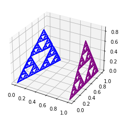
$\displaystyle graph(f_{b}^{\alpha})$ at $\displaystyle\alpha=0.1$

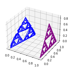
$\displaystyle graph(f_{b}^{\alpha})$ at $\displaystyle\alpha=0.3$

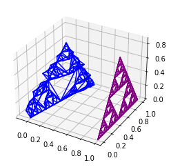
$\displaystyle graph(f_{b}^{\alpha})$ at $\displaystyle\alpha=0.6$

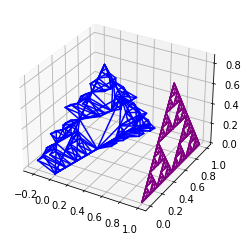
$\displaystyle graph(f_{b}^{\alpha})$ at $\displaystyle\alpha=0.9$

Figure 1. $\displaystyle graph(f_{b}^{\alpha})$ for the various values of the $\displaystyle\alpha$, where $\displaystyle b(x,y)=\frac{x}{4}+\frac{y}{9}-1.3y(x-0.5)$, $\displaystyle f(x,y)=\frac{x}{4}+\frac{y}{9}$.

$\displaystyle graph(f_{b}^{\alpha})$ at $\displaystyle\alpha=0.1$

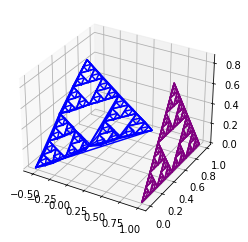
$\displaystyle graph(f_{b}^{\alpha})$ at $\displaystyle\alpha=0.3$

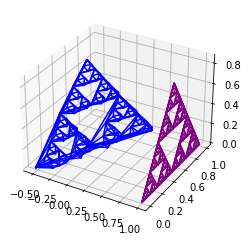
$\displaystyle graph(f_{b}^{\alpha})$ at $\displaystyle\alpha=0.6$

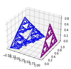
$\displaystyle graph(f_{b}^{\alpha})$ at $\displaystyle\alpha=0.9$

Figure 2. $\displaystyle graph(f_{b}^{\alpha})$ for the various values of the $\displaystyle\alpha$, where $\displaystyle b(x,y)=sin(x+3.7)+1.3x-x^{2}y+0.866x^{2}+xy-0.866x$, $\displaystyle f(x,y)=sin(x+3.7)+1.3x$.

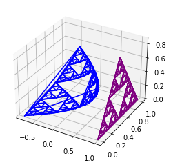
$\displaystyle graph(f_{b}^{\alpha})$ at $\displaystyle\alpha=0.1$

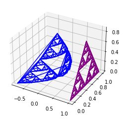
$\displaystyle graph(f_{b}^{\alpha})$ at $\displaystyle\alpha=0.3$

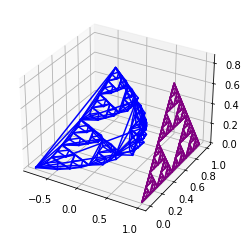
$\displaystyle graph(f_{b}^{\alpha})$ at $\displaystyle\alpha=0.6$

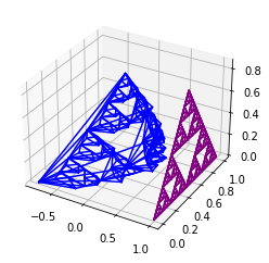
$\displaystyle graph(f_{b}^{\alpha})$ at $\displaystyle\alpha=0.9$

Figure 3. $\displaystyle graph(f_{b}^{\alpha})$ for the various values of the $\displaystyle\alpha$, where $\displaystyle b(x,y)=cos(2x+5)+sin(x+2.7)-1.5+1.3x-x^{2}y+0.866x^{2}+xy-0.866x$, $\displaystyle f(x,y)=cos(2x+5)+sin(x+2.7)-1.5+1.3x$.

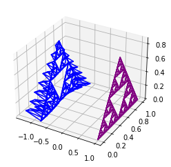
$\displaystyle graph(f_{b}^{\alpha})$ at $\displaystyle\alpha=0.1$

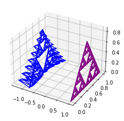
$\displaystyle graph(f_{b}^{\alpha})$ at $\displaystyle\alpha=0.3$

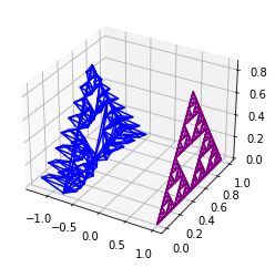
$\displaystyle graph(f_{b}^{\alpha})$ at $\displaystyle\alpha=0.6$

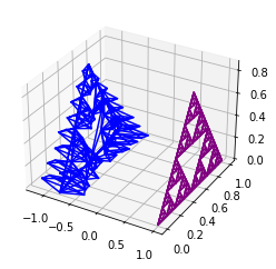
$\displaystyle graph(f_{b}^{\alpha})$ at $\displaystyle\alpha=0.9$

Figure 4. $\displaystyle graph(f_{b}^{\alpha})$ for the various values of the $\displaystyle\alpha$, where $\displaystyle b(x,y)=cos(100x+5)+sin(x+2.7)-1.5+1.3x-x^{2}y+0.866x^{2}+xy-0.866x$, $\displaystyle f(x,y)=cos(100x+5)+sin(x+2.7)-1.5+1.3x$.

4. Declaration

Funding. Not applicable.

Conflicts of interest. We do not have any conflict of interest.

Availability of data and material. Not applicable.

Code availability. Not applicable.

Authors’ contributions. Each author contributed equally in this manuscript.

References

- [1] V. Agrawal, T. Som, Fractal dimension of -fractal function on the Sierpiński Gasket, Eur. Phys. J. Spec. Top. 230, 3781-3787 (2021)
- [2] V. Agrawal, T. Som, -approximation using fractal functions on the Sierpiński Gasket, Results Math 77(2), 1-17 (2022)
- [3] M.F. Barnsley, Fractal functions and interpolation, Constr. Approx. 2 (1986) 303–329.
- [4] D. Celik, S. Kocak, Y. Özdemir, Fractal interpolation on the Sierpiński Gasket, J. Math. Anal. Appl. 337 (1), 343-347 (2008)
- [5] S. Chandra, S. Abbas, The calculus of bivariate fractal interpolation surfaces, Fractals 29(3) (2020)
- [6] S. Chandra, S. Abbas, Analysis of fractal dimension of mixed Riemann-Liouville integral, Numerical Algorithms 158, 1-26 (2022) https://doi.org/10.1007/s11075-022-01290-2
- [7] S. Chandra, S. Abbas, On fractal dimensions of fractal functions using functions spaces, Bull. Aust. Math. Soc. 1-11 (2022)
- [8] S. Chandra, S. Abbas, S. Verma, Bernstein Super Fractal Interpolation Function for Countable Data Systems, Numerical Algorithms (2022) https://doi.org/10.1007/s11075-022-01398-5
- [9] K. J. Falconer, Fractal Geometry: Mathematical Foundations and Applications, John Wiley Sons Inc., New York, 1999
- [10] J. E. Hutchinson, Fractals and self similarity, Indiana Uni. Math. J. 30(5), 713-747 (1981)
- [11] S. Jha, S. Verma, Dimensional Analysis of -Fractal Functions, Results Math 76(4), 1-24 (2021)
- [12] S. Jha, S. Verma, A. K. B. Chand, Non-stationary zipper -fractal functions and associated fractal operator, Fract Calc Appl Anal 25, 1527–1552 (2022)
- [13] S. Verma, S. Jha, A Study on Fractal Operator Corresponding to Non-stationary Fractal Interpolation Functions, Frontiers of Fractal Analysis Recent Advances and Challenges, 50-66 (2022)
- [14] J. Kigami, Analysis on Fractals, Cambridge University Press, Cambridge (2001)
- [15] R. N. Mohapatra, M. A. Navascues, M.V. Sebastian and S. Verma, Iteration of operators with contractive mutual relations of Kannan type, Mathematics 10(15), 2632 (2022)
- [16] M. A. Navascués, Fractal polynomial interpolation, Z. Anal. Anwend. 24(2), 401-418 (2005)
- [17] M. A. Navascues, S. Verma, Non-stationary alpha-fractal surfaces, Mediterranean Journal of Mathematics 20(1) (2023) 48.
- [18] M. Pandey, T. Som, S. Verma, Fractal dimension of Katugampola fractional integral of vector-valued functions, Eur. Phys. J. Spec. Top. 230, 3807–3814 (2021)
- [19] S. A. Prasad, Node insertion in Coalescence Fractal Interpolation Function, Chaos, Solitons and Fractals 49, 16-20 (2013)
- [20] S. A. Prasad, S. Verma, Fractal interpolation functions on products of the Sierpinski gaskets, Chaos, Solitons and Fractals 166 (2023) 112988
- [21] A. Priyadarshi, Lower bound on the Hausdorff dimension of a set of complex continued fractions, J. Math. Anal. Appl. 449(1), 91-95 (2017)
- [22] S.-I. Ri, Fractal functions on the Sierpiński gasket, Chaos, Solitons and Fractals 138 (2020)
- [23] S.-G. Ri, H.-J. Ruan, Some properties of fractal interpolation functions on Sierpinski gasket, J. Math. Anal. Appl. 380(1), 313-322 (2011)
- [24] H.-J. Ruan, Fractal interpolation functions on post critically finite self-similar sets, Fractals 18, 119-125 (2010)
- [25] A. Sahu, A. Priyadarshi, On the box-counting dimension of graphs of harmonic functions on the Sierpiński gasket, J. Math. Anal. Appl. 487(2), (2020)
- [26] R. S. Strichartz, Differential Equations on Fractals, Princeton University Press, Princeton, NJ, 2006
- [27] M. Verma, A. Priyadarshi, Graphs of continuous functions and fractal dimension. arXiv preprint arxiv.org/abs/2202.11502 (2022)
- [28] M. Verma, A. Priyadarshi, S. Verma, Vector-valued fractal functions: Fractal dimension and Fractional calculus, to appear in Indagationes Mathematicae (2023), https://doi.org/10.48550/arXiv.2205.00892.
- [29] M. Verma, A. Priyadarshi, S. Verma, Fractal dimension for a class of complex-valued fractal interpolation functions, Accepted for publication in Springer Proceedings in Mathematics & Statistics (2022)
- [30] S. Verma, A. Sahu, Bounded Variation on the Sierpiński Gasket, Fractals (2022) https://doi.org/10.1142/S0218348X2250147X
- [31] S. Verma, P. R. Massopust, Dimension preserving approximation, Aequationes Mathematicae. (2022) https://doi.org/10.1007/s00010-022-00893-3
- [32] M. Verma, A. Priyadarshi, S. Verma, Analytical and Dimensional Properties of Fractal Interpolation Functions on the Sierpiński Gasket, to appear in Fractional Calculus and Applied Analysis (2023).