Singularity swap quadrature for nearly singular line integrals on closed curves in two dimensions

Abstract

This paper presents a quadrature method for evaluating layer potentials in two dimensions close to periodic boundaries, discretized using the trapezoidal rule. It is an extension of the method of singularity swap quadrature, which recently was introduced for boundaries discretized using composite Gauss-Legendre quadrature. The original method builds on swapping the target singularity for its preimage in the complexified space of the curve parametrization, where the source panel is flat. This allows the integral to be efficiently evaluated using an interpolatory quadrature with a monomial basis. In this extension, we use the target preimage to swap the singularity to a point close to the unit circle. This allows us to evaluate the integral using an interpolatory quadrature with complex exponential basis functions. This is well-conditioned, and can be efficiently evaluated using the fast Fourier transform. The resulting method has exponential convergence, and can be used to accurately evaluate layer potentials close to the source geometry. We report experimental results on a simple test geometry, and provide a baseline Julia implementation that can be used for further experimentation.

1 Introduction

In integral equation methods, one of the long-standing challenges is the evaluation of layer potentials for targets points close to the source geometry. The integrals by which these layer potentials are computed are referred to as nearly singular, since the integrand is evaluated close to a singularity. This near singularity reduces the smoothness of the integrand, thereby severely reducing the accuracy of common quadrature rules such as Gauss-Legendre and the trapezoidal rule. To tackle this, many specialized quadrature methods have been proposed for the case of the domain being a one-dimensional line. For panel-based Gauss-Legendre quadrature in the plane, the high-order method of [7] (often referred to as the Helsing-Ojala method) is efficient and well-established. For the trapezoidal rule, which is exponentially convergent on a closed curve, several fixed-order methods have been proposed that reduce the impact of the near singularity by means of a local correction, see e.g. [5, 6, 8]. In addition, exponentially convergenent near evaluation is available through the “globally compensated” quadrature method introduced in [7] and extended in [3].

Recently, the method of singularity swap quadrature (SSQ) was proposed in [1]. The method evaluates nearly singular line quadratures in two and three dimensions by first “swapping” the singularity from the target point in the plane to the preimage of the target point in the curve’s parameterization. After the swap, the integral can be evaluated using interpolatory quadrature with a monomial basis, following the method of [7]. This was shown to improve the accuracy for curved panels compared to [7], and allowed the method to be extended to line integrals in three dimensions.

The SSQ method was in [1] described for curves discretized using panel-based Gauss-Legendre quadrature. In this brief follow-up, we show how the method can be extended to closed curves in the plane that have been discretized using the trapezoidal rule, resulting in a global correction with exponential convergence. In doing so, we assume that the reader has at least some familiarity with the original method.

2 Method

Since we are considering the problem in two dimensions, let us identify $\mathbb{R}^{2}$ with $\mathbb{C}$, and let $\Gamma$ be a closed curve parameterized by a smooth function $\gamma(t)=g_{1}(t)+ig_{2}(t)$, with $t\in[0,2\pi)$. Furthermore, let $\sigma$ be a smooth function defined on $\Gamma$, which we will refer to as the density. For a point $z\in\mathbb{C}$, typically lying close to $\Gamma$, our integrals of interest are here

$$I_{L} =I_{L}(z)\mathrel{\mathop{\mathchar 58\relax}}=\oint_{\Gamma}\sigma\log\mathinner{\!\left\lvert\tau-z\right\rvert}\mathinner{\!\left\lvert\operatorname{d\!}\tau\right\rvert},$$ (1)

$$I_{m} =I_{m}(z)\mathrel{\mathop{\mathchar 58\relax}}=\oint_{\Gamma}\frac{\sigma\operatorname{d\!}\tau}{(\tau-z)^{m}},\qquad m=1,2,\dots.$$ (2)

Being periodic, these integrals are suitable for discretization using an N-point trapezoidal rule, due to its exponential convergence [9]. The quadrature nodes are then $\gamma(t_{j})$, $j=0,\dots,N-1$, with $t_{j}=2\pi j/N$ and the quadrature weights $w_{j}=2\pi/N$. We will now outline how these discretized integrals can be evaluated using SSQ. Throughout, we will assume that we only have access to the discrete values of the functions $\sigma$, $\gamma$ and $\gamma^{\prime}$ at the nodes, and not to their analytic definitions.

2.1 The Cauchy integral

We begin with the simplest (and perhaps most common) case, the Cauchy integral,

$$I_{1}(z) =\oint_{\Gamma}\frac{\sigma\operatorname{d\!}\tau}{\tau-z}=\int_{0}^{2\pi}\frac{\sigma(t)\gamma^{\prime}(t)\operatorname{d\!}t}{\gamma(t)-z}.$$ (3)

Let us now assume that $z$ is close to $\Gamma$, which corresponds to the integrand in (3) having a singularity close to the real line at the preimage $t^{*}\in\mathbb{C}$ such that

$$\gamma(t^{*})=z.$$ (4)

In [4] and [2], it is shown that this significantly reduces the convergence rate of the trapezoidal rule, with the error being proportional to $e^{-N|\operatorname{Im}{t^{*}}|}$. In order to reduce the error for small $\operatorname{Im}t^{*}$, we will now show how to evaluate $I_{1}(z)$ using SSQ.

Step one is to find the preimage $t^{*}$, using Newton’s method applied to a Fourier expansion of $\gamma$. We apply a Fast Fourier Transform (FFT) to the node values $\gamma(t_{0}),\dots,\gamma(t_{N-1})$ to get the truncated Fourier series

$$\gamma(t) \approx\sum_{k=-K}^{K}\hat{\gamma}_{k}e^{ikt},$$ (5)

$$\gamma^{\prime}(t) \approx\sum_{k=-K}^{K}ik\hat{\gamma}_{k}e^{ikt},$$ (6)

where $K=\frac{N-1}{2}$, assuming $N$ odd, and $\hat{\gamma}_{k}=\mathcal{F}[\gamma](k)$ are the Fourier coefficients of $\gamma$. This has a one-time cost of $\mathcal{O}(N\log N)$, for a given discretization. Substituting this expansion into (4), we can find $t^{*}$ at an $\mathcal{O}(N)$ cost using Newton’s method (assuming $\mathcal{O}(1)$ iterations to convergence). A good initial guess for $t^{*}$ is the corresponding $t$-value of the grid point on $\Gamma$ that is closest to $z$,

$$t^{*}\approx\underset{t_{j}}{\operatorname{arg\,min}}\mathinner{\!\left\lvert\gamma(t_{j})-z\right\rvert}.$$ (7)

We assume that $\Gamma$ is parametrized in a counter-clockwise direction, so that $\operatorname{Im}t^{*}>0$ implies $z$ interior to $\Gamma$, and vice versa.

Step two is to swap out the singularity using a function that regularizes the integrand, and leads to an integrable singularity. Contrary to the Gauss-Legendre panel case, we can not regularize the denominator $\left(\gamma(t)-\gamma(t^{*})\right)^{-1}$ using the factor $(t-t^{*})$, as the latter is not periodic. Instead, we use $(e^{it}-e^{it^{*}})$, which corresponds to swapping the singularity to a point close to the unit circle (this will be evident shortly). Then,

$$I_{1}(z) =\int_{0}^{2\pi}\underbrace{\frac{\sigma(t)\gamma^{\prime}(t)\left(e^{it}-e^{it^{*}}\right)}{\gamma(t)-\gamma(t^{*})}}_{f(t,t^{*})}\frac{\operatorname{d\!}t}{e^{it}-e^{it^{*}}}.$$ (8)

The function $f$ is now the original integrand with the singularity at $t^{*}$ removed, and we expect it to be smooth. Since its values are known at the equidistant nodes $t_{0},\dots,t_{N-1}$, we use an FFT to compute its truncated Fourier series (at an $\mathcal{O}(N\log N)$ cost), such that

$$I_{1}(z) \approx\sum_{k=-K}^{K}\hat{f}_{k}(t^{*})\underbrace{\int_{0}^{2\pi}\frac{e^{ikt}\operatorname{d\!}t}{e^{it}-e^{it^{*}}}}_{p_{k}(t^{*})}=\bm{\hat{f}}\cdot\bm{p}.$$ (9)

This can be interpreted as our integral being approximated by an interpolatory quadrature on the unit circle, which we can evaluate to high accuracy as long as the coefficients $\hat{f}_{k}$ decay sufficiently fast. The integrals $p_{k}$ can be evaluated analytically (at an $\mathcal{O}(N)$ cost) by rewriting them as contour integrals on the unit circle $S$. Let

$$\xi(t) =e^{it},$$ (10)

$$\xi^{\prime}(t) =ie^{it},$$ (11)

$$\zeta =e^{it^{*}}.$$ (12)

Then $e^{ikt}=\xi(t)^{k}$ and

$$p_{k}(t^{*}) =\frac{1}{i}\int_{0}^{2\pi}\frac{e^{i(k-1)t}ie^{it}\operatorname{d\!}t}{e^{it}-e^{it^{*}}}$$ (13)

$$=\frac{1}{i}\int_{0}^{2\pi}\frac{\xi(t)^{k-1}\xi^{\prime}(t)\operatorname{d\!}t}{\xi(t)-\zeta}$$ (14)

$$=\frac{1}{i}\oint_{S}\frac{\xi^{k-1}\operatorname{d\!}\xi}{\xi-\zeta}.$$ (15)

We can evaluate this integral using the residue theorem. If $|\zeta|<1$ (or equivalently $\operatorname{Im}t^{*}>0$, corresponding to $z$ being an interior point), then the integrand has a simple pole at $\zeta$, with residue

$$\operatorname{Res}\left[\frac{\xi^{k-1}}{\xi-\zeta},\zeta\right]=\zeta^{k-1},\quad\mbox{ if }|\zeta|<1.$$ (16)

In addition, if $k\leq 0$, then the integrand has a pole of order $1-k$ at the origin, with residue

$$\operatorname{Res}\left[\frac{\xi^{k-1}}{\xi-\zeta},0\right]=-\zeta^{k-1},\quad\mbox{ if }k\leq 0.$$ (17)

The two residues cancel for $k\leq 0$ and $|\zeta|<1$ (i.e. $\operatorname{Im}t^{*}>0$), so we get

$$p_{k}(t^{*})=2\pi e^{i(k-1)t^{*}}\begin{cases}1,&\text{if }\operatorname{Im}t^{*}>0\text{ and }k\geq 1,\\ -1,&\text{if }\operatorname{Im}t^{*}<0\text{ and }k\leq 0,\\ 0,&\text{otherwise}.\end{cases}$$ (18)

This completes the method, which has a total cost of $\mathcal{O}(N+N\log N)$ per target point.

The method can perhaps be understood in terms of Fourier coefficents. The accuracy of the trapezoidal rule depends on the regularity of the integrand, which in term is reflected in the decay of the Fourier coefficients of the integrand. As seen in fig. 1, these appear to decay as $e^{-|k\operatorname{Im}t^{*}|}$. In constrast, the coefficients $\hat{f}_{k}(t^{*})$ decay rapidly and with a rate that stays nearly constant as $z\to\Gamma$.

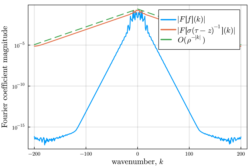
(a) $t^{*}=1+0.05i$

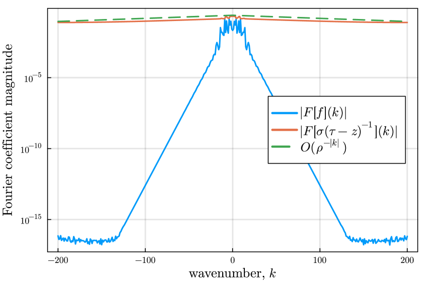
(b) $t^{*}=1+0.005i$

Figure 1: Example results for the Cauchy integral on the starfish geometry and density from section 3.2, for two different $t^{*}$. The Fourier coefficients of the integrand in (3) decay approximately as $\rho^{-|k|}$, where $\rho=e^{|\operatorname{Im}t_{0}|}$, which gets very slow as $z\to\Gamma$. On the other hand, the coefficients of the regularized function $f$ in (9) decay with a rate that changes little as $z\to\Gamma$.

A weakness of the method is that in order to find $t^{*}$, one must evaluate the analytic continuation of $\gamma$ using a truncated Fourier series, which naturally is most accurate close to $\Gamma$. For $z$ far away from $\Gamma$ the rootfinding process will struggle, and the accuracy of SSQ can deteriorate. However, this happens at ranges where the base trapezoidal rule is sufficiently accurate.

Remark 1

The reader may note that one could in fact apply a variant of the Helsing-Ojala quadrature directly to (3). First solve interpolation problem

$$\sum_{k=-K}^{K}c_{k}\tau_{i}^{k}=\sigma_{i},\quad i=0,\dots,N-1,$$ (19)

where $\tau_{i}=\gamma(t_{i})$ and $\sigma_{i}=\gamma(t_{i})$. Then evaluate the layer potential as

$$I_{1}(z)=\sum_{k=-K}^{K}c_{k}\oint_{\Gamma}\frac{\tau^{k}\operatorname{d\!}\tau}{\tau-z},$$ (20)

where the integrals can be exactly evaluated using residue calculus, just as is done above for the unit circle. This will in fact work perfectly fine for some geometries (the unit circle in particular), but the interpolation problem can be severely ill-conditioned in a way that is hard to control, since it depends on the geometry itself. This could potentially be investigated further, but that is deemed beyond the scope of this work.

2.2 Higher order integrals

For higher order integrals ($m>1$), we have

$$I_{m}(z) =\oint_{\Gamma}\frac{\sigma\operatorname{d\!}\tau}{\left(\tau-z\right)^{m}}=\int_{0}^{2\pi}\frac{\sigma(t)\gamma^{\prime}(t)\operatorname{d\!}t}{(\gamma(t)-z)^{m}},\quad m\in\mathbb{Z}^{+}.$$ (21)

Evaluating this integral with SSQ is completely analogous to the case when $m=1$, with the difference that we instead regularize with $(e^{it}-e^{it^{*}})^{m}$, such that

$$f(t,t^{*})=\sigma(t)\gamma^{\prime}(t)\left(\frac{e^{it}-e^{it^{*}}}{\gamma(t)-\gamma(t^{*})}\right)^{m}.$$ (22)

We then need expressions for the integrals

$$p_{k}^{m}(t^{*})=\frac{1}{i}\oint_{S}\frac{\xi^{k-1}\operatorname{d\!}\xi}{\left(\xi-\zeta\right)^{m}}.$$ (23)

Evaluating the residues in the same way as for the $m=1$ case, we get the general expression for integer $m\geq 1$,

$$p_{k}(t^{*})=2\pi\frac{\prod_{j=1}^{m-1}(k-j)}{(m-1)!}e^{i(k-m)t^{*}}\begin{cases}1,&\text{if }\operatorname{Im}t^{*}>0\text{ and }k\geq m,\\ -1,&\text{if }\operatorname{Im}t^{*}<0\text{ and }k\leq 0,\\ 0,&\text{otherwise}.\end{cases}$$ (24)

2.3 Log kernel

Consider now the log integral, also known as the Laplace single-layer potential, for a real-valued density $\sigma$,

$$I_{L}(z) =\oint_{\Gamma}\sigma\log|\tau-z|\>|\operatorname{d\!}\tau|$$ (25)

$$=\int_{0}^{2\pi}\underbrace{\sigma(t)|\gamma^{\prime}|}_{f(t)}\log|\gamma(t)-z|\operatorname{d\!}t,$$ (26)

where $f$ is assumed to be a smooth function. Proceeding in a similar fashion as before, we find $t^{*}$ and separate the integral as

$$I_{L}(z)=\int_{0}^{2\pi}f(t)\left(\log|\gamma(t)-z|-\log|e^{it}-e^{it^{*}}|\right)\operatorname{d\!}t+\int_{0}^{2\pi}f(t)\log|e^{it}-e^{it^{*}}|\operatorname{d\!}t.$$ (27)

The first integral is now regularized, and can be evaluated using the trapezoidal rule. The second integral we rewrite using a truncated Fourier series and the relation $\log|r|=\operatorname{Re}\log r$, such that we can evaluate it using SSQ,

$$\int_{0}^{2\pi}f(t)\log|e^{it}-e^{it^{*}}|\operatorname{d\!}t\approx\operatorname{Re}\sum_{k=-N/2}^{N/2}\hat{f}_{k}\underbrace{\int_{0}^{2\pi}e^{ikt}\log(e^{ikt}-e^{ikt^{*}})\operatorname{d\!}t}_{q_{k}(t^{*})}=\bm{\hat{f}}\cdot\bm{q}.$$ (28)

Just as with $p_{k}$, the integrals $q_{k}$ can be transformed into integrals on the unit circle,

$$q_{k}(t^{*})=\frac{1}{i}\int_{S}\xi^{k-1}\log(\xi-\zeta)\operatorname{d\!}\xi.$$ (29)

Note that this is not necessarily a closed contour integral, as there is a branch cut in the complex logarithm that needs to be taken into account. We will now show to evaluate $q_{k}(t^{*})$ depending on the sign of $\operatorname{Im}t^{*}$.

2.3.1 $\operatorname{Im}t^{*}<0$

Beginning with the case $|\zeta|>1$ (or $\operatorname{Im}t^{*}<0$), we note that $\xi-\zeta\neq 0$ on the entire unit disc. We can therefore choose the branch cut of the complex logarithm such that it never intersects the unit circle. This choice allows us to evaluate the integral in (29) as a contour integral on the unit circle, with a possible pole of order $1-k$ at the origin,

$$\frac{1}{2\pi i}\oint_{S}\xi^{k-1}\log(\xi-\zeta)\operatorname{d\!}\xi=\operatorname{Res}\left[\xi^{k-1}\log(\xi-\zeta),0\right]=\begin{cases}\zeta^{k}/k&\text{ if }k<0,\\ \log(-\zeta)&\text{ if }k=0,\\ 0&\text{ if }k>0.\end{cases}$$ (30)

Since $\hat{f}_{0}\in\mathbb{R}$, we only need the real part of $q_{k}$ at $k=0$. We then have that $\bm{q}$ is for $\operatorname{Im}t^{*}<0$ computed as

$$q_{k}(t^{*})=2\pi\begin{cases}\frac{1}{k}e^{ikt^{*}}&\text{ if }k<0,\\ -\operatorname{Im}t^{*}&\text{ if }k=0,\\ 0&\text{ if }k>0.\end{cases}$$ (31)

2.3.2 $\operatorname{Im}t^{*}>0$

We are now left with the case $|\zeta|<1$ (or $\operatorname{Im}t^{*}>0$). Here, $\xi-\zeta=0$ at at point on the unit disk, so the integral of $\log(\xi-\zeta)$ on the unit circle must intersect the branch cut in the $\xi$ plane going from $\zeta$ to infinity. We choose the branch cut such that it passes through the point $\xi=1$. We define $1^{+}$ and $1^{-}$ to be the limits approaching $1$ from above and below in the plane, such that

$$\log(1^{-}-\zeta)=\log(1^{+}-\zeta)+2\pi i.$$ (32)

Then the integral on the unit circle $S$ is,

$$q_{k}(t^{*})=\frac{1}{i}\int_{1^{+}}^{1^{-}}\xi^{k-1}\log(\xi-\zeta)\operatorname{d\!}\xi.$$ (33)

In order to evaluate this, we let $C$ be the closed contour following the unit circle from $1^{+}$ to $1^{-}$, then going from $1^{-}$ to $\zeta$ on the negative side of the branch cut, and then going from $\zeta$ to $1^{+}$ on the positive side of the branch cut,

$$\oint_{C}=\int_{1^{+}}^{1^{-}}+\int_{1^{-}}^{\zeta}+\int_{\zeta}^{1^{+}}.$$ (34)

The integrand is analytic inside $C$, except for a pole of order $1-k$ at the origin when $k\leq 0$, with residue given by (30). The integrals along the branch cut are

$$\int_{1^{-}}^{\zeta}+\int_{\zeta}^{1^{+}} =\int_{1}^{\zeta}\xi^{k-1}\left(\log(\xi-\zeta)+2\pi i\right)\operatorname{d\!}\xi+\int_{\zeta}^{1}\xi^{k-1}\log(\xi-\zeta)\operatorname{d\!}\xi$$ (35)

$$=2\pi i\begin{cases}\log(\zeta)&\text{ if }k=0,\\ (\zeta^{k}-1)/k&\text{ otherwise}.\end{cases}$$ (36)

Combining the results, and just as before keeping only the real part of the $k=0$ integral, we arrive at the final results for $\operatorname{Im}t^{*}>0$,

$$q_{k}(t^{*})=\frac{2\pi}{k}\begin{cases}1&\text{ if }k<0,\\ 0&\text{ if }k=0,\\ (1-e^{ikt^{*}})&\text{ if }k>0.\end{cases}$$ (37)

3 Experiments

In order to demonstrate the method outlined above, we here report experimental results for the by now well-known “starfish” geometry $\gamma(t)=(1+0.3\cos 5t)e^{it}$. The method has been implemented in Julia, and is available online as open source together with the scripts that produce the numerical in this manuscript.

3.1 Laplace double layer potential

As a first demonstration, we reuse the Laplace test problem from [1]. That is, we evaluate the solution to the Laplace equation $\Delta u=0$ in the domain bounded by $\Gamma$, with boundary condition $u=u_{e}(z)=\log\mathinner{\!\left\lvert 3+3i-z\right\rvert}$. The solution to this problem can be represented using the Laplace double layer potential (DLP) $u(z)=\operatorname{Im}I_{1}(z)$, which leads to a second-kind integral equation in the real-valued density $\sigma$. Once this integral equation is solved, the layer potential $u(z)$ can be evaluated in the domain using quadrature, and compared to the exact solution $u_{e}(z)$.

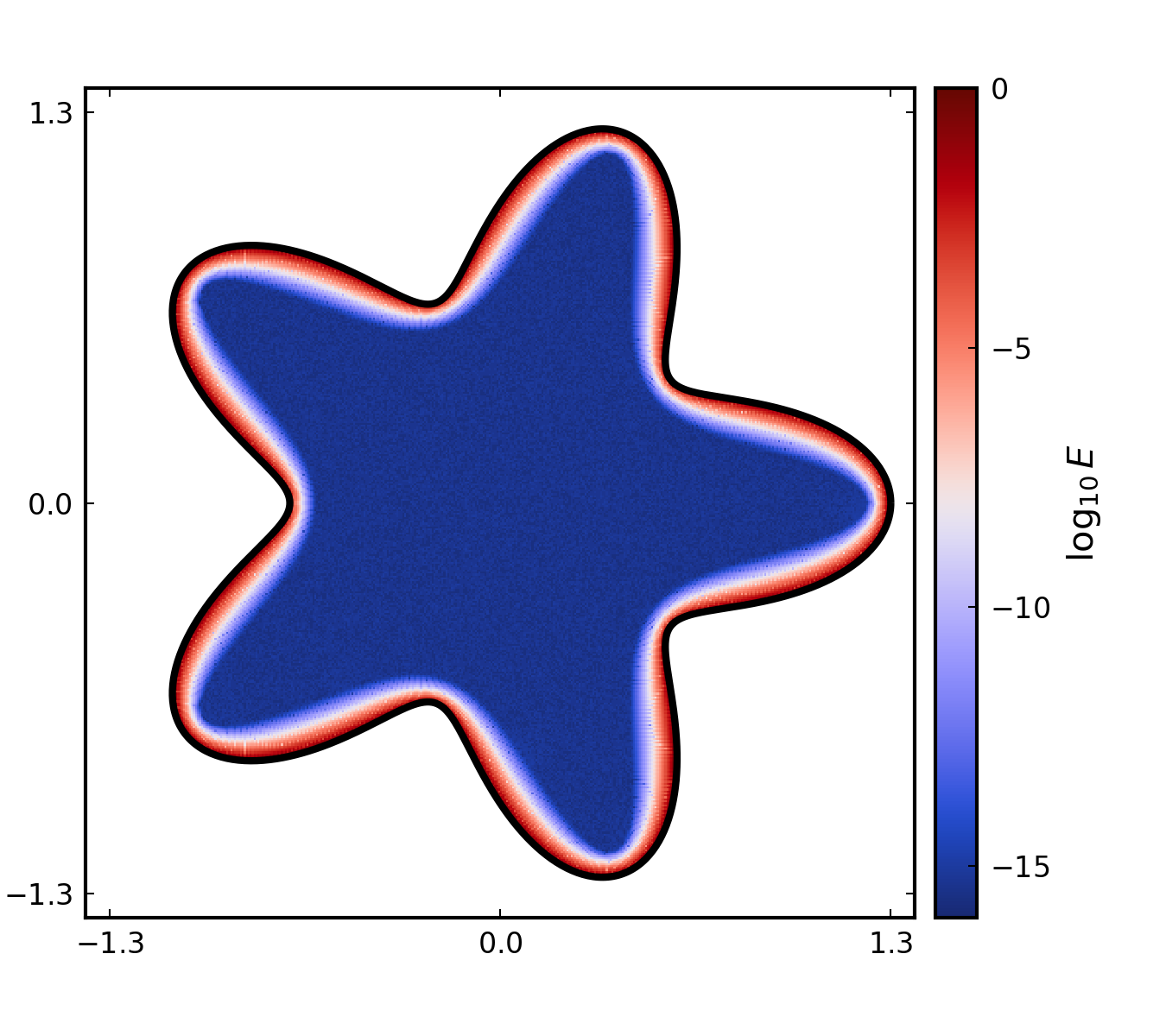
(a) Trapezoidal rule, $E_{\max}=\mathcal{O}(1)$

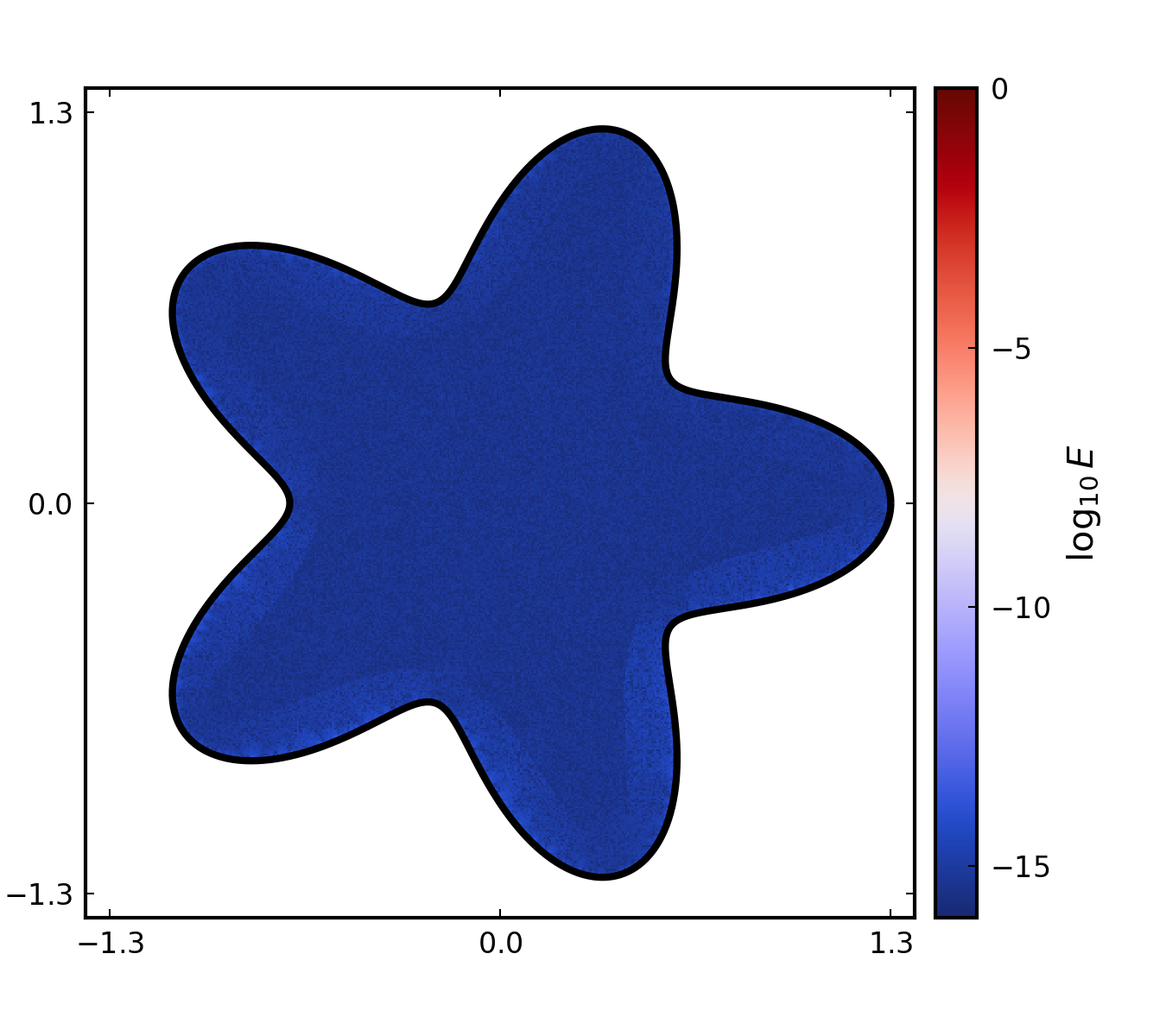
(b) SSQ, $E_{\max}=7\cdot 10^{-13}$

Figure 2: Error in the Laplace double layer potential on a domain with $N=400$ points on the boundary, comparison between the trapezoidal rule and SSQ.

In fig. 2 we show results for the Laplace DLP when $\Gamma$ is discretized using $N=400$ points that are equidistant in the parametrization $t$. The layer potential is evaluated using the trapezoidal rule on a $400\times 400$ grid inside the domain, but for points close to the boundary we also evaluate using SSQ and compare the results. As expected, evaluation using the trapezoidal rule leads to $\mathcal{O}(1)$ errors near the boundary, while SSQ is accurate at all points where it is used. However, full machine precision accuracy is not recovered; the maximum error in SSQ close to the boundary is $\mathcal{O}(10^{-13})$.

3.2 Convergence

For a more systematic investigation of the method, we create the following setup. Let $\Gamma$ be the starfish domain from the previous section, and discretize it using $N$ points. We then create 100 evaluation points as $z=\gamma(t^{*})$, where $\operatorname{Re}t^{*}\in[0,2\pi)$ and $\operatorname{Im}t^{*}=d$. In order to test points both interior and exterior to $\Gamma$, we use $d=\{\pm 0.01,\pm 0.02,\pm 0.04\}$. For a range of $N$, we then compute the integrals $I_{L},I_{1},I_{2},I_{3}$ using both trapezoidal and singularity swap quadrature, and for each $N$ save the maximum error across all $z$. The density $\sigma$ and reference solution used are:

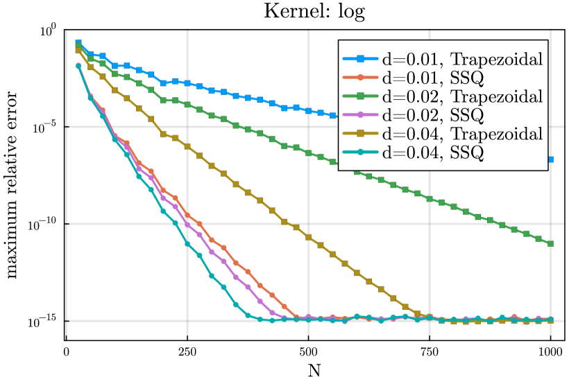
(a)

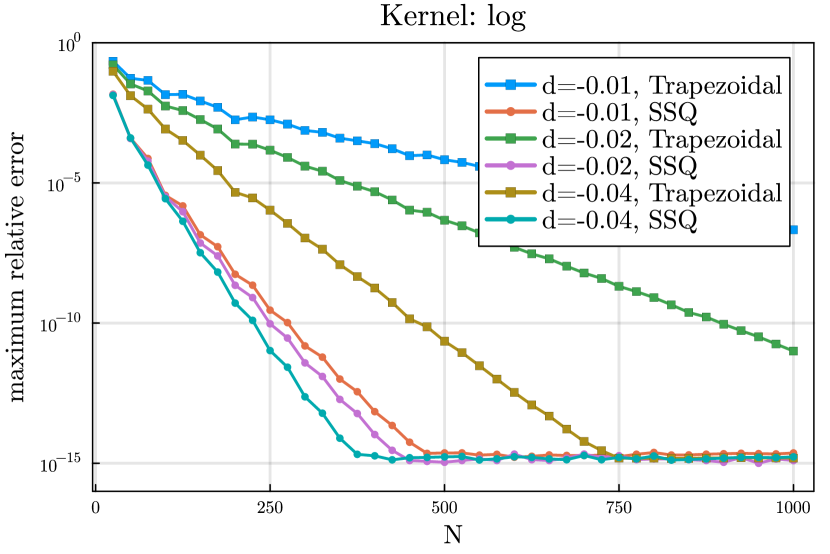
(b)

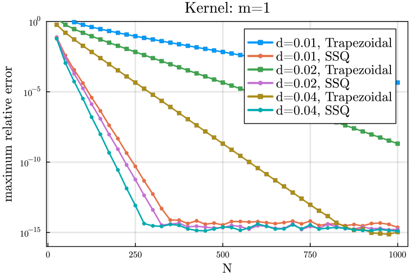
(c)

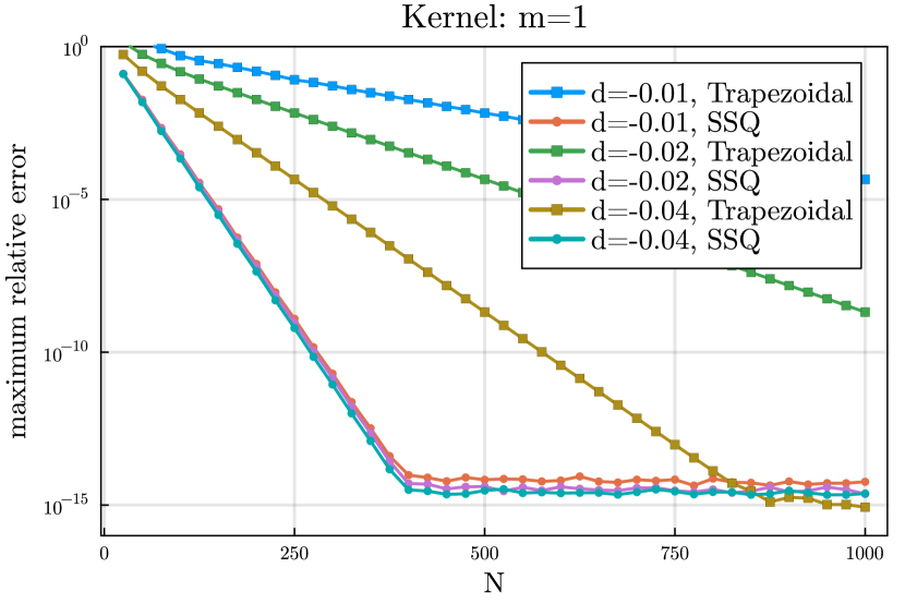
(d)

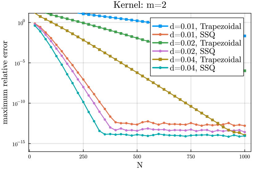
(e)

(f)

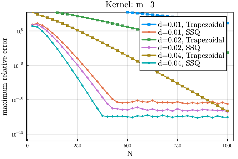
(g)

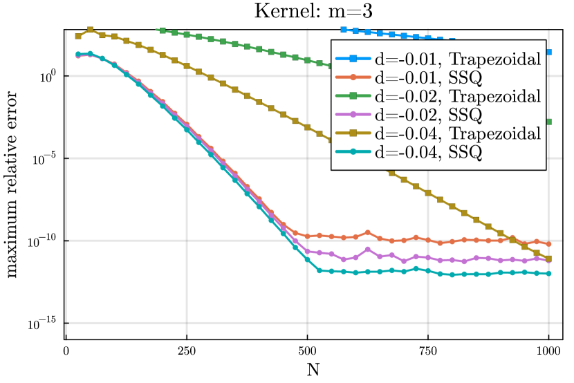
(h)

Figure 3: Convergence of the trapezoidal rule and SSQ for the log kernel and $m=1,2,3$, measured as the maximum error on a set of target points such that $\operatorname{Im}t^{*}=d$. Left column shows interior points, right column shows exterior points.

• For $I_{L}$ we use the $\sigma(t)=g_{1}(t)g_{2}(t)$ and compute the reference solution using adaptive Gauss-Kronrod quadrature.

• For $I_{m}$ and interior points ($\operatorname{Im}t^{*}>0$) we use $\sigma(\tau)=\tau^{3}+\tau$, with reference solution $I_{m}(z)=2\pi i\sigma^{(m)}(z)/(m-1)!$.

• For $I_{m}$ and exterior points ($\operatorname{Im}t^{*}<0$) we use $\sigma(\tau)=\tau^{-1}$, with reference solution $I_{m}(z)=2\pi iz^{-m}$.

The results of this investigation are shown in fig. 3. As expected, the convergence rate of the trapezoidal rule depends strongly on the distance to the boundary, which is not the case for SSQ. There appears to be a weak dependence on the rate for interior points, but that could be an effect of the chosen test problem. More concerning is that lowest attainable error appears to increase for smaller $d$ when $m>1$. It is unclear what causes this effect, although in experiments there appears to be an upper bound to the error growth.

4 Conclusions

We have extended the singularity swap quadrature (SSQ, [1]) method to closed 2D curves discretized using the trapezoidal rule. This extension builds on the simple observation that interpolatory quadrature can be used on a periodic integrand if the problem is first swapped to the unit circle. The method relies on representing quantities as Fourier expansions, and as a consquence the domintaing cost of the method is that of applying the fast Fourier transform (FFT).

The method is accurate, exponentially convergent, and relatively simple to implement (and we provide source code). The fact that the cost is $\mathcal{O}(N\log N)$ per target point makes the method unfeasible for large problems, but that is a consequence of the underlying trapezoidal rule being global (and exponentially convergent). For maximum efficiency, composite Gauss-Legendre quadrature with the original SSQ likely remains the better option.

In the original SSQ paper, it was shown that the method can be applied to line integrals in 3D by finding the singularity preimage through analytic continuation of the squared-distance function. The same technique can be applied to the present method, for closed curves in three dimensions. What remains is analytical evaluation of the integrals of the interpolatory quadrature. This is straightforward for the logarithmic kernel, but the integrals corresponding to power-law kernels are more challenging. Deriving expressions for these is currently work in progress.

Acknowledgements

The key contributions of this work were made with support from the Knut and Alice Wallenberg Foundation, under grant no. 2016.0410.

References

- af Klinteberg and Barnett [2020] L. af Klinteberg and A. H. Barnett. Accurate quadrature of nearly singular line integrals in two and three dimensions by singularity swapping. BIT Numer. Math., 2020. doi:10.1007/s10543-020-00820-5.
- af Klinteberg et al. [2022] L. af Klinteberg, C. Sorgentone, and A. K. Tornberg. Quadrature error estimates for layer potentials evaluated near curved surfaces in three dimensions. Comput. Math. Appl., 111:1–19, 2022. doi:10.1016/j.camwa.2022.02.001.
- Barnett et al. [2015] A. Barnett, B. Wu, and S. Veerapaneni. Spectrally Accurate Quadratures for Evaluation of Layer Potentials Close to the Boundary for the 2D Stokes and Laplace Equations. SIAM J. Sci. Comput., 37(4):B519–B542, 2015. doi:10.1137/140990826.
- Barnett [2014] A. H. Barnett. Evaluation of Layer Potentials Close to the Boundary for Laplace and Helmholtz Problems on Analytic Planar Domains. SIAM J. Sci. Comput., 36(2):A427–A451, 2014. doi:10.1137/120900253.
- Beale and Lai [2001] J. T. Beale and M.-C. Lai. A Method for Computing Nearly Singular Integrals. SIAM J. Numer. Anal., 38(6):1902–1925, 2001. doi:10.1137/S0036142999362845.
- Carvalho et al. [2018] C. Carvalho, S. Khatri, and A. D. Kim. Asymptotic analysis for close evaluation of layer potentials. J. Comput. Phys., 355:327–341, 2018. doi:10.1016/j.jcp.2017.11.015.
- Helsing and Ojala [2008] J. Helsing and R. Ojala. On the evaluation of layer potentials close to their sources. J. Comput. Phys., 227(5):2899–2921, 2008. doi:10.1016/j.jcp.2007.11.024.
- Nitsche [2022] M. Nitsche. Corrected trapezoidal rule for near-singular integrals in axi-symmetric Stokes flow. Adv. Comput. Math., 48(5):57, 2022. doi:10.1007/s10444-022-09973-z.
- Trefethen and Weideman [2014] L. N. Trefethen and J. A. C. Weideman. The Exponentially Convergent Trapezoidal Rule. SIAM Rev., 56(3):385–458, 2014. doi:10.1137/130932132.