Glocal Energy-based Learning for Few-Shot Open-Set Recognition

Abstract

Few-shot open-set recognition (FSOR) is a challenging task of great practical value. It aims to categorize a sample to one of the pre-defined, closed-set classes illustrated by few examples while being able to reject the sample from unknown classes. In this work, we approach the FSOR task by proposing a novel energy-based hybrid model. The model is composed of two branches, where a classification branch learns a metric to classify a sample to one of closed-set classes and the energy branch explicitly estimates the open-set probability. To achieve holistic detection of open-set samples, our model leverages both class-wise and pixel-wise features to learn a glocal energy-based score, in which a global energy score is learned using the class-wise features, while a local energy score is learned using the pixel-wise features. The model is enforced to assign large energy scores to samples that are deviated from the few-shot examples in either the class-wise features or the pixel-wise features, and to assign small energy scores otherwise. Experiments on three standard FSOR datasets show the superior performance of our model.

1 Introduction

In recent years, deep learning has flourished in various fields with the ever-increasing scale of the training data under the closed-world learning settings, i.e., the training and test sets share exactly the same set of classes. However, such settings often do not hold in many real applications. This is because 1) it is difficult or costly to obtain a large amount of labeled data, and 2) models deployed in open-world environments need to constantly deal with samples from unknown classes. For example, in the application of deep learning for diagnosing rare diseases, the number of samples is limited. In this case, the model is prone to over-fitting, resulting in a significant degradation in performance. Further, there can be unknown variants of those diseases due to our limited understanding of the diseases. Thus, the models are required to perform the classification accurately for the classes illustrated by limited samples, while at the same time detecting the samples from unknown classes. The latter ability is important, especially for healthcare or safety-critical applications, e.g., to alert the unknown cases for human investigation in the disease diagnosis example, or to request human intervention for handling unknown objects in autonomous driving.

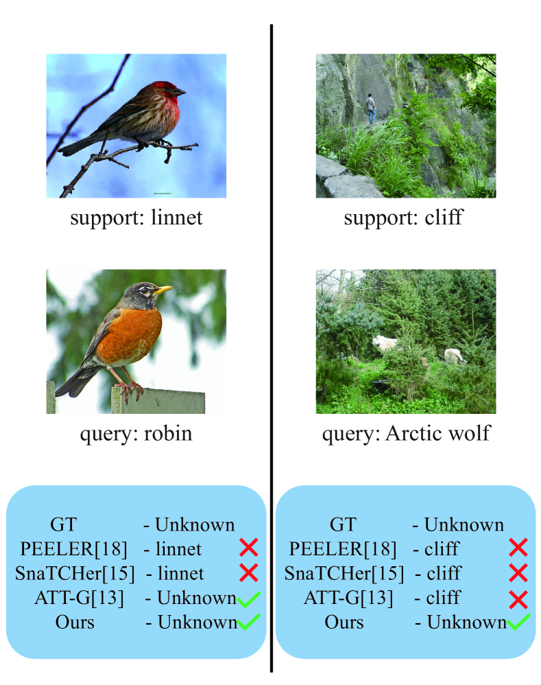
Figure 1: Two typical errors with existing methods. Our method can detect unknown open-set samples that are similar to the closed-set samples in either the global class level or the local feature level.

Few shot learning [32, 36, 16, 23, 35, 28] (FSL) and open set recognition [29, 30, 7, 3, 9, 22] (OSR) are two techniques dedicated to solve these two problems, respectively. FSL methods are trained to achieve a good generalization ability on the new task with only a few training samples. But FSL approaches are developed under a closed-set setting. It lacks the ability to distinguish the classes unseen during training. The goal of OSR is, on the other hand, to recognize open-set samples while maintaining the classification ability of closed-set samples. However, its classification ability is often built upon the availability of a large number of training samples. Thus, OSR approaches fail to work effectively when only a few training samples are available.

Few-shot open-set recognition (FSOR), which combines the FSL and OSR problems, is a largely under-explored area. FSOR requires the model to utilize only a few training samples to effectively achieve the ability of both closed-set classification and open-set recognition. Existing FSOR methods [15, 13, 6] are based on the prototype network [32], which performs classification by measuring the distance between the prototype of each class and the query embedding feature of a sample. They improve the original closed-set classifier in recognizing open-set samples by learning an additional open-set class using pseudo open-set samples. However, only the class-wise information of the sample is considered, and the pixel-wise spatial information of the sample is ignored. As shown in Figure 1, these methods fail to distinguish open-set samples from closed-set class samples that share similar global semantic appearances. Further, the optimization objectives of FSL and OSR are different from each other. Thus, training using only an open-set classifier can limit the performance of these models.

To solve the above problems, we propose a novel FSOR method, called Glocal Energy-based Learning (GEL). Different from previous methods, GEL consists of two classification components: one for closed-set classification and one for open-set recognition. Specifically, in addition to use the class-wise features to classify closed-set samples in the closed-set classifier, GEL leverages both class-wise and pixel-wise features to learn a new energy-based open-set classifier, in which a global energy score is learned using the class-wise features while a local energy score is learned using the pixel-wise features. GEL is enforced to assign large energy scores to samples that are deviated from the few-shot examples in either the class-wise features or the pixel-wise features, and to assign small energy scores otherwise. In doing so, GEL can detect unknown class samples that are deviated from the known classes in either high-level abstractions or fine-grained appearances, as shown in Figure 1.

In summary, this work makes the following three main contributions:

• We propose a novel FSOR framework that learns glocal open scores for detecting unknown samples from the class-wise (global) and pixel-wise (local) scales.

• We further propose a novel energy-based FSOR model, dubbed GEL, that learns glocal energy-based open scores based on the class-wise and pixel-wise similarities of query samples to the support set.

• Through extensive experiments on three widely-used datasets, we show that GEL outperforms state-of-the-art competing methods and achieves state-of-the-art results on these benchmarks.

2 Related Work

2.1 Few-Shot Learning

Few-shot learning has been widely studied in computer vision. The approaches of FSL can be divided into two categories: meta-learning based approaches and transfer learning approaches. There are three subcategory of meta-learning based approaches. The first is metric-based approaches [32, 36, 16] which learn a distance function through training samples. Another subcategory is optimization-based approaches [23, 33, 27, 35, 14, 1, 40, 43], it learns a priors to optimize the model on limited training examples without overfitting. The last subcategory is model-based approaches [28, 5, 20, 21, 19]. Different from the previous two approaches, model-based approaches use support samples to generate model weights adapted to new task. Another category of FSL is transfer learning [38, 34, 8]. Transfer learning improve the performance in a new task through transferring knowledge from a learned related task.

2.2 Open-Set Recognition

Open-set recognition is a more realistic scenario because it is usually difficult to include all classes when training a classifier. OSR requires the classifier to classify not only known classes, but also unknown classes. There are two mainstream approaches for OSR. One is discriminative model. It includes traditional machine learning methods [29, 30, 42, 2, 25] and deep neural network methods [7, 3, 11, 31]. The former is popular before deep neural network rise. It usually adapt the limitation of traditional methods that training and testing data are from the same distribution for OSR. The latter uses the powerful representation ability of deep neural network to solve OSR through network architecture design. The other mainstream approach is generative model [9, 22, 39, 10]. It usually use generative adversarial network or Dirichlet Process to generate unknown samples as training samples to improve model performance.

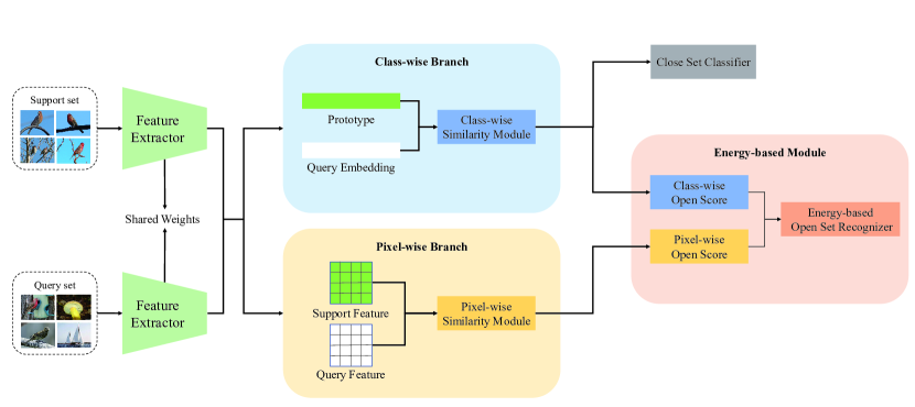
Figure 2: An overview of our model GEL. Our model mainly consists of three parts: a class-wise branch, which is used to calculate the similarity between embeddings for closed-set classification and open-set recognition, a pixel-wise branch, which is used to calculate the similarity between feature maps for open-set recognition, and an energy-based module, which performs open-set recognition on query samples by feeding the similarities from the two branches to learn glocal energy scores.

2.3 Few-Shot Open-Set Recognition

Compared with FSL and OSR, there are few studies focused on few shot open-set recognition, which mainly include the following three methods. The first is the loss function based method. Based on the original distance-based classifier, PEELER [18] proposes an open-set loss to improve the accuracy of open-set recognition by increasing the entropy of classification results of open-set samples. The second method is based on transformation consistency. SnaTCHer [15] adds each query embedding replacement to the prototype set, and determines whether the query sample is an open-set sample by measuring the difference between the sets before and after transformation. By measuring the difference before and after the change of the set, the unknown class distribution estimation problem is transformed into a relative feature transformation problem which is unrelated to the unknown class samples. The third method is to add an extra open-set class. TANE [13] and RFDNet [6] expands the closed-set classifier by using a generative network to obtain an additional open-set classes prototype from closed-set prototype. They then add the prototype to the original classifier to enable it to perform both closed-set classification and open-set recognition. By adding an additional category to classify the query sample, the measuring based on the entropy or the threshold of the sample is changed to dynamic classification.

3 Preliminary

The goal of the FSOR is to identify open-set samples while maintaining the classification capability of closed-set with only a few data samples. In particular, for a N-way K-shot Q-query sampled from dataset $\mathcal{D}$, the FSOR task can be presented as: $\mathcal{T}=\{\mathcal{S},\mathcal{Q}_{k},\mathcal{Q}_{u}\}$, where $\mathcal{S}=\{x_{i},y_{i}\}_{i=1}^{|\mathcal{S}|}$ and $\mathcal{Q}_{k}=\{x_{i},y_{i}\}_{i=1}^{|\mathcal{Q}_{k}|}$ are support set and known query set, respectively. The label $y$ corresponding to the image $x$ in these two sets are from closed-set categories $\mathcal{C}_{k}$. Different from FSL, $\mathcal{Q}_{u}=\{x_{i},y_{i}\}_{i=1}^{|\mathcal{Q}_{u}|}$ is a set of query samples from unknown classes $\mathcal{C}_{u}$, and $\mathcal{C}_{k}\cap\mathcal{C}_{u}=\varnothing$.

4 Method

We will describe our approach in detail in this section. First, we will give an overview of our proposed method GEL, then introduce our proposed pixel-wise similarity module, and finally introduce our energy-based open-set recognizer.

4.1 Overview

Figure 2 shows the overall architecture of our model. Following previous FSOR methods [18, 15, 13, 6], we use metric-based meta-learning architecture. First, the embedding and feature maps of the support and query samples are obtained through a shared feature extractor $\mathcal{F}_{\theta}$, where $\theta$ denots the shared parameters. For each input support sample $x_{i}^{\mathcal{S}}$, we obtain its embedding $e_{i}^{\mathcal{S}}$ and feature map $f_{i}^{\mathcal{S}}$ by $e_{i}^{\mathcal{S}}=avg\ pooling(\mathcal{F}_{\theta}(x_{i}^{\mathcal{S}}))$ and $f_{i}^{\mathcal{S}}=\mathcal{F}_{\theta}(x_{i}^{\mathcal{S}})$, respectively. For each query sample $x_{i}^{\mathcal{Q}}$, we use the same way to obtain its query embedding $e_{i}^{\mathcal{Q}}$ and feature map $f_{i}^{\mathcal{Q}}$. The channel dimension of them is $dim$.

For the class-wise branch, we first compute the prototype $p$ for each of the N classes by averaging over support embeddings. Particularly, for a class $n$, its prototype $p_{n}$ is calculated from all support embedding of class $n$ by

$$p_{n}=\frac{1}{K}\sum_{i=1}^{K}\mathcal{F}_{\theta}(e_{n,i}^{\mathcal{S}}).$$ (1)

Then we follow [15] to simply use a self-attention module to enhance the class prototypes. For the matrix $P\in\mathbbm{R}^{N\times dim}$ composed by all prototypes, the enhanced prototype matrix $P^{*}$ is calculated as follows

$$P^{q}=PW^{q},\ P^{k}=PW^{k},\ P^{v}=PW^{v},$$ (2)

$$P^{*}=softmax(\frac{P^{q}{P^{k}}^{T}}{\sqrt{d_{P^{k}}}})P^{v},$$ (3)

where $W^{q},W^{k},W^{v}\in\mathbbm{R}^{dim\times dim}$ are coefficient matrices that linearly map the prototype matrix, and $d_{P^{k}}$ is the channel dimension of $P^{k}$.

Finally, we obtain the class-wise similarity $s_{c}$ by measuring the distance between the query embedding and the enhanced class prototype:

$$s_{c}^{i,n}=-distance(e_{i}^{\mathcal{Q}},p_{n}^{*}),$$ (4)

where $s_{c}^{i,n}$ is the class-wise similarity between $x_{i}^{\mathcal{Q}}$ and the enhanced prototype of class $n$, $distance(\cdot,\cdot)$ is a distance function. We use Euclidean distance by default, because we found it performed best through experiments.

In closed-set classification, only the class-wise similarity $s_{c}$ is used to classify query samples in $\mathcal{Q}_{k}$ through a softmax function:

$$p(y=n|x_{i})=\frac{e^{s_{c}^{i,n}}}{\sum_{j\in\mathcal{C}_{k}}e^{s_{c}^{i,j}}}.$$ (5)

Then we use cross entropy loss to optimize the model:

$$L_{c}=\frac{1}{NQ}\sum_{i=1}^{NQ}\sum_{j\in\mathcal{C}_{k}}\mathbbm{1}_{x_{i}=j}log(p(y=n|x_{i})),$$ (6)

where $\mathbbm{1}_{condition}$ is an indicative function, which is one if the condition is met, and zero otherwise, and$p(y=n|x_{i})$ is the probability that the label of sample $x_{i}$ is class $n$.

Our model extends this popular FSL approach to FSOR by using both class-wise similarity and pixel-wise similarity to learn a global energy-based open-set recognizer. We will detail our proposed module in the next two subsections.

4.2 Pixel-wise Similarity Module

In order to have a holistic recognition of open-set samples, in addition to the class-wise information, we also consider the pixel-wise information. As shown in Figure 1, our idea is based on the following two key points. First, if the class of open-set samples is similar to that of closed-set samples, the distance between their embeddings would be so small, so it is difficult to distinguish them. However, human beings usually distinguish them by a certain key part. Secondly, if the large background of the open-set and closed-set samples are similar, it is often difficult to extract the class information only by using the embeddings. But humans can pick up the key parts directly from the background. Inspired by these two observations, we propose a novel pixel-wise similarity module. First, we use the same method as the class-wise branch to obtain the feature map for each class. Formally, for a class $n$, its feature map $f_{n}$ is defined as

$$f_{n}=\frac{\sum_{i=1}^{K}f_{i}}{K}.$$ (7)

In order to keep the distance between pixel-wise features and class-wise features within the same scale convenient for fusion and reduce the amount of computation, we first apply a scale calibration module to all feature maps. Specifically, we use a point-wise convolution to halve the channel dimension of the feature map, followed by a Batch Normalization layer and a PReLU activation function:

$$f^{*}=PReLU(BN(Conv(f))).$$ (8)

Finally, for each pixel of the class feature map and query, we calculate the pixel-level similarity using cosine similarity. And for each query pixel, we consider the top-k nearest neighbours in class feature map pixels and calculate the summation for the top-k similarity scores to form a robust fine-grained metric for open-set learning:

$$s_{f}^{i,n}=\sum_{pixel}topk(\frac{f_{i}^{*}\cdot f_{n}}{||f_{i}^{*}||\cdot||f_{n}||})/T,$$ (9)

where $f_{n}\in\mathbbm{R}^{\frac{dim}{2}\times m^{2}}$ and $f_{i}^{*}\in\mathbbm{R}^{m^{2}\times\frac{dim}{2}}$ are the feature map of class $n$ and query sample $x_{i}$, respectively; $m$ is the spatial dimension of feature map; $||\cdot||$ is applied to the fourth dimension; $\sum_{pixel}$ sum over all the remaining pixels after calculating $topk$; and $T$ is a temperature coefficient.

Remark. Attention mechanism is also a common method to focus on local information in the deep learning approach, but in the few-shot open-set recognition task, this can easily result in over-fitting because of the lack of samples. Our proposed pixel-wise similarity module has only a few learnable parameters in the scale calibration module, well alleviating the over-fitting issue.

4.3 Energy-based Module

The existing FSOR methods often use cross-entropy-based classifiers, because for closed-set classification, entropy-based classifiers can often achieve better results by classifying the samples using prediction probability. However, for our dual-branch architecture, we have a dedicated energy-based open-set recognizer to classify open-set samples. By using energy-based models, we eliminate the complexity in the process of normalization the probability distribution in entropy-based classification. Thus, they are more suitable for the FSOR task.

Our energy-based module integrates the class-wise and pixel-wise similarity results from the two branches and then feed them to train into glocal energy-based few-shot open-set recognizer.

4.3.1 Margin-based Energy Loss

We then feed these glocal energy scores to an energy loss function to optimize our model. The model is trained to ensure that the energy is large when the samples are from unknown classes, and it is small otherwise. To achieve this goal, we use a margin-based energy loss to optimize the model. Particularly, for a query sample $x_{i}$, its energy loss is calculated by

$$L_{e}^{x_{i}}=\left\{\begin{array}[]{cl}max(0,E^{x_{i}}-M_{k})&\mathbbm{1}_{y_{i}\in\mathcal{C}_{k}}\\ max(E^{x_{i}}-M_{u},0)&\mathbbm{1}_{y_{i}\in\mathcal{C}_{u}},\\ \end{array}\right.$$ (10)

where $M_{k}$ and $M_{u}$ are the margins of closed-set and open-set samples, respectively. $\mathcal{C}_{u}$ are pseudo open set samples, consisting of $Q$ samples of each class from $N$ classes that do not overlap with the closed-set classes $\mathcal{C}_{k}$. Both $\mathcal{C}_{u}$ and $\mathcal{C}_{k}$ are part of the training set. The energy loss for the task is

$$L_{e}=\sum_{\mathcal{Q}_{k}\cup\mathcal{Q}_{u}}L_{e}^{x_{i}}.$$ (11)

Thus, the total loss of our GEL model is

$$L=L_{c}+\lambda L_{e},$$ (12)

where $\lambda$ is a hyperparameter that balances the two losses.

4.3.2 Glocal Energy Function

For a query sample $x_{i}$, its class-wise (global) similarity to class $n$ is $s_{c}^{i,n}$, while its pixel-wise (local) similarity is $s_{f}^{i,n}$. We first use these two similarities to respectively define the global and local energy through the energy function as follows:

$$E_{c}=-log\sum_{n\in\mathcal{C}_{k}}(e^{s_{c}^{i,n}}),$$ (13)

$$E_{f}=-log\sum_{n\in\mathcal{C}_{k}}(e^{s_{f}^{i,n}}).$$ (14)

Since we have used the scale calibration module in the pixel-wise similarity module to adjust the scale of similarity score, the final glocal open-set energy of the sample can be obtained by a simple addition:

$$E=E_{c}+E_{f}.$$ (15)

Other combination methods are evaluated and compared in our ablation study in Sec. 6.3.

5 Experiments

5.1 Datasets

We use miniImageNet [37], tieredImageNet [24] and CIFAR-FS [4] to evaluate the performance of the model. MiniImageNet contains a total of 60,000 images of size $84\times 84$ in 100 categories, including 600 samples in each category. The category for training, validation and testing set is 64, 16, and 20, respectively. TieredImageNet is a larger dataset. It contains a total of 779,165 images of size $84\times 84$ in 608 categories, including 351 for training, 97 for validation and 160 for testing. Both of them are the subsets of ILSVRC-12 [26]. CIFAR-FS is the subsets of CIFAR100 [17]. It contains a total of 60,000 images of size $32\times 32$ in 100 categories. The categories are divided in the same way as miniImageNet.

5.2 Metrics

To measure the effectiveness of the FSOR methods, following  [18, 15, 13, 6], we use ACC and AUROC as the metrics. ACC is used to measure the classification accuracy of the closed-set samples. It can be calculated by dividing the number of correctly classified samples in $\mathcal{Q}_{k}$ by the number of samples in $\mathcal{Q}_{k}$. AUROC is used to measure the accuracy of open-set recognition. It is the area under the ROC curve for open-set recognition of all query samples $\mathcal{Q}_{k}\cup\mathcal{Q}_{u}$. A larger ACC or AUROC indicates better performance.

We also calculate F1 Score, FPR95 and AUPR for the open-set recognition in our ablation study. F1 Score is the harmonic average of precision and recall. FPR95 is short for FPR@TPR95, which is the false positive rate when the true positive rate is 95%. The smaller the FPR95 is, the better the model is. AUPR is the area under the PR curve. Compared to AUROC on balanced datasets, AUPR is a more indicative metric in highly unbalanced datasets.

Dataset	Methods	Publication	1-shot		5-shot
			ACC	AUROC	ACC	AUROC
miniImageNet	ProtoNet [32]	NIPS2017	$64.01\pm 0.88$	$51.81\pm 0.93$	$80.09\pm 0.58$	$60.39\pm 0.92$
	FEAT [41]	CVPR2020	$67.02\pm 0.85$	$57.01\pm 0.84$	$82.02\pm 0.53$	$63.18\pm 0.78$
	PEELER [18]	CVPR2020	$58.31\pm 0.58$	$61.66\pm 0.62$	$75.08\pm 0.72$	$69.85\pm 0.70$
	PEELER* [18]		$65.86\pm 0.85$	$60.57\pm 0.83$	$80.61\pm 0.59$	$67.35\pm 0.80$
	SnaTCHer-F [15]	CVPR2021	$67.02\pm 0.85$	$68.27\pm 0.96$	$82.02\pm 0.53$	$77.42\pm 0.73$
	SnaTCHer-T [15]		$66.60\pm 0.80$	$70.17\pm 0.88$	$81.77\pm 0.53$	$76.66\pm 0.78$
	SnaTCHer-L [15]		$67.60\pm 0.83$	$69.40\pm 0.92$	$82.36\pm 0.58$	$76.15\pm 0.83$
	ATT [13]	CVPR2022	$67.64\pm 0.81$	$71.35\pm 0.68$	$82.31\pm 0.49$	$79.85\pm 0.58$
	ATT-G [13]		$68.11\pm 0.81$	$72.41\pm 0.72$	$83.12\pm 0.48$	$79.85\pm 0.57$
	RFDNet* [6]	TMM2022	$66.23\pm 0.80$	$71.37\pm 0.80$	$82.44\pm 0.54$	$80.31\pm 0.59$
	Ours		$68.26\pm 0.85$	$73.70\pm 0.82$	$83.05\pm 0.55$	$82.29\pm 0.60$
tieredImageNet	ProtoNet [32]	NIPS2017	$68.26\pm 0.96$	$60.73\pm 0.80$	$83.40\pm 0.65$	$64.96\pm 0.83$
	FEAT [41]	CVPR2020	$70.52\pm 0.96$	$63.54\pm 0.76$	$84.74\pm 0.69$	$70.74\pm 0.75$
	PEELER* [18]	CVPR2020	$69.51\pm 0.92$	$65.20\pm 0.76$	$84.10\pm 0.66$	$73.27\pm 0.71$
	SnaTCHer-F [15]	CVPR2021	$70.52\pm 0.96$	$74.28\pm 0.80$	$84.74\pm 0.69$	$82.02\pm 0.64$
	SnaTCHer-T [15]		$70.45\pm 0.95$	$74.84\pm 0.79$	$84.42\pm 0.68$	$82.03\pm 0.66$
	SnaTCHer-L [15]		$70.85\pm 0.99$	$74.95\pm 0.83$	$85.23\pm 0.64$	$80.81\pm 0.68$
	ATT [13]	CVPR2022	$69.34\pm 0.95$	$72.74\pm 0.78$	$83.82\pm 0.63$	$78.66\pm 0.65$
	ATT-G [13]		$70.58\pm 0.93$	$73.43\pm 0.78$	$85.38\pm 0.61$	$81.64\pm 0.63$
	RFDNet* [6]	TMM2022	$66.84\pm 0.89$	$72.68\pm 0.76$	$82.64\pm 0.63$	$80.63\pm 0.63$
	Ours		$70.50\pm 0.93$	$75.86\pm 0.81$	$84.60\pm 0.65$	$81.95\pm 0.72$
CIFAR-FS	FEAT* [41]	CVPR2020	$70.89\pm 0.89$	$74.83\pm 0.79$	$83.96\pm 0.64$	$82.88\pm 0.67$
	PEELER* [18]	CVPR2020	$71.47\pm 0.67$	$71.28\pm 0.57$	$85.46\pm 0.47$	$75.97\pm 0.33$
	SnaTCHer-F* [15]	CVPR2021	$75.09\pm 0.87$	$78.15\pm 0.77$	$87.18\pm 0.62$	$85.81\pm 0.64$
	ATT-G [13]	CVPR2022	$72.43\pm 0.65$	$76.72\pm 0.59$	$86.52\pm 0.49$	$84.64\pm 0.38$
	RFDNet* [6]	TMM2022	$73.83\pm 0.92$	$75.35\pm 0.77$	$85.12\pm 0.74$	$84.40\pm 0.64$
	Ours		$76.77\pm 0.88$	$78.67\pm 0.80$	$86.74\pm 0.66$	$86.56\pm 0.59$
	Ours w/o Pix		$76.67\pm 0.90$	$79.43\pm 0.72$	$87.63\pm 0.62$	$86.84\pm 0.58$

Table 1: 5-way 1-shot and 5-shot results on miniImageNet, tieredImageNet and CIFAR-FS. We calculated ACC and AUROC of each model. * denotes implementation on ResNet-12.

5.3 Implementation Details

Following previous FSOR methods [18, 15, 13, 6], we use ResNet-12 [12] as the feature extractor of our network. By default, it uses 16x drop sampling of the images and generates a feature map with 640 channel dimensions before pooling layer. We use a widely-used FSL method FEAT [41] to pre-train the feature extractor. For the setting of hyperparameters, we set $T$ in Eq. 9 to the k value in the $topk$ function. Because of the scale calibration module, we simply set $M_{k}$ to -1 and $M_{u}$ to 1 in Eq. 10. The loss weight $\lambda$ in Eq. 12 is set to 0.1.

During the training phase, we use the SGD optimizer to train the model for over 60,000 tasks. The learning rate is set to 0.0001 for feature extractor and 0.001 for the other initially and decayed by the factor of 10 for every 12,000 tasks. We then select the model with the best results through the validation set for testing. For data augmentation, following [13], in the pre-training phase, RandomCrop, ColorJitter, RandomHorizontalFilp, and RandomRotate are used; and only RandomCrop and RandomHorizontalFilp are used for meta-training and testing.

For a N-way K-shot FSOR task, we following previous FSOR methods [18, 15, 13, 6] to select 2N classes in the dataset, half of which are known classes and the other are unknown classes. For known classes, we sample K images for each class as support set and another 15 images as known query set. For each unknown classes, we only sample 15 images as unknown query set. During the testing phase, the first 75 query samples with the highest open-set scores (i.e., the energy score in Eq. 15) are taken as open-set samples to calculate the open-set recognition metrics.

6 Results

6.1 Comparison Methods

Our method GEL is compared with the FSL approach ProtoNet [32] and FEAT [41]. Since most of the existing FSOR methods are based on the metric-based FSL method, we compare the most representative method ProtoNet and the most competitive method FEAT. In order to evaluate the open-set recognition performance, we input the open-set samples into their closed-set classifier and recognize them by thresholding the entropy. We also make a comparison with existing SOTA few-shot open-set approaches PEELER [18], SnaTCHer [15], ATT [13] and RFDNet [6]. For fair comparison, since the original PEELER and RFDNet used ResNet-18 as the feature extractor, we re-implemented a version based on ResNet-12, named PEELER* and RFDNet*. We use the source code of FEAT and SnaTCHer-F from github to do the experiment on the CIFAR-FS. In addition, SEMAN-G [13] uses additional word embedding information, which we do not have, and so its results cannot be fairly compared to GEL and the other methods.

6.2 FSOR Results

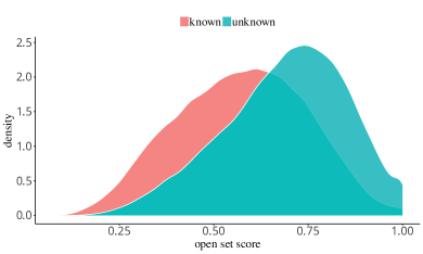
(a) SnaTCHer-F, IoU=0.57

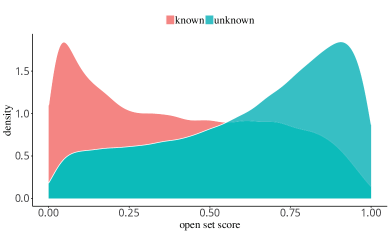
(b) ATT-G, IoU=0.53

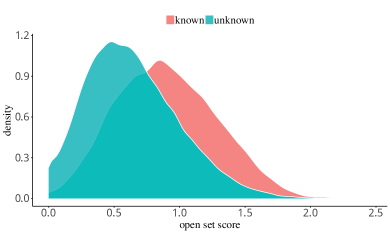
(c) RFDNet, IoU=0.55

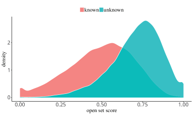
(d) Ours, IoU=0.47

Figure 3: Density map for normalized score histogram on miniImageNet 5-way 1-shot. By sampling 600 tasks for each method, we first make the open set score non-negative, then use the maximum value in each task for normalization. We can see that our method can better distinguish between known and unknown samples.

Table 1 shows the results of our method GEL compared to the others on three datasets and two different shots. As can be observed, although the FSL method has a good performance in closed-set classification, its open-set recognition is poor. Compared to the previous FSOR methods, our method is substantially more effective: it obtains the best open-set recognition results (i.e., AUROC) across the three datasets in the 1-shot setting, and it is the best performer in AUROC on two datasets in the 5-shot setting, while at the same time maintaining the very competitive closed-set classification accuracy. It is worth mentioning that compared with the other two datasets, the image resolution of CIFAR-FS is very small. After the feature extraction, the spatial dimension of the feature map is only $2\times 2$, which makes it difficult for the pixel branch to learn useful local information. Therefore, we also give the results without using the pixel branch on this dataset (i.e., Ours w/o Pix). It can be seen from the results that when the image size is small, only using the energy-based open-set recognizer can often achieve better results.

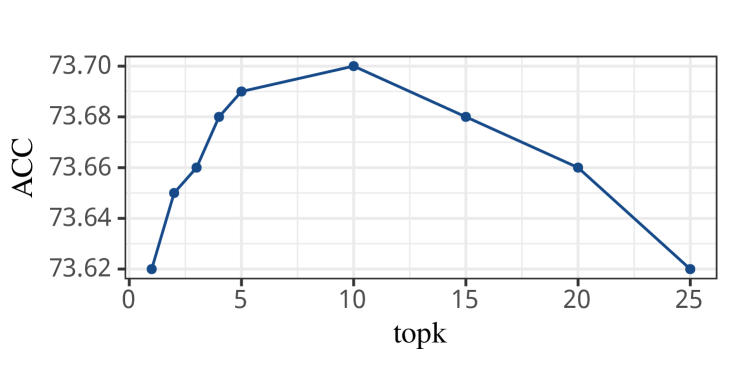
(a) Ablation study of the value of $topk$ on miniImageNet under 5-way 1-shot setting.

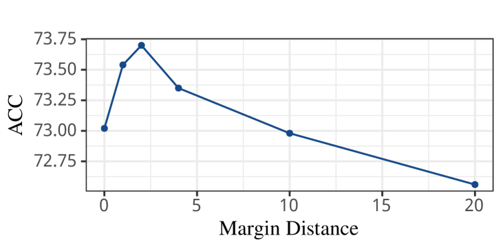
(b) Ablation study of margin distance on miniImageNet under 5-way 1-shot setting.

Figure 4: Ablation study of two hyperparameters on mimiImageNet under 5-way 1-shot setting .

To further demonstrate the power of our model, we compare the open-set score distribution for known and unknown samples in miniImageNet 5-way 1-shot in 600 tasks. Figure 3 compares the normalized score histogram of open-set scores between SnaTCHer-F, ATT-G, RFDNet and Our method. Since the open-set score (energy for ours and entropy for others) of known samples in our method is usually negative, we first subtract the minimum value in each task if it is negative. Then we normalized the open-set scores of all samples obtained from each task by dividing it by the maximum value, and subsequently calculate the density. We use the intersection over union (IoU) to quantitatively evaluate the overlap between the known and unknown distribution (the smaller the better), i.e. OSR capability. As can be seen from the figure, the overlap of two different color areas of our method is smaller. In other words, our method can better distinguish the known and unknown samples.

6.3 Ablation Study

Table 2 presents the ablation study results of the 5-way 1-shot experiments on two different datasets for our three proposed modules. In addition to ACC and AUROC, we also calculate F1 Score, FPR95 and AUPR of open-set recognition. From the results, it can be seen that all the three proposed modules we propose can improve the performance of open-set recognition while keeping the closed-set classification ability almost unchanged.

Method	Dataset	ACC$\uparrow$	AUROC$\uparrow$	F1 Score$\uparrow$	FPR95$\downarrow$	AUPR$\uparrow$
Baseline	miniImageNet	$68.53\pm 0.78$	$69.85\pm 0.87$	$65.06\pm 0.69$	$79.35\pm 1.45$	$70.53\pm 0.83$
+ Energy Loss		$68.14\pm 0.78$	$71.97\pm 0.83$	$65.92\pm 0.69$	$77.88\pm 1.34$	$71.96\pm 0.83$
+ Pixel wise		$68.40\pm 0.86$	$72.49\pm 0.76$	$67.38\pm 0.69$	$74.99\pm 1.35$	$73.28\pm 0.85$
+ Combine score		$68.26\pm 0.85$	$73.70\pm 0.82$	$67.72\pm 0.70$	$74.10\pm 1.38$	$73.80\pm 0.87$
Baseline	tieredImageNet	$70.55\pm 0.93$	$71.66\pm 0.82$	$67.02\pm 0.63$	$74.66\pm 1.40$	$71.01\pm 0.83$
+ Energy Loss		$70.60\pm 0.94$	$73.57\pm 0.84$	$67.90\pm 0.61$	$72.60\pm 1.46$	$73.48\pm 0.86$
+ Pixel wise		$70.39\pm 0.96$	$74.06\pm 0.73$	$67.90\pm 0.61$	$71.72\pm 1.32$	$73.10\pm 0.75$
+ Combine score		$70.50\pm 0.93$	$75.86\pm 0.81$	$69.44\pm 0.68$	$70.22\pm 1.47$	$75.78\pm 0.80$

Table 2: Ablation study of three modules proposed in GEL. We report the 5-way 1-shot results on both miniImageNet and tieredImageNet to demonstrate the effectiveness of our modules.

Method	ACC	AUROC
Delay Combine	$68.39\pm 0.86$	$73.17\pm 0.83$
Ahead Combine	$68.26\pm 0.85$	$73.70\pm 0.82$

(a) miniImageNet 5-way 1-shot

Method	ACC	AUROC
Delay Combine	$83.00\pm 0.55$	$80.67\pm 0.65$
Ahead Combine	$83.05\pm 0.55$	$82.29\pm 0.60$

(b) miniImageNet 5-way 5-shot

Table 3: Ablation study of glocal energy score combination of the class-wise branch and pixel-wise branch on miniImageNet under 5-way 1-shot and 5-shot setting.

In addition, we also evaluate the effect of k in Eq. 9 and distance between $M_{k}$ and $M_{u}$ in Eq. 10 on the performance. As shown in Figure 4 (a), for the selection of different k values in our method, the variation range of AUROC is only 0.08, indicating that our method is robust to the selection of this hyperparameters. And for the choice of margin distance, in the experiment, we calculate the size of the two margins with zero as the center. As shown in Figure 4 (b), the margin distances is greater than zero, and a smaller margin often enables the model to perform better.

For the calculation of open-set scores, in addition to combining the energy calculation as we did, called ahead combine below, the energy can be calculated only for the pixel branch at first, and then combined with the class-wise similarity, which is denoted as delay combine. We perform the ablation study on miniImageNet with the above two methods. As can be seen in Table 3, the ahead combine method improves the performance of open-set recognition, especially when the shot is large.

Method	ACC	AUROC
Fixed value	$83.05\pm 0.55$	$82.29\pm 0.60$
Learnable	$83.08\pm 0.56$	$81.37\pm 0.64$
Task-adaptive	$83.00\pm 0.56$	$81.34\pm 0.62$

(a) miniImageNet 5-way 5-shot

Method	ACC	AUROC
Fixed value	$84.60\pm 0.65$	$81.95\pm 0.72$
Learnable	$84.84\pm 0.65$	$80.86\pm 0.70$
Task-adaptive	$84.79\pm 0.66$	$80.49\pm 0.72$

(b) tieredImageNet 5-way 5-shot

Table 4: Ablation study of combination coefficients between class-wise energy and pixel-wise energy on miniImageNet and tieredImageNet under 5-way 5-shot setting.

We also conduct an ablation study on the combination coefficient between class-wise energy and pixel-wise energy in Eq. 15. Three methods are used: fixed value, learnable coefficient, and task-adaptive learnable coefficient on miniImageNet 5-way 5-shot. For method with a fixed value, we simply set the weight of the two branches to one. For the method with learnable coefficient, we use two learnable parameters with an initial value of one to learn the coefficients, and for the method with task-adaptive learnable coefficient, we use a linear layer to generate two coefficients from the prototypes in each task. As shown in Table 4, although learnable coefficient methods can slightly improve the classification ability of the closed-set samples, the fixed coefficient method can greatly improve the recognition ability of detecting open-set samples.

7 Conclusion

In this paper, we explore the under-explored problem, few-shot open-set recognition (FSOR). To have holistic detection of open-set samples, we propose a novel FSOR method, called Glocal Energy-based Learning (GEL). GEL improves the open-set recognition capability in few-shot settings by fusing global and local information. By combining the similarities from the class-wise and pixel-wise branches, GEL learns glocal energy scores, in which large energy scores are enforced for samples that are deviated from the few-shot examples in either the class-wise features or the pixel-wise features, and small energy scores are enforced otherwise. In doing so, GEL can detect open-set samples that are similar to the closed-set samples in either the global class level or the local feature level, while the existing methods fail to do. Extensive experiments on multiple datasets demonstrate the effectiveness of our proposed method.

8 Acknowledgments

This work was supported in part by the National Natural Science Foundation of Chain under Grant 62101454, Grant 62071387, and Grant U19B2037; in part by the Fundamental Research Funds for the Central Universities; and in part by the Shenzhen Fundamental Research Program under Grant JCYJ20190806160210899. P. Wang’s participation was in part supported by Australian Research Council Discovery Projects (DP220101784). G. Pang was supported in part by the Singapore Ministry of Education (MoE) Academic Research Fund (AcRF) Tier 1 grant (21SISSMU031).

References

- [1] Antreas Antoniou, Harrison Edwards, and Amos Storkey. How to train your maml. arXiv preprint arXiv:1810.09502, 2018.
- [2] Abhijit Bendale and Terrance Boult. Towards open world recognition. In Proceedings of the IEEE conference on computer vision and pattern recognition, pages 1893–1902, 2015.
- [3] Abhijit Bendale and Terrance E Boult. Towards open set deep networks. In Proceedings of the IEEE conference on computer vision and pattern recognition, pages 1563–1572, 2016.
- [4] Luca Bertinetto, Joao F Henriques, Philip HS Torr, and Andrea Vedaldi. Meta-learning with differentiable closed-form solvers. arXiv preprint arXiv:1805.08136, 2018.
- [5] Qi Cai, Yingwei Pan, Ting Yao, Chenggang Yan, and Tao Mei. Memory matching networks for one-shot image recognition. In Proceedings of the IEEE conference on computer vision and pattern recognition, pages 4080–4088, 2018.
- [6] Shule Deng, Jin-Gang Yu, Zihao Wu, Hongxia Gao, Yansheng Li, and Yang Yang. Learning relative feature displacement for few-shot open-set recognition. IEEE Transactions on Multimedia, 2022.
- [7] Akshay Raj Dhamija, Manuel Günther, and Terrance Boult. Reducing network agnostophobia. Advances in Neural Information Processing Systems, 31, 2018.
- [8] Guneet S Dhillon, Pratik Chaudhari, Avinash Ravichandran, and Stefano Soatto. A baseline for few-shot image classification. arXiv preprint arXiv:1909.02729, 2019.
- [9] ZongYuan Ge, Sergey Demyanov, Zetao Chen, and Rahil Garnavi. Generative openmax for multi-class open set classification. arXiv preprint arXiv:1707.07418, 2017.
- [10] Chuanxing Geng and Songcan Chen. Collective decision for open set recognition. IEEE Transactions on Knowledge and Data Engineering, 34(1):192–204, 2020.
- [11] Mehadi Hassen and Philip K Chan. Learning a neural-network-based representation for open set recognition. In Proceedings of the 2020 SIAM International Conference on Data Mining, pages 154–162. SIAM, 2020.
- [12] Kaiming He, Xiangyu Zhang, Shaoqing Ren, and Jian Sun. Deep residual learning for image recognition. In Proceedings of the IEEE conference on computer vision and pattern recognition, pages 770–778, 2016.
- [13] Shiyuan Huang, Jiawei Ma, Guangxing Han, and Shih-Fu Chang. Task-adaptive negative envision for few-shot open-set recognition. In Proceedings of the IEEE/CVF Conference on Computer Vision and Pattern Recognition, pages 7171–7180, 2022.
- [14] Muhammad Abdullah Jamal and Guo-Jun Qi. Task agnostic meta-learning for few-shot learning. In Proceedings of the IEEE/CVF Conference on Computer Vision and Pattern Recognition, pages 11719–11727, 2019.
- [15] Minki Jeong, Seokeon Choi, and Changick Kim. Few-shot open-set recognition by transformation consistency. In Proceedings of the IEEE/CVF Conference on Computer Vision and Pattern Recognition, pages 12566–12575, 2021.
- [16] Gregory Koch, Richard Zemel, Ruslan Salakhutdinov, et al. Siamese neural networks for one-shot image recognition. In ICML deep learning workshop, volume 2, page 0. Lille, 2015.
- [17] Alex Krizhevsky, Vinod Nair, and Geoffrey Hinton. Cifar-10 (canadian institute for advanced research). URL http://www. cs. toronto. edu/kriz/cifar. html, 5(4):1, 2010.
- [18] Bo Liu, Hao Kang, Haoxiang Li, Gang Hua, and Nuno Vasconcelos. Few-shot open-set recognition using meta-learning. In Proceedings of the IEEE/CVF Conference on Computer Vision and Pattern Recognition, pages 8798–8807, 2020.
- [19] Nikhil Mishra, Mostafa Rohaninejad, Xi Chen, and Pieter Abbeel. A simple neural attentive meta-learner. arXiv preprint arXiv:1707.03141, 2017.
- [20] Tsendsuren Munkhdalai and Hong Yu. Meta networks. In International Conference on Machine Learning, pages 2554–2563. PMLR, 2017.
- [21] Tsendsuren Munkhdalai, Xingdi Yuan, Soroush Mehri, and Adam Trischler. Rapid adaptation with conditionally shifted neurons. In International Conference on Machine Learning, pages 3664–3673. PMLR, 2018.
- [22] Lawrence Neal, Matthew Olson, Xiaoli Fern, Weng-Keen Wong, and Fuxin Li. Open set learning with counterfactual images. In Proceedings of the European Conference on Computer Vision (ECCV), pages 613–628, 2018.
- [23] Sachin Ravi and Hugo Larochelle. Optimization as a model for few-shot learning. 2016.
- [24] Mengye Ren, Eleni Triantafillou, Sachin Ravi, Jake Snell, Kevin Swersky, Joshua B Tenenbaum, Hugo Larochelle, and Richard S Zemel. Meta-learning for semi-supervised few-shot classification. arXiv preprint arXiv:1803.00676, 2018.
- [25] Ethan M Rudd, Lalit P Jain, Walter J Scheirer, and Terrance E Boult. The extreme value machine. IEEE transactions on pattern analysis and machine intelligence, 40(3):762–768, 2017.
- [26] Olga Russakovsky, Jia Deng, Hao Su, Jonathan Krause, Sanjeev Satheesh, Sean Ma, Zhiheng Huang, Andrej Karpathy, Aditya Khosla, Michael Bernstein, et al. Imagenet large scale visual recognition challenge. International journal of computer vision, 115(3):211–252, 2015.
- [27] Andrei A Rusu, Dushyant Rao, Jakub Sygnowski, Oriol Vinyals, Razvan Pascanu, Simon Osindero, and Raia Hadsell. Meta-learning with latent embedding optimization. arXiv preprint arXiv:1807.05960, 2018.
- [28] Adam Santoro, Sergey Bartunov, Matthew Botvinick, Daan Wierstra, and Timothy Lillicrap. Meta-learning with memory-augmented neural networks. In International conference on machine learning, pages 1842–1850. PMLR, 2016.
- [29] Walter J Scheirer, Anderson de Rezende Rocha, Archana Sapkota, and Terrance E Boult. Toward open set recognition. IEEE transactions on pattern analysis and machine intelligence, 35(7):1757–1772, 2012.
- [30] Walter J Scheirer, Lalit P Jain, and Terrance E Boult. Probability models for open set recognition. IEEE transactions on pattern analysis and machine intelligence, 36(11):2317–2324, 2014.
- [31] Lei Shu, Hu Xu, and Bing Liu. Doc: Deep open classification of text documents. arXiv preprint arXiv:1709.08716, 2017.
- [32] Jake Snell, Kevin Swersky, and Richard Zemel. Prototypical networks for few-shot learning. Advances in neural information processing systems, 30, 2017.
- [33] Qianru Sun, Yaoyao Liu, Tat-Seng Chua, and Bernt Schiele. Meta-transfer learning for few-shot learning. In Proceedings of the IEEE/CVF Conference on Computer Vision and Pattern Recognition, pages 403–412, 2019.
- [34] Yonglong Tian, Yue Wang, Dilip Krishnan, Joshua B Tenenbaum, and Phillip Isola. Rethinking few-shot image classification: a good embedding is all you need? In European Conference on Computer Vision, pages 266–282. Springer, 2020.
- [35] Eleni Triantafillou, Tyler Zhu, Vincent Dumoulin, Pascal Lamblin, Utku Evci, Kelvin Xu, Ross Goroshin, Carles Gelada, Kevin Swersky, Pierre-Antoine Manzagol, et al. Meta-dataset: A dataset of datasets for learning to learn from few examples. arXiv preprint arXiv:1903.03096, 2019.
- [36] Oriol Vinyals, Charles Blundell, Timothy Lillicrap, Daan Wierstra, et al. Matching networks for one shot learning. Advances in neural information processing systems, 29, 2016.
- [37] Oriol Vinyals, Charles Blundell, Timothy Lillicrap, Daan Wierstra, et al. Matching networks for one shot learning. Advances in neural information processing systems, 29, 2016.
- [38] Yan Wang, Wei-Lun Chao, Kilian Q Weinberger, and Laurens van der Maaten. Simpleshot: Revisiting nearest-neighbor classification for few-shot learning. arXiv preprint arXiv:1911.04623, 2019.
- [39] Yang Yang, Chunping Hou, Yue Lang, Dai Guan, Danyang Huang, and Jinchen Xu. Open-set human activity recognition based on micro-doppler signatures. Pattern Recognition, 85:60–69, 2019.
- [40] Huaxiu Yao, Ying Wei, Junzhou Huang, and Zhenhui Li. Hierarchically structured meta-learning. In International Conference on Machine Learning, pages 7045–7054. PMLR, 2019.
- [41] Han-Jia Ye, Hexiang Hu, De-Chuan Zhan, and Fei Sha. Few-shot learning via embedding adaptation with set-to-set functions. In Proceedings of the IEEE/CVF Conference on Computer Vision and Pattern Recognition, pages 8808–8817, 2020.
- [42] He Zhang and Vishal M Patel. Sparse representation-based open set recognition. IEEE transactions on pattern analysis and machine intelligence, 39(8):1690–1696, 2016.
- [43] Luisa Zintgraf, Kyriacos Shiarli, Vitaly Kurin, Katja Hofmann, and Shimon Whiteson. Fast context adaptation via meta-learning. In International Conference on Machine Learning, pages 7693–7702. PMLR, 2019.