Stochastic Approximation for Nonlinear Discrete Stochastic Control: Finite-Sample Bounds

Abstract

We consider a nonlinear discrete stochastic control system, and our goal is to design a feedback control policy in order to lead the system to a prespecified state. We adopt a stochastic approximation viewpoint of this problem. It is known that by solving the corresponding continuous-time deterministic system, and using the resulting feedback control policy, one ensures almost sure convergence to the prespecified state in the discrete system. In this paper, we adopt such a control mechanism and provide its finite-sample convergence bounds whenever a Lyapunov function is known for the continuous system. In particular, we consider four cases based on whether the Lyapunov function for the continuous system gives exponential or sub-exponential rates and based on whether it is smooth or not. We provide the finite-time bounds in all cases. Our proof relies on constructing a Lyapunov function for the discrete system based on the given Lyapunov function for the continuous system. We do this by appropriately smoothing the given function using the Moreau envelope. We present numerical experiments corresponding to the various cases, which validate the rates we establish.

1 Introduction

In this paper, we consider the problem of controlling a nonlinear discrete stochastic system of the form,

$$x_{k+1}=x_{k}+\alpha_{k}(F(x_{k},u_{k})+w_{k})$$ (1)

where $x_{k}\in\mathbb{R}^{d}$ is the state vector, $u_{k}\in\mathbb{R}^{m}$ is the control, $w_{k}$ is the noise, $F(\cdot,\cdot)$ is in general a nonlinear mapping, and $\alpha_{k}$ is a sequence of step-sizes. The goal is to pick the control sequence $u_{k}$ in order to ensure that the system reaches a pre-specified state $x^{*}$. We will focus on feed-back control strategies of the form $u_{k}=\rho(x_{k})$ for some mapping $\rho:\mathbb{R}^{d}\rightarrow\mathbb{R}^{m}$ to reach the state $x^{*}$. In this paper, we provide finite-time convergence bounds on the error, $\left\lVert x_{k}-x^{*}\right\rVert$ depending on the choice of the step-size sequence $\alpha_{k}$.

Such a problem arises in several control settings such as adaptive regulation [1], [2] with widespread applications such as disturbance rejection in spacecraft systems [3] and frequency regulation in power systems [4]; or selector control with an application in air-fuel control [5]. A special case of our framework (1) is the unforced setting without a $u_{k}$, and in this case, one is interested in the convergence rate to the equilibrium $x^{*}$. A large class of stochastic optimization [6] and reinforcement learning [7] algorithms fit in this framework, and our results immediately apply to this case.

Stochastic recursions of the form (1) are studied under the name of Stochastic Approximation [8], and were first introduced by Robins and Monro [9]. Asymptotic behavior of such recursions is well understood [10, 11, 8] in terms of the behavior of the corresponding continuous-time deterministic control system,

$$\dot{x}=F(x,u)\forall x\in\mathbb{R}^{d}$$ (2)

In particular, it is known that [8] under appropriate assumptions on the system, noise and choice of step-sizes, the almost-sure asymptotic behavior of the discrete-stochastic system (1) is identical to that of the continuous-deterministic system (2). Then, in order to lead the system to state $x^{*}$, one would find the optimal feedback solution $u=\rho(x(t))$ for the continuous system (2) and use the same solution for the discrete system (1). The objective of this paper is to characterize the finite-time convergence error in such an approach.

Naturally, the convergence rate of the discrete system depends on that of the continuous system. The convergence behavior as well as the rate of convergence of the continuous system is usually studied using Lyapunov arguments. In this paper, we characterize the convergence rate of the discrete system (1) based on the properties of the Lyapunov function of the continuous system (2). Suppose that there exists a feedback control policy and the corresponding Lyapunov function $V$ for the continuous system that satisfies

$$\frac{dV}{dt}=\langle\nabla V(x),F(x)\rangle\leq-\gamma V(x)^{c}\forall x\in\mathbb{R}^{d}\text{ for some }\gamma>0,c\geq 1.$$ (3)

The convergence rate of the discrete system was established in the literature (in the context of optimization [6] and reinforcement learning [12]) in the special case when $c=1$ (also known as the global exponential stability [13]) and $V(\cdot)$ is smooth (i.e., has Lipschitz gradients). In contrast, in this paper, we consider the case when the continuous system can either have exponential or sub-exponential rates ($c\geq 1$), while also allowing for non-smooth Lyapunov functions. The main contributions of the paper are as follows.

1.1 Main contributions

Results: We establish finite-time bounds and the following sample complexity results for the SA algorithm for the control problem in (1) based on the properties of the Lyapunov function (3) for the corresponding continuous time system (2) under appropriate assumptions on noise and growth of the Lyapunov function in all four cases.

1. For completeness, we first present the case of exponential stability ($c=1$) and smooth Lyapunov function $V(\cdot)$ which immediately follows from [12]. We show that one needs $O\left(\frac{1}{\varepsilon}\right)$ samples to ensure that the mean square error $\mathbb{E}[\left\lVert x_{k}-x^{*}\right\rVert^{2}]$ is less than $\varepsilon$.

2. In the exponential case ($c=1$) with a non-smooth Lyapunov function, we again establish the same sample complexity.

3. For the sub-exponential case ($c>1$) with a smooth Lyapunov function, we show a sample complexity of $O\left(\frac{1}{\varepsilon^{2c-1}}\right)$.

4. Finally, in the non-smooth sub-exponential case, we establish a sample complexity of $O\left(\frac{1}{\varepsilon^{3d_{a,c}-1}}\right)$ where $a$ is the polynomial growth rate of the Lyapunov function and $d_{a,c}=a(c-1)/2+1$. We believe that this is not optimal, and obtaining tighter results is an open problem.

Methodology: Our key idea is to use the Lyapunov function from the continuous system to study the convergence rate of the discrete system. This works in the case when the Lyapunov function is smooth, even though the rate one obtains in the discrete system is worse than that of the continuous system due to the presence of noise. However, this approach does not work when the Lyapunov function is not smooth. In other words, in the absence of smoothness, one cannot get a handle on the errors between the continuous and discrete systems. So, in the exponential nonsmooth case, we construct a new Lyapunov function obtained by smoothing out the Lyapunov function of the continuous system. We do this by applying the infimal convolution [14] with respect to the $\ell_{2}$ norm square function. This is called the Moreau envelope [15, 7]. Finally, in the nonsmooth subexponential case, naive smoothing does not work, and so, we use a time-varying smoothness parameter to obtain a time-varying Moreau envelope. The use of time-varying Moreau envelopes may be of independent interest.

Numerical Experiments: We empirically validate our results in the latter three cases using three examples: Selector control problem (non-smooth exponentially stable system), Artstein’s circle example (non-smooth sub-exponentially stable system), and a synthetic nonlinear system example for smooth sub-exponentially stable systems.

1.2 Relevant literature

Finding the equilibrium point of stabilizing control problems is essentially a root-finding problem. From this perspective, the equilibrium point finding problems can be solved through the framework of Stochastic Approximation (SA) algorithms, which were first proposed by [9]. The asymptotic convergence of SA methods was analyzed using its associated ordinary differential equations (ODE) [10, 11]. More specifically, it was shown in [8, 16] that under some conditions, the SA algorithm converges almost surely as long as the corresponding ODE is stable. The asymptotic convergence of SA algorithms with Markovian noise has been studied extensively [8, 17]. The convergence of other SA variants such as SA with Markovian noise and multiple time-scale SA was previously explored in [18, 19, 20, 21, 22]. In contrast to asymptotic convergence guarantees in the literature, here we focus on obtaining finite-time bounds which enable us to provide sample complexity bounds.

In order to analyze the stability of dynamical systems, it is common to employ control Lyapunov functions. In particular, one shows that the time derivative of the Lyapunov function is upper bounded by some negative definite function to show asymptotic stability (or some negative constant times the Lyapunov function itself to achieve exponential stability) [23]. In this work, we seek to obtain finite-time analyses for nonlinear systems with a Lyapunov descent condition or some decay conditions. In the context of subgradient optimization, [24] showed that descent properties hold for any function with a Whitney stratifiable graph, covering a wide range of functions in optimization, control and Machine Learning. Indeed, such conditions are found in many settings and applications in control [25, 26, 13], electrical systems [27], robotics [28], diffusion processes [29] and reinforcement learning [30, 31, 32]. In optimization, the Polyak-Lojasiewicz condition [33] establishes that the $\ell_{2}$ norm serves as a Lyapunov function with exponential stability. Previously, [12] established finite-time analysis for nonlinear SA using an exponential dissipativity assumption, which is equivalent to exponential stability condition for the $\ell_{2}$ norm Lyapunov function. However, due to its reliance on the dissipativity assumption, its results are limited to the case of $\ell_{2}$ norm Lyapunov function and exponential stability. In this paper, we generalize the results to the case of subexponential nonlinear nonsmooth Lyapunov functions.

In practice, many control Lyapunov functions are non-smooth [25] since the control inputs are usually measured in discrete time rather than having continuous measurements, such as logical systems [34] or approximate discrete-time models [35]. In addition, discontinuous stabilizing feedback and non-smooth Lyapunov functions are deeply connected [36] as the non-existence of a smooth control Lyapunov function implies the absence of a continuous stabilizing feedback law [25]. The theory of Lyapunov stability for non-smooth systems was developed by [37], where the Clarke generalized gradient [38] was used to complement the lack of gradient as we usually have in the smooth setting. The non-smooth Lyapunov analysis of equilibria is present in the differential inclusions literature [39, 38, 40], with applications in robotics [41] and non-smooth Stochastic Approximation [42]. The work [23] uses the ODE approach to handle the time derivative condition. A special application of non-smooth SA is the switching SA algorithm which is used in networked systems [43]. However, these prior works did not have a finite-time guarantee for the non-smooth stochastic systems.

In order to deal with the non-smoothness of the system, one can attempt smoothing methods to yield a smoothened Lyapunov function. In non-smooth optimization, Moreau envelopes and proximal operators are commonly used [15] to handle the non-smooth component of the objective [14]. Previously, Moreau envelopes have been used as potential functions to analyze the convergence rate of optimization algorithms in non-smooth settings [44]. Specifically, the authors used the norm of the gradient of the Moreau envelope as a measure of progress, which is a proxy for the distance from $0$ to the set of generalized gradients. In the context of SA, [7] was the first to use Moreau envelopes to obtain convergence rates for the non-smooth infinity norms, which is common for the analysis of Reinforcement Learning algorithms. However, the authors relied on the contractive property for analysis, which can be limiting as it excludes a wide range of potential operators without such property and the systems in control settings may not have such properties. The paper [25] used the inf-convolution operator to analyze the stochastic stabilization when a control policy exists. In contrast to these prior works, our interest is to establish finite-time bounds for nonlinear SA algorithms with Lyapunov exponentially decay conditions instead of the contractive assumption for arbitrary norms. Time-varying Moreau envelopes are also used in composite optimization [45]. Besides using Moreau envelopes for smoothing, Nesterov smoothing is another approach for problems with max functions [46] which we will not consider here.

1.3 Paper organization

The paper is organized as follows. Section 2 presents the problem formulation, assumptions and results in all four cases. We present the finite-time convergence bounds and also show that they immediately imply almost sure convergence results. Section 3 presents the proof outline and the key ideas in the proofs. Section 4 presents numerical experiments demonstrating the convergence rate in various examples. Finally, complete proofs of the main results are presented in the Appendix.

2 System model and Main Results

2.1 System model and general assumptions

Consider the following noiseless discrete dynamics:

$$x_{k+1}=x_{k}+\alpha_{k}F(x_{k},u_{k})$$ (4)

where $\mathbb{F}:\mathbb{R}^{d}\rightarrow\mathbb{R}$ be a possibly nonlinear mapping, $x,u\in\mathbb{R}^{d}$ are the state vector and the control vector respectively. Suppose that the control $u$ follows a feed-in control rule $u=\rho(x)$ where $\rho:\mathbb{R}^{d}\rightarrow\mathbb{R}^{m}$, the core of our interests is finding the solution $x^{*}$ to the stationary point equation $F(x,\rho(x))=0$. In control, this is equivalent to finding a control that stabilizes our system given the state.

Now, suppose that we can only obtain the value of $F$ via a noisy oracle $\tilde{F}$ such that for any $x$ it will return $\tilde{F}(x,u)=F(x,u)+w$ where $w$ is the noise (which can be dependent on the state value $x$ and the control $u$).

$$x_{k+1}=x_{k}+\alpha_{k}(F(x_{k},u_{k})+w_{k})$$ (5)

This happens when the control agent tries to obtain environmental inputs via some device, which can be contaminated by noise or device inaccuracies. Let $\mathcal{F}_{k}=\{x_{0},w_{0},...,x_{k-1},w_{k-1},x_{k}\}$ where $\{w_{k}\}$ is a martingale difference sequence with some mild conditions on its variance. We have some assumptions on the noise $w_{k}$ as follows:

Assumption 1.

(Noise assumptions) The noise $w_{k}$ is unbiased, that is for any $k\in\mathbb{Z}^{+}$:

$$\mathbb{E}[w_{k}|\mathcal{F}_{k}]=0$$ (6)

and the noise is square-integrable. That is:

$$\mathbb{E}[\left\lVert w_{k}\right\rVert_{2}^{2}|\mathcal{F}_{k}]\leq A+B\left\lVert x_{k}\right\rVert_{2}^{2}.$$ (7)

In addition to these noise assumptions, we also assume that $F$ is Lipschitz:

Assumption 2.

(Lipschitz assumption of $F$) There exists a positive constant $C$ such that:

$$\left\lVert F(x,u)-F(y,u)\right\rVert_{2}\leq C\left\lVert x-y\right\rVert_{2}$$ (8)

for any $x,y\in\mathbb{R}^{d}$.

In the Stochastic Gradient Descent (SGD) algorithm where $F(x)=-\nabla V(x)$, this assumption is the gradient Lipschitz assumption that is vital to ensure the stability of the algorithm. In addition, this assumption is a much more relaxed assumption than the usual contractive assumption used in [7]. Not having to rely on the contractive property will allow us to apply our results to a wider range of problems rather than just the optimal control problem with time-discounted rewards. From these assumptions, we will proceed to analyze the systems in different settings as follows:

2.2 Stochastic control of smooth exponentially stable systems

First, for completeness, we will consider smooth, exponentially stable systems. This setting is widespread in Stochastic Optimization (which is analogous to the smooth, strongly-convex case [47]) and Reinforcement Learning [12]. To that end, let us assume that we have the following assumptions of $V$:

Assumption 3.

(Exponential stability assumption of the Lyapunov function) Assume that the gradient of $V$ exists everywhere, we have that:

$$\langle\nabla V(x),F(x)\rangle\leq-\gamma V(x)\forall x\in\mathbb{R}^{d}$$ (9)

for some constant $\gamma>0$.

In the Stochastic Gradient Descent (SGD) algorithm, we have that $F(x)=-\nabla V(x)$. Thus, the assumption 3 is equivalent to $\left\lVert\nabla V(x)\right\rVert^{2}\geq\gamma V(x)\forall x\in\mathbb{R}^{d}$, which is the Polyak-Lojasiewicz condition. Combining with the gradient Lipschitz assumption, its convergence results are known [47]. Here, we are considering a more general operator $F$ rather than a gradient of some functions. In addition, in the context of continuous dynamical systems, such conditions imply the global exponential stability of the system, meaning that the system will approach the equilibrium point exponentially fast. This is because the LHS of (9) is somewhat approximating the time derivative of $V$ since $\dot{V}(x)=\langle\nabla V(x),\dot{x}\rangle\approx\langle\nabla V(x),F(x)\rangle$.

Assumption 4.

(Lipschitz gradient assumption) There exists a positive constant $L$ such that:

$$V(y)\leq V(x)+\nabla V(x)^{T}(y-x)+\frac{L\left\lVert x-y\right\rVert^{2}}{2}\forall x,y\in\mathbb{R}^{d}$$ (10)

The gradient Lipschitz assumption is commonly found in optimization literature and is commonly used to obtain a first-order upper bound on the objective function. In addition, this assumption also implies that $V$ is upper-bounded by some quadratic function as well. Indeed, from Assumption 4 we have:

$$V(x)\leq V(x^{*})+\nabla V(x^{*})(x-x^{*})+\frac{L\left\lVert x-x^{*}\right\rVert^{2}}{2}=V(x^{*})+\frac{L\left\lVert x-x^{*}\right\rVert^{2}}{2}\forall x\in\mathbb{R}^{d}$$

hence we have $V$ is upper-bounded by some quadratic function. Thus, we assume that $a=2$ in assumption 7. This gives rise to the following assumption:

Assumption 5.

(Quadratic growth assumption of $V$) There exists positive constants $C_{1},C_{2}$ such that:

$$C_{1}\left\lVert x-x^{*}\right\rVert_{2}^{2}\leq V(x)\leq C_{2}\left\lVert x-x^{*}\right\rVert_{2}^{2}\forall x\in\mathbb{R}^{d}.$$ (11)

Now, we are ready to state the following results:

Theorem 2.1.

Under the Assumptions 1, 2, 3, 4, 5 and let the step size $\alpha_{k}=\frac{\alpha}{(k+K)^{\xi}}$ where $K=\max\left\{1,\frac{\alpha(4C^{2}+8B)}{\gamma}\right\}$ for $\xi=1$ and $K=\max\left\{1,\left(\frac{\alpha(4C^{2}+8B)}{\gamma}\right)^{\frac{1}{\xi}},\left(\frac{2\xi}{\alpha\gamma}\right)^{\frac{1}{1-\xi}}\right\}$ for $\xi\in(0,1)$, we have:

$$\textbf{For $\xi=1$}:$$

$$\mathbb{E}[\left\lVert x_{k}-x^{*}\right\rVert_{2}^{2}]\leq\frac{C_{2}}{C_{1}}\left\lVert x_{0}-x^{*}\right\rVert_{2}^{2}\left(\frac{K}{k+K}\right)^{\frac{\alpha\gamma}{2}}+\begin{cases}O\left(\frac{1}{k^{\frac{\alpha\gamma}{2}}}\right)&\text{ if }\alpha\in\left(0,\frac{2}{\gamma}\right)\\ O\left(\frac{\log k}{k}\right)&\text{ if }\alpha=\frac{2}{\gamma}\\ O\left(\frac{1}{k}\right)&\text{ if }\alpha\in\left(\frac{2}{\gamma},\infty\right)\end{cases}$$

$$\textbf{For $\xi\in(0,1)$}:$$

$$\mathbb{E}[\left\lVert x_{k}-x^{*}\right\rVert_{2}^{2}]\leq\frac{C_{2}}{C_{1}}\left\lVert x_{0}-x^{*}\right\rVert_{2}^{2}\exp\left[-\frac{\alpha\gamma}{2(1-\xi)}((k+K)^{1-\xi}-K^{1-\xi})\right]+\frac{4\alpha}{\gamma(k+K)^{\xi}}\frac{A+2B\left\lVert x^{*}\right\rVert_{2}^{2}}{\mu}\qquad\qquad$$

$$\textbf{For $\xi=0$}:$$

$$\mathbb{E}[\left\lVert x_{k}-x^{*}\right\rVert_{2}^{2}]\leq\frac{C_{2}}{C_{1}}\left\lVert x_{0}-x^{*}\right\rVert_{2}^{2}\left(1-\frac{\alpha\gamma}{2}\right)^{k}+\frac{2(A+2B\left\lVert x^{*}\right\rVert_{2}^{2})\alpha}{\mu\gamma}$$

The exact statement and the proof of this result follow from [12] and the subsection (2.3) in this work so we omit the details here. The results in (2.1) show that the best asymptotic complexity is $O\left(\frac{1}{k}\right)$ when $\xi=1,\alpha\geq\frac{2}{\gamma}$, which matches the optimal complexity of the SGD algorithm for the strongly-convex setting. In addition, this result slightly generalizes the result of [12] which is limited to the choice of $V(x)=\left\lVert x-x^{*}\right\rVert^{2}$. Note that we present this result for the sake of completeness. In the subsequent subsections, we will consider more difficult settings that would be the core of our work.

2.3 Stochastic control of non-smooth exponentially stable systems

In many control applications, oftentimes we find that having smoothness is a luxurious thing for many systems. For example, the states are usually measured in discrete times rather than being continuously measured since most device is not capable of doing such a task. Thus, this necessitates an analysis of the non-smooth setting, which is far more widespread in real-world applications.

In absence of a smooth $V$, even many assumptions in the smooth exponentially stable case will cease to be meaningful. For example, the assumption 3 does not hold since the gradient does not exist everywhere in the non-smooth setting. Thus, we define an analogous Assumption 3 using Clarke generalized gradient [38] as following: for a locally Lipschitz function $V$, define the generalized gradient of $V$ at $(x,t)$ by:

$$\partial V(x,t)=\overline{co}\{\lim\nabla V(x,t)|(x_{i},t_{i})\rightarrow(x,t),(x_{i},t_{i})\not\in\Omega_{V}\}$$

where $\overline{co}$ denotes the closed convex hull and $\Omega_{V}$ is the set of points where the gradient of $V$ exists. The time derivative Assumption 3 can be written as:

Assumption 6.

(Exponential stability assumption of the Lyapunov function with the Clarke generalized gradient) Let $x\in\mathbb{R}^{d}$, we have that the following holds:

$$\langle g_{x},F(x)\rangle\leq-\gamma V(x)\forall x\in\mathbb{R}^{d},g_{x}\in\partial V(x)$$ (12)

In addition, we also assume that the value of $V$ is bounded by some polynomial whose input is the distance to $x^{*}$, that is:

Assumption 7.

(Polynomial growth assumption of the Lyapunov function) There exists positive constants $C_{1},C_{2}$ such that:

$$C_{1}\left\lVert x-x^{*}\right\rVert_{2}^{a}\leq V(x)\leq C_{2}\left\lVert x-x^{*}\right\rVert_{2}^{a}\forall x\in\mathbb{R}^{d}.$$ (13)

This assumption restricts how large or how small $V$ can be given its distance to $x^{*}$. In addition, it allows us to obtain a bound on the distance to $x^{*}$ using $V$ despite not knowing about the geometry of the optimization surface or knowing very little about $V$. Next, we have the norm of the generalized gradient of $V$ at $x$ is also bounded by some polynomial as well:

Assumption 8.

(Gradient growth assumption) Let $x\in\mathbb{R}^{d}$, for any $g_{x}\in\partial V(x)$, we have that:

$$\left\lVert g_{x}\right\rVert\leq G\left\lVert x-x^{*}\right\rVert_{2}^{a-1}$$ (14)

For $a=2$, this condition implies a linear upper bound on the generalized gradient. The linear growth assumption of the gradient can be found in several works in non-smooth optimization [48] and control [23]. In the smooth case, this assumption automatically holds since the assumption 4 implies linear growth of the gradient.

Now, we will move on to the main results. We have the following finite-time bounds:

Theorem 2.2.

Under the Assumptions 1, 2 and suppose that there exists a Lyapunov function V satisfying the Assumptions 6, 7, 8, and with the step size $\alpha_{k}=\frac{\alpha}{\left(k+K\right)^{\xi}}$ where $K=\max\left\{1,\frac{\alpha(4C^{2}+8B)}{\gamma}\right\}$ for $\xi=1$ and $K=\max\left\{1,\left(\frac{\alpha(4C^{2}+8B)}{\gamma}\right)^{\frac{1}{\xi}},\left(\frac{2\xi}{\alpha\gamma}\right)^{\frac{1}{1-\xi}}\right\}$ for $\xi\in(0,1)$, the rate of convergence for the stochastic approximation problem is:

$$\textbf{For $\xi=1$}:$$

$$\mathbb{E}[\left\lVert x_{k}-x^{*}\right\rVert_{2}^{2}]\leq C_{2}^{\frac{2}{a}}\left(\frac{1}{C_{1}^{\frac{2}{a}}}+2\mu\right)\left\lVert x_{0}-x^{*}\right\rVert_{2}^{2}\left(\frac{K}{k+K}\right)^{\frac{\alpha\gamma_{M}}{2}}+\begin{cases}O\left(\frac{1}{k^{\frac{\alpha\gamma_{M}}{2}}}\right)&\text{ if }\alpha\in\left(0,\frac{2}{\gamma_{M}}\right)\\ O\left(\frac{\log k}{k}\right)&\text{ if }\alpha=\frac{2}{\gamma_{M}}\\ O\left(\frac{1}{k}\right)&\text{ if }\alpha\in\left(\frac{2}{\gamma_{M}},\infty\right)\end{cases}\qquad\qquad\qquad$$

$$\textbf{For $\xi\in(0,1)$}:$$

$$\mathbb{E}[\left\lVert x_{k}-x^{*}\right\rVert_{2}^{2}]\leq C_{2}^{\frac{2}{a}}\left(\frac{1}{C_{1}^{\frac{2}{a}}}+2\mu\right)\left\lVert x_{0}-x^{*}\right\rVert_{2}^{2}\exp\left[-\frac{\alpha\gamma_{M}}{2(1-\xi)}((k+K)^{1-\xi}-K^{1-\xi})\right]$$

$$\qquad\qquad\qquad+\frac{4\alpha}{\gamma_{M}(k+K)^{\xi}}\frac{A+2B\left\lVert x^{*}\right\rVert_{2}^{2}}{\mu}\left(\frac{1}{C_{1}^{\frac{2}{a}}}+2\mu\right).$$

$$\textbf{For $\xi=0$}:$$

$$\mathbb{E}[\left\lVert x_{k}-x^{*}\right\rVert_{2}^{2}]\leq C_{2}^{\frac{2}{a}}\left(\frac{1}{C_{1}^{\frac{2}{a}}}+2\mu\right)\left\lVert x_{0}-x^{*}\right\rVert_{2}^{2}\left(1-\frac{\alpha\gamma_{M}}{2}\right)^{k}+\frac{2(A+2B\left\lVert x^{*}\right\rVert_{2}^{2})\alpha}{\mu\gamma_{M}}\left(\frac{1}{C_{1}^{\frac{2}{a}}}+2\mu\right).$$

The detailed version of the theorem is fully written in Appendix 7.2.1. From the finite-time bounds, we can easily extend the result to obtain almost sure convergence results. Detailed proof of the following corollary is in Appendix 7.3.1.

Corollary 2.2.1.

Let $\{x_{k}\}_{k\geq 0}$ be the sequence of iterates generated by the update rule 5, then when the stepsize sequence $\{\alpha_{k}\}_{k\geq 0}$ satisfies $\sum_{k=1}^{\infty}\alpha_{k}=+\infty$ and $\sum_{k=1}^{\infty}\alpha_{k}^{2}<+\infty$, we have $\lim_{k\rightarrow\infty}dist(x_{k},\mathcal{X})=0$ almost surely.

Since we only have restrictions on the step sizes, this corollary is also applicable in the smooth exponentially stable case. The proof of this corollary is deferred to subsection 7.3.1 and its proof outline is deferred to 3.4.

2.4 Stochastic control of smooth sub-exponentially stable systems

Going beyond exponential stability, we consider a generalization of the smooth exponentially stable setting in subsection 2.2 where we assume a weaker stability condition as follows:

Assumption 9.

(Sub-exponential stability assumption of the Lyapunov function) Assume that the gradient of $V$ exists everywhere, we have the following holds:

$$\langle\nabla V(x),F(x)\rangle\leq-\gamma_{c}V(x)^{c}$$ (15)

where $c\geq 1,\gamma_{c}>0$.

For $c=1$, we have that this is the assumption 3. In control theory, the Assumption 9 implies the asymptotic stability of the system [23], where the rate of the ODE is obtained using comparison functions, and with $c>1$ we would obtain a weaker convergence (which we will call sub-exponential convergence) rather than an exponential convergence. In addition, we assume that the Lyapunov function has the gradient Lipschitz property.

In addition, we assume that the iterates of $\{x_{k}\}_{k\geq 0}$ is bounded:

Assumption 10.

(Bounded iterates) There exists a positive constant $D$ such that $\left\lVert x_{k}\right\rVert\leq D,\forall k\in\mathbb{Z}^{+}$.

The bounded iterate assumption is a common assumption in Stochastic Approximation literature [8], [49]. To ensure this assumption in practice, one can use some projection method to ensure that the iterates are in some ball radius $D$. This assumption allows us to bound any nonlinear dynamic with the Lipschitz assumption 2. From these assumptions, we have the following results:

Theorem 2.3.

Under the Assumptions 1, 2, 4, 5, 9, 10 and the step size $\alpha_{k}=\frac{\alpha}{(k+K)^{\xi}}$ where for $\xi=1:K=\max\left\{1,\frac{\alpha(4C^{2}+8B)}{\gamma}\right\}$ and for $\xi\in(0,1)$, $K=\max\left\{1,\left(\frac{\alpha(4C^{2}+8B)}{\gamma}\right)^{\frac{1}{\xi}},\left(\frac{2\xi}{\alpha\gamma}\right)^{\frac{1}{1-\xi}}\right\}$ and $0\leq\xi\leq\frac{c}{2c-1}$. The finite-time bound of the SA algorithm is:

$$\textbf{For $\xi=\frac{c}{2c-1}$}:$$

$$\mathbb{E}[\left\lVert x_{k}-x^{*}\right\rVert_{2}^{2}]\leq\frac{C_{2}}{C_{1}}\left\lVert x_{0}-x^{*}\right\rVert_{2}^{2}\left(\frac{K}{k+K}\right)^{\phi}+\begin{cases}O\left(\frac{1}{k^{\phi}}\right)&\text{ if }\alpha\in\left(0,\left(\frac{1}{(2c-1)A^{1-\frac{1}{c}}\gamma_{c}^{\frac{1}{c}}}\right)^{\frac{c}{2c-1}}\right)\\ O\left(\frac{\log k}{k^{\frac{1}{2c-1}}}\right)&\text{ if }\alpha=\left(\frac{1}{(2c-1)A^{1-\frac{1}{c}}\gamma_{c}^{\frac{1}{c}}}\right)^{\frac{c}{2c-1}}\\ O\left(\frac{1}{k^{\frac{1}{2c-1}}}\right)&\text{ if }\alpha\in\left(\left(\frac{1}{(2c-1)A^{1-\frac{1}{c}}\gamma_{c}^{\frac{1}{c}}}\right)^{\frac{c}{2c-1}},\infty\right)\end{cases}\qquad\qquad$$

$$\textbf{For $\xi\in\left(0,\frac{c}{2c-1}\right)$}:$$

$$\mathbb{E}[\left\lVert x_{k}-x^{*}\right\rVert_{2}^{2}]\leq\frac{C_{2}}{C_{1}}\left\lVert x_{0}-x^{*}\right\rVert_{2}^{2}\exp\left[-\frac{\phi((k+K)^{1-\frac{(2c-1)\xi}{c}}-K^{1-\frac{(2c-1)\xi}{c}})}{1-\frac{(2c-1)\xi}{c}}\right]+\frac{2\alpha^{2}}{C_{1}\phi(k+K)^{\frac{\xi}{c}}}$$

$$\textbf{For $\xi=0$}:$$

$$\mathbb{E}[\left\lVert x_{k}-x^{*}\right\rVert_{2}^{2}]\leq\frac{C_{2}}{C_{1}}\left\lVert x_{0}-x^{*}\right\rVert_{2}^{2}\left(1-\phi\right)^{k}+\frac{L\alpha^{2}(cA+2B\left\lVert x^{*}\right\rVert_{2}^{2})}{\mu C_{1}\phi}$$

where $\phi=\alpha^{2-\frac{1}{c}}A^{1-\frac{1}{c}}\gamma_{c}^{\frac{1}{c}}$.

This result suggests that we will have weaker convergence rates for larger $c$ values. Furthermore, notice that our analysis matches with 2.2 for $c=1$. We leave detailed proof for this result in Appendix 7.2.3. In addition, we also obtain the almost sure convergence below for which we leave the proof in Appendix 7.3.2 and its proof outline to 3.4.

Corollary 2.3.1.

Let $\{x_{k}\}_{k\geq 0}$ be the sequence of iterates generated by the update rule 5, then when the stepsize sequence $\{\alpha_{k}\}_{k\geq 0}$ satisfies $\sum_{k=1}^{\infty}\alpha_{k}^{2-\frac{1}{c}}=+\infty$ and $\sum_{k=1}^{\infty}\alpha_{k}^{2}<+\infty$, we have $\lim_{k\rightarrow\infty}dist(x_{k},\mathcal{X})=0$ almost surely.

2.5 Stochastic control of non-smooth sub-exponentially stable systems

In this section, we will complement the results of the previous section by considering general non-smooth systems that satisfy sub-exponential stability. Since the smoothness is absent, we define an analogous assumption to 9 as follows:

Assumption 11.

(Sub-exponential stability assumption of the Lyapunov function with the Clarke generalized gradient) Assume that the gradient of $V$ exists everywhere, we have that:

$$\langle g_{x},F(x)\rangle\leq-\gamma V(x)^{c}\forall x\in\mathbb{R}^{d},g_{x}\in\partial V(x)\forall x\in\mathbb{R}^{d}$$ (16)

for some constant $\gamma>0$ and $c\geq 1$.

Now, consider $R=V^{\frac{2}{a}}$ and let $M=R\square\frac{\left\lVert x\right\rVert^{2}}{2\mu}$, we obtain the following bound on the time-derivative of the Moreau envelope:

Lemma 2.4.

Under the noise assumptions 1 and assume that $V$ satisfies Assumptions 7, 8 and 11. Let $R=V^{\frac{2}{a}}$ and $M_{\mu}=R\square\frac{\left\lVert x\right\rVert^{2}}{2\mu}$, we have:

$$\langle\nabla M_{\mu}(x),F(x)\rangle\leq-\frac{2\gamma_{c}\left(\frac{C_{1}}{C_{2}}\right)^{c-1+\frac{2}{a}}}{a\left(1+\frac{2\mu G_{2}C_{1}^{\frac{2}{a}-1}}{a}\right)^{2}}R(x)^{\frac{a(c-1)}{2}+1}+\frac{2\mu CG_{2}C_{2}^{\frac{2}{a}-1}}{a}R(x)\forall x\in\mathbb{R}^{d}$$ (17)

Notice that we don’t have a negative semi-definite RHS as in the non-smooth exponentially stable case. Thus, naively applying the Moreau envelope here will not give convergence even for diminishing step sizes. Indeed, with constant $\mu$, there is an additional positive term $\frac{2\mu CG}{a}R(x)$ which cannot be canceled out by the other non-negative term for sufficiently small $x$, meaning that we would not be able to obtain convergence for arbitrary accuracy.

Thus, this motivates us to instead select $M_{\mu_{k}}(x_{k})$ as our Lyapunov function, which has a time-varying smooth parameter $\mu_{k}$ so that we can drive $\mu\rightarrow 0$ to obtain convergence. However, it must be noted that a careful choice of $\mu_{k}$ is required in order to achieve competitive rates. Choosing a $\mu_{k}$ that converges to $0$ too slowly would harm the rate at which $E_{k}$ converges while if $\mu_{k}$ converges too fast then the noise term would grow too quickly and it would harm the convergence rate regardless. With a specific choice of the parameter pairs $(\alpha_{k},\mu_{k})$, we obtain the finite-time bounds for non-smooth sub-exponentially stable systems as follows:

Theorem 2.5.

Assume that the noise assumptions 1, the Lipschitz assumption of $F$ 2 and assumptions on the Lyapunov function 7, 8, 10 and 11 hold. With the step size $\alpha_{k}=\frac{\alpha}{(k+K)^{\xi}}$ and the choice of parameter $\mu_{k}=\frac{\mu}{(k+K)^{0.5\xi}}$ where $d_{a,c}=a(c-1)/2+1,\xi\leq\frac{2d_{a,c}}{3d_{a,c}-1},\phi=0.5d_{a,c}\alpha^{2-\frac{1}{d_{a,c}}}\nu_{4}^{\frac{1}{d_{a,c}}}\left(\frac{\left(\mu_{0}^{2}G_{M}^{2}+1\right)N_{C}}{2\mu}\right)^{1-\frac{1}{d_{a,c}}},\omega=\frac{d_{a,c}\alpha^{2}\left(\mu_{0}^{2}G_{M}^{2}+1\right)N_{C}}{2\mu},d=\frac{3d_{a,c}}{3d_{a,c}-1},c\geq 1$, we have:

$$\textbf{For $\xi=\frac{2d_{a,c}}{3d_{a,c}-1}$}:$$

$$E_{k}\leq E_{0}\left(\frac{C_{2}^{\frac{2}{a}}}{C_{1}^{\frac{2}{a}}}+2\mu_{0}C_{2}^{\frac{2}{a}}\right)\left(\frac{K}{k+K}\right)^{\phi}+\begin{cases}O\left(\frac{1}{k^{\phi}}\right)&\text{ if }\xi=\frac{2d_{a,c}}{3d_{a,c}-1},\phi\in(0,d-1)\\ O\left(\frac{\log k}{k^{d-1}}\right)&\text{ if }\xi=\frac{2d_{a,c}}{3d_{a,c}-1},\phi=d-1\\ O\left(\frac{1}{k^{d-1}}\right)&\text{ if }\xi=\frac{2c}{3d_{a,c}-1},\phi>d-1\end{cases}$$

$$\textbf{For $\xi\in\left(0,\frac{2c}{3d_{a,c}-1}\right)$}:$$

$$E_{k}\leq E_{0}\left(\frac{C_{2}^{\frac{2}{a}}}{C_{1}^{\frac{2}{a}}}+2\mu_{0}C_{2}^{\frac{2}{a}}\right)\exp{\left[-\frac{\phi((k+K)^{1-\frac{(3d_{a,c}-1)\xi}{2c}}-K^{1-\frac{(3d_{a,c}-1)\xi}{2d_{a,c}}}))}{1-\frac{(3d_{a,c}-1)\xi}{2c}}\right]}+\frac{2\alpha^{1.5}\omega\left(\frac{1}{C_{1}^{\frac{2}{a}}}+2\mu_{0}\right)}{\phi(k+K)^{\frac{\xi}{2c}}}\qquad\qquad\qquad$$

$$\textbf{For $\xi=0$}:$$

$$E_{k}\leq E_{0}\left(\frac{C_{2}^{\frac{2}{a}}}{C_{1}^{\frac{2}{a}}}+2\mu_{0}C_{2}^{\frac{2}{a}}\right)(1-\phi)^{k}+\frac{\omega\left(\frac{1}{C_{1}^{\frac{2}{a}}}+2\mu_{0}\right)}{\phi}$$

Here, we denote $E_{k}=\mathbb{E}[\left\lVert x_{k}-x^{*}\right\rVert^{2}]\forall k\in\mathbb{Z}^{+}$ and $E_{0}=\left\lVert x_{0}-x^{*}\right\rVert^{2}$.

We defer the detailed proof of this result and its prerequisite lemmas to Appendix 7.2.4. Similarly to other cases, we can obtain the almost sure convergence result via the Supermartingale Convergence Theorem. We defer the proof of the following corollary to Appendix 7.3.3 and its proof outline to 3.4:

Corollary 2.5.1.

Let $\{x_{k}\}_{k\geq 0}$ be the sequence of iterates generated by the update rule 5, then when the stepsize sequence $\{\alpha_{k}\}_{k\geq 0},\{\mu_{k}\}_{k\geq 0}$ satisfies $\alpha_{k}=\mu_{k}^{2}=\frac{\alpha}{(k+K)^{\xi}}$ where $\xi\in\left(\frac{2}{3},\frac{2d_{a,c}}{3d_{a,c}-1}\right],c\geq 1$, we have $\lim_{k\rightarrow\infty}dist(x_{k},\mathcal{X})=0$ almost surely.

3 Proof outlines

We outline the proofs of the main results in this section. All the main proofs in the paper follow a general three-step procedure. We elucidate these steps below.

Step 1 (Constructing a smooth Lyapunov function): First, we engineer a smooth Lyapunov function such that a negative drift condition (corresponds to the stability assumptions described in each setting) is satisfied. If the existing Lyapunov function $V$ already has the gradient Lipschitz property then we proceed to the next step. Otherwise, we construct a smooth approximation of the original Lyapunov function by using infimal convolution to obtain a smooth function $M=V\square\frac{\left\lVert\cdot\right\rVert^{2}}{2\mu}$. Then, we show that our smooth Lyapunov function also has a negative drift property similar to the original Lyapunov function. For instance, we have to show that an equivalence of the assumption 3 for the non-smooth case. This negative drift condition corresponds to the time-derivative condition of the system in the ODE representation.

Step 2 (Obtaining the one-iterate bound): Now, consider the discrete-time system, this is where the smoothness of the Lyapunov function became desirable. From the smoothness of the Lyapunov function and the negative drift, we apply the smooth inequality and the negative drift condition to obtain a one-iterate bound in the form of:

$$\mathbb{E}\left[M(x_{k+1})|\mathcal{F}_{k}\right]\leq\left(1-O\left(\alpha_{k}^{c^{\prime}}\right)\right)M(x_{k})+O\left(\alpha_{k}^{2}\right)$$

for some constant $c^{\prime}>0$. In subsection 3.2, we give a detailed outline for obtaining the one-iterate bound for two different cases: the time-invariant Lyapunov function case and the time-varying Lyapunov function case.

Step 3 (Obtaining the finite-time bounds): Lastly, from the one-iterate bound above we get a corresponding finite-time bound. This is done by choosing a proper step size $\alpha_{k}$ and the parameter $\mu_{k}$ (for the non-smooth cases). Note that if our chosen $\alpha_{k}$ is too large then the algorithm might diverge while if $\alpha_{k}$ is too small then the algorithm would converge too slowly. In addition, for the non-smooth settings, choosing the right smoothness parameter is also vital for achieving a competitive convergence rate since if $\mu_{k}$ is too small then this will cause the smoothness parameter of the Lyapunov function to be too large and hinder the rate of convergence. On the other hand, if $\mu_{k}$ is not sufficiently small then the Moreau envelope would not be able to approximate the original Lyapunov function well enough. Thus, in order to complete the proofs, a detailed analysis with a precise choice of parameters is required.

These are the overarching steps to achieve finite-time bounds for the stochastic approximation algorithm. However, in some settings, our proof requires more involved techniques such as using a time-varying Lyapunov function with a time-varying smoothness parameter. For more details, please refer to the full proofs in the Appendix. With this framework, we will go on to outline the proofs of specific lemmas and theorems below:

3.1 Constructing a smooth Lyapunov function

Now, we will present a proof outline. In cases of a non-smooth Lyapunov function (subsections 2.3, 2.5), we need to take the Moreau envelope of the Lyapunov function so that we can upper-bound the Lyapunov function using the smooth inequality. While there are many ways of smoothing [14], the Moreau envelope is most desirable here since it can preserve the negative drift condition with a proper choice of parameters. We rescale the Lyapunov function to some other Lyapunov function that has a quadratic growth $R=V^{\frac{2}{a}}$ and then take the Moreau envelope as $M=R\square\frac{\left\lVert\cdot\right\rVert^{2}}{2\mu}$.

In order to show the existence of the negative drift, we observe that as $\mu\rightarrow 0$ then $prox(x)\rightarrow x,R(x)-M(x)\rightarrow 0$ and thus $\nabla M(x)\in\partial R(prox(x))\rightarrow\partial R(x)$, which means that we will have an approximation of the time derivative of $R$ at $x$ for sufficiently small $\mu$. This idea is reflected by the fact that we only have the existence of $\gamma_{M}$ for sufficiently small $\mu$, which means that $R$ is sufficiently well-approximated by $M$ at the expense of the smoothness parameter.

Denote $u=prox(x)$, notice that $\nabla M(x)=g_{u}\in\partial V(prox(x))$ and $\nabla M(x)=\frac{x-u}{\mu}$ by the Envelope Theorem, we obtain:

$$\langle\nabla M(x),F(x)\rangle =\langle g_{u},F(x)\rangle$$

$$=\langle g_{u},F(u)\rangle+\left\langle\frac{x-u}{\mu},F(x)-F(u)\right\rangle$$

$$\leq-\gamma V(u)^{c}+\left\langle\frac{x-u}{\mu},F(x)-F(u)\right\rangle\text{ from the negative drift condition of }V$$

$$\leq-\gamma V(u)^{c}+\frac{C\left\lVert x-u\right\rVert^{2}}{\mu}\text{ from the Cauchy-Schwarz inequality and Lipschitzness of }F.$$

From here, we will lower-bound $V(u)$ and upper-bound the quantity $\left\lVert\frac{x-u}{\mu}\right\rVert$ so that the RHS will be upper-bounded by some terms dependent on $M(x)$. The resulting bound will be:

$$\langle\nabla M(x),F(x)\rangle\leq-D_{1}M(x)^{\frac{a(c-1)}{2}+1}+\mu D_{2}M(x)\forall x\in\mathbb{R}^{d}$$

for $\mu$ is some bounded positive real, $D_{1},D_{2}$ are some positive constants and $c\geq 1$. Note that if $c=1$ then choosing a sufficiently small $\mu$ would be adequate to obtain a negative drift. However, if $c>1$ then there exists $r>0$ such that the RHS is positive for any $\left\lVert x\right\rVert<r$. Thus, this will motivate us to use a time-varying $\mu$ parameter in such a scenario. We reserve the proof for this lemma in the appendix 7.2.1 and 7.2.4.

3.2 Obtaining the one-iterate bound

Our next step is to obtain a one-iterate bound using the negative drift condition. This is the essential step to obtain the finite-time bound.

3.2.1 Time-invariant Lyapunov function

To establish the finite-time bounds for our main results, note that from smoothness and the negative drift assumption of our Lyapunov function, we have the one-iterate bound for some constants $\nu_{1},\nu_{2},\nu_{3},A^{*},B^{*}$:

$$\mathbb{E}\left[M(x_{k+1})|\mathcal{F}_{k}\right]\leq\left(1+\alpha_{k}\mu\nu_{1}+\frac{\alpha_{k}^{2}\nu_{2}}{\mu}\right)M(x_{k})\underbrace{-\alpha_{k}\nu_{3}M_{\mu_{k}}(x_{k})^{c}}_{\text{The negative drift term}}+\underbrace{\frac{\alpha_{k}^{2}}{\mu_{k}}\left(A^{*}+B^{*}\left\lVert x^{*}\right\rVert^{2}\right)}_{\text{The variance term}}.$$

Our goal is to somehow reduce this to a simpler form:

$$\mathbb{E}\left[M(x_{k+1})|\mathcal{F}_{k}\right]\leq\left(1-\nu\alpha_{k}^{c^{\prime}}\right)M(x_{k})+\frac{\alpha_{k}^{2}}{\mu_{k}}\left(A^{*}+B^{*}\left\lVert x^{*}\right\rVert^{2}\right)$$

for some constant $\nu,c^{\prime}>0$. First, we need to absorb the negative drift term into the $M(x_{k})$ term. If $c=1$ (the exponential stable case) then we are done, otherwise we bound them with:

$$\alpha_{k}\nu_{3}M(x_{k})^{c}+(c-1)\frac{\alpha_{k}^{2}}{\mu}\geq c\nu\alpha_{k}^{c^{\prime}}M(x_{k})$$

for some constant $\nu,c^{\prime}>0$, which yield:

$$\mathbb{E}\left[M(x_{k+1})|\mathcal{F}_{k}\right]\leq\left(1+\alpha_{k}\mu\nu_{1}+\frac{\alpha_{k}^{2}\nu_{3}}{\mu}\right)M(x_{k})-\nu\alpha_{k}^{c^{\prime}}M(x_{k})+\frac{\alpha_{k}^{2}}{\mu}\left(cA^{*}+B^{*}\left\lVert x^{*}\right\rVert^{2}\right).$$

In both cases, we can choose $\alpha,K$ so that this bound holds for all $k$ and for $c>1$:

$$1+\alpha_{k}\mu_{k}\nu_{1}+\frac{\alpha_{k}^{2}\nu_{2}}{\mu_{k}}-c\nu\alpha_{k}^{c^{\prime}}\leq 1-\nu\alpha_{k}^{c^{\prime}}.$$

And thus, the one-iterate bound can be reduced to:

$$\mathbb{E}\left[M(x_{k+1})|\mathcal{F}_{k}\right]\leq\left(1-\nu\alpha_{k}^{c^{\prime}}\right)M(x_{k})+\frac{\alpha_{k}^{2}}{\mu_{k}}\left(A^{*}+B^{*}\left\lVert x^{*}\right\rVert^{2}\right).$$

3.2.2 Time-varying Lyapunov function

For a time-varying Lyapunov $M_{\mu_{k}}(x_{k})$ (with a changing smoothness parameter $\mu_{k}$), the situation is slightly different. Not only we have to care about the time-derivative of $M$ w.r.t to $x$, we have to quantify the change of $M$ in terms of $\mu$ as well. That being said, the latter will incur an additional $(\mu_{k}-\mu_{k+1})\nu_{2}M_{\mu_{k}}(x_{k})$ term, which gives:

$$\mathbb{E}\left[M_{\mu_{k+1}}(x_{k+1})|\mathcal{F}_{k}\right]\leq\left(1+\alpha_{k}\mu_{k}\nu_{1}+\underbrace{(\mu_{k}-\mu_{k+1})\nu_{2}}_{\text{change of }M\text{ w.r.t }\mu}+\frac{\alpha_{k}^{2}\nu_{3}}{\mu_{k}}\right)M_{\mu_{k}}(x_{k})$$

$$\underbrace{-\alpha_{k}\nu_{4}M_{\mu_{k}}(x_{k})^{\frac{a(c-1)}{2}+1}}_{\text{The negative drift term}}+\underbrace{\frac{\alpha_{k}^{2}}{\mu_{k}}\left(A^{*}+B^{*}\left\lVert x^{*}\right\rVert^{2}\right)}_{\text{The variance term}}.$$

Apply a similar routine to absorb the negative drift term, we obtain the bound:

$$\mathbb{E}\left[M_{\mu_{k+1}}(x_{k+1})|\mathcal{F}_{k}\right]\leq\left(1+\alpha_{k}\mu_{k}\nu_{1}+(\mu_{k}-\mu_{k+1})\nu_{2}+\frac{\alpha_{k}^{2}\nu_{3}}{\mu_{k}}\right)M_{\mu_{k}}(x_{k})$$

$$-\nu\alpha_{k}^{c^{\prime}}M_{\mu_{k}}(x_{k})+\frac{\alpha_{k}^{2}}{\mu_{k}}\left(cA^{*}+B^{*}\left\lVert x^{*}\right\rVert^{2}\right).$$

In the nonsmooth sub-exponential stable case, our chosen parameters are $\alpha_{k}=\frac{\alpha}{\left(k+K\right)^{\xi}},\mu_{k}=\frac{\mu}{\left(k+K\right)^{\upsilon}}$ where $0\leq\xi\leq 1$ and $\nu=\frac{\xi}{2}$ (in this case, we have $c^{\prime}=\frac{3d_{a,c}-1}{2d_{a,c}}$) which gives $\alpha_{k}\approx\mu_{k}^{2}\Rightarrow\alpha_{k}\mu_{k}\approx\frac{\alpha_{k}^{2}}{\mu_{k}}=O\left(k^{-\frac{3\xi}{2}}\right)\gg\mu_{k}-\mu_{k+1}=O\left(k^{-\frac{\xi}{2}-1}\right)$ since $\xi\leq\frac{2d_{a,c}}{3d_{a,c}-1}\leq 1$ for $c\geq 1$. On the other hand, we have $c^{\prime}=\frac{(3d_{a,c}-1)}{2d_{a,c}}\Rightarrow\alpha_{k}^{c^{\prime}}=O\left(k^{-\frac{(3d_{a,c}-1)\xi}{2d_{a,c}}}\right)\ll O\left(k^{-\frac{3\xi}{2}}\right)$. Thus, we can choose $\alpha,K$ so that this bound holds for all $k$ and for $c>1$:

$$1+\alpha_{k}\mu_{k}\nu_{1}+(\mu_{k}-\mu_{k+1})\nu_{2}+\frac{\alpha_{k}^{2}\nu_{3}}{\mu_{k}}-c\nu\alpha_{k}^{c^{\prime}}\leq 1-\nu\alpha_{k}^{c^{\prime}}.$$

And thus, the one-iterate bound can be reduced to:

$$\mathbb{E}\left[M_{\mu_{k+1}}(x_{k+1})|\mathcal{F}_{k}\right]\leq\left(1-\nu\alpha_{k}^{c^{\prime}}\right)M_{\mu_{k}}(x_{k})+\frac{\alpha_{k}^{2}}{\mu_{k}}\left(A^{*}+B^{*}\left\lVert x^{*}\right\rVert^{2}\right)$$

3.3 Obtaining the finite-time bounds

Expand this one-iterate bound and we obtain:

$$\mathbb{E}\left[M_{\mu_{k+1}}(x_{k+1})|\mathcal{F}_{k}\right]\leq\underbrace{\prod_{i=1}^{k}\left(1-\nu\alpha_{k}^{c^{\prime}}\right)}_{T_{1}}M_{\mu_{0}}(x_{0})+\left(A^{*}+B^{*}\left\lVert x^{*}\right\rVert^{2}\right)\underbrace{\sum_{i=0}^{k}\frac{\alpha_{i}^{2}\prod_{j=i+1}^{k}\left(1-\nu\alpha_{j}^{c^{\prime}}\right)}{\mu_{i}}}_{T_{2}}.$$

The $T_{1}$ term represents how fast the RHS vanishes with each $1-\nu\alpha_{k}^{c^{\prime}}$ term is the diminishing factor at each iteration while the $T_{2}$ term represents the impact of noise in our bound.

While it is not possible to solve this recursion for any choice of step size, it is possible to obtain finite-time bounds with some specific choice of step size. Now, we proceed to bound the terms $T_{1}$ and $T_{2}$. First, the $T_{1}$ term can be bounded as the following:

$$T_{1}=\prod_{i=1}^{k}\left(1-\nu\alpha_{k}^{c^{\prime}}\right)\leq e^{-\nu\sum_{i=1}^{k}\alpha_{k}^{c^{\prime}}}\leq\begin{cases}\left(\frac{K}{k+K}\right)^{\nu\alpha}\text{ if }\xi=\frac{1}{c^{\prime}}\\ e^{-\frac{\nu}{1-\xi}\left(\left(k+K\right)^{1-\xi}-K^{1-\xi}\right)}\text{ if }\xi\in\left(0,\frac{1}{c^{\prime}}\right)\end{cases}.$$

Secondly, if $\xi=\frac{1}{c^{\prime}}$, the $T_{2}$ term can be bounded as follows:

$$T_{2}\leq\frac{4\alpha^{2}}{\left(k+K\right)^{\alpha\nu}}\sum_{i=1}^{k}\frac{1}{\left(k+K+1\right)^{2-\alpha\nu}}\forall k\in\mathbb{Z}^{+}.$$

Then, we perform some casework on the value of $\alpha\nu$ based on its relation to $2$ to obtain the finite-time bound. For $\xi\in\left(0,\frac{1}{c^{\prime}}\right)$, we can prove via induction that:

$$T_{2}\leq\frac{2\alpha}{\nu}\frac{1}{\left(k+K+1\right)^{\xi c^{\prime}}}\forall k\in\mathbb{Z}^{+}.$$

Lastly, for completeness, we consider $\xi=0$. In this case, $T_{1}$ will diminish exponentially fast while $T_{2}$ does not converge to $0$. This means that the algorithm will converge to a ball exponentially fast but will not converge to the optimal point.

Hence, our proof is complete.

3.4 Proof outline of the almost sure convergence results

In this subsection, we will present the proof outline for corollaries (2.2.1), (2.3.1), (2.5.1). First, we recall the following theorem in [17]:

Theorem 3.1.

(Supermartingale Convergence Theorem) Let $\{Y_{t}\}_{t\geq 0},\{X_{t}\}_{t\geq 0},\{Z_{t}\}_{t\geq 0}$ be the sequences of random variables and let $\mathcal{F}_{t}$ be the sets of random variables such that $\mathcal{F}_{t}\subset\mathcal{F}_{t+1}$. Suppose that:

1. The random variables $Y_{t},X_{t},Z_{t}$ are nonnegative and are functions of random variables in $\mathcal{F}_{t}$.

2. For each $t$, we have $\mathbb{E}[Y_{t+1}|\mathcal{F}_{t}]\leq Y_{t}-X_{t}+Z_{t}$.

3. The sequence $\{Z_{t}\}_{t\geq 0}$ is summable.

Then we have $\{X_{t}\}_{t\geq 0}$ is summable and $\{Y_{t}\}_{t\geq 0}$ converges to a nonnegative random variable $Y$ with probability $1$.

Thus, to apply the Supermartingale Convergence Theorem, we will have to choose proper $Y_{t},Z_{t},X_{t}$ and then decompose the one-iterate accordingly. With this in mind, we choose $Y_{t}$ to be the value of the Lyapunov function at step $t$, $X_{t}$ to be the negative drift and $Z_{t}$ to be the variance term. Since we chose $\alpha_{k}=\frac{\alpha}{\left(k+K\right)^{\xi}}$, we can impose conditions on $\xi$ so that $\{Z_{t}\}_{t\geq 0}$ is summable and $X_{t},Y_{t}$ can be driven to $0$. Hence, we will have that the value of our Lyapunov function will converge to $0$ almost surely.

4 Numerical experiments

In this section, we will demonstrate the performance of our algorithm in three settings: non-smooth exponentially stable systems (selector control), smooth sub-exponentially stable systems (Artstein’s circle), and non-smooth sub-exponentially stable systems (a toy example from [23]). In each experiment, we measure the slope of the linear regressor of the Lyapunov function value to empirically validate our convergence complexities. We omit the smooth exponentially stable setting since it was done in [12] via the Q-learning experiment.

4.1 Selector control

In this subsection, we consider the setting corresponding to the nonsmooth exponential case which is selector control, which corresponds to our results in the section 2.3. In practical applications of control systems, oftentimes we will have discrete measurements which make our control systems non-smooth. Furthermore, external factors such as numerical precision, hardware and environmental issues can yield noisy measurements. One such example is the selector control (Example 4.4 in [50]), which is commonly utilized for control in boilers, power systems, and nuclear reactors [5]. Consider the system as shown in Figure 1(a) with the dynamic $\dot{x}=Ax+Bu$, we can write the closed-loop dynamic as:

$$\dot{x} =Ax+B\min\{k_{1}^{T}x,k_{2}^{T}x\}$$

$$=(A+Bk_{1}^{T})x+B\min\{0,(k_{2}-k_{1})^{T}x\}$$

$$=(A+Bk_{1}^{T})x+B\min\{0,k^{T}x\}$$

where $k=k_{2}-k_{1}$. Let $A_{1}=A+Bk_{1},A_{2}=A+Bk_{2}$ and consider the system:

$$A_{1}=\begin{bmatrix}-5&-4\\ -1&-2\end{bmatrix},B=\begin{bmatrix}-3\\ -21\end{bmatrix},k=\begin{bmatrix}1\\ 0\end{bmatrix}$$

The system is piecewise linear hence it is straightforward to see that this system satisfies Assumption 2. Note that there is no global quadratic Lyapunov function for this system, hence we have to choose a piecewise quadratic Lyapunov, which is non-smooth, in order to take into account of the hybrid nature of the system:

$$V=\begin{cases}x^{T}Px&\text{ if }k^{T}x\leq 0\\ x^{T}(P+\eta kk^{T})x&\text{ otherwise }\end{cases}$$

where $\eta>0$. Choose

$$P=\begin{bmatrix}1&0\\ 0&3\end{bmatrix},\eta=9$$

one can check that $P,P+\eta kk^{T}$ are symmetric positive definite matrix that satisfies:

$$(A+Bk_{1}^{T})P+P(A+Bk_{1}^{T})^{T}<0$$

$$(A+Bk_{2}^{T})(P+\eta kk^{T})+(P+\eta kk^{T})(A+Bk_{2}^{T})^{T}<0$$

which implies that there exists $\lambda,\lambda^{\prime}>0$ such that $\dot{V}\leq-\lambda\left\lVert x\right\rVert^{2}\Rightarrow\dot{V}\leq-\lambda^{\prime}V$. Thus, the system satisfies Assumptions 6. Furthermore, since the Lyapunov function is piecewise quadratic and, consequently, the Clarke generalized gradient is linearly bounded. Hence, the Assumptions 7 and 8 are satisfied for $a=2$. Given that Assumptions 6, 7 and 8 are satisfied, we can apply Theorem 2.2 and expect that the system will converge at the rate of $O\left(\frac{1}{k}\right)$. Applying the SA algorithm, we obtain results in Figure 1(b):

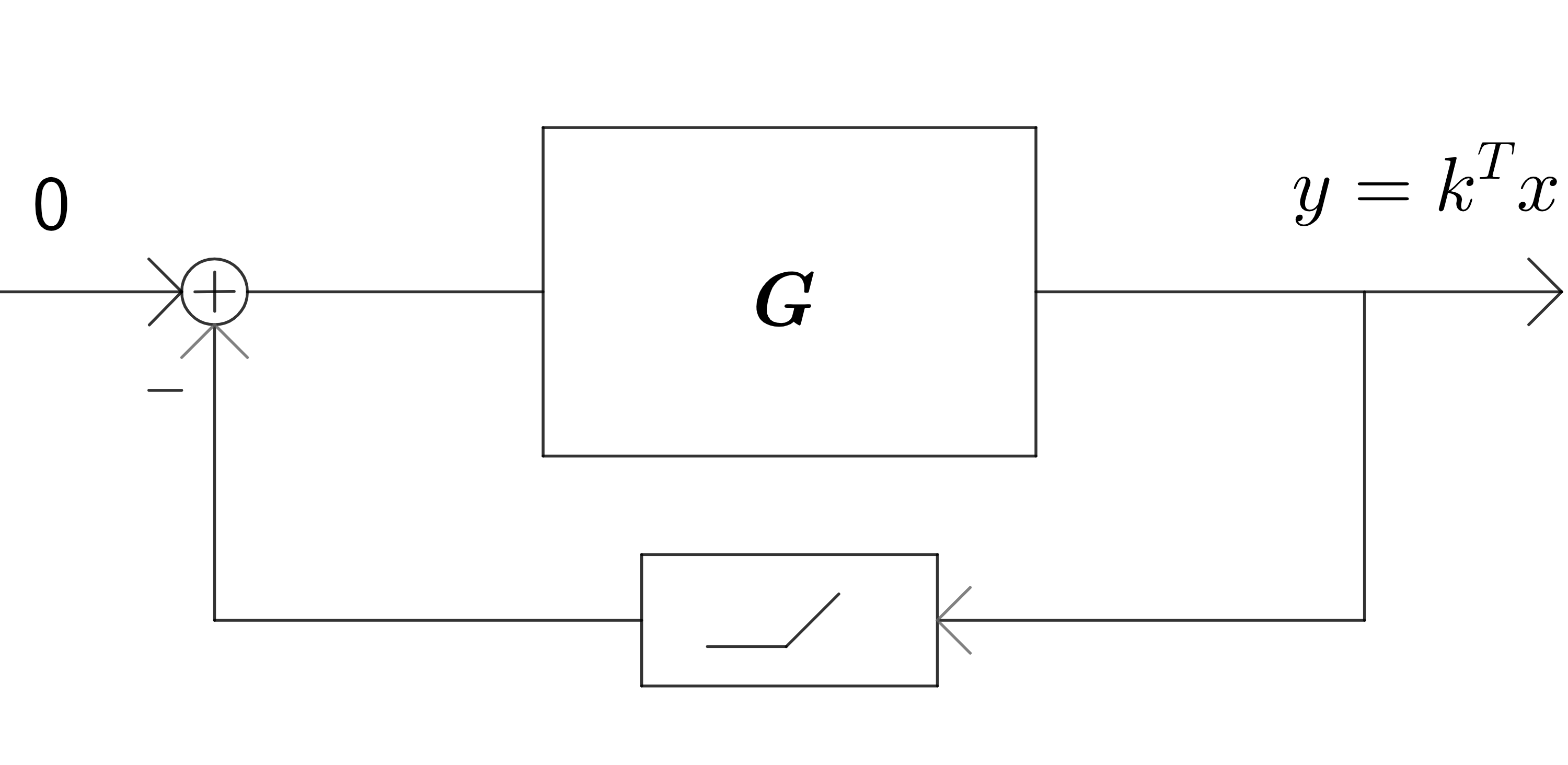
(a) Selector control electrical grid illustrations in the feedback control form

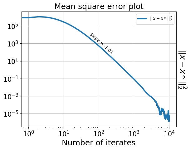
(b) Mean square error plot of the selector control model when $\xi=1$

Figure 1: An example of a non-smooth exponentially stable system with the elector control example.

Note that the slope value $-1.01$ of the linear regressor of the log plot in Figure 1(b) roughly matches the complexity $O\left(\frac{1}{k}\right)$ for $\xi=1$. This empirical result seems to suggest that our complexity bound is tight.

4.2 Nonlinear smooth sub-exponentially stable systems

Now, we consider the following example of a nonlinear system in [23] which represents an example of a smooth sub-exponentially stable system presented in subsection 2.4. Let the dynamic of the nonlinear system be:

$$\begin{cases}\dot{x}_{1}&=-x_{2}-x_{1}^{3}\\ \dot{x}_{2}&=x_{1}-x_{2}^{3}\end{cases}.$$

Under the bounded iterate assumption, this system also satisfies the Lipschitz Assumption 2. Choose the Lyapunov function $V(x_{1},x_{2})=\frac{x_{1}^{2}+x_{2}^{2}}{2}$, we have $V$ is gradient Lipschitz and the time derivative of the Lyapunov function becomes:

$$\dot{V} =x_{1}\dot{x}_{1}+x_{2}\dot{x}_{2}=x_{1}(-x_{2}-x_{1}^{3})+x_{2}(x_{1}-x_{2}^{3})$$

$$=-(x_{1}^{4}+x_{2}^{4})\leq-\frac{(x_{1}^{2}+x_{2}^{2})^{2}}{2}=-2V^{2}$$

Thus, the system satisfies Assumption 5 and Assumption 9 for $c=2$ and $\gamma=2$. Given that these Assumptions are satisfied, we can apply Theorem 2.3 and expect that the system will converge at the rate of $O\left(\frac{1}{k^{\frac{\xi}{c}}}\right)$. We obtain the following plots:

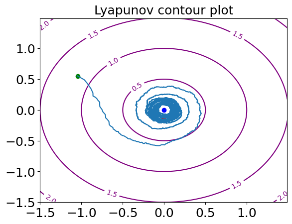
(a) Trajectory of the system

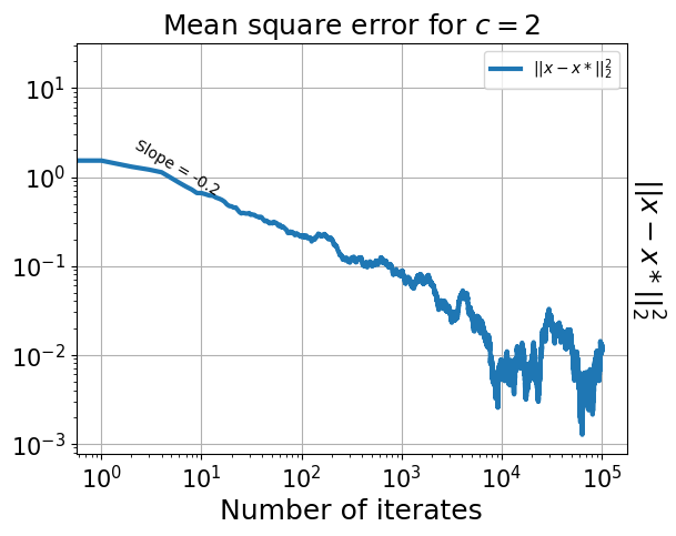
(b) Mean square error plot of the problem when $\xi=0.4$.

Figure 2: Smooth nonlinear system example from [23]

Note that the slope value of the log plot in Figure 2(b) roughly matches the complexity $O\left(\frac{1}{k^{\frac{\xi}{c}}}\right)$ for $\xi=0.4,c=2$, which is $O\left(\frac{1}{k^{0.2}}\right)$. Thus, the empirical performance of our algorithm also validates the theoretical bounds.

4.3 Nonlinear non-smooth sub-exponentially stable systems

In this subsection, we consider the Artstein’s circle example which is a common example for the discontinuous Caratheodory systems. This example is notable since it cannot be stabilized by any continuous feedback [51]. The dynamics can be described as follows:

$$\begin{cases}\dot{x}&=(x^{2}-y^{2})u\\ \dot{y}&=2xyu\end{cases}$$

where $u(x,y)$ is the discontinuous feedback control such that $u(x,y)=-1$ if $x\geq 0$ and $u(x,y)=1$ otherwise [51]. While the system is nonlinear, we can choose $D$ sufficiently large such that the norm ball radius $D$ contains $x^{*}$ and project the iterates onto this norm ball to ensure that they are properly contained inside the norm ball. When the iterates are bounded, the Assumption 2 is satisfied. Choose the Lyapunov function $V(x,y)=\sqrt{4x^{2}+3y^{2}}-|x|$, one can verify that $\dot{V}\leq-\frac{V^{2}}{15}$ and thus $V$ satisfies Assumption 7 for $a=1$ and Assumption 11 for $c=2$ and $\gamma=\frac{1}{15}$, implying sub-exponential stability. This gives $d_{1,2}=1.5$ and we obtain the following empirical results:

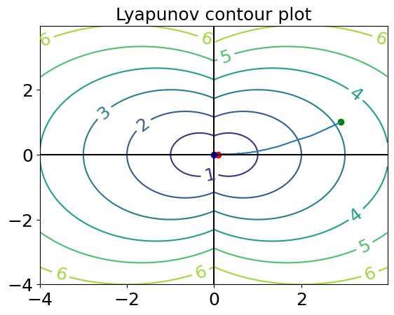
(a) Trajectory of the system

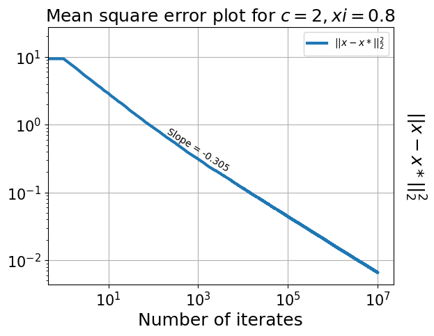
(b) Lyapunov of selector control model when $\xi=0.8$.

Figure 3: Non-smooth Caratheodory system with Artstein’s circle example

While the plots suggest that the algorithm was able to converge, note that the slope value $-0.305$ of the linear regressor of the log plot in Figure 3(b) does not match the complexity $O\left(\frac{1}{k^{\frac{\xi}{2d_{a,c}}}}\right)$ for $\xi=0.8,a=1,c=2$, which is $O\left(k^{-\frac{4}{15}}\right)$. Given the gap between the theoretical guarantee and the empirical performance, we conjecture that the convergence rate of $O\left(\frac{1}{k^{\frac{\xi}{2d_{a,c}}}}\right)$ for $\xi\in\left(0,\frac{2d_{a,c}}{3d_{a,c}-1}\right)$ and $O\left(\frac{1}{k^{\frac{1}{3d_{a,c}-1}}}\right)$ for $\xi=\frac{2d_{a,c}}{3d_{a,c}-1}$ is yet to be optimal.

5 Conclusion and Future works

In this work, we have obtained the finite-time bounds of the stochastic approximation algorithm for a class of problems. While the obtained rates are tight, we suspect that these are yet to be optimal. For example, in the non-smooth case the complexity $O\left(\frac{1}{\varepsilon}\right)$ of the exponentially stable case and the complexity $O\left(\frac{1}{\varepsilon^{3d_{a,c}-1}}\right)$ of the sub-exponentially stable case do not match for $c=1$ due to the use of a time-varying smoothness parameter. Thus, the problem of obtaining optimal rates is still open for future work.

6 Acknowledgements

This work was partially supported by NSF grants EPCN-2144316 and CPS-2240982. The author H.H.N. also kindly thanks Sajad Khodadadian, Sushil Varma, and the anonymous referees for their suggestions to make the paper more clear and readable.

7 Appendix

7.1 Proof of useful lemmas

Recall that in the proof outline for the non-smooth systems, we need to show that the existing properties of the Lyapunov function $V$ such as 7, 11 and 8 are all preserved after we take the infimal convolution of $V$. Thus, in this subsection, we will provide the proofs of some supplementary lemmas of the rescaled Lyapunov function $R$ and the properties of the Moreau envelope. For any polynomially bounded Lyapunov function $V$, a rescale step to make the function quadratically bounded is necessary in order to ensure the resulting Moreau envelope is smooth and also quadratically bounded. Therefore, we will show that the assumptions 7, 11 and 8 still more or less hold for $R=V^{\frac{2}{a}}$.

Lemma 7.1.

Let $R=V^{\frac{2}{a}}$ and $M=R\square\frac{1}{\mu}\left\lVert x\right\rVert_{2}^{2}$, we have that:

• $C_{1}^{\frac{2}{a}}\left\lVert x-x^{*}\right\rVert^{2}\leq R(x)\leq C_{2}^{\frac{2}{a}}\left\lVert x-x^{*}\right\rVert^{2}$

• $M$ is convex and $\frac{1}{\mu}$-smooth

• $\exists 0\leq a<b:(1+a)M(x)\leq R(x)\leq(1+b)M(x)$

• If $R$ is a norm then $M$ is also a norm

Proof.

The first and third property follow from lemma 2.1 in [7].

For the second property, we have:

$$M(x)=\min_{u\in\mathbb{R}^{d}}\left\{R(u)+\frac{\left\lVert x-u\right\rVert_{s}^{2}}{2\mu}\right\}\leq R(x)$$ (18)

which equality holds when $u=x$. For the LHS, note that from the Assumption 7:

$$C_{1}\left\lVert x-x^{*}\right\rVert^{a}\leq V(x)\leq C_{2}\left\lVert x-x^{*}\right\rVert^{a}$$

$$C_{1}^{\frac{2}{a}}\left\lVert x-x^{*}\right\rVert^{2}\leq R(x)=V(x)^{\frac{2}{a}}\leq C_{2}^{\frac{2}{a}}\left\lVert x-x^{*}\right\rVert^{2}$$

Thus, we have:

$$M(x) =\min_{u\in\mathbb{R}^{d}}\left\{R(u)+\frac{\left\lVert x-u\right\rVert_{s}^{2}}{2\mu}\right\}$$

$$\geq\min_{u\in\mathbb{R}^{d}}\left\{C_{1}^{\frac{2}{a}}\left\lVert u-x^{*}\right\rVert_{s}^{2}+\frac{(\left\lVert x-x^{*}\right\rVert_{s}-\left\lVert u-x^{*}\right\rVert_{s})^{2}}{2\mu}\right\}$$

$$\geq\frac{\left\lVert x-x^{*}\right\rVert_{s}^{2}}{\frac{1}{C_{1}^{\frac{2}{a}}}+2\mu}\geq\frac{R(x)}{\frac{C_{2}^{\frac{2}{a}}}{C_{1}^{\frac{2}{a}}}+2C_{2}^{\frac{2}{a}}\mu}$$

$$\Leftrightarrow R(x) \leq\left(\frac{C_{2}^{\frac{2}{a}}}{C_{1}^{\frac{2}{a}}}+2C_{2}^{\frac{2}{a}}\mu\right)M(x)$$ (19)

∎

Lemma 7.1 allows us to quantify how well $M$ approximates $R$ and its smoothness in terms of $\mu$. While smaller $\mu$ gives a better approximation of $R$, it also scales inversely with the smoothness parameter.

Lemma 7.2.

Let $R=V^{\frac{2}{a}}$ and $M=V\square\frac{1}{2\mu}\left\lVert x\right\rVert_{2}^{a}$, we have $\nabla M(x)=\frac{x-u}{\mu}$ and for $G_{M}=\frac{2}{a}GC_{2}^{\frac{2}{a}-1}$:

$$\left\lVert\nabla M(x)\right\rVert=\left\lVert\frac{x-u}{\mu}\right\rVert\leq G_{M}\left\lVert u-x^{*}\right\rVert$$ (20)

Proof.

From the Envelope Theorem [14], we have that $\nabla M(x)=\frac{x-u}{\mu}$. From 14, we have $\nabla M(x)\in\partial R(u)$ due to the Fundamental Theorem of Calculus. Furthermore, notice that from Assumptions 7 and 8, we obtain that:

$$\left\lVert\frac{\partial V}{\partial x}\right\rVert \leq G\left\lVert x-x^{*}\right\rVert^{a-1}$$

$$\Rightarrow\left\lVert\frac{\partial R}{\partial x}\right\rVert=\frac{2}{a}V^{\frac{2}{a}-1}\left\lVert\frac{\partial V}{\partial x}\right\rVert \leq\frac{2}{a}GC_{2}^{\frac{2}{a}-1}\left\lVert x-x^{*}\right\rVert\forall x\in\mathbb{R}^{d}$$

and since $\nabla M(x)\in\partial R(prox(x))$ and $u=prox(x)$, we have:

$$\left\lVert\nabla M(x)\right\rVert=\left\lVert\frac{x-u}{\mu}\right\rVert\leq\frac{2}{a}GC_{2}^{\frac{2}{a}-1}\left\lVert u-x^{*}\right\rVert=G_{M}\left\lVert u-x^{*}\right\rVert\forall x\in\mathbb{R}^{d}$$

∎

Conveniently, Lemma 7.2 allows us to obtain a lower bound of $\left\lVert u-x^{*}\right\rVert$ in terms of $\left\lVert x-x^{*}\right\rVert$ and $\mu$. This comes from the intuition that $prox(x)$ and $x$ cannot be too far from each other and as $\mu\rightarrow 0$, $prox(x)$ should approach $x$.

Corollary 7.2.1.

Let $u=prox(x)$ and $G_{M}=\frac{2}{a}GC_{2}^{\frac{2}{a}-1}$, we have:

$$\left\lVert u-x^{*}\right\rVert_{2} \geq\frac{\left\lVert x-x^{*}\right\rVert_{2}}{1+\mu G_{M}}\forall x\in\mathbb{R}^{d},\mu>0$$

Proof.

From 7.2, we have $\left\lVert\nabla M(x)\right\rVert=\left\lVert\frac{x-u}{\mu}\right\rVert\leq G_{M}\left\lVert u-x^{*}\right\rVert\forall x\in\mathbb{R}^{d}$, thus by triangle inequality:

$$\frac{\left\lVert x-x^{*}\right\rVert-\left\lVert u-x^{*}\right\rVert}{\mu}\leq\left\lVert\frac{x-u}{\mu}\right\rVert\leq G_{M}\left\lVert u-x^{*}\right\rVert$$

$$\Rightarrow\frac{\left\lVert x-x^{*}\right\rVert_{2}}{1+\mu G_{M}}\leq\left\lVert u-x^{*}\right\rVert_{2}$$

∎

Lemma 7.3.

(Negative drift of $R$) Assume that $V$ satisfies Assumptions 7, 11 and let $R=V^{\frac{2}{a}}$, we have that:

$$\langle\nabla R(x),F(x)\rangle\leq-\frac{2\gamma_{c}}{a}R(x)^{\frac{a(c-1)}{2}+1}$$ (21)

Proof.

By applying chain rule, we have:

$$\langle\nabla R(x),F(x)\rangle =\frac{2}{a}V^{\frac{2}{a}-1}\langle\nabla V(x),F(x)\rangle$$

$$\leq-\frac{2}{a}V^{\frac{2}{a}-1}\gamma_{c}V(x)^{c}\text{ from Assumption \ref{assumption: clarke-asymptotic-stability}}$$

$$=-\frac{2\gamma_{c}}{a}R(x)^{\frac{a(c-1)}{2}+1}$$

Hence proved. ∎

Lemma 7.3 shows that if $V$ has a negative drift then $R=V^{\frac{2}{a}}$ also has a negative drift. Lemma 7.2 and Lemma 7.3 allow us to reduce the problem to when $a=2$ where $a$ is the constant in Assumption 7.

Lemma 7.4.

(Change of smoothness parameter bound) For $0<\mu<\mu^{\prime}$ and $G_{M}=\frac{2}{a}GC_{2}^{\frac{2}{a}-1}$, we have:

$$M_{\mu}(x)-M_{\mu^{\prime}}(x)\leq(\mu^{\prime}-\mu)G_{M}^{2}\left\lVert x-x^{*}\right\rVert^{2}\forall x\in\mathbb{R}^{d}$$ (22)

Proof.

From the Gradient Theorem for line integrals, we have $\forall x\in\mathbb{R}^{d}$:

$$M_{\mu}(x)-M_{\mu^{\prime}}(x) =\int_{\mu^{\prime}}^{\mu}\frac{\partial M(x)}{\partial\mu}d\tau$$

$$=\int_{\mu^{\prime}}^{\mu}-\left\lVert\nabla M_{\tau}(x)\right\rVert^{2}d\tau=\int_{\mu}^{\mu^{\prime}}\left\lVert\nabla M_{\tau}(x)\right\rVert^{2}d\tau$$

$$\leq\int_{\mu}^{\mu^{\prime}}\left(\frac{2GC_{2}^{\frac{2}{a}-1}}{a}\right)^{2}\left\lVert x-x^{*}\right\rVert^{2}d\tau=(\mu^{\prime}-\mu)\left(\frac{2GC_{2}^{\frac{2}{a}-1}}{a}\right)^{2}\left\lVert x-x^{*}\right\rVert^{2}$$

where $\frac{\partial M(x)}{\partial\mu}=-\left\lVert\nabla M_{\mu}(x)\right\rVert^{2}$ [52] and the last inequality follows from 7.2. Hence proved. ∎

7.2 Proof of the main results

Here, we will provide detailed proofs of the settings we included in the main results. We will first present the proofs for the non-smooth exponentially stable setting and then proceed to the smooth exponentially stable setting since the proof of the latter largely follows the arguments in the former setting once we have constructed a smooth Lyapunov function using the Moreau envelope. Later on, we will provide proof for the smooth sub-exponentially stable setting in the subsection 7.2.3 and the non-smooth sub-exponentially stable setting in the subsection 7.2.4.

7.2.1 Nonsmooth exponentially stable case

In this subsection, we will give a detailed proof of the finite-time convergence of non-smooth exponentially stable systems. Consider $R=V^{\frac{2}{a}}$ and let $M=R\square\frac{\left\lVert x\right\rVert^{2}}{2\mu},G_{M}=\frac{2}{a}GC_{2}^{\frac{2}{a}-1}$, we will show that $M$ will also have a negative drift:

Lemma 7.5.

There exists a constant $0<\gamma_{M}<\frac{2\gamma}{a}\left(\frac{C_{1}}{C_{2}}\right)^{\frac{2}{a}}$ such that for sufficiently small $\mu>0$:

$$\langle\nabla M(x),F(x)\rangle\leq-\gamma_{M}M(x)\forall x\in\mathbb{R}^{d}$$

Proof.

Recall that $u=prox(x)$. Since $\nabla M(x)=\frac{x-u}{\mu}=g_{u}\in\partial R(u)$, we have:

$$\langle\nabla M(x),F(x)\rangle =\langle g_{u},F(u)\rangle+\langle g_{u},F(x)-F(u)\rangle$$

$$\leq-\frac{2\gamma}{a}R(u)+C\left\lVert x-u\right\rVert\left\lVert\nabla M(x)\right\rVert$$

$$\leq-\frac{2\gamma C_{1}^{\frac{2}{a}}}{a\left(1+\mu G_{M}\right)^{2}}\left\lVert x-x^{*}\right\rVert^{2}+\mu CG_{M}^{2}\left\lVert u-x^{*}\right\rVert^{2}$$

$$\leq\left[-\frac{2\gamma C_{1}^{\frac{2}{a}}}{a\left(1+\mu G_{M}\right)^{2}}+\mu CG_{M}^{2}\right]\left\lVert x-x^{*}\right\rVert^{2}$$

where the first inequality is from Lemma 7.3, Cauchy-Schwarz inequality and Assumption 2, the second one is from Assumption 7, Lemma 7.2 and Corollary 7.2.1 and the last one follows from the non-expansiveness of the proximal operator. Since $0<\gamma_{M}<\frac{2\gamma}{a}\left(\frac{C_{1}}{C_{2}}\right)^{\frac{2}{a}}$, we can choose $\mu$ small enough such that $-\frac{2\gamma C_{1}^{\frac{2}{a}}}{a\left(1+\mu G_{M}\right)^{2}}+\mu CG_{M}^{2}\leq-\gamma_{M}C_{2}^{\frac{2}{a}}$. From here, we are done since:

$$\left[-\frac{2\gamma C_{1}^{\frac{2}{a}}}{a\left(1+\mu G_{M}\right)^{2}}+\mu CG_{M}^{2}\right]\left\lVert x-x^{*}\right\rVert^{2}\leq-\gamma_{M}C_{2}^{\frac{2}{a}}\left\lVert x-x^{*}\right\rVert^{2}\leq-\gamma_{M}R(x)$$

and by the definition of Moreau envelope, note that $M(x)\leq R(x)\forall x\in\mathbb{R}^{d}$. Thus $\forall x\in\mathbb{R}^{d}$, we have:

$$\langle\nabla M(x),F(x)\rangle\leq\left[-\frac{2\gamma C_{1}^{\frac{2}{a}}}{a\left(1+\mu G_{M}\right)^{2}}+\mu CG_{M}^{2}\right]\left\lVert x-x^{*}\right\rVert^{2}\leq-\gamma_{M}M(x)$$

Hence proved. ∎

Now, the existence of the negative drift would allow us to obtain a contraction on $M$ with some noise via some first-order bounds (such as the smoothness inequality). From here and given that $\mu$ is chosen to be sufficiently small, we first obtain the one-iterate bound as follows:

Theorem 7.6.

Assume that we have chosen a sufficiently small $\mu$ such that $\exists\gamma_{M}\in\left(0,\frac{2\gamma}{a}\left(\frac{C_{1}}{C_{2}}\right)^{\frac{2}{a}}\right)$ such that $\gamma_{M}=-\left[-\frac{2\gamma C_{1}^{\frac{2}{a}}}{a\left(1+\mu G_{M}\right)^{2}}+\mu CG_{M}^{2}\right]C_{2}^{-\frac{2}{a}}$. We have:

$$\mathbb{E}[M(x_{k})|\mathcal{F}_{k}]\leq\left(1-\alpha_{k-1}\gamma_{M}+\frac{\alpha_{k-1}^{2}(C^{2}+2B)}{2\mu^{2}+\frac{\mu}{C_{1}}}\right)M(x_{k-1})+\frac{\alpha_{k-1}^{2}(A+2B\left\lVert x^{*}\right\rVert_{2}^{2})}{\mu}$$

Proof.

Consider $R=V^{\frac{2}{a}}$, we have:

$$C_{1}^{\frac{2}{a}}\left\lVert x-x^{*}\right\rVert^{2}\leq R(x)\leq C_{2}^{\frac{2}{a}}\left\lVert x-x^{*}\right\rVert^{2}\forall x\in\mathbb{R}^{d}$$

and

$$\dot{R} =\langle r_{x},F(x)\rangle\forall r_{x}\in\partial R(x)$$

where $\partial R(x)=\overline{co}\{\lim\nabla R(x)|x_{i}\rightarrow x,x_{i}\not\in\Omega_{V}\}$ is the generalized gradient of $R$. Note that:

$$\nabla R(x)=\frac{2}{a}\nabla V(x)V(x)^{\frac{2}{a}-1}\forall x\not\in\Omega_{V}$$

Hence:

$$\langle r_{x},F(x)\rangle =\frac{2V(x)^{\frac{2}{a}-1}}{a}\langle g_{x},F(x)\rangle\forall r_{x}\in\partial R(x),g_{x}\in\partial V(x)$$

$$\leq\frac{2V(x)^{\frac{2}{a}-1}}{a}\times(-\gamma V(x))$$

$$=-\frac{2\gamma}{a}V(x)^{\frac{2}{a}}=-\frac{2\gamma}{a}R(x)\forall x=-\gamma_{R}R(x)\in\mathbb{R}^{d}$$

where $\gamma_{R}=\frac{2\gamma}{a}$ and the first inequality follows from 3. Furthermore:

$$\left\lVert\frac{\partial V}{\partial x}\right\rVert \leq G\left\lVert x-x^{*}\right\rVert^{a-1}$$

$$\Rightarrow\frac{2}{a}\left\lVert V^{\frac{2}{a}-1}\right\rVert\left\lVert\frac{\partial V}{\partial x}\right\rVert \leq\frac{2}{a}\times C_{2}^{\frac{2}{a}-1}\left\lVert x-x^{*}\right\rVert^{a\times\frac{2-a}{a}}G_{2}\left\lVert x-x^{*}\right\rVert^{a-1}$$

$$\Rightarrow\left\lVert\frac{\partial R}{\partial x}\right\rVert \leq\frac{2GC_{2}^{\frac{2}{a}-1}}{a}\left\lVert x-x^{*}\right\rVert=G_{M}\left\lVert x-x^{*}\right\rVert$$

Thus, we have $R$ satisfies 6, 7 and 8 for $a=2$. Let $M=R\square\frac{\left\lVert x\right\rVert^{2}}{2\mu}$, from the $\frac{1}{\mu}$-smoothness of $M$, we obtain:

$$M(x_{k}) \leq M(x_{k-1})+\langle\nabla M(x_{k-1}),x_{k}-x_{k-1}\rangle+\frac{1}{2\mu}\left\lVert x_{k}-x_{k-1}\right\rVert_{2}^{2}$$

Taking expectations on both sides, we have:

$$E_{k}=\mathbb{E}[M(x_{k})|\mathcal{F}_{k-1}]\leq M(x_{k-1})+\alpha_{k-1}\langle\nabla M(x_{k-1}),F(x_{k-1})\rangle+\frac{\alpha_{k-1}^{2}\mathbb{E}[\left\lVert F(x_{k-1})+w_{k-1}\right\rVert^{2}|\mathcal{F}_{k-1}]}{2\mu}$$

Thus, from Lemma 7.5, we have that:

$$\langle\nabla M(x),F(x)\rangle\leq-\gamma_{M}M(x)\forall x\in\mathbb{R}^{d}$$

with $\gamma_{M}=\left[\frac{2\gamma C_{1}^{\frac{2}{a}}}{a\left(1+\mu G_{M}\right)^{2}}-\mu CG_{M}^{2}\right]C_{2}^{-\frac{2}{a}}$. Denote $E_{k}=\mathbb{E}[M(x_{k})|\mathcal{F}_{k-1}]$, we have:

$$E_{k} \leq M(x_{k-1})+\alpha_{k-1}\langle\nabla M(x_{k-1}),F(x_{k-1})\rangle+\frac{\alpha_{k-1}^{2}\mathbb{E}[\left\lVert F(x_{k-1})+w_{k-1}\right\rVert^{2}|\mathcal{F}_{k-1}]}{2\mu}$$

which gives:

$$E_{k} \leq(1-\alpha_{k-1}\gamma_{M})M(x_{k-1})+\frac{\alpha_{k-1}^{2}}{2\mu}\mathbb{E}[\left\lVert F(x_{k-1})+w_{k-1}\right\rVert_{2}^{2}|\mathcal{F}_{k-1}]$$

$$=(1-\alpha_{k-1}\gamma_{M})M(x_{k-1})+\frac{\alpha_{k-1}^{2}}{2\mu}\mathbb{E}[\left\lVert F(x_{k-1})-F(x^{*})+w_{k-1}\right\rVert_{2}^{2}|\mathcal{F}_{k-1}].$$

The RHS can be further bounded as:

$$\overset{(a)}{\leq}(1-\alpha_{k-1}\gamma_{M})M(x_{k-1})+\frac{\alpha_{k-1}^{2}}{2\mu}\mathbb{E}[(\left\lVert F(x_{k-1})-F(x^{*})\right\rVert_{2}+\left\lVert w_{k-1}\right\rVert_{2})^{2}|\mathcal{F}_{k-1}]$$

$$\overset{(b)}{\leq}(1-\alpha_{k-1}\gamma_{M})M(x_{k-1})+\frac{\alpha_{k-1}^{2}}{2\mu}\mathbb{E}[(C\left\lVert x_{k-1}-x^{*}\right\rVert_{2}+\left\lVert w_{k-1}\right\rVert_{2})^{2}|\mathcal{F}_{k-1}]$$

$$\overset{(c)}{\leq}(1-\alpha_{k-1}\gamma_{M})M(x_{k-1})+\frac{\alpha_{k-1}^{2}(C^{2}\left\lVert x_{k-1}-x^{*}\right\rVert_{2}^{2}+\mathbb{E}[\left\lVert w_{k-1}\right\rVert_{2}^{2}|\mathcal{F}_{k-1}])}{\mu}$$

$$\overset{(d)}{\leq}(1-\alpha_{k-1}\gamma_{M})M(x_{k-1})+\frac{\alpha_{k}^{2}(C^{2}\left\lVert x_{k-1}-x^{*}\right\rVert_{2}^{2}+A+B\left\lVert x_{k-1}\right\rVert_{2}^{2})}{\mu}$$

$$\overset{(e)}{\leq}(1-\alpha_{k-1}\gamma_{M})M(x_{k-1})+\frac{\alpha_{k}^{2}(C^{2}\left\lVert x_{k-1}-x^{*}\right\rVert_{2}^{2}+A+2B\left\lVert x_{k-1}-x^{*}\right\rVert_{2}^{2}+2B\left\lVert x^{*}\right\rVert_{2}^{2})}{\mu}$$

$$=(1-\alpha_{k-1}\gamma_{M})M(x_{k-1})+\frac{\alpha_{k-1}^{2}(C^{2}+2B)\left\lVert x_{k-1}-x^{*}\right\rVert_{2}^{2}}{\mu}+\frac{\alpha_{k-1}^{2}(A+2B\left\lVert x^{*}\right\rVert_{2}^{2})}{\mu}$$

$$\overset{(f)}{\leq}(1-\alpha_{k-1}\gamma_{M})M(x_{k-1})+\frac{\alpha_{k-1}^{2}(C^{2}+2B)M(x_{k-1})}{\mu\left(\frac{1}{C_{1}^{\frac{2}{a}}}+2\mu\right)}+\frac{\alpha_{k-1}^{2}(A+2B\left\lVert x^{*}\right\rVert_{2}^{2})}{\mu}$$

$$=\left(1-\alpha_{k-1}\gamma_{M}+\frac{\alpha_{k-1}^{2}(C^{2}+2B)}{2\mu^{2}+\frac{\mu}{C_{1}^{\frac{2}{a}}}}\right)M(x_{k-1})+\frac{\alpha_{k-1}^{2}(A+2B\left\lVert x^{*}\right\rVert_{2}^{2})}{\mu}`$$

The first inequality (a) follows from triangle inequality, the second inequality (b) follows from Assumption 2, the third inequality (c) follows from Cauchy-Schwarz, the fourth inequality (d) follows from the Assumption 1 and the last inequality (f) follows from 7.1. Hence, we are done. ∎

From the one-iterate bound 7.6, we can expand all the terms by applying the result repeatedly. Then, with appropriate choice of step size of the form $\alpha_{k}=\frac{\alpha}{(k+K)^{\xi}}$ where $\alpha>0,\xi\in[0,1]$ where $K$ is chosen such that $\alpha_{k}\leq\frac{\gamma_{M}\left(2\mu^{2}+\frac{\mu}{C_{1}^{\frac{2}{a}}}\right)}{2(C^{2}+2B)}\forall k\in\mathbb{Z}^{+}$.

Proposition 1.

Suppose that $V$ satisfies assumptions 7, 6 and 8 and let

$$\gamma_{M}=-\left[-\frac{2\gamma C_{1}^{\frac{2}{a}}}{a\left(1+\mu G_{M}\right)^{2}}+\mu CG_{M}^{2}\right]C_{2}^{-\frac{2}{a}},\alpha_{0}\leq\frac{2(C^{2}+2B)}{\gamma_{M}\left(2\mu^{2}+\frac{\mu}{C_{1}^{\frac{2}{a}}}\right)}$$

then we have:

$$\mathbb{E}[M(x_{k})|\mathcal{F}_{k}]\leq C_{2}^{\frac{2}{a}}\left\lVert x_{0}-x^{*}\right\rVert_{2}^{2}\prod_{j=0}^{k-1}\left(1-\frac{\alpha_{j}\gamma_{M}}{2}\right)+\left[\sum_{i=0}^{k-1}\alpha_{i}^{2}\prod_{j=i+1}^{k-1}\left(1-\frac{\alpha_{j}\gamma_{M}}{2}\right)\right]\frac{A+2B\left\lVert x^{*}\right\rVert_{2}^{2}}{\mu}$$

Proof.

By our choice of $\alpha_{k}$ and from the lemma 7.6, we have:

$$\mathbb{E}[M(x_{k})|\mathcal{F}_{k-1}] \leq\left(1-\frac{\alpha_{k-1}\gamma_{M}}{2}\right)M(x_{k-1})+\frac{\alpha_{k-1}^{2}(A+2B\left\lVert x^{*}\right\rVert_{2}^{2})}{\mu}$$

$$\Rightarrow\mathbb{E}[M(x_{k})|\mathcal{F}_{k-1}] \leq\prod_{j=0}^{k-1}\left(1-\frac{\alpha_{j}\gamma_{M}}{2}\right)M(x_{0})+\left[\sum_{i=0}^{k-1}\alpha_{i}^{2}\prod_{j=i+1}^{k-1}\left(1-\frac{\alpha_{j}\gamma_{M}}{2}\right)\right]\frac{A+2B\left\lVert x^{*}\right\rVert_{2}^{2}}{\mu}$$

$$\leq C_{2}^{\frac{2}{a}}\left\lVert x_{0}-x^{*}\right\rVert_{2}^{2}\prod_{j=0}^{k-1}\left(1-\frac{\alpha_{j}\gamma_{M}}{2}\right)+\left[\sum_{i=0}^{k-1}\alpha_{i}^{2}\prod_{j=i+1}^{k-1}\left(1-\frac{\alpha_{j}\gamma_{M}}{2}\right)\right]\frac{A+2B\left\lVert x^{*}\right\rVert_{2}^{2}}{\mu}$$

∎

From this one-iterate bound, we expand all the terms and obtain the finite-time bounds depending on the chosen step sizes. The detailed description and proof of the finite-time bounds are presented below:

Theorem 7.7.

Under the Assumptions 1, 2 and suppose that there exists a Lyapunov function V satisfying the assumptions 5, 6 and 8, the rate of convergence for the stochastic approximation problem is:
For $\xi=1$:

$$\mathbb{E}[\left\lVert x_{k}-x^{*}\right\rVert_{2}^{2}] \leq C_{2}^{\frac{2}{a}}\left(\frac{1}{C_{1}^{\frac{2}{a}}}+2\mu\right)\left\lVert x_{0}-x^{*}\right\rVert_{2}^{2}\left(\frac{K}{k+K}\right)^{\frac{\alpha\gamma_{M}}{2}}$$

$$+\left(\frac{1}{C_{1}^{\frac{2}{a}}}+2\mu\right)\times\begin{cases}\frac{8\alpha^{2}}{2-\alpha\gamma_{M}}\frac{1}{(k+K)^{\frac{\alpha\gamma_{M}}{2}}}\frac{A+2B\left\lVert x^{*}\right\rVert_{2}^{2}}{\mu}&\text{ if }\alpha\in\left(0,\frac{2}{\gamma_{M}}\right)\\ \frac{4\alpha^{2}\log(k+K)}{k+K}\frac{A+2B\left\lVert x^{*}\right\rVert_{2}^{2}}{\mu}&\text{ if }\alpha=\frac{2}{\gamma_{M}}\\ \frac{8e\alpha^{2}}{\alpha\gamma_{M}-2}\frac{1}{k+K}\frac{A+2B\left\lVert x^{*}\right\rVert_{2}^{2}}{\mu}&\text{ if }\alpha\in\left(\frac{2}{\gamma_{M}},\infty\right)\end{cases}$$

For $\xi\in(0,1)$:

$$\mathbb{E}[\left\lVert x_{k}-x^{*}\right\rVert_{2}^{2}] \leq C_{2}^{\frac{2}{a}}\left(\frac{1}{C_{1}^{\frac{2}{a}}}+2\mu\right)\left\lVert x_{0}-x^{*}\right\rVert_{2}^{2}\exp\left[-\frac{\alpha\gamma_{M}}{2(1-\xi)}((k+K)^{1-\xi}-K^{1-\xi})\right]$$

$$+\frac{4\alpha\left(\frac{1}{C_{1}^{\frac{2}{a}}}+2\mu\right)}{\gamma_{M}(k+K)^{\xi}}\frac{A+2B\left\lVert x^{*}\right\rVert_{2}^{2}}{\mu}$$

For $\xi=0$:

$$\mathbb{E}[\left\lVert x_{k}-x^{*}\right\rVert_{2}^{2}]\leq C_{2}^{\frac{2}{a}}\left(\frac{1}{C_{1}^{\frac{2}{a}}}+2\mu\right)\left\lVert x_{0}-x^{*}\right\rVert_{2}^{2}\left(1-\frac{\alpha\gamma_{M}}{2}\right)^{k}+\left(\frac{1}{C_{1}^{\frac{2}{a}}}+2\mu\right)\frac{2(A+2B\left\lVert x^{*}\right\rVert_{2}^{2})\alpha}{\mu\gamma_{M}}$$

where $K=\max\left\{1,\frac{\alpha(4C^{2}+8B)}{\gamma}\right\}$ for $\xi=1$ and $K=\max\left\{1,\left(\frac{\alpha(4C^{2}+8B)}{\gamma}\right)^{\frac{1}{\xi}},\left(\frac{2\xi}{\alpha\gamma}\right)^{\frac{1}{1-\xi}}\right\}$ for $\xi\in(0,1)$.

Proof.

From Proposition (1), we have:

$$\mathbb{E}[M(x_{k})|\mathcal{F}_{k-1}]\leq C_{2}^{\frac{2}{a}}\left\lVert x_{0}-x^{*}\right\rVert_{2}^{2}\prod_{j=0}^{k-1}\left(1-\frac{\alpha_{j}\gamma_{M}}{2}\right)+\left[\sum_{i=0}^{k-1}\alpha_{i}^{2}\prod_{j=i+1}^{k-1}\left(1-\frac{\alpha_{j}\gamma_{M}}{2}\right)\right]\frac{A+2B\left\lVert x^{*}\right\rVert_{2}^{2}}{\mu}.$$

Note that $M(x)\geq\frac{\left\lVert x-x^{*}\right\rVert^{2}}{C_{1}^{-\frac{2}{a}}+2\mu}\forall x\in\mathbb{R}^{d}$. Hence:

$$\mathbb{E}[\left\lVert x_{k}-x^{*}\right\rVert^{2}] \leq C_{2}^{\frac{2}{a}}\left(\frac{1}{C_{1}^{\frac{2}{a}}}+2\mu\right)\left\lVert x_{0}-x^{*}\right\rVert_{2}^{2}\prod_{j=1}^{k-1}\left(1-\frac{\alpha_{j}\gamma_{M}}{2}\right)$$

$$+\left[\sum_{i=0}^{k-1}\alpha_{i}^{2}\prod_{j=i+1}^{k-1}\left(1-\frac{\alpha_{j}\gamma_{M}}{2}\right)\right]\frac{\left(A+2B\left\lVert x^{*}\right\rVert_{2}^{2}\right)\left(\frac{1}{C_{1}^{\frac{2}{a}}}+2\mu\right)}{\mu}$$ (23)

Note that:

$$C_{2}^{\frac{2}{a}}\left\lVert x_{0}-x^{*}\right\rVert_{2}^{2}\prod_{i=0}^{k-1}\left(1-\frac{\alpha_{i}\gamma_{M}}{2}\right) \leq C_{2}^{\frac{2}{a}}\left\lVert x_{0}-x^{*}\right\rVert_{2}^{2}e^{-\frac{\gamma_{M}}{2}\sum_{i=0}^{k}\alpha_{i}}$$

$$=C_{2}^{\frac{2}{a}}\left\lVert x_{0}-x^{*}\right\rVert_{2}^{2}e^{-\frac{\alpha\gamma_{M}}{2}\sum_{i=0}^{k-1}\frac{1}{(i+K)^{\xi}}}$$ (24)

and since $\int_{a}^{b+1}h(x)dx\leq\sum_{n=a}^{n}h(n)\leq\int_{a-1}^{b}h(x)dx$ for any non-increasing function $h$, we have for $\xi=1$:

$$C_{2}^{\frac{2}{a}}\left\lVert x_{0}-x^{*}\right\rVert_{2}^{2}\prod_{i=0}^{k-1}\left(1-\frac{\alpha_{i}\gamma_{M}}{2}\right)\leq C_{2}^{\frac{2}{a}}\left\lVert x_{0}-x^{*}\right\rVert_{2}^{2}\left(\frac{K}{k+K}\right)^{\frac{\alpha\gamma_{M}}{2}}.$$ (25)

and for $\xi\in(0,1)$:

$$C_{2}^{\frac{2}{a}}\left\lVert x_{0}-x^{*}\right\rVert_{2}^{2}\prod_{i=0}^{k-1}\left(1-\frac{\alpha_{i}\gamma_{M}}{2}\right)\leq C_{2}^{\frac{2}{a}}\left\lVert x_{0}-x^{*}\right\rVert_{2}^{2}\exp\left[-\frac{\alpha\gamma_{M}}{2(1-\xi)}((k+K)^{1-\xi}-K^{1-\xi})\right].$$ (26)

Next, we need to bound the second term. For $\xi=1$, we have:

$$\sum_{i=0}^{k-1}\alpha_{i}^{2}\prod_{j=i+1}^{k-1}\left(1-\frac{\alpha_{j}\gamma_{M}}{2}\right) =\alpha^{2}\sum_{i=0}^{k-1}\frac{1}{(i+K)^{2}}\prod_{j=i+1}^{k-1}\left(1-\frac{\alpha_{j}\gamma_{M}}{2}\right)$$

$$\leq\alpha^{2}\sum_{i=0}^{k-1}\frac{1}{(i+K)^{2}}\exp\left(-\frac{\alpha\gamma_{M}}{2}\sum_{j=i+1}^{k-1}\frac{1}{j+K}\right)$$

$$\leq\alpha^{2}\sum_{i=0}^{k-1}\frac{1}{(i+K)^{2}}\exp\left(-\frac{\alpha\gamma_{M}}{2}\int_{i+1}^{k}\frac{1}{j+K}dj\right)$$

$$\leq\alpha^{2}\sum_{i=0}^{k-1}\frac{1}{(i+K)^{2}}\left(\frac{i+1+K}{k+K}\right)^{\frac{\alpha\gamma_{M}}{2}}$$

$$\leq\frac{4\alpha^{2}}{(k+K)^{\frac{\alpha\gamma_{M}}{2}}}\sum_{i=0}^{k-1}\frac{1}{(i+1+K)^{2-\frac{\alpha\gamma_{M}}{2}}}$$

∎

This proof follows from [7]. Now, it is sufficient to do casework for $\alpha\gamma_{M}$. We have:

• $\alpha\gamma_{M}\in(0,2)\Rightarrow\sum_{i=0}^{k-1}\frac{1}{(i+1+K)^{2-\frac{\alpha\gamma_{M}}{2}}}\leq\frac{2}{2-\alpha\gamma_{M}}$

• $\alpha\gamma_{M}=2\Rightarrow\sum_{i=0}^{k-1}\frac{1}{(i+1+K)^{2-\frac{\alpha\gamma_{M}}{2}}}\leq\log(k+K)$

• $\alpha\gamma_{M}\in(2,4)\Rightarrow\sum_{i=0}^{k-1}\frac{1}{(i+1+K)^{2-\frac{\alpha\gamma_{M}}{2}}}\leq\frac{2(k+K)^{\alpha\gamma_{M}-2}}{\alpha\gamma_{M}-2}$

• $\alpha\gamma_{M}=4\Rightarrow\sum_{i=0}^{k-1}\frac{1}{(i+1+K)^{2-\frac{\alpha\gamma_{M}}{2}}}=k$

• $\alpha\gamma_{M}\in(4,+\infty)\Rightarrow\sum_{i=0}^{k-1}\frac{1}{(i+1+K)^{2-\frac{\alpha\gamma_{M}}{2}}}\leq\frac{e(k+K)^{\frac{\alpha\gamma_{M}-2}{2}}}{\frac{\alpha\gamma_{M}}{2}-1}$

Thus for $\xi=1$, we have:

• $\alpha\gamma_{M}\in(0,2)\Rightarrow\frac{4\alpha^{2}}{(k+K)^{\frac{\alpha\gamma_{M}}{2}}}\sum_{i=0}^{k-1}\frac{1}{(i+1+K)^{2-\frac{\alpha\gamma_{M}}{2}}}\leq\frac{8\alpha^{2}}{2-\alpha\gamma_{M}}\frac{1}{(k+K)^{\frac{\alpha\gamma_{M}}{2}}}$

• $\alpha\gamma_{M}=2\Rightarrow\frac{4\alpha^{2}}{(k+K)^{\frac{\alpha\gamma_{M}}{2}}}\sum_{i=0}^{k-1}\frac{1}{(i+1+K)^{2-\frac{\alpha\gamma_{M}}{2}}}\leq\frac{4\alpha^{2}\log(k+K)}{k+K}$

• $\alpha\gamma_{M}\in(2,+\infty)\Rightarrow\frac{4\alpha^{2}}{(k+K)^{\frac{\alpha\gamma_{M}}{2}}}\sum_{i=0}^{k-1}\frac{1}{(i+1+K)^{2-\frac{\alpha\gamma_{M}}{2}}}\leq\frac{8e\alpha^{2}}{\alpha\gamma_{M}-2}\frac{1}{k+K}$

For $\xi\in(0,1)$, we replicate the analysis in [7]. Consider the sequence $\{u_{k}\}_{k\geq 0}:u_{0}=0,u_{k}=\left(1-\frac{\alpha_{k-1}\gamma_{M}}{2}\right)u_{k-1}+\alpha_{k-1}^{2}$, we have $u_{k}=\sum_{i=0}^{k-1}\alpha_{i}^{2}\prod_{j=i+1}^{k-1}\left(1-\frac{\alpha_{k-1}\gamma_{M}}{2}\right)$. By induction, when $k\geq\max\left(0,\left(\frac{4\xi}{\alpha\gamma_{M}}\right)^{\frac{1}{1-\xi}}-K\right)$, we have:

$$u_{k}\leq\frac{4\alpha}{\gamma_{M}}\frac{1}{(k+K)^{\xi}}$$

and thus $\sum_{i=0}^{k-1}\alpha_{i}^{2}\prod_{j=i+1}^{k-1}\left(1-\frac{\alpha_{j}\gamma_{M}}{2}\right)\leq\frac{4\alpha}{\gamma_{M}(k+K)^{\xi}}$. Thus, for $\xi\in(0,1)$, we have the bound:

$$\mathbb{E}[\left\lVert x_{k}-x^{*}\right\rVert_{2}^{2}] \leq C_{2}^{\frac{2}{a}}\left(\frac{1}{C_{1}^{\frac{2}{a}}}+2\mu\right)\left\lVert x_{0}-x^{*}\right\rVert_{2}^{2}\exp\left[-\frac{\alpha\gamma_{M}}{2(1-\xi)}((k+K)^{1-\xi}-K^{1-\xi})\right]$$

$$+\frac{4\alpha\left(\frac{1}{C_{1}^{\frac{2}{a}}}+2\mu\right)}{\gamma_{M}(k+K)^{\xi}}\frac{A+2B\left\lVert x^{*}\right\rVert_{2}^{2}}{\mu}$$

7.2.2 Smooth exponentially stable case

In this subsection, we will present a proof outline for (2.1). Since we already have a Lyapunov function $V$ whose gradient is Lipschitz, we do not have to construct a Moreau envelope to smoothen the Lyapunov function but instead directly use the existing properties 3 to obtain the finite time bounds. We present the full description of the Theorem below:

Theorem 7.8.

Under the Assumptions 1, 2, 3, 4, 5 and the step size $\alpha_{k}=\frac{\alpha}{(k+K)^{\xi}}$ where $K=\max\left\{1,\frac{\alpha(4C^{2}+8B)}{\gamma}\right\}$ for $\xi=1$ and $K=\max\left\{1,\left(\frac{\alpha(4C^{2}+8B)}{\gamma}\right)^{\frac{1}{\xi}},\left(\frac{2\xi}{\alpha\gamma}\right)^{\frac{1}{1-\xi}}\right\}$ for $\xi\in(0,1)$, we have:

$$\textbf{For $\xi=1$}:$$

$$\mathbb{E}[\left\lVert x_{k}-x^{*}\right\rVert_{2}^{2}]\leq\frac{C_{2}}{C_{1}}\left\lVert x_{0}-x^{*}\right\rVert_{2}^{2}\left(\frac{K}{k+K}\right)^{\frac{\alpha\gamma}{2}}+\frac{L(A+2B\left\lVert x^{*}\right\rVert_{2}^{2})}{C_{1}}\times\begin{cases}\frac{8\alpha^{2}}{2-\alpha\gamma_{M}}\frac{1}{(k+K)^{\frac{\alpha\gamma_{M}}{2}}}&\text{ if }\alpha\in\left(0,\frac{2}{\gamma_{M}}\right)\\ \frac{4\alpha^{2}\log(k+K)}{k+K}&\text{ if }\alpha=\frac{2}{\gamma_{M}}\\ \frac{8e\alpha^{2}}{\alpha\gamma_{M}-2}\frac{1}{k+K}&\text{ if }\alpha\in\left(\frac{2}{\gamma_{M}},\infty\right)\end{cases}$$

$$\textbf{For $\xi\in(0,1)$}:$$

$$\mathbb{E}[\left\lVert x_{k}-x^{*}\right\rVert_{2}^{2}]\leq\frac{C_{2}}{C_{1}}\left\lVert x_{0}-x^{*}\right\rVert_{2}^{2}\exp\left[-\frac{\alpha\gamma}{2(1-\xi)}((k+K)^{1-\xi}-K^{1-\xi})\right]+\frac{4\alpha L(A+2B\left\lVert x^{*}\right\rVert_{2}^{2})}{\gamma C_{1}(k+K)^{\xi}}\qquad\qquad\qquad$$

$$\textbf{For $\xi=0$}:$$

$$\mathbb{E}[\left\lVert x_{k}-x^{*}\right\rVert_{2}^{2}]\leq\frac{C_{2}}{C_{1}}\left\lVert x_{0}-x^{*}\right\rVert_{2}^{2}\left(1-\frac{\alpha\gamma}{2}\right)^{k}+\frac{2L(A+2B\left\lVert x^{*}\right\rVert_{2}^{2})\alpha}{\gamma C_{1}}$$

We omit the proof of this Theorem since it is similar to the proof of Theorem (2.2) and the only difference is that we do not have to use a Moreau envelope to obtain a smooth Lyapunov function. Hence, the analysis is fairly straightforward.

7.2.3 Smooth sub-exponentially stable case

With the presence of smoothness, we are given the first-order upper bound and the negative drift of the Lyapunov function for free. However, for $c>1$, applying the smooth inequality and the negative drift condition of the Lyapunov function would give:

$$\mathbb{E}\left[V(x_{k})|\mathcal{F}_{k-1}\right]\leq V(x_{k-1})\left(1+\frac{\alpha_{k}^{2}L(C^{2}+2B)}{C_{1}}\right)-\alpha_{k-1}\gamma_{c}V(x_{k-1})^{c}+\alpha_{k}^{2}L(2B\left\lVert x^{*}\right\rVert^{2}+A)$$ (27)

In that case, we need to further bound $-c\alpha_{k-1}^{2-\frac{1}{c}}A^{1-\frac{1}{c}}\gamma_{c}^{\frac{1}{c}}V(x_{k-1})\leq-(c-1)\alpha_{k-1}^{2}A-\alpha_{k-1}\gamma_{c}V(x_{k-1})^{c}$ using AM-GM to absorb this term into the contraction term. Thus, now we have a similar one-iterate bound albeit with different step size dependence. Following this line of idea, we obtain this generalized result that would later be used to obtain finite-time bounds:

Proposition 2.

Let $V:\mathbb{R}^{d}\rightarrow\mathbb{R}$ be a $L$-smooth Lyapunov function satisfying Assumptions 9 and 7. We have:

$$\mathbb{E}[V(x_{k})|\mathcal{F}_{k-1}] \leq C_{2}\left\lVert x_{0}-x^{*}\right\rVert_{2}^{2}\prod_{j=0}^{k-1}\left(1-\alpha_{j}^{2-\frac{1}{c}}A^{1-\frac{1}{c}}\gamma_{c}^{\frac{1}{c}}\right)$$

$$+\left[\sum_{i=0}^{k-1}\alpha_{i}^{2}\prod_{j=i+1}^{k-1}\left(1-\alpha_{j}^{2-\frac{1}{c}}A^{1-\frac{1}{c}}\gamma_{c}^{\frac{1}{c}}\right)\right]\frac{L(cA+2B\left\lVert x^{*}\right\rVert_{2}^{2})}{\mu}$$

where $c\geq 1$.

Proof.

From the smoothness assumption, we obtain the bound:

$$V(x_{k}) \leq V(x_{k-1})+\langle\nabla V(x_{k-1}),x_{k}-x_{k-1}\rangle+\frac{L\left\lVert x_{k}-x_{k-1}\right\rVert^{2}}{2}$$ (28)

Combined with Assumption 9, it follows that:

$$V(x_{k}) \leq V(x_{k-1})-\alpha_{k-1}\gamma_{c}V(x_{k-1})^{c}+\alpha_{k-1}^{2}L\left\lVert F(x_{k-1})+w_{k-1}\right\rVert^{2}/2$$

$$\leq V(x_{k-1})-\alpha_{k-1}\gamma_{c}V(x_{k-1})^{c}+\alpha_{k-1}^{2}L((C^{2}+2B)\left\lVert x_{k-1}-x^{*}\right\rVert^{2}+2B\left\lVert x^{*}\right\rVert^{2}+A)$$

$$\leq V(x_{k-1})\left(1+\frac{\alpha_{k-1}^{2}L(C^{2}+2B)}{C_{1}}\right)-\alpha_{k-1}\gamma_{c}V(x_{k-1})^{c}+\alpha_{k-1}^{2}L(2B\left\lVert x^{*}\right\rVert^{2}+A)$$

Now, we consider two separate cases: if $c=1$ then we obtain:

$$V(x_{k})\leq V(x_{k-1})\left(1-\alpha_{k-1}\gamma_{c}+\frac{\alpha_{k-1}^{2}L(C^{2}+2B)}{C_{1}}\right)+\alpha_{k-1}^{2}L(2B\left\lVert x^{*}\right\rVert^{2}+A)$$

In this case, we can simply proceed similarly to the proof of 2.2 to obtain a similar rate. If $c>1$, we need to bound $V(x_{k-1})^{c}$ somehow in order to obtain a contraction on $V$ plus some noise. By AM-GM, we have the bound $(c-1)\alpha_{k-1}^{2}A+\alpha_{k-1}\gamma_{c}V(x_{k-1})^{c}\geq c\alpha_{k-1}^{2-\frac{1}{c}}A^{1-\frac{1}{c}}\gamma_{c}^{\frac{1}{c}}V(x_{k-1})$, and thus we obtain:

$$V(x_{k}) \leq V(x_{k-1})\left(1+\frac{\alpha_{k-1}^{2}L(C^{2}+2B)}{C_{1}}\right)-c\alpha_{k-1}^{2-\frac{1}{c}}A^{1-\frac{1}{c}}\gamma_{c}^{\frac{1}{c}}V(x_{k-1})+\alpha_{k-1}^{2}L(2B\left\lVert x^{*}\right\rVert^{2}+cA)$$

$$=V(x_{k-1})\left(1-c\alpha_{k-1}^{2-\frac{1}{c}}A^{1-\frac{1}{c}}\gamma_{c}^{\frac{1}{c}}+\frac{\alpha_{k-1}^{2}L(C^{2}+2B)}{C_{1}}\right)+\alpha_{k-1}^{2}L(2B\left\lVert x^{*}\right\rVert^{2}+cA)$$

$$\leq V(x_{k-1})\left(1-\alpha_{k-1}^{2-\frac{1}{c}}A^{1-\frac{1}{c}}\gamma_{c}^{\frac{1}{c}}\right)+\alpha_{k-1}^{2}L(2B\left\lVert x^{*}\right\rVert^{2}+cA)$$

for all $\alpha_{k}\leq\frac{C_{1}^{c}(c-1)^{c}A^{c-1}\gamma_{c}}{L^{c}(C^{2}+2B)^{c}},c>1$. Thus, we have the SA bound:

$$\mathbb{E}[V(x_{k})|\mathcal{F}_{k-1}] \leq C_{2}\left\lVert x_{0}-x^{*}\right\rVert_{2}^{2}\prod_{j=0}^{k-1}\left(1-\alpha_{j}^{2-\frac{1}{c}}A^{1-\frac{1}{c}}\gamma_{c}^{\frac{1}{c}}\right)$$

$$+\left[\sum_{i=0}^{k-1}\alpha_{i}^{2}\prod_{j=i+1}^{k-1}\left(1-\alpha_{j}^{2-\frac{1}{c}}A^{1-\frac{1}{c}}\gamma_{c}^{\frac{1}{c}}\right)\right]\frac{L(cA+2B\left\lVert x^{*}\right\rVert_{2}^{2})}{\mu}$$

∎

Theorem 7.9.

Under the Assumptions 1, 2, 4, 5, 9, 10 and the step size $\alpha_{k}=\frac{\alpha}{(k+K)^{\xi}}$ where for $\xi=\frac{c}{2c-1}:K=\max\left\{1,\frac{\alpha(4C^{2}+8B)}{\gamma}\right\}$ and $0\leq\xi\leq\frac{c}{2c-1}:K=\max\left\{1,\left(\frac{\alpha(4C^{2}+8B)}{\gamma}\right)^{\frac{1}{\xi}},\left(\frac{2\xi}{\alpha\gamma}\right)^{\frac{1}{1-\xi}}\right\}$ where $c>1$. The finite-time bound of the SA algorithm is:
For $\xi=\frac{c}{2c-1}$:

$$\mathbb{E}[\left\lVert x_{k}-x^{*}\right\rVert^{2}] \leq\frac{C_{2}}{C_{1}}\left\lVert x_{0}-x^{*}\right\rVert_{2}^{2}\left(\frac{K}{k+K}\right)^{\alpha^{2-\frac{1}{c}}A^{1-\frac{1}{c}}\gamma^{\frac{1}{c}}}$$

$$+\begin{cases}\frac{2^{d}\alpha^{2}}{(k+K)^{\alpha_{j}^{2-\frac{1}{c}}A^{1-\frac{1}{c}}\gamma_{c}^{\frac{1}{c}}}}\frac{L(cA+2B\left\lVert x^{*}\right\rVert_{2}^{2})}{\mu C_{1}\left(d-1-\alpha^{2-\frac{1}{c}}A^{1-\frac{1}{c}}\gamma_{c}^{\frac{1}{c}}\right)}&\text{ if }0<\alpha^{2-\frac{1}{c}}<\frac{d-1}{A^{1-\frac{1}{c}}\gamma_{c}^{\frac{1}{c}}}\\ \frac{2^{d}\alpha^{2}\log(k+K)}{(k+K)^{d-1}}\frac{L(cA+2B\left\lVert x^{*}\right\rVert_{2}^{2})}{\mu C_{1}}&\text{ if }\alpha^{2-\frac{1}{c}}=\frac{d-1}{A^{1-\frac{1}{c}}\gamma_{c}^{\frac{1}{c}}}\\ \frac{e2^{d}\alpha^{2}}{(k+K)^{d-1}}\frac{L(cA+2B\left\lVert x^{*}\right\rVert_{2}^{2})}{\mu C_{1}(\alpha^{2-\frac{1}{c}}A^{1-\frac{1}{c}}\gamma_{c}^{\frac{1}{c}}-(d-1))}&\text{ if }\alpha^{2-\frac{1}{c}}>\frac{d-1}{A^{1-\frac{1}{c}}\gamma_{c}^{\frac{1}{c}}}\end{cases}$$

For $\xi\in\left(0,\frac{c}{2c-1}\right)$:

$$\mathbb{E}[\left\lVert x_{k}-x^{*}\right\rVert_{2}^{2}]\leq\frac{C_{2}}{C_{1}}\left\lVert x_{0}-x^{*}\right\rVert_{2}^{2}\exp\left[-\frac{\alpha^{2-\frac{1}{c}}A^{1-\frac{1}{c}}\gamma_{c}^{\frac{1}{c}}\left((k+K)^{1-\frac{(2c-1)\xi}{c}}-K^{1-\frac{(2c-1)\xi}{c}}\right)}{\left(1-\frac{(2c-1)\xi}{c}\right)}\right]$$

$$+\frac{2\alpha^{\frac{1}{c}}}{C_{1}A^{1-\frac{1}{c}}\gamma_{c}^{\frac{1}{c}}(k+K)^{\frac{\xi}{c}}}$$

For $\xi=0$:

$$\mathbb{E}[\left\lVert x_{k}-x^{*}\right\rVert_{2}^{2}]\leq\frac{C_{2}}{C_{1}}\left\lVert x_{0}-x^{*}\right\rVert_{2}^{2}\left(1-\alpha^{2-\frac{1}{c}}A^{1-\frac{1}{c}}\gamma_{c}^{\frac{1}{c}}\right)^{k}+\frac{L\alpha^{\frac{1}{c}}(cA+2B\left\lVert x^{*}\right\rVert_{2}^{2})}{\mu C_{1}A^{1-\frac{1}{c}}\gamma_{c}^{\frac{1}{c}}}$$

Proof.

From 7.1, we have:

$$\mathbb{E}[\left\lVert x_{k}-x^{*}\right\rVert^{2}]\leq\frac{C_{2}}{C_{1}}\left\lVert x_{0}-x^{*}\right\rVert_{2}^{2}\prod_{j=0}^{k-1}\left(1-\alpha_{j}^{2-\frac{1}{c}}A^{1-\frac{1}{c}}\gamma_{c}^{\frac{1}{c}}\right)+$$

$$\sum_{i=0}^{k-1}\alpha_{i}^{2}\prod_{j=i+1}^{k-1}\left(1-\alpha_{j-1}^{2-\frac{1}{c}}A^{1-\frac{1}{c}}\gamma_{c}^{\frac{1}{c}}\right)\frac{L(cA+2B\left\lVert x^{*}\right\rVert_{2}^{2})}{\mu C_{1}}$$ (29)

Let

$$T_{1} =\frac{C_{2}}{C_{1}}\left\lVert x_{0}-x^{*}\right\rVert_{2}^{2}\prod_{j=1}^{k-1}\left(1-\alpha_{j}^{2-\frac{1}{c}}A^{1-\frac{1}{c}}\gamma_{c}^{\frac{1}{c}}\right)$$

$$T_{2} =\sum_{i=0}^{k-1}\alpha_{i}^{2}\prod_{j=i+1}^{k-1}\left(1-\alpha_{j}^{2-\frac{1}{c}}A^{1-\frac{1}{c}}\gamma_{c}^{\frac{1}{c}}\right)$$

We first bound the $T_{1}$ term as follows:

$$\frac{C_{2}}{C_{1}}\left\lVert x_{0}-x^{*}\right\rVert_{2}^{2}\prod_{j=0}^{k-1}\left(1-\alpha_{j}^{2-\frac{1}{c}}A^{1-\frac{1}{c}}\gamma_{c}^{\frac{1}{c}}\right) \leq C_{2}\left\lVert x_{0}-x^{*}\right\rVert_{2}^{2}e^{-A^{1-\frac{1}{c}}\gamma_{c}^{\frac{1}{c}}\sum_{i=0}^{k-1}\alpha_{i}^{2-\frac{1}{c}}}$$

$$=C_{2}\left\lVert x_{0}-x^{*}\right\rVert_{2}^{2}e^{-A^{1-\frac{1}{c}}\gamma_{c}^{\frac{1}{c}}\sum_{i=0}^{k-1}\frac{\alpha^{2-\frac{1}{c}}}{(i+K)^{\frac{(2c-1)\xi}{c}}}}$$

and since $\int_{a}^{b+1}h(x)dx\leq\sum_{n=a}^{n}h(n)\leq\int_{a-1}^{b}h(x)dx$ for any non-increasing function $h$, we have for $\xi=1$:

$$\frac{C_{2}}{C_{1}}\left\lVert x_{0}-x^{*}\right\rVert_{2}^{2}\prod_{j=0}^{k-1}\left(1-\alpha_{j}^{2-\frac{1}{c}}A^{1-\frac{1}{c}}\gamma_{c}^{\frac{1}{c}}\right)\leq\frac{C_{2}}{C_{1}}\left\lVert x_{0}-x^{*}\right\rVert_{2}^{2}\left(\frac{K}{k+K}\right)^{\alpha^{2-\frac{1}{c}}A^{1-\frac{1}{c}}\gamma_{c}^{\frac{1}{c}}}.$$ (30)

and for $\xi\in\left(0,\frac{c}{2c-1}\right)\Rightarrow\frac{(2c-1)\xi}{c}\in(0,1)$. We have:

$$\frac{C_{2}}{C_{1}}\left\lVert x_{0}-x^{*}\right\rVert_{2}^{2}\prod_{j=0}^{k-1}\left(1-\alpha_{j}^{2-\frac{1}{c}}A^{1-\frac{1}{c}}\gamma_{c}^{\frac{1}{c}}\right)\leq\frac{C_{2}}{C_{1}}\left\lVert x_{0}-x^{*}\right\rVert_{2}^{2}\times$$

$$\exp\left[-\frac{\alpha^{2-\frac{1}{c}}A^{1-\frac{1}{c}}\gamma_{c}^{\frac{1}{c}}}{\left(1-\frac{\xi(2c-1)}{c}\right)}((k+K)^{1-\frac{\xi(2c-1)}{c}}-K^{1-\frac{\xi(2c-1)}{c}})\right].$$ (31)

Next, we will bound the $T_{2}$ term. We have:

$$T_{2}=\sum_{i=0}^{k-1}\alpha_{i}^{2}\prod_{j=i+1}^{k-1}\left(1-\alpha_{j}^{2-\frac{1}{c}}A^{1-\frac{1}{c}}\gamma_{c}^{\frac{1}{c}}\right)$$

For $\xi=\frac{c}{2c-1}$ and let $d=\frac{2c}{2c-1}$, we have:

$$\sum_{i=0}^{k-1}\alpha_{i}^{2}\prod_{j=i+1}^{k-1}\left(1-\alpha_{j}^{2-\frac{1}{c}}A^{1-\frac{1}{c}}\gamma_{c}^{\frac{1}{c}}\right) =\alpha^{2}\sum_{i=0}^{k-1}\frac{1}{(i+K)^{d}}\prod_{j=i+1}^{k-1}\left(1-\alpha_{j}^{2-\frac{1}{c}}A^{1-\frac{1}{c}}\gamma_{c}^{\frac{1}{c}}\right)$$

$$\leq\alpha^{2}\sum_{i=0}^{k-1}\frac{1}{(i+K)^{d}}\exp\left(-\alpha^{2-\frac{1}{c}}A^{1-\frac{1}{c}}\gamma_{c}^{\frac{1}{c}}\sum_{j=i+1}^{k-1}\frac{1}{j+K}\right)$$

$$\leq\alpha^{2}\sum_{i=0}^{k-1}\frac{1}{(i+K)^{d}}\exp\left(-\alpha^{2-\frac{1}{c}}A^{1-\frac{1}{c}}\gamma_{c}^{\frac{1}{c}}\int_{j=i+1}^{k}\frac{1}{j+K}\right)$$

$$\leq\alpha^{2}\sum_{i=0}^{k-1}\frac{1}{(i+K)^{d}}\left(\frac{i+1+K}{k+K}\right)^{\alpha^{2-\frac{1}{c}}A^{1-\frac{1}{c}}\gamma_{c}^{\frac{1}{c}}}$$

$$\leq\frac{2^{d}\alpha^{2}}{(k+K)^{\alpha^{2-\frac{1}{c}}A^{1-\frac{1}{c}}\gamma_{c}^{\frac{1}{c}}}}\sum_{i=0}^{k}\frac{1}{(i+1+K)^{d-\alpha^{2-\frac{1}{c}}A^{1-\frac{1}{c}}\gamma_{c}^{\frac{1}{c}}}}$$

• When $\alpha^{2-\frac{1}{c}}A^{1-\frac{1}{c}}\gamma_{c}^{\frac{1}{c}}\in(0,d-1)$ then $\sum_{i=0}^{k-1}\frac{1}{(i+1+K)^{d-\alpha^{2-\frac{1}{c}}A^{1-\frac{1}{c}}\gamma_{c}^{\frac{1}{c}}}}\leq\frac{1}{d-1-\alpha^{2-\frac{1}{c}}A^{1-\frac{1}{c}}\gamma_{c}^{\frac{1}{c}}}$

• When $\alpha^{2-\frac{1}{c}}A^{1-\frac{1}{c}}\gamma_{c}^{\frac{1}{c}}=d-1$ then $\sum_{i=0}^{k-1}\frac{1}{(i+1+K)^{d-\alpha^{2-\frac{1}{c}}A^{1-\frac{1}{c}}\gamma_{c}^{\frac{1}{c}}}}\leq\log(k+K)$

• When $\alpha^{2-\frac{1}{c}}A^{1-\frac{1}{c}}\gamma_{c}^{\frac{1}{c}}\in(d-1,d)$ then $\sum_{i=0}^{k-1}\frac{1}{(i+1+K)^{d-\alpha^{2-\frac{1}{c}}A^{1-\frac{1}{c}}\gamma_{c}^{\frac{1}{c}}}}\leq\frac{(k+K)^{\alpha^{2-\frac{1}{c}}A^{1-\frac{1}{c}}\gamma_{c}^{\frac{1}{c}}-(d-1)})}{\alpha^{2-\frac{1}{c}}A^{1-\frac{1}{c}}\gamma_{c}^{\frac{1}{c}}-(d-1)}$

• When $\alpha^{2-\frac{1}{c}}A^{1-\frac{1}{c}}\gamma_{c}^{\frac{1}{c}}=d$ then $\sum_{i=0}^{k-1}\frac{1}{(i+1+K)^{d-\alpha^{2-\frac{1}{c}}A^{1-\frac{1}{c}}\gamma_{c}^{\frac{1}{c}}}}=k$.

• When $\alpha^{2-\frac{1}{c}}A^{1-\frac{1}{c}}\gamma_{c}^{\frac{1}{c}}>d$ then $\sum_{i=0}^{k-1}\frac{1}{(i+1+K)^{d-\alpha^{2-\frac{1}{c}}A^{1-\frac{1}{c}}\gamma_{c}^{\frac{1}{c}}}}\leq\frac{(k+K)^{\alpha^{2-\frac{1}{c}}A^{1-\frac{1}{c}}\gamma_{c}^{\frac{1}{c}}-(d-1)}}{A^{1-\frac{1}{c}}\gamma_{c}^{\frac{1}{c}}-(d-1)}$

In summary, when $\xi=\frac{c}{2c-1}$ we have:

$$\mathbb{E}[\left\lVert x_{k}-x^{*}\right\rVert^{2}] \leq T_{1}+T_{2}\frac{L(cA+2B\left\lVert x^{*}\right\rVert_{2}^{2})}{\mu C_{1}}$$

Thus from the bounds above:

$$\mathbb{E}[\left\lVert x_{k}-x^{*}\right\rVert^{2}] \leq\frac{C_{2}}{C_{1}}\left\lVert x_{0}-x^{*}\right\rVert_{2}^{2}\left(\frac{K}{k+K}\right)^{\alpha^{2-\frac{1}{c}}A^{1-\frac{1}{c}}\gamma_{c}^{\frac{1}{c}}}$$

$$+\begin{cases}\frac{2^{d}\alpha^{2}}{(k+K)^{\alpha_{j}^{2-\frac{1}{c}}A^{1-\frac{1}{c}}\gamma_{c}^{\frac{1}{c}}}}\frac{L(cA+2B\left\lVert x^{*}\right\rVert_{2}^{2})}{\mu C_{1}\left(d-1-\alpha^{2-\frac{1}{c}}A^{1-\frac{1}{c}}\gamma_{c}^{\frac{1}{c}}\right)}&\text{ if }0<\alpha<\left(\frac{d-1}{A^{1-\frac{1}{c}}\gamma_{c}^{\frac{1}{c}}}\right)^{\frac{c}{2c-1}}\\ \frac{2^{d}\alpha^{2}\log(k+K)}{(k+K)^{d-1}}\frac{L(cA+2B\left\lVert x^{*}\right\rVert_{2}^{2})}{\mu C_{1}}&\text{ if }\alpha=\left(\frac{d-1}{A^{1-\frac{1}{c}}\gamma_{c}^{\frac{1}{c}}}\right)^{\frac{c}{2c-1}}\\ \frac{e2^{d}\alpha^{2}}{(k+K)^{d-1}}\frac{L(cA+2B\left\lVert x^{*}\right\rVert_{2}^{2})}{\mu C_{1}(\alpha^{2-\frac{1}{c}}A^{1-\frac{1}{c}}\gamma_{c}^{\frac{1}{c}}-(d-1))}&\text{ if }\alpha>\left(\frac{d-1}{A^{1-\frac{1}{c}}\gamma_{c}^{\frac{1}{c}}}\right)^{\frac{c}{2c-1}}\end{cases}$$

For $\xi\in\left(0,\frac{c}{2c-1}\right)$ (that is $\xi^{\prime}=\frac{(2c-1)\xi}{c}\in(0,1)$), consider the sequence $\{u_{k}\}_{k\geq 0}:u_{0}=0,u_{k+1}=\left(1-\alpha_{j}^{2-\frac{1}{c}}A^{1-\frac{1}{c}}\gamma_{c}^{\frac{1}{c}}\right)u_{k}+\alpha_{k}^{2}$, we have that $T_{2}\leq u_{k}$. We will obtain a finite-time bound for $T_{2}$ by bounding the iterates of the sequence $\{u_{k}\}$ via induction. Assume that $\frac{\alpha^{\frac{1}{c}}D}{(k+K)^{(d-1)\xi^{\prime}}}\geq u_{k}$ for some constant $D>0$, we have:

$$\frac{\alpha^{\frac{1}{c}}D}{(k+1+K)^{\frac{\xi^{\prime}}{2c-1}}}-u_{k+1} =\frac{\alpha^{\frac{1}{c}}D}{(k+1+K)^{\frac{\xi^{\prime}}{2c-1}}}-\left((1-\alpha_{k}^{2-\frac{1}{c}}A^{1-\frac{1}{c}}\gamma_{c}^{\frac{1}{c}})u_{k}+\alpha^{2}\right)$$

$$\geq\frac{\alpha^{\frac{1}{c}}D}{(k+1+K)^{(d-1)\xi^{\prime}}}-\left(\frac{\alpha^{\frac{1}{c}}D(1-\alpha_{k}^{2-\frac{1}{c}}A^{1-\frac{1}{c}}\gamma_{c}^{\frac{1}{c}})}{(k+K)^{(d-1)\xi^{\prime}}}+\alpha_{k}^{2}\right)$$

$$=\frac{\alpha^{\frac{1}{c}}D}{(k+1+K)^{(d-1)\xi^{\prime}}}-\left(\frac{\alpha^{\frac{1}{c}}D}{(k+K)^{(d-1)\xi^{\prime}}}-\frac{\alpha^{2}A^{1-\frac{1}{c}}\gamma_{c}^{\frac{1}{c}}D}{(k+K)^{d\xi^{\prime}}}+\frac{\alpha^{2}}{(k+K)^{d\xi^{\prime}}}\right)$$

$$=\frac{1}{(k+K)^{(d-1)\xi^{\prime}}}\times\left(\alpha^{\frac{1}{c}}D\left(\frac{k+K}{k+1+K}\right)^{(d-1)\xi^{\prime}}-\alpha^{\frac{1}{c}}D-\frac{\alpha^{2}-\alpha^{2}A^{1-\frac{1}{c}}\gamma_{c}^{\frac{1}{c}}D}{(k+K)^{\xi^{\prime}}}\right)$$

$$\geq\frac{1}{(k+K)^{(d-1)\xi^{\prime}}}\left(\alpha^{\frac{1}{c}}D\left(1-\frac{(d-1)\xi^{\prime}}{k+K}-1\right)+\frac{\alpha^{2}A^{1-\frac{1}{c}}\gamma_{c}^{\frac{1}{c}}D-\alpha^{2}}{(k+K)^{\xi^{\prime}}}\right)$$

$$=\frac{1}{(k+K)^{(d-1)\xi^{\prime}}}\left(-\frac{\alpha^{\frac{1}{c}}D(d-1)\xi^{\prime}}{k+K}+\frac{\alpha^{2}A^{1-\frac{1}{c}}\gamma_{c}^{\frac{1}{c}}D-\alpha^{2}}{(k+K)^{\xi^{\prime}}}\right)\geq 0$$

for $c\geq 1\Rightarrow d=\frac{2c}{2c-1}\in(1,2)$ and sufficiently large $K$ and some properly chosen constant $D$. Choose $D=\frac{2}{A^{1-\frac{1}{c}}\gamma_{c}^{\frac{1}{c}}},K\geq\left[\frac{2\xi^{\prime}}{\alpha^{2-\frac{1}{c}}(2c-1)A^{1-\frac{1}{c}}\gamma_{c}^{\frac{1}{c}}}\right]^{\frac{1}{1-\xi^{\prime}}}$, we have that $u_{k}\leq\frac{2\alpha^{\frac{1}{c}}}{A^{1-\frac{1}{c}}\gamma_{c}^{\frac{1}{c}}(k+K+1)^{\frac{\xi^{\prime}}{2c-1}}}$. The first inequality is obtained from the induction hypothesis and the second inequality is obtained from $\left(\frac{k+K}{k+K+1}\right)^{\frac{\xi^{\prime}}{2c-1}}\geq\left[\left(1+\frac{1}{k+K}\right)^{k+K}\right]^{-\frac{\xi^{\prime}}{(2c-1)(k+K)}}\geq e^{-\frac{\xi^{\prime}}{(2c-1)(k+K)}}\geq 1-\frac{\xi^{\prime}}{(2c-1)(k+K)}$. Hence, we have that $T_{2}\leq\frac{2\alpha^{\frac{1}{c}}}{A^{1-\frac{1}{c}}\gamma_{c}^{\frac{1}{c}}(k+K)^{(d-1)\xi^{\prime}}}$, thus gives:

$$\mathbb{E}[\left\lVert x_{k}-x^{*}\right\rVert^{2}]\leq\frac{C_{2}}{C_{1}}\left\lVert x_{0}-x^{*}\right\rVert_{2}^{2}\exp\left[-\frac{\alpha^{2-\frac{1}{c}}A^{1-\frac{1}{c}}\gamma_{c}^{\frac{1}{c}}}{\left(1-\frac{\xi(2c-1)}{c}\right)}\left((k+K)^{1-\frac{\xi(2c-1)}{c}}-K^{1-\frac{\xi(2c-1)}{c}}\right)\right]$$

$$+\frac{2\alpha^{\frac{1}{c}}}{C_{1}A^{1-\frac{1}{c}}\gamma_{c}^{\frac{1}{c}}(k+K)^{\frac{\xi}{c}}}$$

For $\xi=0$, from theorem 2 we have:

$$\mathbb{E}[V(x_{k})|\mathcal{F}_{k}] \leq C_{2}\left\lVert x_{0}-x^{*}\right\rVert_{2}^{2}\left(1-\alpha^{2-\frac{1}{c}}A^{1-\frac{1}{c}}\gamma_{c}^{\frac{1}{c}}\right)^{k}$$

$$+\left[\sum_{i=0}^{k-1}\alpha^{2}\left(1-\alpha^{2-\frac{1}{c}}A^{1-\frac{1}{c}}\gamma_{c}^{\frac{1}{c}}\right)^{k-1-i}\right]\frac{L(cA+2B\left\lVert x^{*}\right\rVert_{2}^{2})}{\mu}$$

$$\leq C_{2}\left\lVert x_{0}-x^{*}\right\rVert_{2}^{2}\left(1-\alpha^{2-\frac{1}{c}}A^{1-\frac{1}{c}}\gamma_{c}^{\frac{1}{c}}\right)^{k}+\frac{L\alpha^{2}(cA+2B\left\lVert x^{*}\right\rVert_{2}^{2})}{\mu\alpha^{2-\frac{1}{c}}A^{1-\frac{1}{c}}\gamma_{c}^{\frac{1}{c}}}$$

$$=C_{2}\left\lVert x_{0}-x^{*}\right\rVert_{2}^{2}\left(1-\alpha^{2-\frac{1}{c}}A^{1-\frac{1}{c}}\gamma_{c}^{\frac{1}{c}}\right)^{k}+\frac{L\alpha^{\frac{1}{c}}(cA+2B\left\lVert x^{*}\right\rVert_{2}^{2})}{\mu A^{1-\frac{1}{c}}\gamma_{c}^{\frac{1}{c}}}$$

from $C_{1}\left\lVert x-x^{*}\right\rVert^{2}\leq V(x)$ in Assumption 5, we have

$$\mathbb{E}[\left\lVert x_{k}-x^{*}\right\rVert_{2}^{2}] \leq\frac{C_{2}}{C_{1}}\left\lVert x_{0}-x^{*}\right\rVert_{2}^{2}\left(1-\alpha^{2-\frac{1}{c}}A^{1-\frac{1}{c}}\gamma_{c}^{\frac{1}{c}}\right)^{k}+\frac{L\alpha^{\frac{1}{c}}(cA+2B\left\lVert x^{*}\right\rVert_{2}^{2})}{\mu C_{1}A^{1-\frac{1}{c}}\gamma_{c}^{\frac{1}{c}}}$$

∎

7.2.4 Nonsmooth sub-exponentially stable case

In this section, we will complement the results of the previous section by considering general non-smooth systems that satisfy sub-exponential stability. First, we obtain the negative drift of the Moreau envelope. Let $R=V^{\frac{2}{a}}$ and $M=R\square\frac{\left\lVert x\right\rVert^{2}}{2\mu}$, we obtain the following bound on the time-derivative of the Moreau envelope:

Lemma 7.10.

Assume that $V$ satisfies Assumptions 7, 8 and 11. Let $R=V^{\frac{2}{a}}$ and $M_{\mu}=R\square\frac{\left\lVert x\right\rVert^{2}}{2\mu}$, we have:

$$\langle\nabla M_{\mu}(x),F(x)\rangle\leq-\frac{2\gamma_{c}\left(\frac{C_{1}}{C_{2}}\right)^{c-1+\frac{2}{a}}}{a\left(1+\mu G_{M}\right)^{2}}M_{\mu}(x)^{\frac{a(c-1)}{2}+1}+\mu CG_{M}\left(\frac{C_{2}^{\frac{2}{a}}}{C_{1}^{\frac{2}{a}}}+2C_{2}^{\frac{2}{a}}\mu\right)M_{\mu}(x)\forall x\in\mathbb{R}^{d},$$ (32)

where $G_{M}=\frac{2GC_{2}^{\frac{2}{a}-1}}{a}$.

Proof.

Indeed, approaching similarly to the proof of 7.5, we have:

$$\langle\nabla M_{\mu}(x),F(x)\rangle \leq\langle\nabla R(u),F(u)\rangle+\langle\nabla M_{\mu}(x),F(x)-F(u)\rangle$$

$$=-\frac{2\gamma_{c}}{a}R(u)^{\frac{a(c-1)}{2}+1}+C\left\lVert x-u\right\rVert\left\lVert\nabla M_{\mu}(x)\right\rVert$$

$$\leq-\frac{2\gamma_{c}C_{1}^{c-1+\frac{2}{a}}}{a}\left\lVert u-x^{*}\right\rVert^{a(c-1)+2}+\frac{2\mu CGC_{2}^{\frac{2}{a}-1}}{a}\left\lVert u-x^{*}\right\rVert^{2}$$

$$\leq-\frac{2\gamma_{c}\left(\frac{C_{1}}{C_{2}}\right)^{c-1+\frac{2}{a}}}{a\left(1+\mu G_{M}\right)^{2}}R(x)^{\frac{a(c-1)}{2}+1}+\frac{2\mu CG}{a}R(x)$$

$$\leq-\frac{2\gamma_{c}\left(\frac{C_{1}}{C_{2}}\right)^{c-1+\frac{2}{a}}}{a\left(1+\mu G_{M}\right)^{2}}M_{\mu}(x)^{\frac{a(c-1)}{2}+1}+\mu CG_{M}\left(\frac{C_{2}^{\frac{2}{a}}}{C_{1}^{\frac{2}{a}}}+2C_{2}^{\frac{2}{a}}\mu\right)M_{\mu}(x)$$

where the first inequality is from Lemma 7.3 and Assumption 2, the second inequality is from Assumption 7 and Lemma 7.2, the third inequality is from Corollary 7.2.1 and the nonexpansive property of the prox operator, and Lemma 7.1. ∎

Notice that we don’t have a negative semi-definite RHS as we had in Lemma 7.5. Thus, naively applying the Moreau envelope here will not give convergence even for diminishing step sizes. Indeed, with constant $\mu$, there is an additional positive term $\frac{2\mu CG}{a}R(x)$ which cannot be canceled out by the other non-negative term for sufficiently small $x$, meaning that we would not be able to obtain convergence for arbitrary accuracy. This motivates us to modify the Moreau envelope by having the parameter $\mu$ to be adaptive so that the additional non-negative term will vanish to $0$ as we slowly drive $\mu\rightarrow 0$.

If we choose $E_{k+1}=\mathbb{E}[M_{\mu_{k+1}}(x_{k+1})|\mathcal{F}_{k}]$ as our potential function then the one-iterate bound (3) is similar to (28) which we can follow a similar proof strategy to obtain finite-time convergence. However, the difference is that since we now have a time-varying $\mu_{k}$ parameter, a careful choice of $\mu_{k}$ is required in order to achieve competitive rates. Choosing a $\mu_{k}$ that converges to $0$ too slowly would harm the rate at which $E_{k}$ converges while if $\mu_{k}$ converges too fast then the noise term would grow too quickly and it would harm the convergence rate regardless. From Lemma 2.4, we obtain the following one-iterate bound:

Proposition 3.

Let $R=V^{\frac{2}{a}}$ and $M_{\mu}=R\square\frac{\left\lVert x\right\rVert^{2}}{2\mu}$, there exists constants $\nu_{1},\nu_{2},\nu_{3},\nu_{4},A^{*},B^{*}>0$ such that for all $k\in\mathbb{Z}^{+}$:

$$\mathbb{E}[M_{\mu_{k+1}}(x_{k+1})|\mathcal{F}_{k}] \leq\left(1+\alpha_{k}\mu_{k}\nu_{1}+(\mu_{k}-\mu_{k+1})\nu_{2}+\frac{\alpha_{k}^{2}\nu_{3}}{\mu_{k}}\right)M_{\mu_{k}}(x_{k})$$

$$-\alpha_{k}\nu_{4}M_{\mu_{k}}(x_{k})^{\frac{a(c-1)}{2}+1}+\frac{\alpha_{k}^{2}}{\mu_{k}}\frac{\left(\mu_{0}^{2}G_{M}^{2}+1\right)N_{C}}{2}$$ (33)

where

$$G_{M} =\frac{2}{a}GC_{2}^{\frac{2}{a}-1},N_{C}=(C^{2}+1)(A+2B\left\lVert x^{*}\right\rVert^{2})$$

$$\nu_{1} =CG_{M}\left(\frac{C_{2}^{\frac{2}{a}}}{C_{1}^{\frac{2}{a}}}+2C_{2}^{\frac{2}{a}}\mu_{0}\right),\nu_{2}=G_{M}^{2}\left(\frac{1}{C_{1}^{\frac{2}{a}}}+2\mu_{0}\right),$$

$$\nu_{3} =(C^{2}+1)(2B+1)\left(\mu_{0}^{2}G_{M}^{2}+1\right)\left(\frac{1}{2C_{1}^{\frac{2}{a}}}+\mu_{0}\right),\nu_{4}=\frac{2\alpha_{k}\gamma_{c}\left(\frac{C_{1}}{C_{2}}\right)^{c-1+\frac{2}{a}}}{a\left(1+\mu_{0}G_{M}\right)^{2}},$$

and the smoothness parameter $\mu_{k}$ is positive and decreasing.

Proof.

From $\frac{1}{\mu_{k}}$-smoothness of $M_{\mu_{k}}$, we have:

$$M_{\mu_{k}}(x_{k+1}) \leq M_{\mu_{k}}(x_{k})+\langle\nabla M_{\mu_{k}}(x_{k}),x_{k+1}-x_{k}\rangle+\frac{\left\lVert x_{k+1}-x_{k}\right\rVert^{2}}{2\mu_{k}}$$

From Lemma (7.4), we have:

$$M_{\mu_{k+1}(x_{k+1})}\leq M_{\mu_{k}}(x_{k+1})+(\mu_{k}-\mu_{k+1})G_{M}^{2}\left\lVert x_{k+1}-x^{*}\right\rVert^{2}$$

Thus:

$$M_{\mu_{k+1}}(x_{k+1)} \leq M_{\mu_{k}}(x_{k})+\underbrace{\langle\nabla M_{\mu_{k}}(x_{k}),x_{k+1}-x_{k}\rangle}_{\text{Drift term}}+\underbrace{(\mu_{k}-\mu_{k+1})G_{M}^{2}\left\lVert x_{k+1}-x^{*}\right\rVert^{2}}_{\text{Partial derivative of }M\text{ w.r.t }\mu}+\underbrace{\frac{\left\lVert x_{k+1}-x_{k}\right\rVert^{2}}{2\mu_{k}}}_{\text{Noise term}}$$

Taking expectations on both sides and denote $E_{k+1}=\mathbb{E}[M_{\mu_{k+1}}(x_{k+1})|\mathcal{F}_{k}]$, we have:

$$E_{k+1}\leq M_{\mu_{k}}(x_{k})+\alpha_{k}\langle\nabla M_{\mu_{k}}(x_{k}),F(x_{k})\rangle+(\mu_{k}-\mu_{k+1})G_{M}^{2}\left\lVert x_{k+1}-x^{*}\right\rVert^{2}+\frac{\mathbb{E}\left[\left\lVert x_{k+1}-x_{k}\right\rVert^{2}|\mathcal{F}_{k}\right]}{2\mu_{k}}.$$

The RHS can be further bounded as:

$$E_{k+1} \overset{(a)}{\leq}M_{\mu_{k}}(x_{k})+\alpha_{k}\left[\frac{-2\gamma_{c}\left(\frac{C_{1}}{C_{2}}\right)^{c-1+\frac{2}{a}}}{a\left(1+\mu_{k}G_{M}\right)^{2}}M_{\mu_{k}}(x_{k})^{\frac{a(c-1)}{2}+1}+\mu_{k}CG_{M}\left(\frac{C_{2}^{\frac{2}{a}}}{C_{1}^{\frac{2}{a}}}+2C_{2}^{\frac{2}{a}}\mu_{k}\right)M_{\mu_{k}}(x_{k})\right]$$

$$+(\mu_{k}-\mu_{k+1})G_{M}^{2}\left(\frac{\left\lVert x_{k+1}-x_{k}\right\rVert^{2}+\left\lVert x_{k}-x^{*}\right\rVert^{2}}{2}\right)+\frac{\mathbb{E}\left[\left\lVert x_{k+1}-x_{k}\right\rVert^{2}|\mathcal{F}_{k}\right]}{2\mu_{k}}$$

$$\overset{(b)}{\leq}M_{\mu_{k}}(x_{k})\left[1+\alpha_{k}\mu_{k}CG_{M}\left(\frac{C_{2}^{\frac{2}{a}}}{C_{1}^{\frac{2}{a}}}+2C_{2}^{\frac{2}{a}}\mu_{k}\right)+(\mu_{k}-\mu_{k+1})G_{M}^{2}\left(\frac{1}{C_{1}^{\frac{2}{a}}}+2\mu_{k}\right)\right]$$

$$-\frac{2\alpha_{k}\gamma_{c}\left(\frac{C_{1}}{C_{2}}\right)^{c-1+\frac{2}{a}}}{a\left(1+\mu_{k}G_{M}\right)^{2}}M_{\mu_{k}}(x_{k})^{\frac{a(c-1)}{2}+1}+\left[(\mu_{k}-\mu_{k+1})G_{M}^{2}+\frac{1}{\mu_{k}}\right]\frac{\mathbb{E}\left[\left\lVert x_{k+1}-x_{k}\right\rVert^{2}|\mathcal{F}_{k}\right]}{2}$$

$$\overset{(c)}{\leq}M_{\mu_{k}}(x_{k})\left[1+\alpha_{k}\mu_{k}CG_{M}\left(\frac{C_{2}^{\frac{2}{a}}}{C_{1}^{\frac{2}{a}}}+2C_{2}^{\frac{2}{a}}\mu_{k}\right)+(\mu_{k}-\mu_{k+1})G_{M}^{2}\left(\frac{1}{C_{1}^{\frac{2}{a}}}+2\mu_{k}\right)\right]$$

$$-\frac{2\alpha_{k}\gamma_{c}\left(\frac{C_{1}}{C_{2}}\right)^{c-1+\frac{2}{a}}}{a\left(1+\mu_{k}G_{M}\right)^{2}}M_{\mu_{k}}(x_{k})^{\frac{a(c-1)}{2}+1}+\alpha_{k}^{2}\left[(\mu_{k}-\mu_{k+1})G_{M}^{2}+\frac{1}{\mu_{k}}\right]\frac{\mathbb{E}\left[\left(C\left\lVert x_{k}-x^{*}\right\rVert+\left\lVert w_{k}\right\rVert\right)^{2}|\mathcal{F}_{k}\right]}{2}$$

where the inequality (a) follows from Lemma 2.4, inequality (b) follows from Lemma 7.1, inequality (c) follows from applying the triangle inequality, and 2 on the noise term. The RHS can be further upper-bounded as:

$$E_{k+1} \overset{(d)}{\leq}M_{\mu_{k}}(x_{k})\left[1+\alpha_{k}\mu_{k}CG_{M}\left(\frac{C_{2}^{\frac{2}{a}}}{C_{1}^{\frac{2}{a}}}+2C_{2}^{\frac{2}{a}}\mu_{k}\right)+(\mu_{k}-\mu_{k+1})G_{M}^{2}\left(\frac{1}{C_{1}^{\frac{2}{a}}}+2\mu_{k}\right)\right]$$

$$-\frac{2\alpha_{k}\gamma_{c}\left(\frac{C_{1}}{C_{2}}\right)^{c-1+\frac{2}{a}}}{a\left(1+\mu_{k}G_{M}\right)^{2}}M_{\mu_{k}}(x_{k})^{\frac{a(c-1)}{2}+1}+\alpha_{k}^{2}\left[(\mu_{k}-\mu_{k+1})G_{M}^{2}+\frac{1}{\mu_{k}}\right]\frac{(C^{2}+1)\left(\left\lVert x_{k}-x^{*}\right\rVert^{2}+\mathbb{E}\left[\left\lVert w_{k}\right\rVert^{2}|\mathcal{F}_{k}\right]\right)}{2}$$

$$\overset{(e)}{\leq}\left[1+\alpha_{k}\mu_{k}CG_{M}\left(\frac{C_{2}^{\frac{2}{a}}}{C_{1}^{\frac{2}{a}}}+2C_{2}^{\frac{2}{a}}\mu_{k}\right)+(\mu_{k}-\mu_{k+1})G_{M}^{2}\left(\frac{1}{C_{1}^{\frac{2}{a}}}+2\mu_{k}\right)\right]M_{\mu_{k}}(x_{k})$$

$$+\frac{\alpha_{k}^{2}(C^{2}+1)}{2}\left((\mu_{k}-\mu_{k+1})G_{M}^{2}+\frac{1}{\mu_{k}}\right)\left(\frac{1}{C_{1}^{\frac{2}{a}}}+2\mu_{k}\right)M_{\mu_{k}}(x_{k})-\frac{2\alpha_{k}\gamma_{c}\left(\frac{C_{1}}{C_{2}}\right)^{c-1+\frac{2}{a}}}{a\left(1+\mu_{k}G_{M}\right)^{2}}M_{\mu_{k}}(x_{k})^{\frac{a(c-1)}{2}+1}$$

$$+\alpha_{k}^{2}\left[(\mu_{k}-\mu_{k+1})G_{M}^{2}+\frac{1}{\mu_{k}}\right]\frac{(C^{2}+1)(A+2B\left\lVert x_{k}-x^{*}\right\rVert^{2}+2B\left\lVert x^{*}\right\rVert^{2})}{2}$$

where the inequality (d) is obtained from applying Cauchy-Schwarz on the noise term and (e) follows from the square-integrable assumption 1 and Lemma 7.1. The RHS can be further upper-bounded as follows:

$$E_{k+1} \overset{(f)}{\leq}M_{\mu_{k}}(x_{k})\left[1+\alpha_{k}\mu_{k}CG_{M}\left(\frac{C_{2}^{\frac{2}{a}}}{C_{1}^{\frac{2}{a}}}+2C_{2}^{\frac{2}{a}}\mu_{k}\right)+(\mu_{k}-\mu_{k+1})G_{M}^{2}\left(\frac{1}{C_{1}^{\frac{2}{a}}}+2\mu_{k}\right)\right]$$

$$+\frac{\alpha_{k}^{2}(C^{2}+1)(2B+1)}{2}\left((\mu_{k}-\mu_{k+1})G_{M}^{2}+\frac{1}{\mu_{k}}\right)\left(\frac{1}{C_{1}^{\frac{2}{a}}}+2\mu_{k}\right)M_{\mu_{k}}(x_{k})$$

$$-\frac{2\alpha_{k}\gamma_{c}\left(\frac{C_{1}}{C_{2}}\right)^{c-1+\frac{2}{a}}}{a\left(1+\mu_{k}G_{M}\right)^{2}}M_{\mu_{k}}(x_{k})^{\frac{a(c-1)}{2}+1}+\frac{\alpha_{k}^{2}}{2}\left[(\mu_{k}-\mu_{k+1})G_{M}^{2}+\frac{1}{\mu_{k}}\right]\underbrace{(C^{2}+1)(A+2B\left\lVert x^{*}\right\rVert^{2})}_{N_{C}}$$

$$\overset{(g)}{\leq}M_{\mu_{k}}(x_{k})\left[1+\alpha_{k}\mu_{k}CG_{M}\left(\frac{C_{2}^{\frac{2}{a}}}{C_{1}^{\frac{2}{a}}}+2C_{2}^{\frac{2}{a}}\mu_{0}\right)+(\mu_{k}-\mu_{k+1})G_{M}^{2}\left(\frac{1}{C_{1}^{\frac{2}{a}}}+2\mu_{0}\right)\right]$$

$$+\frac{\alpha_{k}^{2}(C^{2}+1)(2B+1)\left(\mu_{0}^{2}G_{M}^{2}+1\right)}{2\mu_{k}}\left(\frac{1}{C_{1}^{\frac{2}{a}}}+2\mu_{0}\right)M_{\mu_{k}}(x_{k})$$

$$-\frac{2\alpha_{k}\gamma_{c}\left(\frac{C_{1}}{C_{2}}\right)^{c-1+\frac{2}{a}}}{a\left(1+\mu_{0}G_{M}\right)^{2}}M_{\mu_{k}}(x_{k})^{\frac{a(c-1)}{2}+1}+\frac{\alpha_{k}^{2}}{\mu_{k}}\frac{\left(\mu_{0}^{2}G_{M}^{2}+1\right)N_{C}}{2}$$

$$=\left(1+\alpha_{k}\mu_{k}\nu_{1}+(\mu_{k}-\mu_{k+1})\nu_{2}+\frac{\alpha_{k}^{2}\nu_{3}}{\mu_{k}}\right)M_{\mu_{k}}(x_{k})-\alpha_{k}\nu_{4}M_{\mu_{k}}(x_{k})^{\frac{a(c-1)}{2}+1}+\frac{\alpha_{k}^{2}}{\mu_{k}}\frac{\left(\mu_{0}^{2}G_{M}^{2}+1\right)N_{C}}{2},$$

where the inequality (f) follows from Lemma (7.1) and the last inequality (g) follows from the observation that $0<\mu_{k}\leq\mu_{0}$. ∎

However, a time-varying Moreau envelop as shown above will produce an additional $\mu$-differential term $(\mu_{k}-\mu_{k+1})\nu_{2}M_{\mu_{k}}(x_{k})$ in the drift in addition to making the noise term $\frac{\alpha_{k}^{2}}{\mu_{k}}\frac{\left(\mu_{0}^{2}G_{M}^{2}+1\right)N_{C}}{2}$ larger as $k$ gets larger. Thus, we need $\mu_{k}$ to converge to $0$ slowly enough in order to not make such term explode while ensure a sufficiently good convergence. A rough estimation gives us $\alpha_{k}\mu_{k}\approx\frac{\alpha_{k}^{2}}{\mu_{k}}\Leftrightarrow\alpha_{k}\approx\mu_{k}^{2}$ is the choice that offers the best trade-off. From here, we can obtain the finite-time bounds of the algorithm in the non-smooth sub-exponential case as follows.

Theorem 7.11.

Assume that the Assumptions 1, 2, 7, 8, 10 and 11 hold. With the step size $\alpha_{k}=\frac{\alpha}{(k+K)^{\xi}}$ and the choice of parameter $\mu_{k}=\frac{\mu}{(k+K)^{0.5\xi}}$ where:

$$c\geq 1,d_{a,c}=a(c-1)/2+1,\xi\leq\frac{2d_{a,c}}{3d_{a,c}-1},d=\frac{3d_{a,c}}{3d_{a,c}-1}$$

$$\phi=0.5d_{a,c}\alpha^{2-\frac{1}{d_{a,c}}}\nu_{4}^{\frac{1}{d_{a,c}}}\left(\frac{\left(\mu_{0}^{2}G_{M}^{2}+1\right)N_{C}}{2\mu}\right)^{1-\frac{1}{d_{a,c}}},\omega=\frac{d_{a,c}\alpha^{2}\left(\mu_{0}^{2}G_{M}^{2}+1\right)N_{C}}{2\mu},$$

and $N_{C},G_{M}$ are defined as in Proposition 3, we have:

$$\textbf{For $\xi=\frac{2d_{a,c}}{3d_{a,c}-1}$}:$$

$$E_{k}\leq E_{0}C_{2}^{\frac{2}{a}}\left(\frac{1}{C_{1}^{\frac{2}{a}}}+2\mu_{0}\right)\left(\frac{K}{k+K}\right)^{\phi}$$

$$\qquad+\left(\frac{1}{C_{1}^{\frac{2}{a}}}+2\mu_{0}\right)\times\begin{cases}\frac{1}{(k+K)^{\phi}}\frac{2^{d}\alpha^{\frac{3}{2}}\omega}{d-1-\phi}&\text{ if }\xi=\frac{2d_{a,c}}{3d_{a,c}-1},\phi\in(0,d-1)\\ \frac{\log(k+K)}{(k+K)^{d-1}}\times 2^{d}\alpha^{\frac{3}{2}}\omega&\text{ if }\xi=\frac{2d_{a,c}}{3d_{a,c}-1},\phi=d-1\\ \frac{1}{(k+K)^{d-1}}\frac{e2^{d}\alpha^{\frac{3}{2}}\omega}{d-1-\phi}&\text{ if }\xi=\frac{2d_{a,c}}{3d_{a,c}-1},\phi>d-1\end{cases}$$

$$\textbf{For $\xi\in\left(0,\frac{2d_{a,c}}{3d_{a,c}-1}\right)$}:$$

$$E_{k}\leq E_{0}C_{2}^{\frac{2}{a}}\left(\frac{1}{C_{1}^{\frac{2}{a}}}+2\mu_{0}\right)\exp{\left[-\frac{\phi((k+K)^{1-\frac{(3d_{a,c}-1)\xi}{2d_{a,c}}}-K^{1-\frac{(3d_{a,c}-1)\xi}{2c}}))}{1-\frac{(3d_{a,c}-1)\xi}{2d_{a,c}}}\right]}+\frac{2\alpha^{1.5}\omega\left(\frac{1}{C_{1}^{\frac{2}{a}}}+2\mu_{0}\right)}{\phi(k+K)^{\frac{\xi}{2c}}}\qquad\qquad\qquad$$

$$\textbf{For $\xi=0$}:$$

$$E_{k}\leq E_{0}C_{2}^{\frac{2}{a}}\left(\frac{1}{C_{1}^{\frac{2}{a}}}+2\mu_{0}\right)(1-\phi)^{k}+\frac{\omega\left(\frac{1}{C_{1}^{\frac{2}{a}}}+2\mu_{0}\right)}{\phi}$$

Here, we denote $E_{k}=\mathbb{E}[\left\lVert x_{k}-x^{*}\right\rVert^{2}]\forall k\in\mathbb{Z}^{+}$ and $E_{0}=\left\lVert x_{0}-x^{*}\right\rVert^{2}$.

Proof.

Let $E_{k}=\mathbb{E}[M_{\mu_{k}}(x_{k})|\mathcal{F}_{k-1}]$ and $d_{a,c}=\frac{a(c-1)}{2}+1$. Recall that from theorem 3, we have for $k\geq 1$:

$$E_{k} \leq\left(1+\alpha_{k-1}\mu_{k-1}\nu_{1}+(\mu_{k-1}-\mu_{k})\nu_{2}+\frac{\alpha_{k-1}^{2}\nu_{3}}{\mu_{k-1}}\right)M_{\mu_{k-1}}(x_{k-1})-\alpha_{k-1}\nu_{4}M_{\mu_{k-1}}(x_{k-1})^{d_{a,c}}$$

$$+\frac{\alpha_{k-1}^{2}}{\mu_{k-1}}\frac{\left(\mu_{0}^{2}G_{M}^{2}+1\right)N_{C}}{2}$$

$$=\left(1+\frac{\alpha\mu\nu_{1}+\frac{\alpha^{2}\nu_{3}}{\mu}}{(k-1+K)^{1.5\xi}}+\frac{\xi\mu\nu_{2}}{(k-1+K)^{0.5\xi+1}}\right)M_{\mu_{k-1}}(x_{k-1})-\frac{\alpha\nu_{4}}{(k-1+K)^{\xi}}M_{\mu_{k-1}}(x_{k-1})^{d_{a,c}}$$

$$+\frac{\alpha^{2}\left(\mu_{0}^{2}G_{M}^{2}+1\right)N_{C}}{2\mu}\frac{1}{(k-1+K)^{1.5\xi}}$$

$$\leq\left(1+\frac{\alpha\mu\nu_{1}+\xi\mu\nu_{2}+\frac{\alpha^{2}\nu_{3}}{\mu}}{(k-1+K)^{1.5\xi}}\right)M_{\mu_{k-1}}(x_{k-1})-\frac{\alpha\nu_{4}}{(k-1+K)^{\xi}}M_{\mu_{k-1}}(x_{k-1})^{d_{a,c}}$$

$$+\frac{\alpha^{2}\left(\mu_{0}^{2}G_{M}^{2}+1\right)N_{C}}{2\mu}\frac{1}{(k-1+K)^{1.5\xi}}$$

since $\xi\leq 1$. By AM-GM, we have the bound

$$\left(d_{a,c}-1\right)\frac{\alpha^{2}\left(\mu_{0}^{2}G_{M}^{2}+1\right)N_{C}}{2\mu} \frac{1}{(k-1+K)^{1.5\xi}}+\frac{\alpha\nu_{4}}{(k-1+K)^{\xi}}M_{\mu_{k-1}}(x_{k-1})^{d_{a,c}}$$

$$\geq d_{a,c}\alpha^{2-\frac{1}{d_{a,c}}}\nu_{4}^{\frac{1}{d_{a,c}}}\left(\frac{\left(\mu_{0}^{2}G_{M}^{2}+1\right)N_{C}}{2\mu}\right)^{1-\frac{1}{d_{a,c}}}\left(\frac{1}{k-1+K}\right)^{\left(\frac{3}{2}-\frac{1}{2d_{a,c}}\right)\xi}M_{\mu_{k-1}}(x_{k-1})$$

and thus we obtain:

$$E_{k} \leq\left(1+\frac{\alpha\mu\nu_{1}+\xi\mu\nu_{2}+\frac{\alpha^{2}\nu_{3}}{\mu}}{(k-1+K)^{1.5\xi}}\right)M_{\mu_{k-1}}(x_{k-1})+\frac{d_{a,c}\alpha^{2}\left(\mu_{0}^{2}G_{M}^{2}+1\right)N_{C}}{2\mu}\frac{1}{(k-1+K)^{1.5\xi}}$$

$$-\frac{\alpha\nu_{4}}{(k-1+K)^{\xi}}M_{\mu_{k-1}}(x_{k-1})^{d_{a,c}}-\frac{d_{a,c}\alpha^{2}\left(\mu_{0}^{2}G_{M}^{2}+1\right)N_{C}}{2\mu}\frac{1}{(k-1+K)^{1.5\xi}}$$

$$\leq\left(1-\frac{d_{a,c}\alpha^{2-\frac{1}{d_{a,c}}}\nu_{4}^{\frac{1}{d_{a,c}}}\left(\frac{\left(\mu_{0}^{2}G_{M}^{2}+1\right)N_{C}}{2\mu}\right)^{1-\frac{1}{d_{a,c}}}}{\left(k-1+K\right)^{\left(\frac{3}{2}-\frac{1}{2d_{a,c}}\right)\xi}}+\frac{\alpha\mu\nu_{1}+\xi\mu\nu_{2}+\frac{\alpha^{2}\nu_{3}}{\mu}}{(k-1+K)^{1.5\xi}}\right)M_{\mu_{k-1}}(x_{k-1})$$

$$+\frac{d_{a,c}\alpha^{2}\left(\mu_{0}^{2}G_{M}^{2}+1\right)N_{C}}{2\mu(k-1+K)^{1.5\xi}}$$

$$\leq\left(1-\frac{d_{a,c}\alpha^{2-\frac{1}{d_{a,c}}}\nu_{4}^{\frac{1}{d_{a,c}}}\left(\frac{\left(\mu_{0}^{2}G_{M}^{2}+1\right)N_{C}}{2\mu}\right)^{1-\frac{1}{d_{a,c}}}}{2\left(k-1+K\right)^{\left(\frac{3}{2}-\frac{1}{2d_{a,c}}\right)\xi}}\right)M_{\mu_{k-1}}(x_{k-1})+\frac{d_{a,c}\alpha^{2}\left(\mu_{0}^{2}G_{M}^{2}+1\right)N_{C}}{2\mu(k-1+K)^{1.5\xi}}.$$

Let $\phi=\frac{d_{a,c}\alpha^{2-\frac{1}{d_{a,c}}}\nu_{4}^{\frac{1}{d_{a,c}}}\left(\frac{\left(\mu_{0}^{2}G_{M}^{2}+1\right)N_{C}}{2\mu}\right)^{1-\frac{1}{d_{a,c}}}}{2},\omega=\frac{d_{a,c}\alpha^{2}\left(\mu_{0}^{2}G_{M}^{2}+1\right)N_{C}}{2\mu}$, we expand this one iterate bound and obtain the inequality:

$$E_{k} \leq\prod_{i=0}^{k-1}\left(1-\phi\left(\frac{1}{i+K}\right)^{\left(\frac{3}{2}-\frac{1}{2d_{a,c}}\right)\xi}\right)M_{\mu_{0}}(x_{0})+\omega\sum_{i=0}^{k-1}\frac{1}{(i+K)^{1.5\xi}}\prod_{j=i+1}^{k-1}\left(1-\phi\left(\frac{1}{j+K}\right)^{\left(\frac{3}{2}-\frac{1}{2d_{a,c}}\right)\xi}\right).$$

The inequality above can be reduced to:

$$E_{k} \leq\underbrace{\prod_{i=0}^{k-1}\left(1-\frac{\phi}{\left(i+K\right)^{\left(\frac{3}{2}-\frac{1}{2d_{a,c}}\right)\xi}}\right)}_{T_{1}}M_{\mu_{0}}(x_{0})+\omega\underbrace{\sum_{i=0}^{k-1}\frac{1}{(i+K)^{1.5\xi}}\prod_{j=i+1}^{k-1}\left(1-\frac{\phi}{\left(j+K\right)^{\left(\frac{3}{2}-\frac{1}{2d_{a,c}}\right)\xi}}\right)}_{T_{2}}$$

We bound the terms $T_{1},T_{2}$ similarly to other cases. First, we deal with $T_{1}$. If $\xi=\frac{2d_{a,c}}{3d_{a,c}-1}$ then $T_{1}\leq\left(\frac{K}{k+K}\right)^{\phi}$. Otherwise, if $\xi\in\left(0,\frac{2d_{a,c}}{3d_{a,c}-1}\right)$ (that is $\xi^{\prime}=\frac{(3d_{a,c}-1)\xi}{2d_{a,c}}\in(0,1)$) then:

$$T_{1}\leq\exp{\left[-\frac{\phi((k+K)^{1-\xi^{\prime}}-K^{1-\xi^{\prime}}))}{1-\xi^{\prime}}\right]}=\exp{\left[-\frac{\phi((k+K+1)^{1-\frac{(3d_{a,c}-1)\xi}{2c}}-K^{1-\frac{(3d_{a,c}-1)\xi}{2c}}))}{1-\frac{(3d_{a,c}-1)\xi}{2c}}\right]}.$$

For $T_{2}$, if $\xi=\frac{2d_{a,c}}{3d_{a,c}-1}$ then choose $d=\frac{3d_{a,c}}{3d_{a,c}-1}$ and we have:

$$\sum_{i=0}^{k-1}\frac{1}{(i+K)^{1.5\xi}}\prod_{j=i+1}^{k-1}\left(1-\frac{\phi}{\left(j+K\right)^{\left(\frac{3d_{a,c}-1}{2d_{a,c}}\right)\xi}}\right) =\alpha^{\frac{3}{2}}\sum_{i=0}^{k-1}\frac{1}{(i+K)^{d}}\prod_{j=i+1}^{k-1}\left(1-\frac{\phi}{j+K}\right)$$

$$\leq\alpha^{\frac{3}{2}}\sum_{i=0}^{k-1}\frac{1}{(i+K)^{d}}\exp\left(-\phi\sum_{j=i+1}^{k-1}\frac{1}{j+K}\right)$$

$$\leq\alpha^{\frac{3}{2}}\sum_{i=0}^{k-1}\frac{1}{(i+K)^{d}}\exp\left(-\phi\int_{j=i+1}^{k}\frac{1}{j+K}\right)$$

$$\leq\alpha^{\frac{3}{2}}\sum_{i=0}^{k-1}\frac{1}{(i+K)^{d}}\left(\frac{i+1+K}{k+K}\right)^{\phi}$$

$$\leq\frac{2^{d}\alpha^{\frac{3}{2}}}{(k+K)^{\phi}}\sum_{i=0}^{k-1}\frac{1}{(i+1+K)^{d-\phi}}$$

• When $\phi\in(0,d-1)$ then $\sum_{i=0}^{k-1}\frac{1}{(i+1+K)^{d-\phi}}\leq\frac{1}{d-1-\phi}$

• When $\phi=d-1$ then $\sum_{i=0}^{k-1}\frac{1}{(i+1+K)^{d-\phi}}\leq\log(k+K)$

• When $\phi\in(d-1,d)$ then $\sum_{i=0}^{k-1}\frac{1}{(i+1+K)^{d-\phi}}\leq\frac{(k+K)^{\phi-(d-1)}}{\phi-(d-1)}$

• When $\phi=d$ then $\sum_{i=0}^{k-1}\frac{1}{(i+1+K)^{d-\phi}}=k$.

• When $\phi>d$ then $\sum_{i=0}^{k-1}\frac{1}{(i+1+K)^{d-\phi}}\leq\frac{e\left(k+K\right)^{\phi-(d-1)}}{\phi-(d-1)}$

If $\xi\in\left(0,\frac{2d_{a,c}}{3d_{a,c}-1}\right)$ (that is $\xi^{\prime}=\frac{(3d_{a,c}-1)\xi}{2d_{a,c}}\in(0,1)$) then by induction we have:

$$T_{2}\leq\frac{2\alpha^{\frac{3}{2}}}{\phi\left(k+K\right)^{\frac{\xi}{2c}}}$$

Thus, we have:

$$E_{k}\leq M_{\mu_{0}}(x_{0})\exp{\left[-\frac{\phi((k+K)^{1-\frac{(3d_{a,c}-1)\xi}{2c}}-K^{1-\frac{(3d_{a,c}-1)\xi}{2d_{a,c}}}))}{1-\frac{(3d_{a,c}-1)\xi}{2c}}\right]}+\frac{2\alpha^{\frac{3}{2}}\omega}{\phi\left(k+K\right)^{\frac{\xi}{2d_{a,c}}}}$$

Proceed similarly to the proof of Theorem 2.3, we have the finite time bounds:

$$E_{k}\leq\begin{cases}M_{\mu_{0}}(x_{0})\left(\frac{K}{k+K}\right)^{\phi}+\frac{2^{d}\alpha^{\frac{3}{2}}}{(k+K)^{\phi}}\frac{\omega}{d-1-\phi}&\text{ if }\xi=\frac{2d_{a,c}}{3d_{a,c}-1},\phi\in\left(0,\frac{1}{3d_{a,c}-1}\right)\\ M_{\mu_{0}}(x_{0})\left(\frac{K}{k+K}\right)^{\phi}+\frac{2^{d}\alpha^{\frac{3}{2}}\omega\log(k+K)}{(k+K)^{\phi}}&\text{ if }\xi=\frac{2d_{a,c}}{3d_{a,c}-1},\phi=\frac{1}{3d_{a,c}-1}\\ M_{\mu_{0}}(x_{0})\left(\frac{K}{k+K}\right)^{\phi}+\frac{2^{d}\alpha^{\frac{3}{2}}}{(k+K)^{d-1}}\frac{e\omega}{d-1-\phi}&\text{ if }\xi=\frac{2d_{a,c}}{3d_{a,c}-1},\phi>\frac{1}{3d_{a,c}-1}\\ M_{\mu_{0}}(x_{0})\exp{\left[-\frac{\phi((k+K)^{1-\frac{(3d_{a,c}-1)\xi}{2d_{a,c}}}-K^{1-\frac{(3d_{a,c}-1)\xi}{2c}}))}{1-\frac{(3d_{a,c}-1)\xi}{2c}}\right]}+\frac{2\alpha^{\frac{3}{2}}\omega}{\phi\left(k+K\right)^{\frac{\xi}{2d_{a,c}}}}&\text{ if }\xi\in\left(0,\frac{2d_{a,c}}{3d_{a,c}-1}\right)\\ M_{\mu_{0}}(x_{0})(1-\phi)^{k}+\frac{\omega}{\phi}&\text{ if }\xi=0\end{cases}$$

Lastly, from the (7.1), we have that $M_{\mu_{0}}(x_{0})\leq C_{2}^{\frac{2}{a}}\left\lVert x_{0}-x^{*}\right\rVert_{2}^{2}$ and $M_{\mu_{k}}(x_{k})\geq\frac{\left\lVert x_{k}-x^{*}\right\rVert^{2}}{\frac{1}{C_{1}^{\frac{2}{a}}}+2\mu_{k}}$. Furthermore, we have that $0<\mu_{k}\leq\mu_{0}$ by our choice of $\mu_{k}$. Hence, we have:

$$\textbf{For $\xi=\frac{2d_{a,c}}{3d_{a,c}-1}$}:$$

$$E_{k}\leq C_{2}^{\frac{2}{a}}\left(\frac{1}{C_{1}^{\frac{2}{a}}}+2\mu_{0}\right)\left\lVert x_{0}-x^{*}\right\rVert^{2}\left(\frac{K}{k+K}\right)^{\phi}$$

$$\qquad+\left(\frac{1}{C_{1}^{\frac{2}{a}}}+2\mu_{0}\right)\times\begin{cases}\frac{1}{(k+K)^{\phi}}\frac{2^{d}\alpha^{\frac{3}{2}}\omega}{d-1-\phi}&\text{ if }\xi=\frac{2d_{a,c}}{3d_{a,c}-1},\phi\in(0,d-1)\\ \frac{\log(k+K)}{(k+K)^{\phi}}\times 2^{d}\alpha^{\frac{3}{2}}\omega&\text{ if }\xi=\frac{2d_{a,c}}{3d_{a,c}-1},\phi=d-1\\ \frac{1}{(k+K)^{d-1}}\frac{e2^{d}\alpha^{\frac{3}{2}}\omega}{d-1-\phi}&\text{ if }\xi=\frac{2d_{a,c}}{3d_{a,c}-1},\phi>d-1\end{cases}$$

$$\textbf{For $\xi\in\left(0,\frac{2d_{a,c}}{3d_{a,c}-1}\right)$}:$$

$$E_{k}\leq C_{2}^{\frac{2}{a}}\left(\frac{1}{C_{1}^{\frac{2}{a}}}+2\mu_{0}\right)\left\lVert x_{0}-x^{*}\right\rVert^{2}\exp{\left[-\frac{\phi((k+K)^{1-\frac{(3d_{a,c}-1)\xi}{2d_{a,c}}}-K^{1-\frac{(3d_{a,c}-1)\xi}{2d_{a,c}}}))}{1-\frac{(3d_{a,c}-1)\xi}{2d_{a,c}}}\right]}+\frac{2\alpha^{1.5}\omega\left(\frac{1}{C_{1}^{\frac{2}{a}}}+2\mu_{0}\right)}{\phi(k+K)^{\frac{\xi}{2c}}}\qquad$$

$$\textbf{For $\xi=0$}:$$

$$E_{k}\leq C_{2}^{\frac{2}{a}}\left(\frac{1}{C_{1}^{\frac{2}{a}}}+2\mu_{0}\right)\left\lVert x_{0}-x^{*}\right\rVert^{2}(1-\phi)^{k}+\frac{\omega\left(\frac{1}{C_{1}^{\frac{2}{a}}}+2\mu_{0}\right)}{\phi}$$

where $\phi=\frac{d_{a,c}\alpha^{2-\frac{1}{d_{a,c}}}\nu_{4}^{\frac{1}{d_{a,c}}}\left(\frac{\left(\mu_{0}^{2}G_{M}^{2}+1\right)N_{C}}{2\mu}\right)^{1-\frac{1}{d_{a,c}}}}{2},\omega=\frac{d_{a,c}\alpha^{2}\left(\mu_{0}^{2}G_{M}^{2}+1\right)N_{C}}{2\mu}$. This completes the proof. ∎

7.3 Proof for almost surely convergence results

In this subsection, we present the proofs for the almost surely convergence results, which follow the finite-time bounds as corollaries. Besides having different step size conditions, the proof of these corollaries are mostly similar.

7.3.1 Proof of 2.2.1

Recall that from Theorem 7.6, we have:

$$\mathbb{E}[M(x_{k+1})|\mathcal{F}_{k}]\leq\left(1-\frac{\alpha_{k}\gamma_{M}}{2}\right)M(x_{k})+\frac{\alpha_{k}^{2}(A+2B\left\lVert x^{*}\right\rVert_{2}^{2})}{\mu}$$

Using the Supermartingale Convergence Theorem [17] and based on the definition of the distance function, we have that there exists a non-negative random variable $X$ such that $\lim_{k\rightarrow\infty}dist(x_{k},\mathcal{X})=X$ and $\sum_{k=1}^{\infty}\alpha_{k}\gamma_{M}M(x_{k})<+\infty$ almost surely. Thus, what is left to us is to prove that $X=0$ almost surely. Suppose the contrary that $X>0$, then there exists $\delta>0$ and $k_{0}\in\mathbb{Z}^{+}$ such that $dist(x_{k},\mathcal{X})\geq\delta\forall k\geq k_{0}$. Due to convergence, we also have $dist(x,\mathcal{X})$ is also bounded above by some constant $\upsilon$. Consider $S=\{x|\delta\leq dist(x,\mathcal{X})\leq\upsilon\}$, we have that $S$ is a compact set since the distance function of $x$ is continuous. By continuity of $M$ and the Weierstrass Theorem, there exists $\delta^{\prime}>0$ such that $M(x)\geq\delta^{\prime}\forall x\in S$. However, since we have:

$$\sum_{k=1}^{\infty}\alpha_{k}\gamma_{M}M(x_{k})\geq\delta^{\prime}\gamma_{M}\sum_{k=1}^{\infty}\alpha_{k}=\infty$$

which is a contradiction to the fact that $\sum_{k=1}^{\infty}\alpha_{k}\gamma_{M}M(x_{k})<+\infty$ is true almost surely. Hence, we must have that $M(x_{k})$ converges to $0$ almost surely.

7.3.2 Proof of 2.3.1

Similarly, we obtain the one iterate bounds from theorem 2 as follows:

$$V(x_{k+1})\leq V(x_{k})-\alpha_{k}^{2-\frac{1}{c}}A^{1-\frac{1}{c}}\gamma_{c}^{\frac{1}{c}}V(x_{k})+\alpha_{k}^{2}L(2B\left\lVert x^{*}\right\rVert^{2}+cA)$$

From the assumptions that $\sum_{k=1}^{\infty}\alpha_{k}^{2-\frac{1}{c}}=\infty,\alpha_{k}^{2}<+\infty$, we have that $L(2B\left\lVert x^{*}\right\rVert^{2}+cA)\sum_{i=1}^{\infty}\alpha_{k}^{2}<\infty$. Thus, by the Supermatingale Convergence Theorem, we have that $V(x_{k})$ converges to some non-negative random variable $X$ almost surely. Using arguments similar to the proof of 2.2.1 and from the assumption $\sum_{k=1}^{\infty}\alpha_{k}^{2-\frac{1}{c}}=\infty$, we have that $X=0$. Hence proved.

7.3.3 Proof of 2.5.1

Let $d_{a,c}=\frac{a(c-1)}{2}+1$. From 3, we have the following bound:

$$\mathbb{E}[M_{\mu_{k+1}}(x_{k+1})|\mathcal{F}_{k}] \leq\left(1+\alpha_{k}\mu_{k}\nu_{1}+(\mu_{k}-\mu_{k+1})\nu_{2}+\frac{\alpha_{k}^{2}\nu_{3}}{\mu_{k}}\right)M_{\mu_{k}}(x_{k})$$

$$-\alpha_{k}\nu_{4}M_{\mu_{k}}(x_{k})^{\frac{a(c-1)}{2}+1}+\frac{\alpha_{k}^{2}}{\mu_{k}}\frac{\left(\mu_{0}^{2}G_{M}^{2}+1\right)N_{C}}{2}.$$

By selecting $\{\alpha_{k}\},\{\mu_{k}\}$ such that $\alpha_{k}=\mu_{k}^{2}$ and $\mu_{k}=\frac{\mu}{(k+K)^{0.5\xi}}$ where $\xi\in\left(\frac{2}{3},\frac{2d_{a,c}}{3d_{a,c}-1}\right]$, this implies $\sum_{k=1}^{\infty}\alpha_{k}^{\frac{3d_{a,c}-1}{2d_{a,c}}}=\infty,\sum_{k=1}^{\infty}\alpha_{k}^{\frac{3}{2}}<+\infty$. Using the same analysis as the proof of corollary 2.5, the one iterate bound now becomes:

$$\mathbb{E}[M_{\mu_{k+1}}(x_{k+1})|\mathcal{F}_{k}]\leq\left(1-\frac{d_{a,c}\alpha^{2-\frac{1}{d_{a,c}}}\nu_{4}^{\frac{1}{d_{a,c}}}\left(\frac{\left(\mu_{0}^{2}G_{M}^{2}+1\right)N_{C}}{2\mu}\right)^{1-\frac{1}{d_{a,c}}}}{2\left(k-1+K\right)^{\left(\frac{3}{2}-\frac{1}{2d_{a,c}}\right)\xi}}\right)M_{\mu_{k-1}}(x_{k-1})+\frac{d_{a,c}\alpha^{2}\left(\mu_{0}^{2}G_{M}^{2}+1\right)N_{C}}{2\mu(k-1+K)^{1.5\xi}}.$$

for $0\leq\xi\leq\frac{2d_{a,c}}{3d_{a,c}-1}$. From the Supermartingale Convergence Theorem and from:

$$\sum_{k=1}^{\infty}\alpha_{k}^{\frac{3d_{a,c}-1}{2d_{a,c}}}=\infty,\sum_{k=1}^{\infty}\alpha_{k}^{\frac{3}{2}}<+\infty,$$

we have that the iterates $x_{k}$ also converge almost surely to $0$ by similar arguments as above. Hence proved.

References

- [1] H.-F. Chen, “Stochastic approximation and its applications,” 2002.
- [2] H.-F. Chen and Q. Wang, “Adaptive regulator for discrete-time nonlinear nonparametric systems,” IEEE Transactions on Automatic Control, vol. 46, no. 11, pp. 1836–1840, 2001.
- [3] Z. Chen and J. Huang, “An adaptive regulation problem and its application to spacecraft systems,” in 2007 46th IEEE Conference on Decision and Control, 2007, pp. 4631–4636.
- [4] H. Abubakr, J. C. Vasquez, T. Hassan Mohamed, and J. M. Guerrero, “The concept of direct adaptive control for improving voltage and frequency regulation loops in several power system applications,” International Journal of Electrical Power & Energy Systems, vol. 140, p. 108068, 2022. [Online]. Available: https://www.sciencedirect.com/science/article/pii/S0142061522001107
- [5] K. Åström and T. Hägglund, PID Controllers: Theory, Design, and Tuning. ISA - The Instrumentation, Systems and Automation Society, 1995.
- [6] A. Beck, First-Order Methods in Optimization. Philadelphia, PA, USA: SIAM-Society for Industrial and Applied Mathematics, 2017.
- [7] Z. Chen, S. T. Maguluri, S. Shakkottai, and K. Shanmugam, “Finite-sample analysis of stochastic approximation using smooth convex envelopes,” 2020. [Online]. Available: https://arxiv.org/abs/2002.00874
- [8] V. S. Borkar, “Stochastic approximation: A dynamical systems viewpoint,” 2008.
- [9] H. Robbins and S. Monro, “A stochastic approximation method,” Annals of Mathematical Statistics, vol. 22, pp. 400–407, 1951.
- [10] A. Benveniste, M. Metivier, and P. Priouret, Adaptive Algorithms and Stochastic Approximations, 1st ed. Springer Publishing Company, Incorporated, 2012.
- [11] H. Kushner and D. Clark, “Stochastic approximation methods for constrained and unconstrained systems,” SIAM Review, vol. 22, no. 3, pp. 382–384, 1980. [Online]. Available: https://doi.org/10.1137/1022079
- [12] Z. Chen, S. Zhang, T. T. Doan, J.-P. Clarke, and S. T. Maguluri, “Finite-sample analysis of nonlinear stochastic approximation with applications in reinforcement learning,” 2019. [Online]. Available: https://arxiv.org/abs/1905.11425
- [13] A. D. Ames, K. Galloway, K. Sreenath, and J. W. Grizzle, “Rapidly exponentially stabilizing control lyapunov functions and hybrid zero dynamics,” IEEE Transactions on Automatic Control, vol. 59, no. 4, pp. 876–891, 2014.
- [14] A. Beck and M. Teboulle, “Smoothing and first order methods: A unified framework,” SIAM Journal on Optimization, vol. 22, no. 2, pp. 557–580, 2012. [Online]. Available: https://doi.org/10.1137/100818327
- [15] J. J. Moreau, “Proximité et dualité dans un espace hilbertien,” Bulletin de la Société Mathématique de France, vol. 93, pp. 273–299, 1965.
- [16] L. Ljung, “Analysis of recursive stochastic algorithms,” IEEE Transactions on Automatic Control, vol. 22, no. 4, pp. 551–575, 1977.
- [17] D. P. Bertsekas and J. N. Tsitsiklis, Neuro-Dynamic Programming, 1st ed. Athena Scientific, 1996.
- [18] P. Karmakar and S. Bhatnagar, “Stochastic approximation with iterate-dependent markov noise under verifiable conditions in compact state space with the stability of iterates not ensured,” IEEE Transactions on Automatic Control, vol. 66, no. 12, pp. 5941–5954, 2021.
- [19] A. Ramaswamy and S. Bhatnagar, “Stability of stochastic approximations with ‘controlled markov’ noise and temporal difference learning,” 2015. [Online]. Available: https://arxiv.org/abs/1504.06043
- [20] T. T. Doan, “Nonlinear two-time-scale stochastic approximation: Convergence and finite-time performance,” 2020. [Online]. Available: https://arxiv.org/abs/2011.01868
- [21] S. Bhatnagar and V. S. Borkar, “Multiscale stochastic approximation for parametric optimization of hidden markov models,” Probability in the Engineering and Informational Sciences, vol. 11, no. 4, p. 509–522, 1997.
- [22] ——, “A two timescale stochastic approximation scheme for simulation-based parametric optimization,” Probability in the Engineering and Informational Sciences, vol. 12, no. 4, p. 519–531, 1998.
- [23] H. Khalil, Nonlinear Control. Pearson Education, 2014. [Online]. Available: https://books.google.com.vn/books?id=OyGvAgAAQBAJ
- [24] D. Davis, D. Drusvyatskiy, S. Kakade, and J. D. Lee, “Stochastic subgradient method converges on tame functions,” 2018. [Online]. Available: https://arxiv.org/abs/1804.07795
- [25] P. Osinenko, G. Yaremenko, and G. Malaniya, “On stochastic stabilization via non-smooth control lyapunov functions,” IEEE Transactions on Automatic Control, pp. 1–8, 2022. [Online]. Available: https://arxiv.org/abs/2205.13409
- [26] Q. Nguyen and K. Sreenath, “Exponential control barrier functions for enforcing high relative-degree safety-critical constraints,” in 2016 American Control Conference (ACC), 2016, pp. 322–328.
- [27] W. Cui, J. Li, and B. Zhang, “Decentralized safe reinforcement learning for voltage control,” 2021. [Online]. Available: https://arxiv.org/abs/2110.01126
- [28] T. Westenbroek, F. Castaneda, A. Agrawal, S. Sastry, and K. Sreenath, “Lyapunov design for robust and efficient robotic reinforcement learning,” 2022. [Online]. Available: https://arxiv.org/abs/2208.06721
- [29] W. Mou, N. Ho, M. J. Wainwright, P. Bartlett, and M. I. Jordan, “A diffusion process perspective on posterior contraction rates for parameters,” 2019. [Online]. Available: https://arxiv.org/abs/1909.00966
- [30] J. Choi, F. Castañeda, C. J. Tomlin, and K. Sreenath, “Reinforcement learning for safety-critical control under model uncertainty, using control lyapunov functions and control barrier functions,” 2020. [Online]. Available: https://arxiv.org/abs/2004.07584
- [31] W. Cui, Y. Jiang, and B. Zhang, “Reinforcement learning for optimal primary frequency control: A lyapunov approach,” 2020. [Online]. Available: https://arxiv.org/abs/2009.05654
- [32] S. Khodadadian, P. Sharma, G. Joshi, and S. T. Maguluri, “Federated reinforcement learning: Linear speedup under markovian sampling,” 2022. [Online]. Available: https://arxiv.org/abs/2206.10185
- [33] B. Polyak, “Gradient methods for the minimisation of functionals,” USSR Computational Mathematics and Mathematical Physics, vol. 3, no. 4, pp. 864–878, 1963. [Online]. Available: https://www.sciencedirect.com/science/article/pii/0041555363903823
- [34] X. Yang and H. Li, “Stability analysis of probabilistic boolean networks with switching discrete probability distribution,” IEEE Transactions on Automatic Control, pp. 1–1, 2022.
- [35] P. Yu, Y. Kang, and Q. Zhang, “Sampled-data stabilization for a class of stochastic nonlinear systems with markovian switching based on the approximate discrete-time models,” in 2018 Australian & New Zealand Control Conference (ANZCC), 2018, pp. 413–418.
- [36] F. Clarke, “Lyapunov functions and discontinuous stabilizing feedback,” Annual Reviews in Control, vol. 35, no. 1, pp. 13–33, 2011. [Online]. Available: https://www.sciencedirect.com/science/article/pii/S1367578811000022
- [37] D. Shevitz and B. Paden, “Lyapunov stability theory of nonsmooth systems,” IEEE Transactions on Automatic Control, vol. 39, no. 9, pp. 1910–1914, 1994.
- [38] F. Clarke, Optimization and Nonsmooth Analysis. Wiley New York, 1983.
- [39] J. Aubin and A. Cellina, Differential Inclusions: Set-Valued Maps and Viability Theory, ser. Grundlehren der mathematischen Wissenschaften. Springer Berlin Heidelberg, 1984. [Online]. Available: https://books.google.it/books?id=KDqXQgAACAAJ
- [40] H. Frankowska, “Lower semicontinuous solutions of hamilton–jacobi–bellman equations,” SIAM Journal on Control and Optimization, vol. 31, no. 1, pp. 257–272, 1993. [Online]. Available: https://doi.org/10.1137/0331016
- [41] B. E. Paden and S. S. Sastry, “A calculus for computing filippov’s differential inclusion with application to the variable structure control of robot manipulators,” in 1986 25th IEEE Conference on Decision and Control, 1986, pp. 578–582.
- [42] S. Majewski, B. Miasojedow, and E. Moulines, “Analysis of nonsmooth stochastic approximation: the differential inclusion approach,” 2018. [Online]. Available: https://arxiv.org/abs/1805.01916
- [43] G. Yin, L. Y. Wang, and T. Nguyen, “Switching stochastic approximation and applications to networked systems,” IEEE Transactions on Automatic Control, vol. 64, no. 9, pp. 3587–3601, 2019.
- [44] D. Davis and D. Drusvyatskiy, “Stochastic model-based minimization of weakly convex functions,” 2018. [Online]. Available: https://arxiv.org/abs/1803.06523
- [45] R. I. Boţ and A. Böhm, “Variable smoothing for convex optimization problems using stochastic gradients,” Journal of Scientific Computing, vol. 85, no. 2, oct 2020. [Online]. Available: https://doi.org/10.1007%2Fs10915-020-01332-8
- [46] Y. Nesterov, “Smooth minimization of non-smooth functions,” Universit catholique de Louvain, Center for Operations Research and Econometrics (CORE), CORE Discussion Papers, vol. 103, 01 2003.
- [47] H. Karimi, J. Nutini, and M. Schmidt, “Linear convergence of gradient and proximal-gradient methods under the polyak-Łojasiewicz condition,” 2016. [Online]. Available: https://arxiv.org/abs/1608.04636
- [48] L. Yu, K. Balasubramanian, S. Volgushev, and M. A. Erdogdu, “An analysis of constant step size sgd in the non-convex regime: Asymptotic normality and bias,” 2020. [Online]. Available: https://arxiv.org/abs/2006.07904
- [49] J. Bhandari, D. Russo, and R. Singal, “A finite time analysis of temporal difference learning with linear function approximation,” 2018.
- [50] M. Johansson, “Piecewise linear control systems - a computational approach,” in Lecture notes in control and information sciences, 2003.
- [51] A. Bacciotti and F. Ceragioli, “Nonsmooth lyapunov functions and discontinuous carathéodory systems,” IFAC Proceedings Volumes, vol. 37, pp. 841–845, 09 2004.
- [52] H. Attouch, “Variational convergence for functions and operators,” 1984.