No Free Lunch in Self Supervised Representation Learning
Abstract
Self-supervised representation learning in computer vision relies heavily on hand-crafted image transformations to learn meaningful and invariant features. However few extensive explorations of the impact of transformation design have been conducted in the literature. In particular, the dependence of downstream performances to transformation design has been established, but not studied in depth. In this work, we explore this relationship, its impact on a domain other than natural images, and show that designing the transformations can be viewed as a form of supervision. First, we demonstrate that not only do transformations have an effect on downstream performance and relevance of clustering, but also that each category in a supervised dataset can be impacted in a different way. Following this, we explore the impact of transformation design on microscopy images, a domain where the difference between classes is more subtle and fuzzy than in natural images. In this case, we observe a greater impact on downstream tasks performances. Finally, we demonstrate that transformation design can be leveraged as a form of supervision, as careful selection of these by a domain expert can lead to a drastic increase in performance on a given downstream task.
1 Introduction
In Self-Supervised Representation Learning (SSRL), a model is trained to learn a common representation of two different transformations of the same image. The objective of SSRL is to benefit from training on a large unannotated dataset to obtain a representation that can be useful at solving downstream tasks for which one has a limited amount of annotated data. SSRL has become one of the main pillars of Deep Learning based computer vision approaches (Bardes et al., 2022a; Caron et al., 2021, 2018; Chen et al., 2020a, b; Grill et al., 2020; Zbontar et al., 2021), with performances coming close to, and sometimes going beyond supervised learning for some downstream tasks.
SSRL relies heavily on combinations of random image transformations. These transformations are used to create distorted versions of the original image with the aim of keeping the semantic content invariant. With SSRL approaches producing overall good accuracy on downstream classification of natural images, hyper-parameter optimization of transformation parameters has added significant improvements to the overall performance of models (Chen et al., 2020a). However, further consequences of the choice of these augmentations have been only sporadically explored by the research community (Grill et al., 2020; Wagner et al., 2022), especially for other tasks (Zhang & Ma, 2022) and in other domains (Xiao et al., 2021). It is therefore unclear to what extent this choice impacts the pretraining of models on a deeper level, as well as the performances on downstream tasks or in other domains.
Some important questions remain unanswered. Is the accuracy for an individual class contingent upon the choice of augmentation ? Can the variation of this choice increase one class accuracy at the expense of degrading another one? Are other downstream tasks, such as clustering, being affected by this choice ? What is the amplitude of these issues in domains other than natural images?
In this paper, we report and analyze the outcomes of our experimentation to shed light on this subject. By examining the performance of various SSRL methods, while systematically altering the selection and magnitude of transformations, we analyze and quantify their ramifications on overall performance as well as on the class-level performance of models. We subsequently seek to observe the effects of substantially varying the structure of combinations of transformations on disparate downstream tasks, such as clustering and classification. We subsequently investigate the effects of varying selections transformations in SSRL methods when applied to microscopy images of cells, where distinctions between classes are far less discernible than with natural images, and then proceed to discuss potential avenues for improvement in the SSRL field.
Our contributions can be succinctly summarized as follows:
-
•
We investigate the subtle effects of transformations on class-level performance. Our findings indicate that the transformations commonly employed in Self-Supervised Learning literature can impose penalties on certain classes while conferring advantages to others.
-
•
We demonstrate that the selection of specific combinations of transformations leads to the development of models that are optimized for specific downstream tasks while concurrently incurring penalties on other tasks.
-
•
We examine the implications of the choice of transformations for Self-Supervised Learning in the biological domain, where distinctions between classes are fuzzy and subtle. Our results reveal that the choice of transformations holds greater significance in this domain and suggest that the selection of transformations by domain experts leads to substantial enhancement of the quality of results.
2 Related work
Self supervised representation learning (SSRL). Contrastive learning approaches (Chen et al., 2020a, 2021, b; Yeh et al., 2022) have shown great success in avoiding trivial solutions in which all representations collapse into a constant point, by pushing the original image representation further away from representations of negative examples. These approaches follow the assumption that the augmentation distribution for each image has minimal inter-class overlap and significant intra-class overlap (Abnar et al., 2022; Saunshi et al., 2019). This dependence on contrastive examples has since been bypassed by non contrastive methods. The latter either have specially designed architectures (Caron et al., 2021; Chen & He, 2021; Grill et al., 2020) or use regularization methods to constrain the representation in order to avoid the usage of negative examples (Bardes et al., 2022a; Ermolov et al., 2021; Lee & Aune, 2021; Li et al., 2022; Zbontar et al., 2021; Bardes et al., 2022b).
Impact of image transformations on SSRL. Compared to the supervised learning field, the choice and amplitude of transformations has not received much attention in the SSRL field (Balestriero et al., 2022; Cubuk et al., 2019; Li et al., 2020; Liu et al., 2021). Studies such as (Wen & Li, 2021) and (Wang & Isola, 2020) analyzed in a more formal setting the manner in which augmentations decouple spurious features from dense noise in SSRL, and measures of alignment between features of transformed images. Some works (Chen et al., 2020a; Geirhos et al., 2020; Grill et al., 2020; Perakis et al., 2021) explored the effects of removing transformations on overall accuracy. Other works explored the effects of transformations by capturing information across each possible individual augmentation, and then merging the resulting latent spaces (Xiao et al., 2021), while some others suggested predicting intensities of individual augmentations in a semi-supervised context (Ruppli et al., 2022). However the latter approach is limited in practice as individual transformations taken alone were shown to be far less efficient than compositions (Chen et al., 2020a). An attempt was made to explore the underlying effect of the choice of transformation in (Pal et al., 2020), one of the first works to discuss how certain transformations are preferable for defining a pretext task in self supervised learning. This study suggests that the best choice of transformations is a composition that distorts images enough so that they are different from all other images in the dataset. However favoring transformations that learn features specific to each image in the dataset should also degrade information shared by several images in a class, thus damaging model performance. Altogether, it seems that a good transformation distribution should maximize the intra-class overlap, while minimizing inter-class overlap (Abnar et al., 2022; Saunshi et al., 2019). Other works proposed a formalization to generalize the composition of transformations (Patrick et al., 2021), which, while not flexible, provided initial guidance to improve results in some contexts. This was followed by more recent works on the theoretical aspects of transformations, (von Kügelgen et al., 2021) that studied how SSRL with data augmentations identifies the invariant content partition of the representation, (Huang et al., 2021) that seeks to understand how image transformations improve the generalization aspect of SSRL methods, and (Zhang & Ma, 2022) that proposes new hierarchical methods aiming to mitigate a few of the biases induced by the choice of transformations.
Learning transformations for SSRL.
A few studies showed that optimizing the transformation parameters can lead to a slight improvement in the overall performance in a low data annotation regime (Ruppli et al., 2022; Reed et al., 2021). However, the demonstration is made for a specific downstream task that was known at SSRL training time, and optimal transformation parameters selected this way were shown not to be robust to slight change in architecture or task (Saunshi et al., 2022). Other works proposed optimizing the random sampling of augmentations by representing them as discrete groups, disregarding their amplitude (Wagner et al., 2022), or through the retrieval of strongly augmented queries from a pool of instances (Wang & Qi, 2021). Further research aimed to train a generative network to learn the distribution of transformation in the dataset through image-to-image translation, in order to then avoid these transformations at self supervised training time (Yang et al., 2021). However, this type of optimization may easily collapse into trivial transformations.
Performance of SSRL on various domains and tasks.
Evaluation of most SSRL works relies almost exclusively on accuracy of classification of natural images found in widely used datasets such as Cifar (Krizhevsky, 2009), Imagenet (Deng et al., 2009) or STL (Coates et al., 2011). This choice is largely motivated by the relative ease of interpretation and understanding of the results, as natural images can often be easily classified by eye. This, however, made these approaches hold potential biases concerning the type of data and tasks for which they could be efficiently used. It probably also has an impact on the choice and complexity of the selected transformations aiming at invariance: some transformations could manually be selected in natural images but this selection can be very challenging in domains where differences between classes are invisible. The latter was intuitively mentioned in some of the previously cited studies. Furthermore, the effect of the choice of transformation may have a stronger effect on domains and task where the representation is more thoroughly challenged. This is probably the case in botany and ornithology (Xiao et al., 2021) but also in the medical domain (Ruppli et al., 2022) or research in biology (Bourou et al., 2023; Lamiable et al., 2022; Masud et al., 2022).
3 The choice of transformations is a subtle layer of weak supervision
In Section 3.1, we empirically investigate the ramifications of varying transformation intensities on the class-level accuracies of models trained using self-supervised learning techniques. Subsequently, in Section 3.2, we conduct an examination in which we demonstrate how alternative selections of transformations can lead to the optimization of the model for distinct downstream tasks. In Section 3.3, we delve into the manner in which this choice can impact downstream tasks on biological data, a domain where distinction between images is highly nuanced. This is followed by an empirical analysis in Section 3.4 that illustrates how the combination of transformations chosen by domain experts in the field of biology can significantly enhance the performance of models in SSRL.
3.1 The choice of transformations induces inter-class bias
In order to understand the ramifications of transformations on the performance of a model, we delve into the examination of the behavior of models that are trained with widely adopted SSRL techniques on the benchmark datasets of Cifar10, Cifar100 (Krizhevsky, 2009) and Imagenet100 (Deng et al., 2009), while systematically altering the magnitude and likelihood of the transformations. With a Resnet18 architecture as the backbone, we employ a fixed set of transformations, comprised of randomized cropping, chromatic perturbations, and randomized horizontal inversions. Subsequently, we uniformly sample a set of values for amplitude and probability for each transformation, in order to create a diverse range of test conditions. Each training is repeated a number of times (three for Imagenet and five for Cifar), with distinct seed values, and the mean and standard deviation of accuracy, measured through linear evaluation, is computed over these five trainings for each method and each transformation value. All model training parameters, as well as the training process, are available in Supplementary Materials B.1.
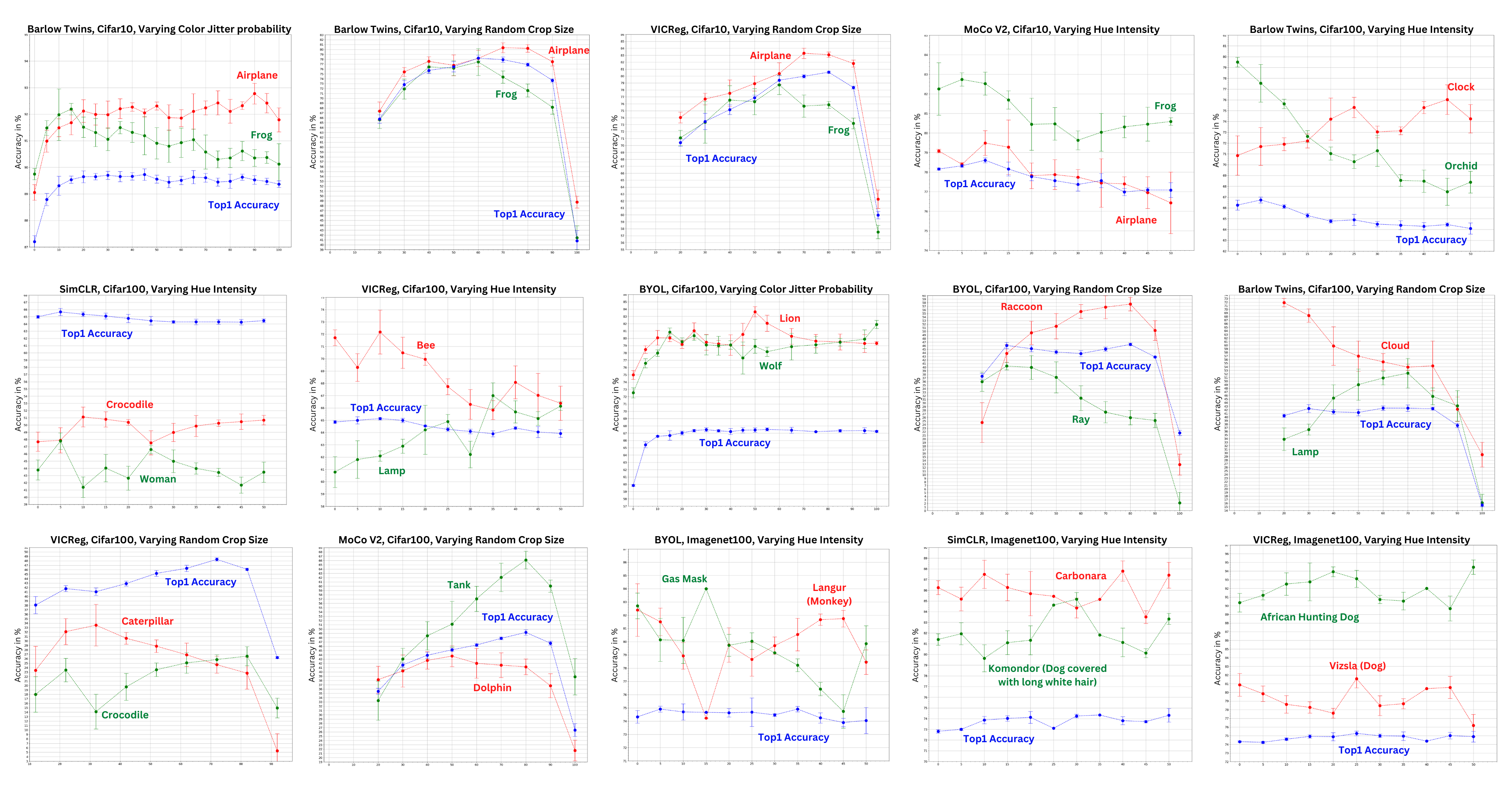
As depicted in Figure 2, we observe minimal fluctuation in the overall accuracy of each model as we slightly alter any of the transformations examined. This stands in stark contrast to the class-level accuracies observed, in which we discern significant variation in the accuracy value for many classes, as we vary the parameters of transformations, hinting at a greater impact of variations in transformation parameters on the class-level. Through the same figure, it becomes apparent that a number of classes exhibit distinct, and at times, entirely antithetical behaviors to each other within certain ranges of a transformation parameter. In the context of the datasets under scrutiny, this engenders a bias in the conventional training process of models, which either randomly samples transformation parameters or relies on hyperparameter optimization on overall accuracy to determine optimal parameters. This bias manifests itself in the manner in which choosing specific transformation parameters would impose a penalty on certain classes while favoring others. This is demonstrated in Figure 2 by the variation in accuracy of the Caterpillar and Crocodile classes for a model trained using VICReg (Bardes et al., 2022a), as the crop size is varied. The reported accuracies reveal that a small crop size benefits the Caterpillar class, as it encourages the model to learn features specific to its texture, while the Crocodile class is negatively impacted in the same range. These results suggest that a given choice of transformation probability or intensity has a direct effect on class level accuracies that is not necessarily visible through overall accuracy.
In order to gain deeper understanding of the inter-class bias observed in our previous analysis, we aim to further investigate the extent to which this phenomenon impacts the performance of models trained with self-supervised learning techniques. By quantitatively assessing the correlation scores between class-level accuracies obtained under different transformation parameters, we aim to clearly and unequivocally measure the prevalence of this bias in self-supervised learning methods. More specifically, a negative correlation score between the accuracy of two classes in response to varying a given transformation would indicate opposing behaviors for those classes. Despite its limitations, such as the inability to quantify the extent of bias and the potential for bias to manifest in specific ranges while remaining positively correlated in others (See Lion/Wolf pair in Figure 2), making it difficult to detect, this measure can still provide a preliminary understanding of the degree of inter-class bias. To this end, we conduct a series of experiments utilizing a ResNet encoder on the benchmark datasets of Cifar10 and Cifar100 (Krizhevsky, 2009). We employ a diverse set of state-of-the-art self-supervised approaches: Barlow Twins (Zbontar et al., 2021), MoCov2 (Chen et al., 2020b), BYOL (Grill et al., 2020), SimCLR (Chen et al., 2020a), and VICReg (Bardes et al., 2022a), and use the same fixed set of transformations as in our previous analysis depicted in Figure 2. We systematically vary the intensity of the hue, the probability of color jitter, the size of the random crop, and the probability of horizontal inversion through 20 uniformly sampled values for each, and repeat each training five times with distinct seed values. We compute the Pearson, Kendall and Spearman correlation coefficients for each pair of classes with respect to a given transformation parameter, as well as their respective p-values, and define class pairs with opposite behaviors as those with at least one negative correlation score of the three measured correlations lower than -0.3 and a p-value lower than 0.05. We then measure the ratio of classes with at least one opposite behavior to another class, compared to the total number of classes, in order to understand the extent of inter-class bias for a given transformation, method, and dataset.
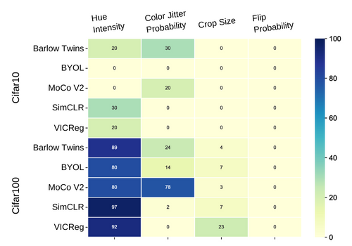
Our findings, as represented in Figure 3, indicate that the extent of inter-class bias for the self-supervised learning methods of interest varies among different transformations. This variability is primarily due to the fact that while these transformations aim to preserve the features that define a class across the original image and its transformed versions, they can also inadvertently compromise information specific to a particular class, while favoring the information of another class. It is noteworthy that for Cifar100, which comprises a vast array of natural image classes, we observe a considerable number of classes that exhibit inter-class bias when manipulating hue intensity. This is most likely a consequence of the high degree of overlap between classes when altering the colors within each class. Therefore, the selection of specific transformations and their associated parameters must be carefully tailored to the information that we aim to preserve within our classes, which constitutes a form of weak supervision in the choice of which classes to prioritize over others.
3.2 The choice of transformations directly affects downstream tasks
Examining the impact of transformations on downstream tasks, including variations in transformation parameters and compositions, is crucial for a complete understanding of their influence. To this end, we direct our investigation towards the representations that can be attained by training a VGG11 encoder architecture (Simonyan & Zisserman, 2015) with a MoCo v2 approach (Chen et al., 2020b) on the MNIST benchmark dataset (LeCun et al., 1998). Our study delves into the effects of different sets of compositions on the nature of the information embedded within the representation and its correlation to downstream tasks. For each representation obtained, we conduct a K-Means clustering (Lloyd, 1982) with ten clusters, and a linear evaluation utilizing the digit labels. In order to measure the efficacy of the clustering, we employ the Silhouette score (Rousseeuw, 1987) to assess the quality of the distribution of data within and between clusters without the use of labels. Additionally, we use the Adjusted Mutual Information score (AMI) (Vinh et al., 2010), which is a modified Mutual Information score that mitigates the influence of chance in clustering evaluations in comparison to clustering accuracy (Kuhn, 1955), by determining the level of agreement between the groupings of each cluster and the groupings of the classes in the ground truth. A more in-depth examination of the AMI score can be found in Supplementary materials, Section B.3.
| Transformation sets | Silhouette | AMI | Top1 Acc |
|---|---|---|---|
| First Set | 0.87 0.03 | 0.83 0.02 | 99.6 0.21 |
| Second Set | 0.66 0.08 | 0.37 0.06 | 62.1 2.94 |
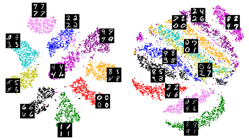
For our trainings, we employ two sets of transformations. The first set, comprised of padding, color inversion, rotation, and random cropping, aims to maximize the intra-class overlap of digits. The second set, which includes vertical flips, rotation, random cropping, and random erasing, is utilized to investigate the representation resulting from the destruction of digit information. Each training iteration is repeated five times with distinct seeds, and the average of their scores is computed. As depicted in Table 1, there is a decrease in both the AMI score and the top1 accuracy score for the training with the second set of transformations compared to the first set. This is to be expected as the second set of transformations is highly destructive to the digit information, resulting in a decline in performance that cannot be fully remedied, even with the supervised training used in linear evaluation. However, we observe that there is a slight decrease in the silhouette score compared to the decrease in the AMI score, with the score indicating that the clusters achieved from the representations of the second set of transformations are well-separated. As demonstrated in Figure 1, the clusters resulting from the two representations are distinguishable. The clusters resulting from the second set of transformations encapsulate handwriting information, such as line thickness and writing flow, forming handwriting classes for which the transformations maximized the intra-class overlap and minimized the inter-class overlap. This experiment implies that we can selectively supervise the specific image features that we aim to distinguish through a deliberate or unconscious selection of the transformations used during training, which would enhance the performance of the trained model for the associated downstream task.
3.3 The relevance of transformations is domain dependant
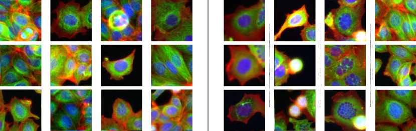
With the objective of exploring the amplitude of the effect of transformations on other domains, we perform experiments on microscopy images of cells under two conditions (untreated vs treated with a compound) available from BBBC021v1 (Caie et al., 2010), a dataset from the Broad Bioimage Benchmark Collection (Ljosa et al., 2012). Cells in their natural state can vary widely in appearance even when in the same condition, offering a more challenging context for SSRL (Figure 4). In order to observe the effect of transformations in such a domain, we preprocess these microscopy images by detecting all cell nuclei and extracting an 196x196 pixels image around each of them. We focus our study on three main compounds : Nocodazole, Cytochalasin B and Taxol. Technical details of the dataset used and the data preprocessing performed can be found in Supplementary Material A. We use a VGG13 (Simonyan & Zisserman, 2015) encoder architecture and MoCov2 (Chen et al., 2020b) as the self supervised approach, and run two separate trainings of the model from scratch for each compound, each of the two trainings with a different composition of transformations for invariance, repeated five times with distinct seeds. We then perform a K-Means (Lloyd, 1982) clustering (k=2) on the inferred test set embeddings and compute the Adjusted Mutual Information score (AMI) (Vinh et al., 2010) with respect to the ground truth compound labels of the compounds data subsets (untreated vs treated with Nocodazole, untreated vs treated with Cytochalasin B, untreated vs treated with Taxol).
| Nocodazole | Cytochalasin B | Taxol | |
|---|---|---|---|
| First Set | 0.190.01 | 0.270.02 | 0.160.05 |
| Second Set | 0.370.03 | 0.450.01 | 0.380.01 |
| Resnet101 | 0.39 | 0.57 | 0.43 |
For each composition of transformations explored, we repeat the training five times with different seeds, and compute the average and standard deviation of the AMI score (technical details of the the model training can be found in Supplementary material Section B.4). Table 2 displays the AMI scores achieved by using two different compositions of transformations in training, compared to the AMI score of a clustering on representations achieved with a pretrained Resnet101. By replacing slight random cropping and resizing, a transformation used in most existing self supervised approaches, with very strong random rotations of the image, we report a significantly higher mean AMI score, which shows that the model using random rotations is able to learn representations that better separate untreated from compound treated cells, including cells displaying subtle differences unnoticeable by the naked eye. Inversely, random cropping was destructive to the representations in this case, as the cropped images can miss out on relevant features in the sides of the cell. Compared to the slight effects of transformations reported on overall accuracy on Cifar10 and Imagenet100 in section 3.1, the significantly higher effect observed on this type of data suggests that transformations can have a higher impact on learning effective representations from images holding subtle differences between classes, and come to achieve similar performances to models pretrained with supervision.
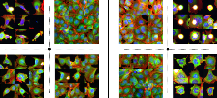
Beyond clustering into two conditions, we wonder what combination of transformations could lead to a proper clustering of cell phenotypes (or morphology). We explore different compositions of transformations in additional experiments with the same VGG13 (Simonyan & Zisserman, 2015) architecture and MoCov2 (Chen et al., 2020b) loss function. We then apply K-Means (Lloyd, 1982) clustering (k=4) on the representations obtained from the test set. As observed in Section 3.2, different compositions of transformations can lead to very different clustering results. This is further confirmed in the microscopy domain for Nocodazole (Figure 5), as we observe that the composition of color jitter, flips, rotation, affine, in addition to random crops, would result in clustering images by the number and size of cells, rather than by morphological features (Figure 5 left). We perform a training where affine transform and random crop were replaced by a center crop that preserves 50% of the image around the central cell. The latter resulted in four clusters where two out of the three cell phenotypes were detected. However, it also had the effect of splitting untreated cells into two different clusters (Figure 5 right). Altogether, engineering a combination of transformations represents a somewhat weak supervision that can become a silent bias or, alternatively, can be leveraged as a powerful tool to achieve a desirable result.
3.4 Improving representations requires a choice of transformations based on domain expertise
In the previous section, in order to achieve a clustering that extracts the three main cell morphologies produced by the Nocodazole treatment, we hypothesize that a focus on the center of the image (which is also necessarily the center of a cell given the preprocessing step), coupled with a focus on the relationship of the center cell to its surroundings were both necessary. We test this hypothesis by performing distinct trainings that combine both sets of transformations used in Figure 5 on the three compound data subsets : Nocodazole, Taxol and Cytochalasin B. Doing so produces some incompatible combinations of transformations, for instance, it brings together a random crop followed by a center crop, we keep both compositions separated in two independent Mocov2 losses. We then train a model to minimize the weighted sum of these two losses on each of the compound data subsets, and perform a K-Means clustering (k=4) on the resulting representations for the Nocodazole and Taxol subsets, and a K-Means clustering (k=2) on the resulting representation for the Cytochalasin B subset.
| Nocodazole | Cytochalasin B | Taxol | |
|---|---|---|---|
| Ours | 0.51 | 0.66 | 0.52 |
| Resnet101 | 0.39 | 0.57 | 0.43 |
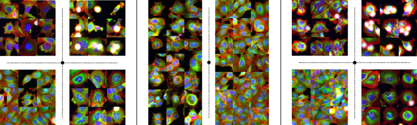
In the subsequent results in Figure 6 we can observe that we successfully separate all cell phenotypes obtained after each of the three compound treatments, from each other and from untreated cells, which validates our hypothesis. By performing another K-Means (k=2) on the same representations, we also report AMI scores for the task of separating the compound-treated cells from untreated cells, that can be considered quite high in this context where treated cells can look like untreated cells, vastly surpassing previous trainings with separate compositions of transformations in Table 3, as well as surpassing the performance of pretrained models. This suggests that more complex transformation manipulations, beyond modifying a single transformation parameter, can yield a better representation that significantly improves results on some specific tasks. However, identifying the right combination definitely requires domain expertise.
4 Conclusion
In this work, we performed experiments showing the impact of the choice, amplitude and combination of the transformations on the effectiveness of the self supervised representation that is learnt. We showed that the choice of transformation induces an inter-class bias but can also strongly affect other downstream tasks such as clustering, leading to unexpected results. We also demonstrated that the consequence of the choice of transformations can be very amplified in other domains where the difference between class is fuzzy or less visually identifiable. Altogether, some of the results can be understood somewhat intuitively. If one erases color from a car dataset, a deep network might not find enough correlated information to be able to classify cars on the basis of their original color. Thus the question: what is a good representation? The correct answer is that it depends on the downstream task. While it is what originally SSRL aimed to avoid, we showed, nonetheless, that choosing a rightful combination of transformations assembled in a non straightforward way by a domain expert can lead to very effective results.
5 Acknowledgments
This work was supported by ANR–10–LABX–54 MEMOLIFE and ANR–10 IDEX 0001–02 PSL* Université Paris and was granted access to the HPC resources of IDRIS under the allocation 2020-AD011011495 made by GENCI.
References
- Abnar et al. (2022) Abnar, S., Dehghani, M., Neyshabur, B., and Sedghi, H. Exploring the limits of large scale pre-training. In ICLR, 2022.
- Balestriero et al. (2022) Balestriero, R., Bottou, L., and LeCun, Y. The effects of regularization and data augmentation are class dependent. In NeurIPS, 2022.
- Bardes et al. (2022a) Bardes, A., Ponce, J., and LeCun, Y. Vicreg: Variance-invariance-covariance regularization for self-supervised learning. In ICLR, 2022a.
- Bardes et al. (2022b) Bardes, A., Ponce, J., and LeCun, Y. Vicregl: Self-supervised-learning of local visual features. In NeurIPS, 2022b.
- Bourou et al. (2023) Bourou, A., Daupin, K., Dubreuil, V., Thonel, A. D., Lallemand-Mezger, V., and Genovesio, A. Unpaired image-to-image translation with limited data to reveal subtle phenotypes. In ISBI, 2023.
- Caie et al. (2010) Caie, P. D., Walls, R. E., Ingleston-Orme, A., Daya, S., Houslay, T., Eagle, R., Roberts, M. E., and Carragher, N. O. High-Content Phenotypic Profiling of Drug Response Signatures across Distinct Cancer Cells. Molecular Cancer Therapeutics, 9:1913–1926, 2010.
- Caron et al. (2018) Caron, M., Bojanowski, P., Joulin, A., and Douze, M. Deep clustering for unsupervised learning of visual features. In ECCV, 2018.
- Caron et al. (2020) Caron, M., Misra, I., Mairal, J., Goyal, P., Bojanowski, P., and Joulin, A. Unsupervised learning of visual features by contrasting cluster assignments. In NeurIPS, 2020.
- Caron et al. (2021) Caron, M., Touvron, H., Misra, I., Jégou, H., Mairal, J., Bojanowski, P., and Joulin, A. Emerging properties in self-supervised vision transformers. In ICCV, 2021.
- Chen et al. (2020a) Chen, T., Kornblith, S., Norouzi, M., and Hinton, G. A simple framework for contrastive learning of visual representations. In ICML, 2020a.
- Chen & He (2021) Chen, X. and He, K. Exploring simple siamese representation learning. In CVPR, 2021.
- Chen et al. (2020b) Chen, X., Fan, H., Girshick, R., and He, K. Improved baselines with momentum contrastive learning, 2020b.
- Chen et al. (2021) Chen, X., Xie, S., and He, K. An empirical study of training self-supervised vision transformers. In ICCV, 2021.
- Coates et al. (2011) Coates, A., Ng, A., and Lee, H. An analysis of single-layer networks in unsupervised feature learning. In The International Conference on Artificial Intelligence and Statistics, 2011.
- Cubuk et al. (2019) Cubuk, E. D., Zoph, B., Mane, D., Vasudevan, V., and Le, Q. V. Autoaugment: Learning augmentation policies from data. In CVPR, 2019.
- Deng et al. (2009) Deng, J., Dong, W., Socher, R., Li, L.-J., Li, K., and Fei-Fei, L. Imagenet: A large-scale hierarchical image database. In 2009 IEEE conference on computer vision and pattern recognition, pp. 248–255. Ieee, 2009.
- Dwibedi et al. (2021) Dwibedi, D., Aytar, Y., Tompson, J., Sermanet, P., and Zisserman, A. With a little help from my friends: Nearest-neighbor contrastive learning of visual representations. ICCV, 2021.
- Ermolov et al. (2021) Ermolov, A., Siarohin, A., Sangineto, E., and Sebe, N. Whitening for self-supervised representation learning. In ICML, 2021.
- Geirhos et al. (2020) Geirhos, R., Jacobsen, J.-H., Michaelis, C., Zemel, R., Brendel, W., Bethge, M., and Wichmann, F. A. Shortcut learning in deep neural networks. Nature Machine Intelligence, 2(11):665–673, nov 2020. doi: 10.1038/s42256-020-00257-z.
- Grill et al. (2020) Grill, J.-B., Strub, F., Altché, F., Tallec, C., Richemond, P., Buchatskaya, E., Doersch, C., Avila Pires, B., Guo, Z., Gheshlaghi Azar, M., Piot, B., kavukcuoglu, k., Munos, R., and Valko, M. Bootstrap your own latent - a new approach to self-supervised learning. In NeurIPS, 2020.
- Huang et al. (2021) Huang, W., Yi, M., and Zhao, X. Towards the generalization of contrastive self-supervised learning, 2021.
- Krizhevsky (2009) Krizhevsky, A. Learning multiple layers of features from tiny images. 2009.
- Kuhn (1955) Kuhn, H. W. The hungarian method for the assignment problem. Naval Research Logistics Quarterly, 2(1-2):83–97, 1955.
- Lamiable et al. (2022) Lamiable, A., Champetier, T., Leonardi, F., Cohen, E., Sommer, P., Hardy, D., Argy, N., Massougbodji, A., Del Nery, E., Cottrell, G., Kwon, Y.-J., and Genovesio, A. Revealing invisible cell phenotypes with conditional generative modeling. 2022.
- LeCun et al. (1998) LeCun, Y., Cortes, C., and Burges, C. J. The mnist database of handwritten digits, 1998.
- Lee & Aune (2021) Lee, D. and Aune, E. Computer vision self-supervised learning methods on time series, 2021.
- Li et al. (2020) Li, Y., Hu, G., Wang, Y., Hospedales, T., Robertson, N. M., and Yang, Y. Dada: Differentiable automatic data augmentation. In ECCV, 2020.
- Li et al. (2022) Li, Z., Chen, Y., LeCun, Y., and Sommer, F. T. Neural manifold clustering and embedding, 2022.
- Liu et al. (2021) Liu, A., Huang, Z., Huang, Z., and Wang, N. Direct differentiable augmentation search. In ICCV, 2021.
- Ljosa et al. (2012) Ljosa, V., Sokolnicki, K. L., and Carpenter, A. E. Annotated high-throughput microscopy image sets for validation. Nature Methods, 9:637–637, 2012.
- Lloyd (1982) Lloyd, S. Least squares quantization in pcm. IEEE Transactions on Information Theory, 28:129–137, 1982.
- Masud et al. (2022) Masud, U., Cohen, E., Bendidi, I., Bollot, G., and Genovesio, A. Comparison of semi-supervised learning methods for high content screening quality control. In ECCV 2022 BIM Workshop, 2022.
- Pal et al. (2020) Pal, D. K., Nallamothu, S., and Savvides, M. Towards a hypothesis on visual transformation based self-supervision. In British Machine Vision Conference, 2020.
- Patrick et al. (2021) Patrick, M., Asano, Y. M., Kuznetsova, P., Fong, R., Henriques, J. F., Zweig, G., and Vedaldi, A. On compositions of transformations in contrastive self-supervised learning. In ICCV, 2021.
- Perakis et al. (2021) Perakis, A., Gorji, A., Jain, S., Chaitanya, K., Rizza, S., and Konukoglu, E. Contrastive learning of single-cell phenotypic representations for treatment classification. In Machine Learning in Medical Imaging, pp. 565–575. 2021.
- Reed et al. (2021) Reed, C. J., Metzger, S., Srinivas, A., Darrell, T., and Keutzer, K. Selfaugment: Automatic augmentation policies for self-supervised learning. In CVPR, 2021.
- Rousseeuw (1987) Rousseeuw, P. J. Silhouettes: A graphical aid to the interpretation and validation of cluster analysis. Journal of Computational and Applied Mathematics, 20:53–65, 1987.
- Ruppli et al. (2022) Ruppli, C., Gori, P., Ardon, R., and Bloch, I. Optimizing transformations for contrastive learning in a differentiable framework. In MICCAI MILLanD workshop, 2022.
- Saunshi et al. (2019) Saunshi, N., Plevrakis, O., Arora, S., Khodak, M., and Khandeparkar, H. A theoretical analysis of contrastive unsupervised representation learning. In ICML, 2019.
- Saunshi et al. (2022) Saunshi, N., Ash, J. T., Goel, S., Misra, D., Zhang, C., Arora, S., Kakade, S. M., and Krishnamurthy, A. Understanding contrastive learning requires incorporating inductive biases. CoRR, 2022.
- Simonyan & Zisserman (2015) Simonyan, K. and Zisserman, A. Very deep convolutional networks for large-scale image recognition. In ICLR, 2015.
- Vinh et al. (2010) Vinh, N. X., Epps, J., and Bailey, J. Information theoretic measures for clusterings comparison: Variants, properties, normalization and correction for chance. Journal of Machine Learning Research, 11:2837–2854, 2010.
- von Kügelgen et al. (2021) von Kügelgen, J., Sharma, Y., Gresele, L., Brendel, W., Schölkopf, B., Besserve, M., and Locatello, F. Self-supervised learning with data augmentations provably isolates content from style. In NeurIPS, 2021.
- Wagner et al. (2022) Wagner, D., Ferreira, F., Stoll, D., Schirrmeister, R. T., Müller, S., and Hutter, F. On the importance of hyperparameters and data augmentation for self-supervised learning. CoRR, 2022.
- Wang & Isola (2020) Wang, T. and Isola, P. Understanding contrastive representation learning through alignment and uniformity on the hypersphere. In ICML, 2020.
- Wang & Qi (2021) Wang, X. and Qi, G.-J. Contrastive learning with stronger augmentations, 2021.
- Wen & Li (2021) Wen, Z. and Li, Y. Toward understanding the feature learning process of self-supervised contrastive learning. In ICML, 2021.
- Xiao et al. (2021) Xiao, T., Wang, X., Efros, A. A., and Darrell, T. What should not be contrastive in contrastive learning. In ICLR, 2021.
- Yang et al. (2021) Yang, S., Das, D., Chang, S., Yun, S., and Porikli, F. Distribution estimation to automate transformation policies for self-supervision. In NeurIPS Workshop: Self-Supervised Learning - Theory and Practice, 2021.
- Yeh et al. (2022) Yeh, C.-H., Hong, C.-Y., Hsu, Y.-C., Liu, T.-L., Chen, Y., and LeCun, Y. Decoupled contrastive learning. In ECCV, 2022.
- Zbontar et al. (2021) Zbontar, J., Jing, L., Misra, I., LeCun, Y., and Deny, S. Barlow twins: Self-supervised learning via redundancy reduction. In ICML, 2021.
- Zhang & Ma (2022) Zhang, J. and Ma, K. Rethinking the augmentation module in contrastive learning: Learning hierarchical augmentation invariance with expanded views. CVPR, 2022.
- Zheng et al. (2021) Zheng, M., You, S., Wang, F., Qian, C., Zhang, C., Wang, X., and Xu, C. Ressl: Relational self-supervised learning with weak augmentation. NeurIPS, 2021.
Appendix A Datasets
We perform the experiments mentioned in Section 3.3 on microscopy images available from BBBC021v1 (Caie et al., 2010), a dataset from the Broad Bioimage Benchmark Collection (Ljosa et al., 2012). This dataset is composed of breast cancer cells treated for 24 hours with 113 small molecules at eight concentrations, with the top concentration being different for many of the compounds through a selection from the literature. Throughout the quality control process, images containing artifacts or with out of focus cells were deleted, and the final dataset totalled into 13,200 fields of view, imaged in three channels, each field composed of thousands of cells. In the cells making up the dataset, twelve different primary morphological reactions from the compound-concentrations were identified, with only six identified visually, while the remainder were defined based on the literature, as the differences between some morphological reactions were very subtle. We perform a simple cell detection in each field of view, in order to crop cells centered in (196x196px) images. We then filter the images by compound-concentration, and keep images treated by Nocodazole at its 4 highest concentrations. These compound-concentrations result in 4 morphological cell reactions, for which we don’t have individual labels for each cell image. We sample the same number of images from views of untreated cells, totalling into a final data subset of 3500 images, which we split into 70% training data, 10% validation data and 20% test data. We repeat the same process for the compounds Taxol and Cytochalasin B, each containing 4 and 2 morphological reactions respectively, to result in data subsets of sizes 1900 and 2300 images, respectively.
Appendix B Model training
B.1 Study of inter-class bias in self supervised classification
For results in Section 3.1 and Table 4, we run several trainings of 12 SSRL methods (Bardes et al., 2022a; Caron et al., 2018, 2020; Chen et al., 2020a; Chen & He, 2021; Chen et al., 2020b; Dwibedi et al., 2021; Grill et al., 2020; Lee & Aune, 2021; Zbontar et al., 2021; Zheng et al., 2021) on Cifar10 and Cifar100 (Krizhevsky, 2009) with a Resnet18 architecture, with a pretraining of 1000 epochs without labels. We use the same transformations with similar parameters on all approaches, namely a 0.4 maximal brightness intensity, 0.4 maximum contrast intensity, 0.2 maximum saturation intensity, all with a fixed probability of 80%. With a maximal hue intensity of 0.5, we vary the hue probability of application between 0% and 100% by uniformly sampling 20 probability values in this range. We use stochastic gradient descent as optimization strategy for all approaches, and through a line search hyperparameter optimization, we use a batch size of 512 for all approaches except Dino (Caron et al., 2021) and Vicreg (Bardes et al., 2022a) for which we use a batch size of 256. Following the hyperparameters used in the literature of each approach, we use a projector with a 256 output dimension for most methods, except for Barlow Twins (Zbontar et al., 2021), Simsiam (Chen & He, 2021), Vicreg (Bardes et al., 2022a) and Vibcreg (Lee & Aune, 2021), for which we use a projector with a 2048 output dimension, and DeepclusterV2 (Caron et al., 2018) and Swav (Caron et al., 2020) for which we use a projector with a 128 output dimension. For some momentum based methods (Byol (Grill et al., 2020), MocoV2+ (Chen et al., 2020b), NNbyol (Dwibedi et al., 2021) and Ressl (Zheng et al., 2021)), we use a base Tau momentum of 0.99 and use a base Tau momentum of 0.9995 for Dino (Caron et al., 2021). For Mocov2+ (Chen et al., 2020b), NNCLR (Dwibedi et al., 2021) and SimCLR (Chen et al., 2020a), we use a temperature of 0.2.
We train the Barlow Twins (Zbontar et al., 2021) based model with a learning rate of 0.3 and a weight decay of , and Byol (Grill et al., 2020) as well as NNByol (Dwibedi et al., 2021) with a learning rate of 1.0 and a weight decay of . We train DeepclusterV2 (Caron et al., 2018) with a learning rate of 0.6, 11 warmup epochs, a weight decay of , and 3000 prototypes. We train Dino with a learning rate of 0.3, a weight decay of , and 4096 prototypes, while we train MocoV2+ (Chen et al., 2020b) with a learning rate of 0.3, a weight decay of and a queue size of 32768. For NNclr (Dwibedi et al., 2021), we use a learning rate of 0.4, a weight decay of , and a queue size of 65536. We train ReSSL (Zheng et al., 2021) with a learning rate of 0.05, and a weight decay of , while we train SimCLR (Chen et al., 2020a) with a learning rate of 0.4, and a weight decay of . For Simsiam (Caron et al., 2020), we use a learning rate of 0.5, and a weight decay of , and use for Swav (Caron et al., 2020) a learning rate of 0.6, a weight decay of , a queue size of 3840, and 3000 prototypes. We use for Vicreg (Bardes et al., 2022a) and Vibcreg (Lee & Aune, 2021) a learning rate of 0.3, a weight decay of , an invariance loss coefficient of 25, and a variance loss coefficient of 25. We use a covariance loss coefficient of 1.0 for Vicreg (Bardes et al., 2022a) and a covariance loss coefficient of 200 for Vibcreg (Lee & Aune, 2021). We perform linear evaluation after each pretraining for all methods, through freezing the weights of the encoder and training a classifier for 100 epochs. We use 5 different global seeds (5, 6, 7, 8, 9) for each hue intensity value, and compute the mean top1 accuracy resulting from the linear evaluation, using each of the 5 different experiences. Each training run was made on a single V100 GPU. On ImageNet100 (Deng et al., 2009), we train a Resnet18 encoder with BYOL (Grill et al., 2020), MoCo V2 (Chen et al., 2020b), VICReg (Bardes et al., 2022a) and SimCLR (Chen et al., 2020a), using a batch size of 128 for 400 epochs. We use a learning rate of 0.3 and a weight decay of for MoCo V2 and VICReg, and a weight decay of and learning rates of 0.4 and 0.45 for SimCLR and BYOL respectively. We repeat each experience three times with three global seeds (5,6 and 7) and compute its mean and standard deviation.
For the results in Figures 2 and 2, we reuse the same training hyperparameters for Barlow Twins (Zbontar et al., 2021), Moco V2 (Chen et al., 2020b), BYOL (Grill et al., 2020), SimCLR (Chen et al., 2020a) and Vicreg (Bardes et al., 2022a), and uniformly sample 10 values in the range of [0;0.5] for the maximal hue intensity, with a fixed 80% probability. We run different experiments for the 5 global seeds for each hue intensity, and compute their mean and standard deviation. We perform the same process while fixing maximal hue intensity to 0.1, and varying its probability by uniformly sampling 20 probability values in the range [0;100]. We repeat a similar process for the random cropping and horizontal flips, by sampling 8 values uniformly in the range of [20;100] of the size ratio to keep of the image, and sampling 20 values uniformly in the range of [0;100] for the probability of application of horizontal flips.
B.2 MNIST Clustering
For the displayed clustering results in Figure 1, we use a VGG11 (Simonyan & Zisserman, 2015) architecture, with a projector of 128 output dimension, trained using a MocoV2+ (Chen et al., 2020b) loss function on Mnist (LeCun et al., 1998) for 250 epochs. We use an Adam optimizer, a queue size of 1024, and a batch size of 32. We set temperature at 0.07, learning rate at 0.001, and weight decay at 0.0001. We run two trainings with two separate sets of compositions of transformations, each run on a single V100 GPU, and perform a Kmeans (K=10) clustering on the resulting representations of the test set. For the digit clustering, we use a composition of transformations composed of a padding of 10% to 40% of the image size, color inversion, rotation with a maximal angle of 25°, and random crop with a scale in the range of [0.5;0.9] of the image, and then a resizing of the image to 32x32 pixels. For the handwriting flow clustering, we use a composition of transformations composed of horizontal & vertical flips with an application probability of 50% each, rotations with a maximal angle of 180°, random crop with a scale in the range of [0.9;1.1], and random erasing of patches of the image, with a scale in the range of [0.02;0.3] of the image and a probability of 50%. We perform linear evaluation by training classifiers on the frozen representations of the trained models, in order to predict the digit class, and evaluate using the top1 accuracy score.
B.3 Clustering evaluation with the AMI Score
We use the adjusted mutual information (AMI) (Vinh et al., 2010) in Sections 3.3 and 3.4 to evaluate clustering quality, and to measure the similarity between two clusterings. It is a value that ranges from 0 to 1, where a higher value indicates a higher degree of similarity between the two clusterings. This score holds an advantage over clustering accuracy (Kuhn, 1955) in one main aspect, being that the clustering accuracy only measures how well the clusters match the labels of the true clusters, and does not take into account the structure within the clusters, such as heterogeneity of some of the clusters. This is unlike the AMI score, which takes into account both the structure between the clusters and the structure within the clusters, by measuring the ”agreement” between the groupings of a predicted cluster and the groupings of the true cluster. If both clusterings agree on most of the groupings, then the AMI score will be high, and inversely low if they do not.
The AMI score can be computed with the formula :
Where is the mutual information between the two clusterings, is the expected mutual information between the two clusterings, is the entropy of the clustering , and is the entropy of the clustering . Mutual information (MI) is a measure of the amount of information that one variable contains about another variable. In the context of AMI, the two variables are the clusterings and . is a measure of to what extent the two clusterings are related to each other. Entropy is a measure of the amount of uncertainty in a random variable. In the context of AMI, the entropy of a clustering ( or ) is a measure of how much uncertainty exists within the clustering. Expected mutual information () is the average mutual information between the two clusterings, assuming that the two clusterings are independent.
The adjusted mutual information (AMI) is calculated by first subtracting the expected mutual information () from the actual mutual information (). This results in a measure of of the extent of the relationship between the two clusterings beyond what would be expected by chance. This value is then divided by the difference between the maximum possible entropy () and the expected mutual information (). Normalization of the result is achieved through this process, ensuring that it is always between 0 and 1. Figure 7 shows the results of a clustering achieved on Nocodazole vs untreated cells, with the AMI score computed after randomisation of the ground truth labels, in contrast to clustering results achieved without randomizing the labels.
B.4 Cellular Clustering
For the results in Sections 3.3, 3.4, we use a VGG13 (Simonyan & Zisserman, 2015) architecture, trained using a MocoV2+ (Chen et al., 2020b) loss function on the data subsets of the microscopy images available from BBBC021v1 (Caie et al., 2010), presented in Section A, with a batch size of 128, for 400 epoch. We use an Adam optimizer, a queue size of 1024, and set temperature at 0.07, learning rate at 0.001, and weight decay at 0.0001. Each training is made on a single V100 GPU. We perform a Kmeans (K=2) on the resulting representations of the test set of the data subsets of Nocodazole, Cytochalasin B and Taxol, and evaluate the quality of the achieved clusters compared to the ground truth using the AMI score (Vinh et al., 2010).
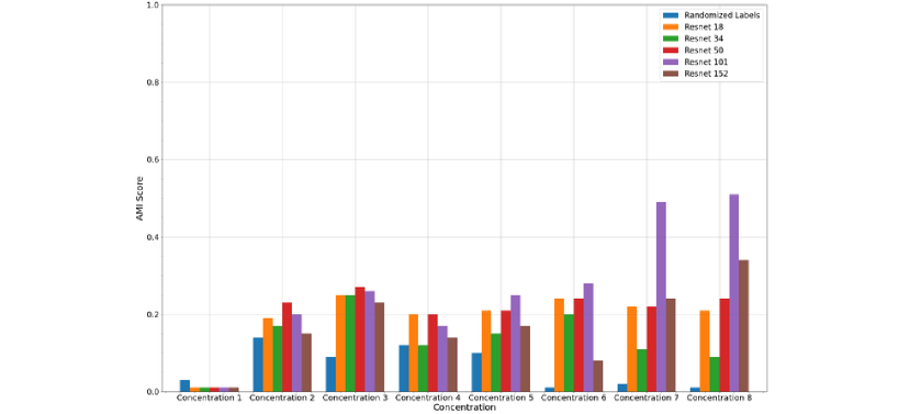
In Table 2, we achieve the first AMI result through usage of an affine transformation composed of a rotation with an angle of 20°, a translation of 0.1 and a shear with a 10° angle, coupled with color jitter with a brightness, contrast and saturation intensity of 0.4, and a hue intensity of 0.125, with a 100% probability, as well as random cropping of the image with a scale in the range of [0.9;1.1] and resizing to original image size of 196x196 pixel. For the second row result, we use an affine transformation composed of a rotation with an angle of 20°, a translation of 0.1 and a shear with a 10° angle, coupled with color jitter with a brightness, contrast and saturation intensity of 0.4, and a hue intensity of 0.125, with a 100% probability, and a random rotation with a maximal angle of 360°. The results achieved through a Resnet101, are achieved by performing a Kmeans (K=2) on the representations achieved on the compound subsets using the Resnet101, and evaluating the cluster assignment quality compared to ground truth using the AMI score (Vinh et al., 2010). The choice of Resnet101 over other Resnet sizes is motivated through testing the performance of different sizes of Resnets on the different concentrations of Nocadozole/untreated cells, on which Resnet101 consistently shows the highest performance on the 4 highest concentrations, as shown in Figure 7.
For the clusterings in Figure 5, we train the same architecture with the same hyperparameters on different compositions of transformations, and perform a Kmeans (K=4) on the resulting representations of the test set. For all the clusters, the images displayed are the images closest to the centroïd of each cluster using an euclidean distance. The clustering in Figure 5 left is achieved by using a composition of color jitter with a brightness, contrast and saturation intensity of 0.4, and a hue intensity of 0.125, with a 100% probability, and horizontal and vertical flips, each with 50% probability of application, as well as random rotations with a maximal angle of 360°, an affine transformation composed of a rotation with an angle of 20°, a translation of 0.1 and a shear with a 10° angle, and a random crop with a scale sampled in the range [0.9;1.1], followed by a resizing of the image to the original size. The clustering in Figure 5 right is achieved by color jitter with a brightness, contrast and saturation intensity of 0.4, and a hue intensity of 0.125, with a 100% probability, horizontal and vertical flips, each with 50% probability of application, random rotations with a maximal angle of 360°, and a center crop with a scale of 0.5, followed by a resizing of the image to the original size. For the clustering in Figure 6, we trained the model with a sum of the losses (and corresponding transformations) of the models used in Figure 5. Through a gridsearch hyperparameter optimization, with the goal of optimizing the AMI score of a Kmeans clustering (K=2), we attributed a coefficient of 0.4 to the loss of the model used in Figure 5 left, and a coefficient of 1.0 to the loss of the model used in Figure 5 right.
Appendix C Additional inter-class bias results
| Barlow Twins | Byol | Deep Cluster v2 | MoCo V2+ | nnByol | nnclr | Ressl | SimCLR | SimSiam | SwaV | Vibcreg | Vicreg | |
| Mean | 89.59 | 92.09 | 86.9 | 92.37 | 91.3 | 89.76 | 90.21 | 90.16 | 89.6 | 86.96 | 82.47 | 89.82 |
| Std | 0.73 | 0.37 | 1.9 | 0.44 | 0.57 | 0.74 | 0.85 | 0.87 | 1.01 | 1.2 | 0.89 | 0.94 |