Quantum Spin Supersolid as a precursory Dirac Spin Liquid
in a Triangular Lattice Antiferromagnet

Abstract

Based on the idea that the Dirac spin liquid is the parent state for numerous competing orders, we propose the triangular lattice antiferromagnet Na₂BaCo(PO₄)₂, which exhibits a quantum spin supersolid, to be a precursory Dirac spin liquid. Despite the presence of a three-sublattice magnetic order resembling a spin “supersolid”, we suggest that this system is close to a Dirac spin liquid by exploring its spectroscopic response. The physical consequence is examined from the spectroscopic response, and we establish the continuous spectra near the M point in addition to the K point excitation from the spinon continuum on top of the three-sublattice order. This proposal offers a plausible understanding of the recent inelastic neutron scattering measurement in Na₂BaCo(PO₄)₂ and could inspire further research in relevant models and materials.

The duality has played an important role in the understanding of the strongly coupled models in statistical physics since the Kramers-Wannier duality for the Ising model Kramers and Wannier (1941). The modern charge-vortex duality allows the description of novel phases and phase transitions such as superfluid-Mott transition and the vortex phases of bosons or Cooper pairs Fisher and Lee (1989); Fisher (2004); Balents et al. (1999, 2005); Karch and Tong (2016) from the dual vortices, which could be cumbersome with the original charge language. The fermion version of the charge-vortex duality has important applications in the composite fermion for the half-filled Landau level and the surface fermions of U(1) spin liquids in 3D Son (2015); Wang and Senthil (2016). More recently, the idea of boson-fermion duality has been applied to the deconfined quantum criticality. The well-known Néel-VBS (valence bond solid) transition that is believed to have a deconfined quantum criticality and is then described by the non-compact CP¹ model (NCCP¹) with the fractionalized bosonic spinons coupled to a non-compact U(1) gauge field. It was argued that Wang et al. (2017), the NCCP¹ theory is dual to two massless Dirac fermions coupled with a U(1) gauge field, i.e. ${N_{f}=2}$ quantum electrodynamics (QED₃). Thinking reversely from the emergent QED₃ that is the description for the U(1) Dirac spin liquid (DSL) Song et al. (2019), Ref. Song et al., 2019 views the U(1) DSL as the mother state of the competing orders such as Néel and VBS in 2D by further studying the symmetry properties of the monopole operators and ensuring the concomitant of the ordering-driven spontaneous mass generation and the confinement. It clearly indicates the increased stability of the U(1) DSL on frustrated lattices Song et al. (2019). In this work, we attempt to identify the specific material and model that may reveal the signatures of DSL and competing orders on the triangular lattice.

We turn to the material’s side. It is the conventional belief that the $3d$ transition metal oxides should have more symmetric spin models. In reality, all the $3d$ transition metal ions have rather different physical properties, exhibiting rich behaviors with a diverse of models that depend sensitively on the structures and the crystal field environments Chen et al. (2009); Chen (2017); Li and Chen (2019); Su et al. (2019). In many cases, the orbitals get involved and wildly change the physics. For the Co ion, the often-discussed scenario is about the selection of the high or low spin states due to the competition between the Hund’s coupling and the crystal electric field splitting. More recently, the spin-orbit coupling of the Co ion has received quite some attention. This occurs when the electrons partially fill the $t_{2g}$ shell Witczak-Krempa et al. (2014). Due to the active spin-orbit coupling and the orbitals, the local moment of the relevant Co ion is no longer pure spins, and is instead an entangled mixture of spin and orbital. The resulting effective model is often anisotropic instead of Heisenberg-like. The well-known limiting examples were the quasi-1D Ising magnets CoNb₂O₆, BaCo₂V₂O₈ and SrCo₂V₂O₈ Lee et al. (2010); Faure et al. (2018); Wang et al. (2015); Zou et al. (2021); Wang et al. (2018a, b). For the same reason, the Kitaev interaction has been extended to the honeycomb cobaltates including Na₂Co₂TeO₆ and Na₂Co₂SbO₆ Liu et al. (2020); Liu and Khaliullin (2018); Sano et al. (2018), and a similar form of Kitaev interaction is reinvoked for CoNb₂O₆ Morris et al. (2021); Ringler et al. (2022). We here consider the triangular lattice antiferromagnet Na₂BaCo(PO₄)₂ where the model is the spin-1/2 easy-axis XXZ model Sheng et al. (2022).

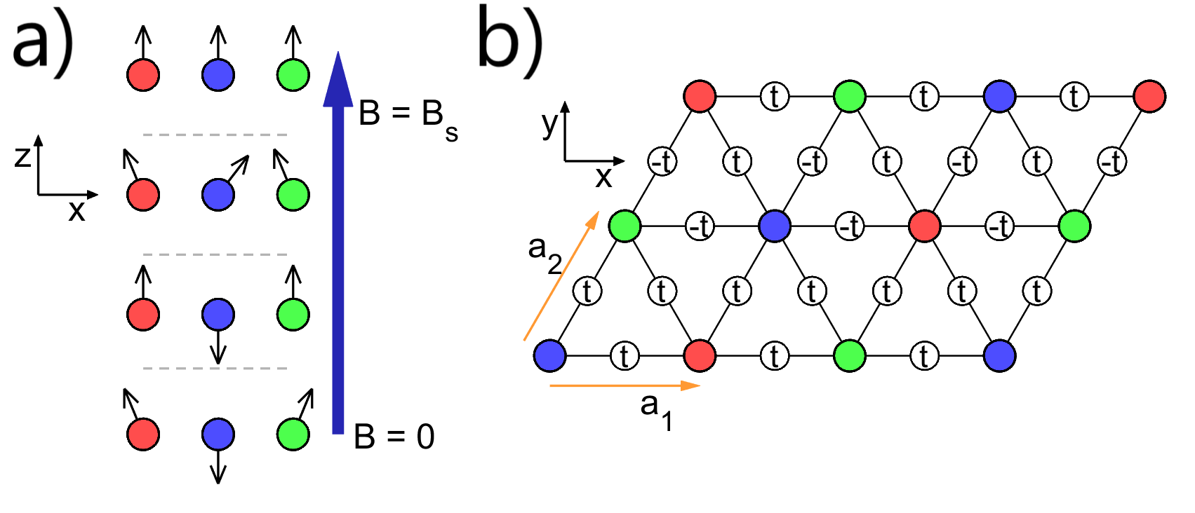
Figure 1: (a) The spin orientation of various magnetic phases for the easy-axis XXZ model on the triangular lattice. As the field ${{\mathbf{B}}=B\hat{z}}$ increases from zero, the system enters the 3-sublattice supersolid (Y-shape), UUD, V-shape and the fully polarized states. The sublattices are plotted in red, green and blue. (b) The spinon hoppings $t_{ij}$ are chosen with a gauge choice supporting a $\pi$ flux.

Na₂BaCo(PO₄)₂ develops a three-sublattice antiferromagnetic order below about 0.15K. The weak exchange couplings allow the external magnetic fields about 2T to polarize the spins for both in-plane and out-of-plane directions Li et al. (2020). The magnetic excitations of these polarized states are quantitatively captured by the linear spin-wave theory based on the spin-1/2 XXZ model with strong fields. The ratio of the coupling for the $xy$ components over the $z$-component coupling is ${\sim 0.58}$, and both are antiferromagnetic and thus fully-frustrated. The spin-1/2 XXZ model on the triangular lattice is a well-studied problem. The phase diagrams with and without the field are quite clear. The supersolid order, that breaks both the U(1) symmetry via the in-plane spin order and the lattice translation via the $z$-component order, was known to be present in the ferromagnetic $xy$ and the antiferromagnetic $z$ regime, and was later shown to persist to the fully-frustrated regime with both antiferromagnetic $xy$ and $z$ couplings until the Heisenberg point Yamamoto et al. (2014a); Wang et al. (2009) and is entirely due to quantum origin. Thus Na₂BaCo(PO₄)₂ develops a quantum supersolid antiferromagnetic order at low temperatures. Due to the U(1) symmetry and the easy-axis coupling, the intermediate field along the $z$ direction stabilizes a 1/3 magnetization plateau with a ‘UUD’ (“up-up-down”) spin configuration in Na₂BaCo(PO₄)₂. What is surprising is that, the zero-field excitation exhibits unusual continuous spectra at low energies near $\mathbf{M}$ point in the reciprocal space, besides $\mathbf{K}$ point excitations lsw . This is apparently inconsistent with the expected spin-wave excitation for the three-sublattice supersolid. This feature is absent for Ba₃CoSb₂O₉ that is also described by XXZ model but in an easy-plane anisotropy Ito et al. (2017); Ma et al. (2016). To understand the puzzling experiment in Na₂BaCo(PO₄)₂, we propose a probable explanation from the precursory U(1) DSL. Numerical simulations have found a wider region of U(1) DSL with the $J_{1}$-$J_{2}$ spin model on the triangular lattice than the square lattice Sherman et al. (2022); Ferrari and Becca (2019); Iqbal et al. (2016), supporting the increased stability of DSL on frustrated lattices Song et al. (2019). It was argued that Song et al. (2019), the triangular lattice spin-1/2 Heisenberg antiferromagnet might be proximate to the DSL such that the spin dynamics might carry the hint of Dirac spinons. The fully-frustrated XXZ model in the easy-axis regime is probably more frustrated than the nearest-neighbor Heisenberg model and the easy-plane XXZ model for Ba₃CoSb₂O₉, and is likely to be more proximate to the DSL. Here we attempt to understand the spin dynamics of Na₂BaCo(PO₄)₂ from the precursory DSL.

Model.—Na₂BaCo(PO₄)₂ is modeled as the spin-1/2 XXZ model on the triangular lattice with Zhong et al. (2019); Li et al. (2020),

$$H_{\text{XXZ}}=\sum_{\langle ij\rangle}J_{\perp}(S_{i}^{x}S_{j}^{x}+S_{i}^{y}S_{j}^{y})+J_{z}S_{i}^{z}S_{j}^{z}-B\sum_{i}S_{i}^{z},$$ (1)

where ${J_{\perp},J_{z}>0}$ are both antiferromagnetic and the last term is the Zeeman effect from an effective out-of-plane field $B$. For an easy-axis anisotropy ${0<J_{\perp}/J_{z}<1}$, one finds that the magnetic phase goes through Y-shape, UUD, and V-shape spin configurations with a ${\sqrt{3}\times\sqrt{3}}$ three-sublattice structure with increasing fields Yamamoto et al. (2014b), and eventually becomes a fully polarized state above a saturation field ${B_{s}={3}J_{xx}/2+3J_{z}}$. In Fig. 1, the spin orientation on each sublattice is depicted for different phases. In this work, we focus on the zero-field state, known as the spin supersolid Wessel and Troyer (2005); Melko et al. (2005). The spin-wave study based on the spin supersolid cannot produce the low-energy excitation near $\mathbf{M}$ points, indicating the insufficiency of the supersolid order for the spin dynamics.

Figure 2: (a) The spinon bands in MBZ with ${\tilde{J}_{z}=4.394t}$, $\tilde{J}_{\perp}=4.102t$, ${\mu=0}$. The weakly gapped Dirac cones are relevant for the low-energy INS signals. The bands below (above) the Fermi surface are painted in blue (red). The orange rectangle indicates the MBZ. (b) The spinon dispersion along the red dashed line in (a). (c) The hexagonal lattice Brillouin zone with high symmetry points. The orange rectangle is the MBZ.

We aim to phenomenologically find a state that contains the supersolid order and at the same time provides the continuous spectra near both K and M points. Based on the recent progress about the DSL and competing orders Song et al. (2019), we thus consider the possibility of precursory DSL for Na₂BaCo(PO₄)₂. To describe this state, we first use the Abrikosov fermion representation for the spin operator with ${{\bm{S}}_{i}=\frac{1}{2}f^{\dagger}_{i\alpha}{\bm{\sigma}}_{\alpha\beta}f_{i\beta}}$ and the Hilbert space constraint ${\sum_{\alpha}f_{i\alpha}^{\dagger}f_{i\alpha}=1}$, where $f_{i\alpha}^{\dagger}\ (f_{i\alpha})$ creates (annihilates) a fermionic spinon at the site $i$ with spin $\alpha$. Now the supersolid is present via the fermion bilinear in $\langle{\bm{S}}_{i}\rangle$, and the continuous spectra in the dynamic spin structure factor would be captured by the particle-hole continuum of the fermionic spinons at least at the mean-field level. To construct such a state and/or mainly the many-body wavefunction, we use the Weiss mean-field theory to incorporate the supersolid order and rely on the slave fermion mean-field theory to take care of the DSL. For the first one, one expresses $S^{\mu}_{i}S^{\mu}_{j}$ as $\langle S^{\mu}_{i}\rangle S^{\mu}_{j}$ where $\langle S^{\mu}_{i}\rangle$ works as the supersolid order. For the second one, we work on the triangular lattice $\pi$-flux DSL because it naturally gives the continuous excitations near the M point Shen et al. (2016). Combining these two points, we write down the following mean-field Hamiltonian for ${B=0}$,

$$\begin{split}H_{\text{MF}}&=\sum_{\langle ij\rangle\alpha}t_{ij}f_{i\alpha}^{\dagger}f_{j\alpha}-\mu\sum_{i\alpha}f_{i\alpha}^{\dagger}f_{i\alpha}\\ &+\sum_{\langle ij\rangle}\tilde{J}_{\perp}\langle S_{i}^{x}\rangle S_{j}^{x}+\tilde{J}_{\perp}\langle S_{i}^{y}\rangle S_{j}^{y}+\tilde{J}_{z}\langle S_{i}^{z}\rangle S_{j}^{z},\end{split}$$ (2)

where we fix the gauge with ${t_{ij}=\pm t}$ (see Fig. 1) such that a $\pi$-flux through each unit cell is presented, and we have used $\tilde{J}_{\perp}$ and $\tilde{J}_{z}$ to distinguish from the original bare couplings. The original XXZ spin model can be obtained from $H_{\text{MF}}$ by reserving the parton mean-field decoupling from the spinon hopping Affleck et al. (1988). Or more intuitively, one can think as follows. The Hilbert space constraint can be imposed with a Hubbard-$U$-like interaction, and the physical spin model can be effectively recovered by doing a second-order perturbation of the spinon hopping. The resulting model should be a XXZ spin model with ${J_{\perp}=\tilde{J}_{\perp}+4t^{2}/U}$ and ${J_{z}=\tilde{J}_{z}+4t^{2}/U}$.

It is illuminating to write down the spin correlation

$$\begin{split}\langle\mathbf{S}_{i}\cdot\mathbf{S}_{j}\rangle&=\frac{1}{4}\sigma_{\alpha\beta}^{\mu}\sigma_{\gamma\delta}^{\mu}\langle f_{i\alpha}^{\dagger}f_{i\beta}f_{j\gamma}^{\dagger}f_{j\delta}\rangle\\ &=\langle\mathbf{S}_{i}\rangle\cdot\langle\mathbf{S}_{j}\rangle-\frac{1}{4}\sigma_{\alpha\beta}^{\mu}\sigma_{\gamma\delta}^{\mu}\langle f_{i\alpha}^{\dagger}f_{j\delta}\rangle\langle f_{j\gamma}^{\dagger}f_{i\beta}\rangle\end{split},$$ (3)

where the expectation is taken with respect to the precursory DSL, and the first term gives the spin supersolid and the second term has the contribution from the DSL.

To study this precursory DSL, we numerically evaluate the spinon excitations of the mean-field Hamiltonian Eq. (2) with the supersolid ansatz. As the system has a U(1) degeneracy along the $z$-axis, without loss of generality, we choose a specific orientation so that ${\langle S_{i}^{y}\rangle=0}$ (see Fig. 1). Now there remain three degrees of freedom to the ansatz, which we denote as $\langle S_{0}^{z}\rangle$ (the $z$ component of the blue sublattice), $\langle S_{2}^{z}\rangle$ and $\langle S_{2}^{x}\rangle$ (the $z,x$ components of the green sublattice). We obtain the following mean-field Hamiltonian,

$$H_{\text{MF}} = \sum_{\langle ij\rangle\alpha}t_{ij}(f_{i\alpha}^{\dagger}f_{j\alpha}+h.c.)-\mu\sum_{i\alpha}f_{i\alpha}^{\dagger}f_{i\alpha}$$ (4)

$$- \tilde{J}_{\perp}\sum_{\langle ij\rangle}\left[\frac{\langle S_{2}^{x}\rangle}{\sqrt{3}}\sin{({\bf K}\cdot{\bf r}_{i})}\right]\sum_{\alpha\beta}f_{j\alpha}^{\dagger}\sigma^{x}_{\alpha\beta}f_{j\beta}$$

$$+ \tilde{J}_{z}\sum_{\langle ij\rangle}\left[\frac{\langle S_{0}^{z}\rangle+2\langle S_{2}^{z}\rangle}{6}+\frac{\langle S_{0}^{z}\rangle-\langle S_{2}^{z}\rangle}{3}\cos(\mathbf{K}\cdot\mathbf{r}_{i})\right]$$

$$\times \sum_{\alpha\beta}f_{j\alpha}^{\dagger}\sigma^{z}_{\alpha\beta}f_{j\beta},$$

We extract $\langle S_{i}^{\mu}\rangle$ from the experiments Sheng et al. (2022). The Y-shape state is for the supersolid, where $(\mathbf{M}_{0}^{z},\mathbf{M}_{2}^{z},\mathbf{M}_{2}^{x})=(-0.54,0.27,0.173)\mu_{\text{B}}/\text{Co}$. To convert this $\mathbf{M}$ configuration into our spin order, we notice that the in-plane saturation moment is ${\mathbf{M}_{S}^{x}\approx 2.2\mu_{\text{B}}/\text{Co}}$, and the out of plane saturation moment is ${\mathbf{M}_{S}^{z}\approx 2.5\mu_{\text{B}}/\text{Co}}$ Sheng et al. (2022). Therefore we obtain $\langle S_{i}\rangle$ according to $(\langle S_{0}^{z}\rangle,\langle S_{2}^{z}\rangle,\langle S_{2}^{x}\rangle)=\frac{1}{2}(\frac{\mathbf{M}_{0}^{z}}{\mathbf{M}_{S}^{z}},\frac{\mathbf{M}_{2}^{z}}{\mathbf{M}_{S}^{z}},\frac{\mathbf{M}_{2}^{x}}{\mathbf{M}_{S}^{x}})=(-0.108,0.054,0.0393)$. The spinon hopping can be deduced by comparing the Dirac velocity and/or the bandwidth of our INS calculation against the experimental ones lsw , and we here choose ${t\approx 0.0338\text{ meV}}$. The effective exchange $\tilde{J}$ is obtained self-consistently. Namely, we vary $\tilde{J}_{\perp}$ and $\tilde{J}_{z}$ to make $\langle\hat{S}^{x}\rangle$ and $\langle\hat{S}^{z}\rangle$ to be consistent with the input experiment ones. Since ${\langle S_{0}^{z}\rangle=-2\langle S_{2}^{z}\rangle}$ always holds true (for both experiment and our evaluation), there are only two degrees of freedom to vary. The result is ${\tilde{J}_{z}=4.394t,\tilde{J}_{\perp}=4.102t}$. The spinon bands are obtained and shown in Fig. 2. The magnetic unit cell is six times larger than the lattice primitive cell due to the supersolid order and the $\pi$-flux background. Thus, with the spin quantum number, there are 12 spinon bands in the magnetic Brillouin zone (MBZ) [the orange box in Fig. 2(c)], which is 1/6 of the lattice Brillouin zone. In the MBZ, four Dirac cones (2 valleys + 2 spins) are separated by a momentum around $\mathbf{M}$. In Fig. 2(b), we further find the Dirac cones open up a small gap ${\sim\tilde{J_{x}}\langle S^{x}\rangle}$ due to the supersolid order. The filled spinon bands have a vanishing Chern number, and thus there is no Chern-Simon field description or edge mode.

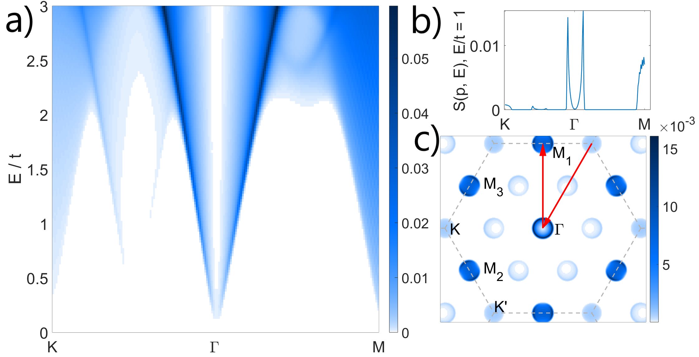
Figure 3: (a) The INS spectrum along the high-symmetry path with the same parameters in Fig. 2. In the low-energy regime of the INS spectrum, there are two strong signals at ${\bf\Gamma}$ and $\mathbf{M}$, and lighter ones at $\mathbf{K}$ and $\mathbf{K}/2$. (b) The constant energy slice of (a) at ${E/t=1}$ and is marked by the red arrow in (a). (c) The momentum dependence of ${\mathcal{S}}^{-+}(\mathbf{p},E)$ at ${E/t=1}$.

INS simulations.—To connect our results with experiments, we further calculate the spinon continuum via the transverse dynamic spin structure factor, that is proportional to the inelastic neutron spectrum differential cross-section, as

$${\mathcal{S}}^{-+}(\mathbf{p},E) =\frac{1}{N}\sum_{i,j}e^{i\mathbf{p}\cdot(\mathbf{r}_{i}-\mathbf{r}_{j})}\int e^{iEt}\langle S_{i}^{-}(t)\cdot S_{j}^{+}(0)\rangle\differential t$$ (5)

$$=\sum_{n}\delta(E-[E_{n}(\mathbf{p})-E_{0}])\left|\matrixelement{n}{S_{\mathbf{p}}^{+}}{\Omega}\right|^{2},$$

where $\ket{\Omega}$ ($\ket{n}$) and $E_{0}$ ($E_{n}$) refer to the ground (excited) state and its energy, respectively. At the mean-field level, ${\ket{\Omega}}$ is to simply fill the spinon bands below the Fermi energy, and ${S_{\bf p}^{+}=\sum_{\bf k}f_{{\bf k}-{\bf p}\uparrow}^{\dagger}f_{{\bf k}\downarrow}}$ excites one spinon particle-hole pair across the Fermi level. The summation over $n$ includes all such excited spin-1 pairs. Since the neutron scattering events involve pairs of spinons, the energy and momentum transfer of one neutron are conserved by the total energy and total momentum of two spinons. This leads to a continuous spectrum in the INS measurements, which is a strong evidence of the fractionalized excitations Shen et al. (2016); Han et al. (2012); Paddison et al. (2017) that differ from the magnon excitation with integer spins. In Fig. 3, we show the continuum along the high symmetry path. Moreover, there are other two features that arise here. First, the expected signals appear at $\mathbf{M}$ in addition to ${\bf K}$ at low energies, which agrees with the experimental results. Second, the model predicts signals at the middle point from ${\bf\Gamma}$ and ${\bf K}$. Fig. 3 shows the INS signals in the whole Brillouin zone with a fixed energy slice, including the ones around $\{\mathbf{\Gamma},\mathbf{M}_{1,2,3}\}$ and $\{\mathbf{K},\mathbf{K}^{\prime},\mathbf{K}/2,\mathbf{K}^{\prime}/2\}$.

The position of these signals is a direct consequence of the coexistence of the DSL and the supersolid order. At low energies, the spinon particle-hole pairs can be created only across the Fermi energy among those gapped Dirac cones. Therefore, the allowed momentum transfer $\mathbf{p}$’s in Eq. (5) are about the separation of Dirac cones. As shown in Fig. 3, the distribution of the Dirac cones indeed matches the pattern of the INS signal in the momentum space. The spectral continuum at $\{\mathbf{K},\mathbf{K}^{\prime},\mathbf{K}/2,\mathbf{K}^{\prime}/2\}$ is then a consequence due to the combination of the Dirac spinons and the supersolid order that has an ordering wavevector at ${\mathbf{K}},\mathbf{K}^{\prime}$. Since our theory is based on the free spinons and the Hilbert space constraint is not imposed on each site, the intra-Dirac-cone processes that contribute to the $\Gamma$ point would in principle be suppressed. This is the caveat of the free spinon theory.

Although we have obtained the continuous excitation from spinons, the fluctuation of the order parameters can still be important, and these are spin-wave excitations as magnons. These magnons can also contribute to the INS spectrum, but not usually in terms of continuous excitation. The magnons contribute to the INS spectrum as a well-defined quasiparticle-like dispersion. We calculate the spin-wave dispersion with the linear spin wave theory, and the results are depicted in Fig. 4. The gapless spectrum is due to the breaking of the U(1) symmetry. The spectrum at $\mathbf{K}$ is understood by the supersolid order with a wavevector $\mathbf{K}$, and there is a visible gap at M point. In reality, the magnetic order is strongly renormalized by the quantum correction Sheng et al. (2022), and the bandwidth of the spin-wave excitation should be suppressed compared to the linear spin-wave calculation. Taking together with the spinon continuum, the actual INS signal should be a combination of both spinon continuum and the magnonic excitations Bose et al. (2023); Lannert and Fisher (2003).

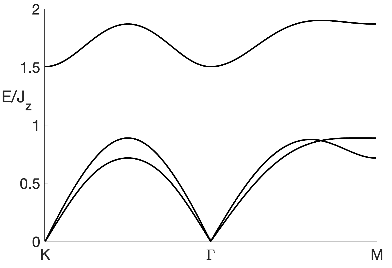
Figure 4: The spin-wave excitation from linear spin-wave theory for the supersolid state. For the Y-shape configuration, the tilting angle $\theta$ from $\hat{z}$ on the red and green sublattices (see Fig. 1) is determined by minimizing the classical exchange energy with ${\cos{\theta}=J_{z}/(J_{z}+J_{\perp})}$ and ${J_{z}=1.73J_{\perp}}$. Although this classical state is a ferrimagnet with a finite magnetization and differs slightly from the quantum supersolid, the spin-wave excitation should be a reasonable qualitative approximation of the spin-wave part of the excitations for the quantum supersolid.

Discussion.—There are two major questions that are addressed in this work. One is whether the continuous excitation in Na₂BaCo(PO₄)₂ arises from the spinon pairs. The other question is whether Na₂BaCo(PO₄)₂ has anything to do with the DSL. We provide a candidate answer to both questions by proposing a precursory DSL that combines the DSL and the supersolidity. At the mean-field level we obtained two-spinon continuum and found concentrated signals at $\{\mathbf{M},\mathbf{K},\mathbf{K}/2\}$ points. These results provide a possible candidate explanation for the bizarre INS results in Na₂BaCo(PO₄)₂. For the first question, phenomenologically two-magnon excitations could also contribute to the INS continuum Lovesey (1984). This magnon continuum, however, usually occurs at higher energies instead of the low energy, and its spectral intensity is usually weak. As for other candidate states, one natural candidate seems to be a $\mathbb{Z}_{2}$ spin liquid with condensed bosonic spinons that generate the supersolid order. We find it difficult to reconcile the magnetic structure and the position of the continuous excitations of the $\mathbb{Z}_{2}$ spin liquids that were classified with Schwinger bosons Wang and Vishwanath (2006). Phenomenologically, however, it is possible that, if one directly introduces the supersolid on top of the $\pi$-flux $\mathbb{Z}_{2}$ spin liquid in Ref. Wang and Vishwanath, 2006, one may establish a qualitatively consistent result with the experiment. We do not rule out this possibility here. Since the model for Na₂BaCo(PO₄)₂ is the easy-axis XXZ model, we expect more advanced numerical techniques to be used for the spin dynamics.

Our free-spinon mean-field theory would certainly be renormalized once the correlation (or Hilbert space constraint) is considered. This can be achieved by renormalized mean-field theory or by Gutzwillier projection Edegger et al. (2007). Except the modulation and suppression of the spectral intensities, the qualitative results for the spinon continuum should persist. With the supersolid, the precursory DSL develops a small gap, and this can potentially cause the confinement of the U(1) gauge theory. Since the U(1) DSL is regarded as the mother state for 2D magnets Song et al. (2019), one could imagine a weak spinon pairing that further stabilizes fractionalization Lu (2016). Such a state could be equivalent to a $\pi$-flux $\mathbb{Z}_{2}$ spin liquid from the Schwinger boson classification Wang and Vishwanath (2006). Nevertheless, as long as the fractionalization is present below the confinement length, one would expect continuous excitations. Moreover, thermal fluctuation suppresses the supersolid above 0.15K, and our theory expects the system to behave like a gapless DSL. In fact, a finite thermal conductivity $\kappa/T$ was observed at low temperatures above 0.15K Li et al. (2020) and is consistent with the expectation from DSL Durst and Lee (2000).

Beyond Na₂BaCo(PO₄)₂, Ref. Song et al., 2019 suggested to search for the precursory DSL among 2D frustrated lattices. One related such system that behaves like a DSL is the spin liquid candidate PrZnAl₁₁O₁₉ where the Pr ions form a triangular lattice with spin-1/2 local moments Ashtar et al. (2019); Bu et al. (2022). Moreover, even bipartite lattices with frustrated interactions can still be promising candidates, as recently proposed Bose et al. (2023); Guang et al. (2022). On more theoretical side, the fermionized vortex theory was used to describe the DSL on the triangular lattice Alicea et al. (2005) and may encounter some issue with imposing time reversal symmetry. Since time reversal is broken by the supersolid, it might be interesting to revisit the fermionized vortex theory to explore the mass generation and supersolid in the DSL.

Acknowledgments.—We particularly thank Liusuo Wu for sharing his data prior to the submission and Cenke Xu for discussion. This work is supported by NSFC with Grant No. 92065203, MOST of China with Grants No. 2021YFA1400300, and by the Research Grants Council of Hong Kong with Collaborative Research Fund C7012-21GF.

Appendix A Mean-field theory

We choose the lattice vectors as ${\mathbf{a}_{1}=(a,0)}$ and $\mathbf{a}_{2}=(a/2,\sqrt{3}a/2)$ as shown in Fig. 1 of the main text. Then, the basis vectors for the reciprocal lattice are $\mathbf{b}_{1}=({2\pi}/{a},-{2\pi}/{\sqrt{3}a})$ and ${\mathbf{b}_{2}=(0,{4\pi}/{\sqrt{3}a})}$. The high-symmetry momentum points are then defined as $\mathbf{M}=\mathbf{b}_{2}/2$, $\mathbf{K}=2\mathbf{b}_{1}/3+\mathbf{b}_{2}/3$. We will stick to this convention in the appendix.

The physical spin model is a spin-1/2 XXZ model on the triangular lattice

$$H_{\text{XXZ}}=\sum_{\langle ij\rangle}J_{\perp}(S_{i}^{x}S_{j}^{x}+S_{i}^{y}S_{j}^{y})+J_{z}S_{i}^{z}S_{j}^{z},$$ (6)

where $J_{\perp}$ and $J_{z}$ are the original spin exchange couplings. To capture both the supersolid order and the continuous excitations of this XXZ model, we implement a mean-field approach that combines the conventional Weiss type of mean-field theory for the magnetic order and the parton mean-field theory to take care of the exotic excitations. In the following, we provide a more detailed description of the mean-field theory in the main text.

A.1 Weiss mean-field channel

For the Weiss mean-field channel where $\langle S_{i}^{\mu}\rangle\neq 0$, we use a mean-field ansatz that is implied by the existing experiments and numerical studies,

$$\left\{\begin{array}[]{lll}\langle S_{i}^{x}\rangle=\frac{2\langle S_{2}^{x}\rangle\cos\phi}{\sqrt{3}}\sin{(\mathbf{K}\cdot\mathbf{r}_{i})},\vspace{2mm}\\ \langle S_{i}^{y}\rangle=\frac{2\langle S_{2}^{x}\rangle\sin\phi}{\sqrt{3}}\sin{(\mathbf{K}\cdot\mathbf{r}_{i})},\vspace{2mm}\\ \langle S_{i}^{z}\rangle=\frac{\langle S_{0}^{z}\rangle+2\langle S_{2}^{z}\rangle}{3}+2\frac{\langle S_{0}^{z}\rangle-\langle S_{2}^{z}\rangle}{3}\cos{(\mathbf{K}\cdot\mathbf{r}_{i})},\end{array}\right.$$ (10)

so that a three-sublattice Y-shape supersolid antiferromagnetic ordering is produced as

$$\left\{\begin{array}[]{lll}\mathbf{S}_{(0,0)}=(0,0,\langle S_{0}^{z}\rangle),\vspace{2mm}\\ \mathbf{S}_{\mathbf{a}_{1}}=(-\langle S_{2}^{x}\rangle\cos\phi,-\langle S_{2}^{x}\rangle\sin\phi,\langle S_{2}^{z}\rangle),\vspace{2mm}\\ \mathbf{S}_{\mathbf{a}_{2}}=(\langle S_{2}^{x}\rangle\cos\phi,\langle S_{2}^{x}\rangle\sin\phi,\langle S_{2}^{z}\rangle),\end{array}\right.$$ (14)

while $\langle\mathbf{S}_{0}\rangle$ and $\langle\mathbf{S}_{2}\rangle$ refer to the spin orders on the corresponding sublattices and can be determined self-consistently from the mean-field theory. Moreover, $\langle S^{z}_{0}\rangle=-2\langle S^{z}_{1}\rangle$. For the convenience, we set $\phi=0$.

We express the spin operator using the Abrikosov spinon representations ${S_{i}^{\mu}=\frac{1}{2}f^{\dagger}_{i\alpha}\sigma^{\mu}_{\alpha\beta}f_{i\beta}}$ with the constraint ${\sum_{\alpha}f_{i\alpha}^{\dagger}f_{i\alpha}=1}$. Then, the supersolid’s contribution to the mean-field Hamiltonian in the main text can be written as

$$H_{\text{SS}} = -\tilde{J}_{\perp}\sum_{j,\bm{\delta}_{i}}\left[\frac{\langle S_{2}^{x}\rangle}{\sqrt{3}}\sin{({\bf K}\cdot\mathbf{r}_{i})}\right](e^{-i\phi}f_{j\uparrow}^{\dagger}f_{j\downarrow}+h.c.)$$

$$+ \tilde{J}_{z}\sum_{j,\bm{\delta}_{i}}\left[\frac{\langle S_{0}^{z}\rangle+2\langle S_{2}^{z}\rangle}{6}+\frac{\langle S_{0}^{z}\rangle-\langle S_{2}^{z}\rangle}{3}\cos{(\mathbf{K}\cdot\mathbf{r}_{i})}\right]$$

$$\times (f_{j\uparrow}^{\dagger}f_{j\uparrow}-f_{j\downarrow}^{\dagger}f_{j\downarrow}),$$

where ${\mathbf{r}_{i}=\mathbf{r}_{j}+\bm{\delta}_{i}}$ with $\bm{\delta}_{i}=\{\pm\mathbf{a}_{1},\pm\mathbf{a}_{2},\pm{\mathbf{a}_{3}}\}$ with ${\mathbf{a}_{3}}={\mathbf{a}_{2}-\mathbf{a}_{1}}$ denoting the six nearest neighbours. Following the treatment of the main text, we have introduced the $\tilde{J}_{\perp}$ and $\tilde{J}_{z}$ couplings for the supersolid part of the mean-field theory. Moreover, we adopted the mean-field decoupling with,

$$\sum_{\langle ij\rangle}S_{i}^{\alpha}S_{j}^{\alpha}\rightarrow\sum_{\langle ij\rangle}\langle S_{i}^{\alpha}\rangle S_{j}^{\alpha}+S_{i}^{\alpha}\langle S_{j}^{\alpha}\rangle-\langle S_{i}^{\alpha}\rangle\langle S_{j}^{\alpha}\rangle.$$ (16)

With the Fourier transform ${f_{i\sigma}=1/\sqrt{N}\sum_{\mathbf{k}}e^{i\mathbf{k}\cdot\mathbf{r}_{i}}f_{\mathbf{k}\sigma}}$, where $N$ is the system size and the sum is over the lattice Brillouin zone (BZ),

$$H_{\text{SS}} = \frac{\sqrt{3}\tilde{J}_{\perp}\langle S_{2}^{x}\rangle}{2i}\sum_{\mathbf{k}\in\text{BZ}}\left[\left(f_{\mathbf{k+K},\uparrow}^{\dagger}f_{\mathbf{k}\downarrow}-f_{\mathbf{k-K},\uparrow}^{\dagger}f_{\mathbf{k}\downarrow}\right)+\left(f_{\mathbf{k+K},\downarrow}^{\dagger}f_{\mathbf{k}\uparrow}-f_{\mathbf{k-K},\downarrow}^{\dagger}f_{\mathbf{k}\uparrow}\right)\right]$$ (17)

$$+\tilde{J}_{z}\sum_{\mathbf{k}\in\text{BZ}}\Big{[}(\langle S_{0}^{z}\rangle+2\langle S_{2}^{z}\rangle)(f_{\mathbf{k}\uparrow}^{\dagger}f_{\mathbf{k}\uparrow}-f_{\mathbf{k}\downarrow}^{\dagger}f_{\mathbf{k}\downarrow})+\frac{\langle S_{2}^{z}\rangle-\langle S_{0}^{z}\rangle}{2}(f_{\mathbf{k+K},\uparrow}^{\dagger}f_{\mathbf{k}\uparrow}+f_{\mathbf{k-K},\uparrow}^{\dagger}f_{\mathbf{k}\uparrow}$$

$$\quad\quad\quad\quad-f_{\mathbf{k+K},\downarrow}^{\dagger}f_{\mathbf{k}\downarrow}-f_{\mathbf{k-K},\downarrow}^{\dagger}f_{\mathbf{k}\downarrow})\Big{]}.$$

Here, we used $\sum_{\bm{\delta}_{i}}e^{i\mathbf{K}\cdot\bm{\delta}_{i}}=-3$.

A.2 Spinon hopping channel

For the spinon hopping channel ($\langle f^{\dagger}_{i}f_{j}\rangle\neq 0$), as the neutron scattering data indicate the presence of a percursory Dirac spin liquid (DSL), we consider the ansatz allowed by symmetries: a U(1) DSL with only a real nearest neighbor hopping [See Fig. 5].

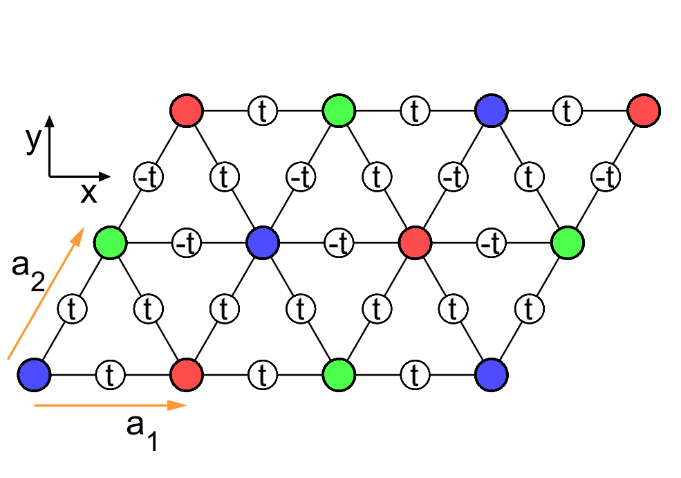
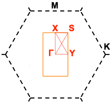
Figure 5: The upper figure is the triangular lattice formed by the Co²⁺ ions with the basis vectors ${\mathbf{a}_{1}=a(1,0)}$ and $\mathbf{a}_{2}=a(1/2,\sqrt{3}/2)$. The hopping parameters $t_{ij}$ of the spinons are indicated within the bond with a gauge choice supporting a $\pi$-flux background. In the lower figure, the black dashed lines show the lattice Brillouin zone and the orange solid lines show the magnetic Brillouin zone. The corresponding high symmetry points are also denoted.

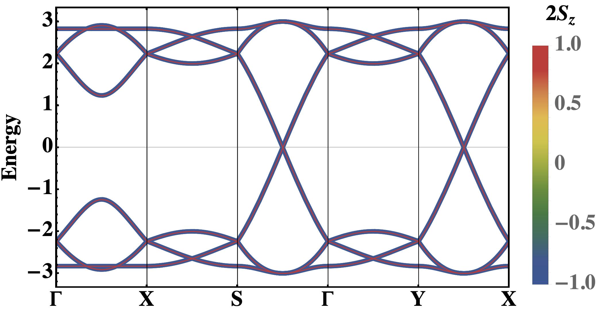
Figure 6: The band dispersions for $\tilde{J}_{z}=0$ and $\tilde{J}_{\perp}=0$. The energy is in the unit of $t$. The up-spin spinon bands in red is degenerate with the down-spin spinon bands in blue. The Dirac cones are explicitly shown.

With this ansatz, the spinon hopping part of the mean-field theory can be expressed as

$$\begin{split}H_{t}&=t\sum_{i\sigma}\left[\cos\left({\mathbf{M}\cdot\mathbf{r}_{i}}\right)\left(f_{i\sigma}^{\dagger}f_{i+\mathbf{a}_{1},\sigma}+f_{i\sigma}^{\dagger}f_{i+\mathbf{a}_{2},\sigma}\right)+f_{i\sigma}^{\dagger}f_{i+\mathbf{a}_{3},\sigma}+h.c.\right]-\mu\sum_{i\sigma}f_{i\sigma}^{\dagger}f_{i\sigma}\\ &=\sum_{\mathbf{k}\in\text{BZ}}\sum_{\sigma}(2t\cos\left({\mathbf{k}\cdot\mathbf{a}_{3}}\right)-\mu)f_{\mathbf{k}\sigma}^{\dagger}f_{\mathbf{k}\sigma}\\ &+\sum_{\mathbf{k}\in\text{BZ}}\sum_{\sigma}\left[t\frac{e^{i\mathbf{k}\cdot\mathbf{a}_{1}}+e^{i\mathbf{k}\cdot\mathbf{a}_{2}}}{2}\left(f_{\mathbf{k+M},\sigma}^{\dagger}f_{\mathbf{k}\sigma}+f_{\mathbf{k-M},\sigma}^{\dagger}f_{\mathbf{k}\sigma}\right)+t\frac{e^{-i\mathbf{k}\cdot\mathbf{a}_{1}}+e^{-i\mathbf{k}\cdot\mathbf{a}_{2}}}{2}\left(f_{\mathbf{k}\sigma}^{\dagger}f_{\mathbf{k-M},\sigma}+f_{\mathbf{k}\sigma}^{\dagger}f_{\mathbf{k+M},\sigma}\right)\right]\\ &=\sum_{\mathbf{k}\in\text{BZ},\sigma}(2tA_{\mathbf{k}}-\mu)f_{\mathbf{k}\sigma}^{\dagger}f_{\mathbf{k}\sigma}+tB_{\mathbf{k}}f_{\mathbf{k}\sigma}^{\dagger}f_{\mathbf{k+M},\sigma}+tB^{*}_{\mathbf{k}}f_{\mathbf{k+M},\sigma}^{\dagger}f_{\mathbf{k}\sigma},\end{split}$$ (18)

where ${A_{\mathbf{k}}=\cos\left({\mathbf{k}\cdot\mathbf{a}_{3}}\right)},\ {B_{\mathbf{k}}=\cos{(\mathbf{k}\cdot\mathbf{a}_{1})}-i\sin{(\mathbf{k}\cdot\mathbf{a}_{2})}}$, and we have used the fact that $2\mathbf{M}=\mathbf{b}_{2}$.

Since the U(1) DSL ansatz gives rise to a $\pi$-flux background and doubling of the spinon unit cell, along with the presence of the supersolid ordering, the size of the magnetic Brillouin zone (MBZ) is 1/6 as large as the size of the lattice Brillouin zone in Fig. 5. In order to obtain the dispersion of the spinon excitations, we need to fold the lattice Brillouin zone (BZ) into MBZ and formally convert the sum over $\mathbf{k}\in\text{BZ}$ in Eqs. (17) and (18) into the summation over $\mathbf{k}^{\prime}\in\text{MBZ}$ as

$$\sum_{\mathbf{k}\in\text{BZ}}=\sum_{\mathbf{k}^{\prime}}+\!\!\sum_{\mathbf{k^{\prime}+M}}+\!\!\sum_{\mathbf{k^{\prime}+K}}+\!\!\sum_{\mathbf{k^{\prime}+K+M}}+\!\!\sum_{\mathbf{k^{\prime}-K}}+\!\!\sum_{\mathbf{k^{\prime}-K+M}},$$ (19)

where ${\mathbf{k}^{\prime}\in\text{MBZ}}$ is implicitly assumed on the right hand side. Using the fact that ${3\mathbf{K}=\mathbf{b}_{1}-\mathbf{b}_{2}}$ and ${2\mathbf{M}=\mathbf{b}_{2}}$, we can express the whole mean-field Hamiltonian in MBZ as

$$H_{\text{MF}}=\sum_{\mathbf{k}\in\text{MBZ}}X_{\mathbf{k}}^{\dagger}H_{\mathbf{k}}X_{\mathbf{k}}$$ (20)

with $X_{\mathbf{k}}=$$\left(f_{\mathbf{k}\uparrow},\,f_{\mathbf{k}\downarrow},\,f_{\mathbf{k+M}\uparrow},\,f_{\mathbf{k+M}\downarrow},\,f_{\mathbf{k+K}\uparrow},\,f_{\mathbf{k+K}\downarrow},\,f_{\mathbf{k+K+M}\uparrow},\right.$ $\left.\,f_{\mathbf{k+K+M}\downarrow},\,f_{\mathbf{k-K}\uparrow},\,f_{\mathbf{k-K}\downarrow},\,f_{\mathbf{k-K+M}\uparrow},\,f_{\mathbf{k-K+M}\downarrow}\right)^{T}$, and

$$H_{\mathbf{k}}=H_{t,\mathbf{k}}+H_{SS,\mathbf{k}} =\begin{bmatrix}H_{0}(\mathbf{k})&&\\ &H_{0}(\mathbf{k+K})&\\ &&H_{0}(\mathbf{k-K})\end{bmatrix}$$

$$+\begin{bmatrix}V&H_{1}&H_{1}^{\dagger}\\ H_{1}^{\dagger}&V&H_{1}\\ H_{1}&H_{1}^{\dagger}&V\end{bmatrix},$$ (21)

where the blank entries refer to 0, and

$$H_{0}(\mathbf{k}) =2t\begin{bmatrix}A_{\mathbf{k}}&B_{\mathbf{k}}\vspace{2mm}\\ B^{*}_{\mathbf{k}}&-A_{\mathbf{k}}\end{bmatrix}\otimes{\mathcal{I}}_{2}-\mu\,\mathcal{I}_{4},$$ (22)

$$V =\tilde{J}_{z}\big{[}\langle S_{0}^{z}\rangle+2\langle S_{2}^{z}\rangle\big{]}{\mathcal{I}}_{2}\otimes\sigma_{z},$$ (23)

$$H_{1} =\tilde{J}_{z}\frac{\langle S_{2}^{z}\rangle-\langle S_{0}^{z}\rangle}{2}{\mathcal{I}}_{2}\otimes\sigma_{z}-\tilde{J}_{\perp}\frac{\sqrt{3}\langle S_{2}^{x}\rangle}{2i}{\mathcal{I}}_{2}\otimes\sigma_{x}.$$ (24)

Here ${\mathcal{I}}_{2}$ and ${\mathcal{I}}_{4}$ are $2\times 2$ and $4\times 4$ identity matrix, respectively. By diagonalizing Eq. (20), we obtain 12 spinon bands in the MBZ as shown in the main text and in the following section.

Appendix B Effects of the quantum supersolid order

In the absence of the spin order $\langle S_{0}^{z}\rangle=\langle S_{2}^{z}\rangle=\langle S_{2}^{x}\rangle=0$, the mean-field Hamiltonian in the previous section gives rise to gapless Dirac cones at the spinon Fermi level. There are two Dirac cones for each spin in the MBZ as shown in Fig. 6. The spinon bands are colored by ${\langle\hat{S}_{z}(\mathbf{k})\rangle=\langle\psi_{n,\mathbf{k}}|\hat{S}_{z}|\psi_{n,\mathbf{k}}\rangle}$, where $|\psi_{n,\mathbf{k}}\rangle$ is the wavefunction for the $n$-th spinon band, $\hat{S}_{z}$ is the $z$-component of the spin operator and can be expressed as $\mathcal{I}_{6\times 6}\otimes\frac{1}{2}\sigma_{z}$ in the basis of $X_{\mathbf{k}}$.

To explore the properties of the Dirac spinons, in a usual treatment, one analyzes the symmetry properties of various mass gap terms for the Dirac cones and establishes the connection between the mass gaps with the physical spin observables. Here we have already known the magnetic orders of the system. We can then directly study the evolution of the spinon spectrum in the presence of the spin supersolid. With the supersolid order in the main text, we have ${\langle S_{0}^{z}\rangle+2\langle S_{2}^{z}\rangle=0}$ and ${V=0}$ in Eq. (21).

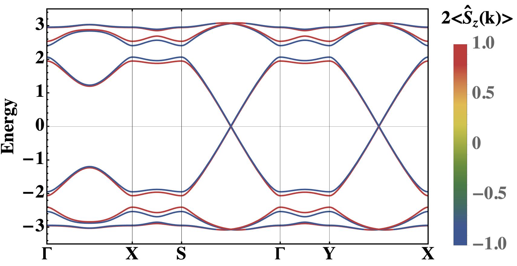
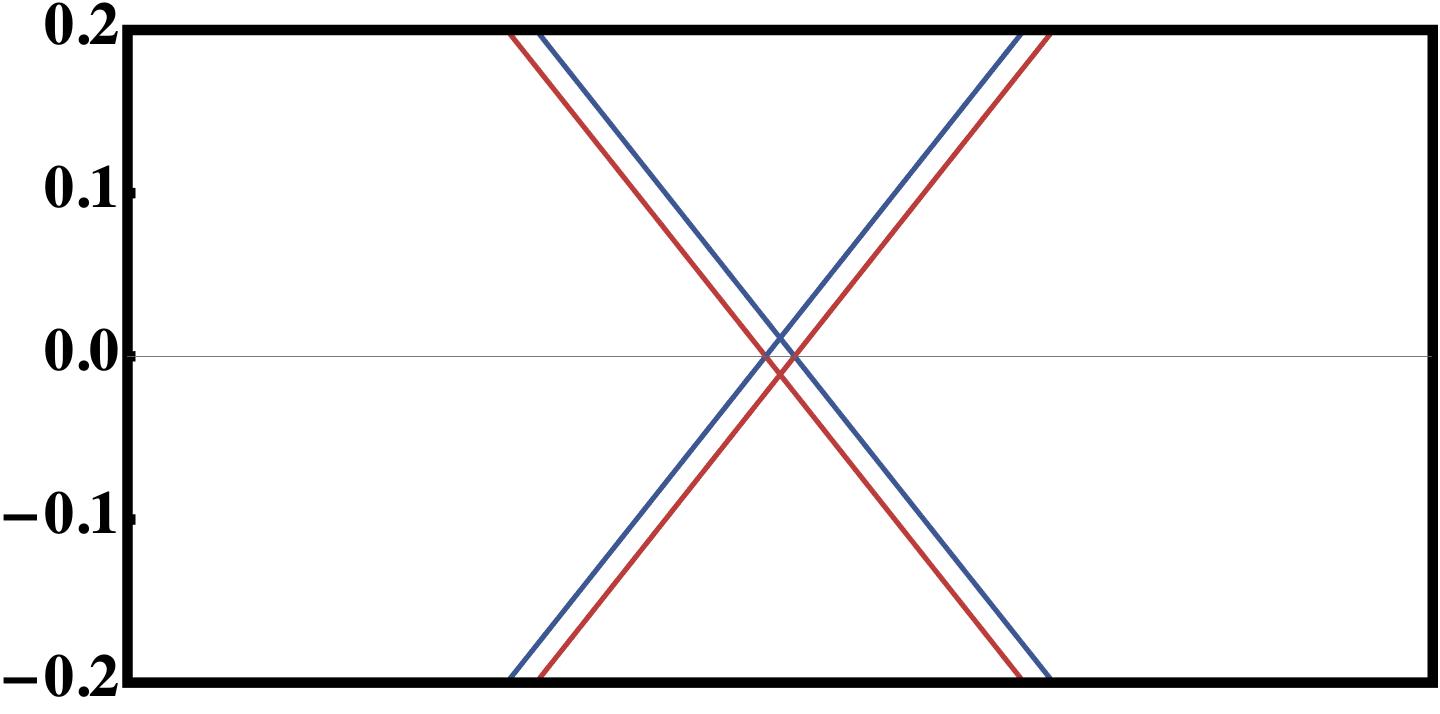
Figure 7: The upper figure is the spinon band dispersions for ${\tilde{J}_{z}|\langle S_{0}^{z}\rangle|=0.5t}$ and ${\tilde{J}_{\perp}\langle S_{2}^{x}\rangle=0}$. Energy is in the unit of $t$. The red (blue) Dirac cones formed by up-spin (down-spin) bands do not open the gap. The lower figure is the spinon dispersion near the Fermi level where the gapless feature persists.

The supersolid order carries both the Ising antiferromagnetic order in $z$ and the in-plane $xy$ antiferromagnetic order, where the former is often referred as the density wave order and the latter is referred as the superfluid order in the hardcore boson language for the spins. Due to the presence of two such orders, it is a bit illuminating to separately study the impact on the gapless Dirac cones one by one. We begin with the Ising order by setting $\langle S^{x}\rangle=0$. As shown in Fig. 7, the degeneracy in Fig. 6 is lifted by $H_{1}$ with $\tilde{J}_{z}(\langle S_{0}^{z}\rangle-\langle S_{2}^{z}\rangle)\neq 0$. Since the spin-$z$ is still a good quantum number to label the spinon bands, the two cones from different spin sectors do not mix with each other, and the Dirac cones at the Fermi level remain gapless except the breaking of the original four-fold degeneracy (see Fig. 7). In the presence of both Ising and in-plane orders for the actual supersolid, the $\tilde{J}_{\perp}\langle S_{2}^{x}\rangle$ term in $H_{1}$ does not commute with $\hat{S}_{z}$, and this in-plane order immediately creates the gap for the Dirac spinons at the Fermi level by the spin mixing as shown in Fig. 8.

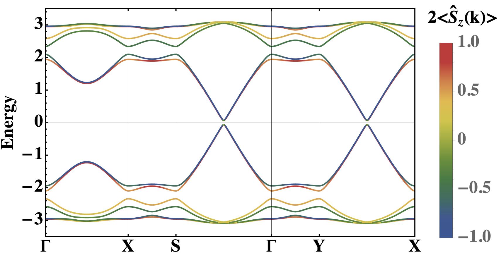
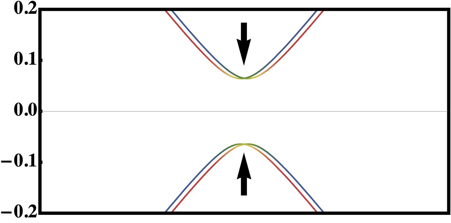
Figure 8: The upper figure is the spinon band dispersion with the same parameters in the main text that $(\langle S_{0}^{z}\rangle,\ \langle S_{2}^{z}\rangle,\ \langle S_{2}^{x}\rangle)=(-0.108,\ 0.054,\ 0.0393)$ and $(\tilde{J}_{z},\ \tilde{J}_{\perp})=(4.394,4.102)t$. Energy is in the unit of $t$. The lower figure is the spinon dispersion near the Fermi level where the yellow and green bands clearly show that the gaps resulting from the spin-mixing.

Appendix C Vanishing Chern number of filled spinon bands

With the quantum supersolid order, the Dirac cones at the Fermi level acquire the mass gap, and the 6 filled spinon bands under the Fermi level are well separated from the upper 6 spinon bands. As the time reversal symmetry is already broken by the supersolid order, it is then natural to know whether the filled spinon bands support a nontrivial Chern number. When one goes beyond the mean-field theory, the gapped spinon bands with a nontrivial Chern number could induce a Chern-Simon term in the U(1) gauge theory that is very much like the one in chiral spin liquids.

Since all these bands are now overlapping in energy, one the needs to invoke the non-Abelian Berry connection to define the Chern number of the filled bands. The Chern number of the total 6 filled spinon bands are well defined by an integral over the continuum magnetic Brillouin zone (MBZ) as

$$C_{-}=\frac{1}{2\pi i}\int_{\text{MBZ}}\text{Tr}\,\big{[}\,d_{\mathbf{k}}\mathcal{A}^{-}_{\mathbf{k}}\big{]},$$ (25)

where the non-Abelian Berry connection Wilczek and Zee (1984)

$$\mathcal{A}^{-}_{\mathbf{k}}={\psi^{-}_{\mathbf{k}}}^{\dagger}{d}_{\mathbf{k}}\psi^{-}_{\mathbf{k}}$$ (26)

is a $6\times 6$ matrix-valued one-form in the momentum $\mathbf{k}$-space associated with the wavefunctions for the filled spinon bands $\psi^{-}_{\mathbf{k}}=(|\psi^{-}_{1\mathbf{k}}\rangle,...,|\psi^{-}_{6\mathbf{k}}\rangle)$.

Numerically we evaluate this Chern number using the Fukui method Fukui et al. (2005) in the $M\times M$-grid discrete momentum space $k_{l}=(\frac{2\pi}{3Ma}j_{x},\frac{\pi}{Ma\sqrt{3}}j_{y})$ ($j_{\mu}=0,...,.M-1$ for $\mu=x,y$) as

$$\tilde{C}_{-}=\frac{1}{2\pi i}\sum_{l}\tilde{F}_{xy}(k_{l}),$$ (27)

where the lattice field strength

$$\tilde{F}_{xy}(k_{l})=\ln[U_{x}(k_{l})U_{y}(k_{l}+\hat{x})U_{x}(k_{l}+\hat{y})^{-1}U_{y}(k_{l})^{-1}]$$ (28)

with $\hat{x}=(\frac{2\pi}{3Ma},0)$ and $\hat{y}=(0,\frac{\pi}{Ma\sqrt{3}})$, and the link variable

$$U_{\mu}(k_{l})=\left|\text{det}\left[{\psi^{-}}^{\dagger}_{k_{l}}{\psi^{-}}_{k_{l}+\hat{\mu}}\right]\right|^{-1}\text{det}\left[{\psi^{-}}^{\dagger}_{k_{l}}{\psi^{-}}_{k_{l}+\hat{\mu}}\right].$$ (29)

With the periodic boundary condition, the MBZ is a closed two-dimensional torus $T^{2}$, guaranteeing the Chern number an integer. Then, with sufficiently fine grids, the Chern number on the discretized space $\tilde{C}_{-}$ equals to $C_{-}$, and we find ${\tilde{C}_{-}=0}$ up to a grid choice ${M=300}$. Thus, we conclude that the gap opening from the precursory DSL with the supersolid order is not topological and there is no Chern-Simons term.

Appendix D More discussion about quantum spin supersolid and Dirac fermions

Since Na₂BaCo(PO₄)₂ realizes the quantum spin supersolid at low temperatures and we have further proposed a precursory Dirac spin liquid for it, it is worthwhile to raise some further discussion about the proximate states out of the quantum spin supersolid and some of the related properties. This may provide some further insights for the interested readers. The material Na₂BaCo(PO₄)₂ is located in the fully frustrated regime of the XXZ model on the triangular lattice and thus has a sign problem for quantum Monte Carlo simulation. Most of the early analysis of the triangular lattice XXZ model were devoted to the less frustrated regime of the XXZ model, i.e. ${J_{\perp}<0}$ where the quantum supersolid is well present before the knowledge on the fully frustrated side due to the absence of the sign problem Melko et al. (2005); Wessel and Troyer (2005). The intimate relation between the fully frustrated regime with ${J_{\perp}>0}$ and the less frustrated regime with ${J_{\perp}<0}$ was partially addressed in Ref. Wang et al., 2009. It was shown that Wang et al. (2009), in the perturbative regime ${J_{\perp}\ll J_{z}}$, one can perform a unitary transformation to connect both regimes. This establishes the presence of the supersolid in the fully frustrated regime and argued to extend to the Heisenberg point based on the continuity argument. This unitary transformation that connects the fully frustrated and less frustrated regime is analogous to the one that was used in the pyrochlore spin ice context Hermele et al. (2004).

On the less frustrated side with ${J_{\perp}<0}$, due to the underlying U(1) symmetry of the XXZ model, a boson-vortex duality was adopted to explore the proximate states and phase transitions by viewing the spins as hardcore bosons Burkov and Balents (2005). It was predicted from an emergent SU(2) symmetry that, the quantum supersolid is proximate to deconfined quantum criticality of the NCCP¹ universality class. Remarkably, this is identical to the Néel-VBS transition. From the recent duality argument, this criticality is dual to the ${N_{f}=2}$ fermionic quantum electrodynamics with Dirac fermions Wang et al. (2017). Although this is on the less frustrated side and may not be directly related to Na₂BaCo(PO₄)₂, it provides some insights about the connection between the quantum supersolid and the Dirac fermions, and may be useful for the full understanding of the nearby phases of the quantum supersolids in both regimes.

References

- Kramers and Wannier (1941) H. A. Kramers and G. H. Wannier, Phys. Rev. 60, 252 (1941).
- Fisher and Lee (1989) M. P. A. Fisher and D. H. Lee, Phys. Rev. B 39, 2756 (1989).
- Fisher (2004) M. P. A. Fisher, “Duality in low dimensional quantum field theories,” in Strong interactions in low dimensions, edited by D. Baeriswyl and L. Degiorgi (Springer Netherlands, Dordrecht, 2004) pp. 419–438.
- Balents et al. (1999) L. Balents, M. P. A. Fisher, and C. Nayak, Phys. Rev. B 60, 1654 (1999).
- Balents et al. (2005) L. Balents, L. Bartosch, A. Burkov, S. Sachdev, and K. Sengupta, Physical Review B 71, 144508 (2005).
- Karch and Tong (2016) A. Karch and D. Tong, Phys. Rev. X 6, 031043 (2016).
- Son (2015) D. T. Son, Physical Review X 5, 031027 (2015).
- Wang and Senthil (2016) C. Wang and T. Senthil, Physical Review X 6, 011034 (2016).
- Wang et al. (2017) C. Wang, A. Nahum, M. A. Metlitski, C. Xu, and T. Senthil, Phys. Rev. X 7, 031051 (2017).
- Song et al. (2019) X.-Y. Song, C. Wang, A. Vishwanath, and Y.-C. He, Nature Communications 10, 4254 (2019).
- Chen et al. (2009) G. Chen, L. Balents, and A. P. Schnyder, Phys. Rev. Lett. 102, 096406 (2009).
- Chen (2017) G. Chen, Phys. Rev. B 96, 020412 (2017).
- Li and Chen (2019) F.-Y. Li and G. Chen, Phys. Rev. B 100, 045103 (2019).
- Su et al. (2019) N. Su, F. Li, Y. Jiao, Z. Liu, J. Sun, B. Wang, Y. Sui, H. Zhou, G. Chen, and J. Cheng, Science Bulletin 64, 1222 (2019).
- Witczak-Krempa et al. (2014) W. Witczak-Krempa, G. Chen, Y. B. Kim, and L. Balents, Annual Review of Condensed Matter Physics 5, 57 (2014).
- Lee et al. (2010) S. Lee, R. K. Kaul, and L. Balents, Nature Physics 6, 702 (2010).
- Faure et al. (2018) Q. Faure, S. Takayoshi, S. Petit, V. Simonet, S. Raymond, L.-P. Regnault, M. Boehm, J. S. White, M. Månsson, C. Rüegg, P. Lejay, B. Canals, T. Lorenz, S. C. Furuya, T. Giamarchi, and B. Grenier, Nature Physics 14, 716 (2018).
- Wang et al. (2015) Z. Wang, M. Schmidt, A. K. Bera, A. T. M. N. Islam, B. Lake, A. Loidl, and J. Deisenhofer, Phys. Rev. B 91, 140404 (2015).
- Zou et al. (2021) H. Zou, Y. Cui, X. Wang, Z. Zhang, J. Yang, G. Xu, A. Okutani, M. Hagiwara, M. Matsuda, G. Wang, G. Mussardo, K. Hódsági, M. Kormos, Z. He, S. Kimura, R. Yu, W. Yu, J. Ma, and J. Wu, Phys. Rev. Lett. 127, 077201 (2021).
- Wang et al. (2018a) Z. Wang, T. Lorenz, D. I. Gorbunov, P. T. Cong, Y. Kohama, S. Niesen, O. Breunig, J. Engelmayer, A. Herman, J. Wu, K. Kindo, J. Wosnitza, S. Zherlitsyn, and A. Loidl, Phys. Rev. Lett. 120, 207205 (2018a).
- Wang et al. (2018b) Z. Wang, J. Wu, W. Yang, A. K. Bera, D. Kamenskyi, A. T. M. N. Islam, S. Xu, J. M. Law, B. Lake, C. Wu, and A. Loidl, Nature 554, 219 (2018b).
- Liu et al. (2020) H. Liu, J. c. v. Chaloupka, and G. Khaliullin, Phys. Rev. Lett. 125, 047201 (2020).
- Liu and Khaliullin (2018) H. Liu and G. Khaliullin, Phys. Rev. B 97, 014407 (2018).
- Sano et al. (2018) R. Sano, Y. Kato, and Y. Motome, Phys. Rev. B 97, 014408 (2018).
- Morris et al. (2021) C. M. Morris, N. Desai, J. Viirok, D. Hüvonen, U. Nagel, T. Rõõm, J. W. Krizan, R. J. Cava, T. M. McQueen, S. M. Koohpayeh, R. K. Kaul, and N. P. Armitage, Nature Physics 17, 832 (2021).
- Ringler et al. (2022) J. A. Ringler, A. I. Kolesnikov, and K. A. Ross, Phys. Rev. B 105, 224421 (2022).
- Sheng et al. (2022) J. Sheng, L. Wang, A. Candini, W. Jiang, L. Huang, B. Xi, J. Zhao, H. Ge, N. Zhao, Y. Fu, et al., Proceedings of the National Academy of Sciences 119, e2211193119 (2022).
- Li et al. (2020) N. Li, Q. Huang, X. Y. Yue, W. J. Chu, Q. Chen, E. S. Choi, X. Zhao, H. D. Zhou, and X. F. Sun, Nature Communications 11, 4216 (2020).
- Yamamoto et al. (2014a) D. Yamamoto, G. Marmorini, and I. Danshita, Phys. Rev. Lett. 112, 127203 (2014a).
- Wang et al. (2009) F. Wang, F. Pollmann, and A. Vishwanath, Phys. Rev. Lett. 102, 017203 (2009).
- (31) Private communication with Dr. Liusuo Wu.
- Ito et al. (2017) S. Ito, N. Kurita, H. Tanaka, S. Ohira-Kawamura, K. Nakajima, S. Itoh, K. Kuwahara, and K. Kakurai, , 235 (2017).
- Ma et al. (2016) J. Ma, Y. Kamiya, T. Hong, H. B. Cao, G. Ehlers, W. Tian, C. D. Batista, Z. L. Dun, H. D. Zhou, and M. Matsuda, Phys. Rev. Lett. 116, 087201 (2016).
- Sherman et al. (2022) N. E. Sherman, M. Dupont, and J. E. Moore, arXiv e-prints , arXiv:2209.00739 (2022), arXiv:2209.00739 [cond-mat.str-el] .
- Ferrari and Becca (2019) F. Ferrari and F. Becca, Phys. Rev. X 9, 031026 (2019).
- Iqbal et al. (2016) Y. Iqbal, W.-J. Hu, R. Thomale, D. Poilblanc, and F. Becca, Phys. Rev. B 93, 144411 (2016).
- Zhong et al. (2019) R. Zhong, S. Guo, G. Xu, Z. Xu, and R. J. Cava, Proceedings of the National Academy of Sciences 116, 14505 (2019).
- Yamamoto et al. (2014b) D. Yamamoto, G. Marmorini, and I. Danshita, Physical Review Letters 112, 127203 (2014b).
- Wessel and Troyer (2005) S. Wessel and M. Troyer, Physical review letters 95, 127205 (2005).
- Melko et al. (2005) R. Melko, A. Paramekanti, A. Burkov, A. Vishwanath, D. Sheng, and L. Balents, Physical review letters 95, 127207 (2005).
- Shen et al. (2016) Y. Shen, Y.-D. Li, H. Wo, Y. Li, S. Shen, B. Pan, Q. Wang, H. Walker, P. Steffens, M. Boehm, et al., Nature 540, 559 (2016).
- Affleck et al. (1988) I. Affleck, Z. Zou, T. Hsu, and P. W. Anderson, Phys. Rev. B 38, 745 (1988).
- Han et al. (2012) T.-H. Han, J. S. Helton, S. Chu, D. G. Nocera, J. A. Rodriguez-Rivera, C. Broholm, and Y. S. Lee, Nature 492, 406 (2012).
- Paddison et al. (2017) J. A. Paddison, M. Daum, Z. Dun, G. Ehlers, Y. Liu, M. B. Stone, H. Zhou, and M. Mourigal, Nature Physics 13, 117 (2017).
- Bose et al. (2023) A. Bose, M. Routh, S. Voleti, S. K. Saha, M. Kumar, T. Saha-Dasgupta, and A. Paramekanti, “Proximate Dirac spin liquid in the - XXZ model for honeycomb cobaltates,” (2023), arXiv:2212.13271 [cond-mat.str-el] .
- Lannert and Fisher (2003) C. Lannert and M. Fisher, International Journal of Modern Physics B 17, 2821 (2003).
- Lovesey (1984) S. Lovesey, Theory of Neutron Scattering from Condensed Matter: Nuclear scattering, International series of monographs on physics (Clarendon Press, 1984).
- Wang and Vishwanath (2006) F. Wang and A. Vishwanath, Phys. Rev. B 74, 174423 (2006).
- Edegger et al. (2007) B. Edegger, V. N. Muthukumar, and C. Gros, Advances in Physics 56, 927 (2007).
- Lu (2016) Y.-M. Lu, Phys. Rev. B 93, 165113 (2016).
- Durst and Lee (2000) A. C. Durst and P. A. Lee, Phys. Rev. B 62, 1270 (2000).
- Ashtar et al. (2019) M. Ashtar, M. A. Marwat, Y. X. Gao, Z. T. Zhang, L. Pi, S. L. Yuan, and Z. M. Tian, J. Mater. Chem. C 7, 10073 (2019).
- Bu et al. (2022) H. Bu, M. Ashtar, T. Shiroka, H. C. Walker, Z. Fu, J. Zhao, J. S. Gardner, G. Chen, Z. Tian, and H. Guo, Phys. Rev. B 106, 134428 (2022).
- Guang et al. (2022) S. K. Guang, N. Li, R. L. Luo, Q. Huang, Y. Y. Wang, X. Y. Yue, K. Xia, Q. J. Li, X. Zhao, G. Chen, H. D. Zhou, and X. F. Sun, “Thermal Transport of Fractionalized Antiferromagnetic and Field Induced States in the Kitaev Material Na2Co2TeO6,” (2022), arXiv:2211.07914 [cond-mat.str-el] .
- Alicea et al. (2005) J. Alicea, O. I. Motrunich, and M. P. A. Fisher, Phys. Rev. Lett. 95, 247203 (2005).
- Wilczek and Zee (1984) F. Wilczek and A. Zee, Phys. Rev. Lett. 52, 2111 (1984).
- Fukui et al. (2005) T. Fukui, Y. Hatsugai, and H. Suzuki, Journal of the Physical Society of Japan 74, 1674 (2005).
- Hermele et al. (2004) M. Hermele, M. P. A. Fisher, and L. Balents, Phys. Rev. B 69, 064404 (2004).
- Burkov and Balents (2005) A. A. Burkov and L. Balents, Phys. Rev. B 72, 134502 (2005).