Deep Convolutional Tables:
Deep Learning without Convolutions

Abstract

We propose a novel formulation of deep networks that do not use dot-product neurons and rely on a hierarchy of voting tables instead, denoted as Convolutional Tables (CT), to enable accelerated CPU-based inference. Convolutional layers are the most time-consuming bottleneck in contemporary deep learning techniques, severely limiting their use in Internet of Things and CPU-based devices. The proposed CT performs a fern operation at each image location: it encodes the location environment into a binary index and uses the index to retrieve the desired local output from a table. The results of multiple tables are combined to derive the final output. The computational complexity of a CT transformation is independent of the patch (filter) size and grows gracefully with the number of channels, outperforming comparable convolutional layers. It is shown to have a better capacity:compute ratio than dot-product neurons, and that deep CT networks exhibit a universal approximation property similar to neural networks. As the transformation involves computing discrete indices, we derive a soft relaxation and gradient-based approach for training the CT hierarchy. Deep CT networks have been experimentally shown to have accuracy comparable to that of CNNs of similar architectures. In the low compute regime, they enable an error:speed trade-off superior to alternative efficient CNN architectures.

I Introduction

Deep learning techniques in general, and convolutional neural networks (CNNs) in particular, have become the core computational approach in computer vision. Currently, ‘deep learning techniques’ and ‘deep neural networks’ are synonyms, despite relating to different concepts. By definition [9], deep learning is the “use of multiple layers to progressively extract higher-level features from raw input,” i.e., learning a useful feature hierarchy. Artificial neural networks, on the other hand, are graphs of dot-products/convolutions computing elements. In this work, we argue that it is possible to unravel this dualism, and that this is a worthwhile endeavor.

It is the need for accelerated and more efficient CPU-based inference that has motivated us to depart from the dot-product/convolution-based paradigm. CNNs consist of millions of ‘neurons’: computing elements applying dot products to their inputs. The resulting computational load is significant and is usually handled by GPUs and other specialized hardware. Due to these computational demands, deep learning applications are often restricted to the server-side, where powerful dedicated hardware carries the computational load. Alternatively, applications running on standard CPUs or low-computing platforms such as cellphones are limited to small, low-accuracy networks, or avoid using networks altogether. Such applications are natural user interfaces (NUIs), face recognition, mobile robotics, and Internet of Things (IoT) devices, to name a few. Low-compute platforms are not equipped with a GPU and are expected to handle the inference of simple deep learning tasks. Such devices are unable to train CNNs or run ImageNet-scale CNNs. Other devices of interest, such as most laptops and desktop computers, are unequipped with GPUs but have gigabytes of memory.

In this work, we propose a novel deep learning paradigm based on a hierarchy of deep voting tables. This allows the embedding of input signals such as images, similarly to backbone CNNs, which is shown to be preferable in low-compute and GPU-less domains. Our approach uses CPUs that are capable of efficiently accessing large memory domains (random access). For instance, for a CPU with ideally unbounded memory access, the fastest classifier is a single huge table: a series of simple binary queries is applied to the input, an index is built from the resulting bits, and an answer is retrieved from the table entry. Such an approach is impractical due to the huge size of the resulting table. A practical alternative is to replace the single table with an ensemble of smaller hierarchical tables. Rather than rely on dot products, we propose a two-step, computationally efficient alternative. First, a set of $K$ simple binary queries is applied to the input patch, thus encoding it with a binary codeword of $K$-bit. Second, the computed codeword is used as an index into a table to retrieve the corresponding output representation. The proposed transformation is called a Convolutional Table (CT). A CT layer consists of multiple CTs whose outputs are summed. Similarly to convolutional layers, CT layers are stacked to form a CT network and derive a hierarchy of features. We detail this construction in Section III.

A fern is a tree in which all split criteria at a fixed tree depth are identical, such that the leaf identity is determined by using fixed $K$ split criteria termed ’bit-functions’. The CT operation is the application of a single fern to a single input location, and the operation of a CT layer (sum of CTs), corresponds to applying a fern ensemble. In Section IV, we compare the computational complexity of the CNN and CT operations. By design, the complexity of a single CT layer is independent of the size of the patch used (‘filter size’ in a convolutional layer), and its dependence on quadratic depth terms is with significantly lower constants. This allows us to derive conditions for which a CT network can be considerably faster than a corresponding CNN.

In Section V, we derive rigorous results regarding the capacity of a single fern and the expressiveness of a two-layer CT network. Specifically, the VC dimension of a single fern with $K$ bits is shown to be $\Theta(2^{K})$. This implies that a fern has an advantage over a dot product operation: it has a significantly higher capacity-to-computing-effort ratio. Our results show that a two-layered CT network has the same universal approximation capabilities as a two-layered neural network, and that this also holds for ferns with a single bit-function per fern.

A core challenge of the proposed deep-table approach is the need for a proper training process. The challenge arises because inference requires computing discrete indices that are unnameable for gradient-based learning. Thus, we introduce in Section VI a ‘soft formulation of the calculation of the $K$ bit codeword’, as a Cartesian product of the $K$ soft bit functions. Following [23, 37], bit-functions are computed by comparing only two pixels in the region of interest. However, in their soft version, the pixel indices parameters are non-integer, and their gradient-based optimization relies on the horizontal and vertical spatial gradients of the input maps. During training, soft indices are used for table voting using a weighted combination of possible votes. We use an annealing mechanism and an incremental learning schedule to gradually turn trainable but inefficient soft voting into efficient, hard single-word voting at the inference time.

We developed a CPU-based implementation of the proposed scheme and applied it to multiple standard data-sets, consisting of up to 250K images. The results, presented in Section VII, show that CT-networks achieve an accuracy comparable to CNNs with similar structural parameters while outperforming the corresponding CNNs trained using weights and activations binarization. More importantly, we consider the speed:error and speed:error:memory trade-offs, where speed is estimated via operation count. CT networks have been shown to provide better speed:error trade-off than efficient CNN architectures such as MobileNet [35] and ShuffleNet [29] in the tested domain. The improved speed:error trade-off requires a higher memory consumption, as CT networks essentially trade speed for memory. Overall, CT networks can provide $3.1-12X$ acceleration over CNNs with memory expansions of $2.3X-10.6X$, which are applicable for laptops and IoT applications.

In summary, our contribution in this paper is two-fold: First, we present an alternative to convolution-based networks and show for the first time that useful deep learning (i.e., learning of a feature hierarchy) can be achieved by other means.  Second, from an applicable viewpoint, we suggest a framework enabling accelerated CPU inference for low-compute domains, with moderate costs of accuracy degradation and memory consumption.

II Related Work

Computationally efficient CNN schemes were extensively studied using a plethora of approaches, such as low-rank or tensor decomposition [18], weight quantization [2, 20], conditional computation  [8, 3, 1], using FFT for efficient convolution computations [32], or pruning of networks weights and filters [26, 13, 6, 40]. In the following, we focus on the methods most related to our work.

Binarization schemes aim to optimize CNNs by binarizing network weights [31, 28, 7] and internal network activations [34, 27]. Recent approaches apply weights-activations-based binarization [4], to reduce memory footprint and computational complexity by utilizing only binary operations. Methods which binarize the activations are related to the proposed scheme, as they encode each local environment into a binary vector. However, their encoding is dense, and the output is computed using a (binary) dot product. The proposed scheme also utilizes binary activations, but differs significantly, as convolution/dot product operations are not applied. In contrast, we apply binary comparisons between random samples in the activation maps.

Knowledge distillation approaches [15, 44] use a large “Teacher” CNN  to train a smaller computationally efficient “Student” CNN. We show in our experiments that this technique can be combined with our approach to improve the accuracy. Regarding network design, several architectures were suggested for low-compute platforms [35, 29, 41, 11], utilizing group convolutions [35], efficient depth-wise convolutions [35, 29], map shifts [41], dubbed Bi-Real net [28] and sparse convolutions [11]. Differentiable soft quantization was proposed by Gong et al. [12] to quantize the weights of a CNN to a given number of bits. A paper by Huang et al. [16] proposed a method for efficient quantization using a multilevel binarization technique and a linear or logarithmic quantizer to simultaneously binarize weights and quantize activations to a low bit width. The authors of the paper then compare the trade-offs of this method to low-compute versions of MobileNetV2 [35], ShuffleNet [29] and Bi-Real Net [28]. The use of trees or ferns applied using convolutions for fast predictors was thoroughly studied in computer vision [37, 23, 36, 24]. A convolutional random forest enabled the estimation of human pose in real time in the Kinect console [37]. A flat CT ensemble classifier for hand poses, that was proposed in [23], enabled inference in less than $1$millisecond on a CPU. It was extended [24] to a full-hand pose estimation system. However, in all these works, flat predictors were used, while we extend the notion to a deep network with gradient-based training. Other works merged tree ensembles with MLPs or CNNs for classification [19, 17], or semantic segmentation [5]. Specifically, ‘conditional networks’ were presented in [17] as CNNs with a tree structure, enabling conditional computation to improve the speed-accuracy ratio. Unlike our approach, where ferns replace the convolutions, these networks use standard convolutions and layers, and the tree/forest is a high-level routing mechanism. Yang et al. proposed a probability distribution approach for quantization [42] by treating the discrete weights in a quantized neural network as searchable variables and using a differential method to search for them accurately. They represent each weight as a probability distribution over the set of discrete values. While this method was able to produce quantized neural networks with higher performance than other state-of-the-art quantized methods in image classification, it is still reliant on standard convolution layers with dot products, which could be a bottleneck in low-power systems. In the experimental results section, we compare our method with that of the authors and report superior results in terms of accuracy. An effective channel pruning method was suggested by Xiu Su et al [38], using a bilaterally coupled network to determine the optimal width of a neural network, resulting in a more compact network. A bilaterally coupled network is a network that has been trained to approximate the optimal width of another network, to achieve a more compact network while maintaining or improving its performance. A new approach for dynamically removing redundant filters from a neural network was proposed by Yehui Tang et al.  [39]. The channels are pruned by embedding the manifold information of all instances into the space of pruned networks. The performance of deep convolutional neural networks is improves by removing redundant filters while preserving the important features of the input data. The authors show that their method is an alternative to traditional channel pruning methods, which may not be able to achieve optimal results in terms of both accuracy and efficiency. A scheme related to our approach was proposed by Zhou et al. [47], wherein the authors suggest a cascade of forests applied using convolutions. Each forest is trained to solve the classification task, and the class scores of a lower layer forest are used as features for the next cascade level. While the classifiers’ structure is deep, they are not trained end-to-end, the trees are trained independently using conventional random forest optimization. Hence, the classifier uses thousands of trees and is only able to reach the accuracy of a two-layer CNN.

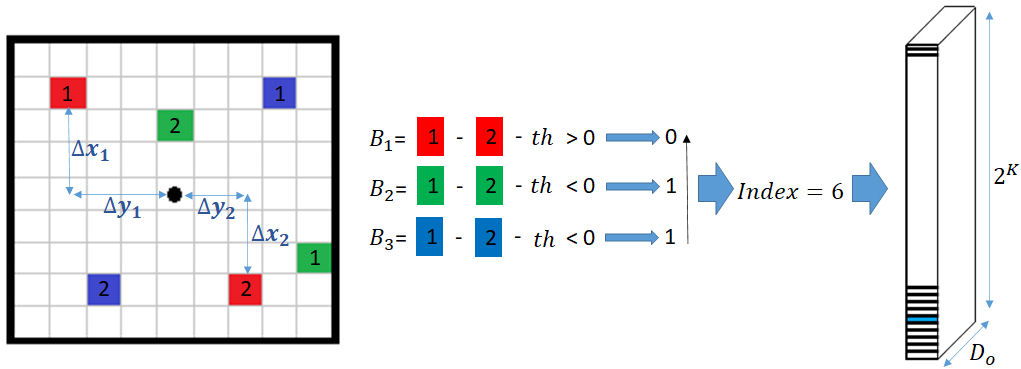
Figure 1: A Convolutional Table (CT) with a word calculator of three bits operating on a 2D input tensor. Each bit-function is given by two pixels whose difference is compared to a threshold (colored in red, green, and blue). The word computed by the three bits, ’110’ = 6, is used to access the $6^{th}$ entree in the voting table, thus computing an output vector $\in\mathbb{R}^{D_{o}}$.

III Convolutional Table Transform

A convolutional table is a transformation accepting a representation tensor $T^{in}\in\mathbb{R}^{H_{i}\times W_{i}\times D_{i}}$ and outputting a representation tensor $T^{out}\in\mathbb{R}^{H_{o}\times W_{o}\times D_{o}}$, where $H_{i},H_{i}$ and $W_{i},W_{0}$ are the spatial dimensions, while $D_{i}$, $D_{o}$ are the representation’s dimensionality for the input and output tensors, respectively. Formally, it is the tuple $(B,W)$, where $B$ is a word calculator, and $W$ is a voting table. A word calculator $B$ is a feature extractor applied to a patch, returning a $K$-bit index, such that $B:\mathbb{R}^{l\times l\times D_{i}}\rightarrow\{0,1\}^{K}$, where $l$ is the patch size. The voting table $W\in M^{{}_{2^{K}\times D_{o}}}$ contains all possible $2^{K}$ outputs as rows, each being a vector $\in\mathbb{R}^{D_{o}}$.

The index is computed by sequentially applying $K$ bit-functions $\{B^{k}\}_{k=1}^{K}$, each computing a single bit of the index. Let $P=(p_{x},p_{y})\in\mathbb{R}^{H_{i}\times W_{i}}$ be a location in $T^{in}$. We denote by $B(P;\Theta)=(B^{1}(P;\Theta^{1}),...,B^{K}(P,\Theta^{K}))$ the index computed for the patch centered at location $P$. Here $\Theta=(\Theta^{1},...,\Theta^{K})$ are the word calculator parameters, with $\Theta^{k}$ explicitly characterized below. The functions $B^{k}(P;\Theta^{k})\in\{0,1\}$ (dependence on $T^{in}$ is omitted for notation brevity) are computed by thresholding at $0$ the simple smooth functions $b^{k}(P;\Theta^{k})$ of a few input pixels. (i.e., $B^{k}(P;\Theta)=Q\left(b^{k}(P;\Theta^{k})\right)$ with $Q(\cdot)$ being the Heaviside function). Bit functions $b^{k}$ are the thresholded differences between two locations:

$$b^{k}\left(P;\Theta_{k}\right) = T^{in}\left(p_{x}+\Delta x_{1}^{k},p_{y}+\Delta y_{1}^{k},c^{k}\right)$$

$$-T^{in}\left(p_{x}+\Delta x_{2}^{k},p_{y}+\Delta y_{2}^{k},c^{k}\right)-th^{k},$$

where the learned parameters $\Theta^{k}$, define the compared locations $(\Delta x_{1}^{k},\Delta y_{1}^{k},c^{k})$ and $(\Delta x_{2}^{k},\Delta y_{2}^{k},c^{k})$, and the margin threshold $th^{k}$. $th^{k}$ is the learnable scalar margin threshold for comparing two locations within the patch corresponding to the $k$’th bit. The codeword computed by the word calculator is used as an index to the voting table to retrieve $W(B(P;\Theta),:)\in\mathbb{R}^{D_{o}}$ for location $P$. Figure 1 depicts the convolutional table operation at a single location. A CT (using padding= ‘same’ and stride=$1$) applies the operation defined above at each position $P\in\mathbb{R}^{H_{i}\times W_{i}}$ of the input tensor to obtain the corresponding output tensor column. Same as in convolutional layers, padding can be applied to the input for computations at border pixels, and strides may be used to reduce the spatial dimensions of the output tensor. A CT layer includes $M$ convolutional tables $\{(B_{m},W_{m})\}_{m=1}^{M}$ whose outputs are summed:

$$T^{out}[P, : ]=\sum_{m=1}^{M}W_{m}[B_{m}(T_{N(P)}^{in}),~{}:~{}],$$ (2)

$$B_{m} = \{B^{k}\}_{k=1}^{K}$$

The operation of a CT layer is summarized in Algorithm 1. Essentially, it applies a fern ensemble at each location, summing the output vectors from the ensemble’s ferns. A CT network stacks multiple CT layers in a cascade or graph structure, similar to stacking convolutional layers in standard CNNs.

Algorithm 1 Convolutional Table Layer

1:INPUT: A tensor $T^{in}\in\mathbb{R}^{H_{i}\times W_{i}\times D_{i}}$,transformation parameters $\{(\Theta^{m},W^{m})\}_{m=1}^{M}$

2:OUTPUT: An Output tensor $T^{out}\in\mathbb{R}^{H_{o}\times W_{o}\times D_{o}}$

3:Initialization: $T^{out}=0$, $\{(\Theta^{m},W^{m})\}_{m=1}^{M}\sim\mathcal{N}(0,\sigma^{2}=1)$

4:for $P\in\{1,..,H_{i}\}\times\{1,..,W_{i}\}$  do $\triangleright$ All pixel locations

5:     for $m=1,..,M$ do $\triangleright$ All CT tables

6:         Compute $B_{m}(P;\Theta^{k,m})\in{\{0,1\}}^{K}$ $\triangleright$ Eq. III

7:         $T^{out}[P,:]=T^{out}[P,:]+W^{m}[B_{m}(P;\Theta^{k,m}),:]$ $\triangleright$ Eq. 2

8:     end for

9:end for

10: Return $T^{out}$

IV Computational complexity

Let the input and output tensors be $T^{in}\in\mathbb{R}^{H_{i}\times W_{i}\times D_{i}}$ and $T^{out}\in\mathbb{R}^{H_{o}\times W_{o}\times D_{o}}$, respectively, where the dimensions are the same as in Section III, and let $l\times l$ be the filter’s support. For a convolution layer, the number of operations per location is $C_{CNN}=l^{2}D_{i}D_{o}$, since it computes $D_{o}$ inner products at the cost of $l^{2}D_{i}$ each. For a CT layer with $M$ CTs and $K$ bits in each CT, the cost of bits computation is $MKC_{b}$, with $C_{b}$ being the cost of computing a single bit-function. The voting cost is $MD_{o}$, since we add the vectors $\in\mathbb{R}^{MD_{o}}$ to get the result. Thus, the complexity of a CT layer is $C_{CT\;}=M(C_{b}\cdot K+D_{o})$.

It follows that the computational complexity of a CT is independent of the filter size $l$. Hence, it allows agglomerating evidence from large spatial regions with no additional computational cost. To compare CNN and CT complexities, assume that both use the same representation dimension $D_{i}=D_{o}=D$. The relation between the total number of bit-functions $MK$ and $D$ depends on whether each bit-function uses a separate dimension, or the dimensions are reused by multiple bit-functions. For a general analysis, assume each dimension is reused by $R$ bit-functions, such that $D=MK/R$ (in our experiments $R\in[1,3]$). Thus, the ratio of complexities between CNNs and CT layers with the same representation dimension $D$ is

$$\frac{C_{CNN}}{C_{CT\;}}=\frac{l^{2}D^{2}}{M(C_{b}\cdot K+D)}=\frac{l^{2}D^{2}}{C_{b}DR+\frac{D^{2}R}{K}}\approx\frac{Kl^{2}}{R},$$ (3)

where the last approximation is true for large $D$, and the quadratic terms in $D$ are dominant. The computation cost of computing a single bit function, $C_{b}$, is defined as the number of operations required to perform a single comparison operation between two locations within the patch size. This computation is described in equation III and involves four additions of the offsets of $\Delta_{x}$, $\Delta{y}$, and a subtraction of the threshold, $th^{k}$. This results in a total of five operations. Additionally, load operations are required for the two relevant memory locations and their two base addresses, bringing the total number of operations to nine. Although the most stringent count does not exceed 10 operations, for simplicity, we set $C{b}$ to 10. The ratio of complexities between CNNs and CT layers in Eq. 3 suggests there is the potential for acceleration by more than an order of magnitude for reasonable choices of parameter values. For example, using $l=3$, $K=8$, and $R=2$ results in a $36$ $\times$ acceleration. Although the result of this analysis is promising, several lower-level considerations are essential to achieve actual acceleration. First, operation counts translate into actual improved speed only if the operations can be efficiently parallelized and vectorized. In particular, vectorization requires contiguous memory access in most computations. The CT transformation adheres to these constraints. Contrary to trees, bit computations in ferns can be vectorized over adjacent input locations as all locations use the same bit-functions, and the memory access is contiguous. The voting operation can be vectorized over the output dimensions. This implementation was already built and has been shown to be highly efficient for flat CT classifiers [24]. Although a CT transformation uses a ‘random memory access’ operation when the table is accessed, this random access is rare: there is a single random access operation included in the $(C_{b}\cdot K+D_{o})$ operations required for a single fern computation. Another important issue is the need to keep the model’s total storage size within reasonable bounds to enable its memory to be efficiently accessed in a typical $L_{2}$ cache. For example, a model consisting of $50$ layers, wherein $M=10$ ferns, $K=6,$ and $D=60$, have a total size of $1.92MB$ when the parameters are stored in $8$-bit precision.

V CT capacity and expressiveness

In this section, we present two analytic insights that indicate the feasibility of deep CT networks and their potential advantages. In Section V-A the capacity of a fern is shown to be $\Omega(2^{K})$ with $O(K)$ computational effort, providing a much better capacity:compute ratio than a linear convolution. In Section V-B a network of two fern layers is shown to be a universal approximation, similarly to known results on neural networks. In the analysis, we consider a simplified non-convolutional setting, with an input vector $X\in[0,1]^{d}$, and a non-convolutional fern ensemble classifier. Furthermore, simple bit-functions of the form $B^{k}(X)=Q\left((-1)^{s^{k}}(X[I^{k}]-t^{k})\right)$ are considered, where $s^{k}\in\{0,1\},~{}I^{k}\in{1,..,d}~{},t^{k}\in[0,1]$. These simple bit-functions just compare a single entry to a threshold.

V-A Capacity:Compute ratio

The following lemma characterizes the capacity of a single fern in VC-dimension terms.

Lemma 1

Define the hypothesis family of binary classifiers based on a single $K-bit$ fern $H=\{f(X)=sign(W(B(X))):B={\{(s^{k},I^{k},t^{k})\}}_{k=1}^{K},W\in R^{2^{K}}\}$. For $K\geq 4$ and $log_{2}(d)<K\leq d$ its VC-dimension is

$$2^{K}\leq VC-dim(H)\leq K2^{K}$$ (4)

Proof:

Since we only consider the sign of the chosen table entry $W(B(X))$, we may equivalently consider the family of classifiers $f(X)=W(B(X))$ for $W\in{\{-1,1\}}^{2^{K}}$.

Lower bound: Consider a sample containing points on the $d$-dimensional cube

$$S=\{P_{c}=(-1^{c_{1}},...-1^{c_{K}}):~{}c=(c_{1},..,c_{K})\in\{0,1\}^{K}~{}\}.$$ (5)

It follows that this sample can be shattered by the binary fern family. We may choose the bit functions $b^{k}(X)=Q(X[k])$. Assume an arbitrary label assignment $l$, i.e. for each example $P_{c}$ we have $l(P_{c})=y_{c}$ with $y_{c}$ arbitrarily chosen in $\{-1,1\}$. By definition, for each $c$ and $k$, we have $b^{k}(P_{c})=\{-1\}^{c_{k}}=P_{c}[k]$. Since any two points $P_{c_{1}},P_{c_{2}}$ differ by at least a single dimension, they will have at least different bits in a single bit function. Hence, the $2^{K}$ points are mapped into the $2^{K}$ different cells of $W$. By choosing $W[c]=y_{c}$ we may get the desired labeling $l$. Therefore, $S$ is shattered, showing $VCdim(H)\geq 2^{K}$.

Upper Bound: Assume $K\geq 4$ and $log_{2}(d)<K\leq d$. We compute an upper bound on the number of possible labels (label vectors) enabled by the binary fern family on a sample of size $n$, and show it is smaller than $2^{n}$ for $n=K2^{K}$.

For a $K$-bit fern, there are $d^{K}$ ways to choose the input dimension of the $K$ bit-functions (one dimension per function). For each bit-function, once the input dimension $I$ is chosen, we may re-order the examples according to their value in dimension $I$, i.e., $X_{1}[I]\leq X_{2}[I]...\leq X_{n}[I]$. Non-trivial partitions of the sample, i.e. partitions into two nonempty sets, are introduced by choosing the threshold $t$ in $(X_{1}[I],X_{n}[I])$, and there are at most $n-1$ different options. Including the trivial option of partitioning $S$ into $S$ and $\Phi$, there are $n$ options.

Consider the number of partitions of the examples into $2^{K}$ cells, which are made possible using $K$ bit-functions. Two different partitions must differ w.r.t. the induced partition by a single bit-function choice, at least. Hence, their number is bounded by the number of ways to choose the bit-function partitions, which is $d^{K}n^{K}$ at most, according to the above considerations. For each such partition into $2^{K}$ cells, $2^{K}$ different classifiers can be defined by choosing the table entries $\{W[c]\}_{c=0}^{2^{K}-1}$. Hence, the total number of possible different fern classifiers for $n$ points is bounded by $(dn)^{K}2^{2^{K}}$. When this bound is lower than $2^{n}$, the sample cannot be shattered. Thus, we solve the problem

$$(dn)^{K}2^{2^{K}}<2^{n}$$ (6)

and

$$2^{K}+Klog_{2}d+Klog_{2}n<n.$$ (7)

By choosing $n=K2^{K}$ it follows that Eq. 7 is satisfied since

$$2^{K}+Klog_{2}d+Klog_{2}K+K^{2}\\ <2^{K}+3K^{2}\leq 2^{K}+(K-1)2^{K}\leq K2^{K}$$ (8)

For the second inequality we used $log_{2}d<K$ (assumed), and for the third we used the inequality $3K^{2}\leq(K-1)2^{K}$ which holds for $K\geq 4$.    

Results similar to the Lemma 1 were derived for trees [30, 45], and the lemma implies that the capacity of ferns is not significantly lower than that of trees. To understand its implications, compare such a single-fern classifier to a classifier based on a single dot-product neuron, i.e., a linear classifier. A binary dot-product neuron with $d=K$ input performs $O(K)$ operations to obtain a VC dimension of $O(K)$. The fern also performs $O(K)$ computations, but the response is chosen from a table of $2^{K}$ leaves, and the VC dimension is $\Omega(2^{K})$. The higher (capacity):(computational-complexity) ratio of ferns indicates that they can compute significantly more complex functions than linear neurons using the same computational budget.

V-B CT networks are universal approximators

The following theorem states the universal approximation capabilities of a $2$-layer CT network. It resembles the known result for two-stage neural networks [14].

Theorem 1

Any continuous function $f:[0,1]^{d}\rightarrow[0,1]$ can be approximated in $L_{\infty}$ using a two-layer fern network with $K=1$ in all ferns.

Proof:

The core of the proof is to show that by using $2K$ 1-bit ferns at the first layer, a second layer fern can create a function with an arbitrary value inside a hyper-rectangle of choice, and zero outside the rectangle. Since sums of such ‘step functions’ are dense in $C[0,1]$, so are two-layer fern networks.

Let $R=[a_{1},b_{1}]\times[a_{2},b_{2}]...\times[a_{d},b_{d}]$ be a hyper rectangle in $R^{d}$ and $v\in R$ a scalar value. A rectangle function $s(x;v,R):[0,1]^{d}\rightarrow R$ is defined as $v\cdot 1_{x\in R}$, i.e. a function whose value is $f(x)=v$ for $x\in R$ and $0$ otherwise. Define the family of step functions

$$G=\{g:[0,1]^{d}\rightarrow[0,1]:g(x)=\sum_{p=1}^{P}s(x;v_{p},R_{p})\}.$$ (9)

It is known that $G$ is dense in $(C[0,1]^{d})$ (from the Stone-Weierstrass theorem, see e.g. [10] ). We will show that the family of $2$-layer CT networks includes this set.

Let $s(v,R)$ be an arbitrary rectangle function. For each dimension $i=1,..,d$, define the following two bit-functions: $L_{i}(x)=Q(x-a_{k})$ and $R_{i}(x)=Q(-(x-b_{k}))$. Denote these bit-functions by $B_{(R)}^{j}$ for $j=1,..,2d$. By construction, ${\{B_{R}^{j}\}}_{j=1}^{2d}$ characterize the rectangle

$$x\in R\iff\forall j=1,..,2d~{}~{}~{}B_{R}^{j}(x)=1.$$ (10)

Equivalently, we have $x\in R$ iff $\sum_{j=1}^{2d}B_{R}^{j}(x)>2d-\frac{1}{2}$. Given a function $g(x)=\sum_{p=1}^{P}s(x;v_{p},R_{p})$ to implement, we define at the first layer $P$ sets of ferns. Fern set $p$ contains $2d$ ferns, denoted by $F_{p}^{j}$, with a single bit-function each, and the bit-function of $F_{p}^{j}$ is $B_{R_{p}}^{j}$. The output dimension of the first layer is $P$. The weight table $W_{p}^{j}\in M_{2\times P}$ of $F_{p}^{j}$ is defined by

$$W_{p}^{j}[i,l]=\begin{cases}1&i=1,l=p\\ 0&otherwise\end{cases}.$$ (11)

The output vector of a layer is the sum of all ferns $Y=\sum_{p^{\prime}=1}^{P}\sum_{j=1}^{2d}W_{p^{\prime}}^{j}[B_{R_{p^{\prime}}}^{j}(x),:].$ By construction we have

$$Y[p] = \sum_{p^{\prime}=1}^{P}\sum_{j=1}^{2d}W_{p^{\prime}}^{j}[B_{R_{p}^{\prime}}^{j}(x),p]$$

$$= \sum_{j=1}^{2d}W_{p}^{j}[B_{R_{p}}^{j}(x),p]=\sum_{j=1}^{2d}B_{R_{p}}^{j}(x).$$

The second equality holds since $W_{p^{\prime}}^{j}[i,p]$ only differs from zero for $p=p^{\prime}$. The last equality is valid since $W_{p}^{j}[i,p]=i$ for $i=0,1$. We hence have $Y[p]=2d>2d-\frac{1}{2}$ for $x\in R_{p}$, that has lower values anywhere else.

The second layer of ferns contains $P$ ferns, each with a single bit and a single output dimension. For fern $p$, we define the bit-function $B_{p}^{(2)}(Y)=Q(Y[p]-(2d-\frac{1}{2}))$ which fires only for $x\in R_{p}$ and the table $W_{p}^{(2)}=[0,v(p)]$. The output unit $U$ computes

$$U = \sum_{p=1}^{P}W_{p}^{(2)}[B_{p}^{(2)}(x)]$$

$$= \sum_{p=1}^{P}v(p)\cdot B_{p}^{(2)}(x)=\sum_{p=1}^{P}v(p)\cdot 1_{x\in R_{p}}.$$

Therefore, $U$ implements the function $g(x)$, which completes the proof.    

VI Training with soft Convolutional Tables

Following Eq. III, $B^{k}\left(P;\Theta_{k}\right)=Q(b^{k}(P;\Theta_{k}))$ does not enable gradient-based optimization, as the derivative of the Heaviside function $Q(\cdot)$ is zero almost anywhere. We suggest a soft version of the CT in Section VI-A that enables gradient-based optimization, and discuss its gradient in Section VI-B.

VI-A A soft CT version

To enable gradient-based learning, we suggest replacing the Heaviside function during optimization with a linear sigmoid $q(x;t)$ for $t>0$:

$$q(x;t)=min(max(~{}(t+x)/2t~{},0),1).$$ (14)

$q(x;t)$ is identical to the Heaviside function for $x\gg 0$ and is a linear function in the vicinity of $x=0$. It has a nonzero gradient in $[-t,t]$, where $t$ is a hyperparameter controlling its smoothness. For low $t$ values, we have $q(x;t)\underset{t\rightarrow 0}{\rightarrow}Q(x)$. Moreover, we have $q(x;t)+q(-x;t)=1$. Thus, it can be interpreted as a pseudo-probability, with $q(x)$ estimating the probability of a bit being $1$ and $q(-x)$ the probability of being 0.

Following Section III, a word calculator $B$ maps a patch $P$ to a single index or equivalently to a one-hot vector (row) in $R^{2^{K}}$. Denote the word calculator in the latter view (mapping into $R^{2^{K}})$ by $\vec{B}(P;\Theta)$. Given this notation, the CT output is given by the product $\vec{B}\cdot W$. Hence, extending the word calculator to a soft function in $R^{2^{K}}$, with dimension $b\in\{0,..,2^{K}-1\}$ measuring the activity of the word $b$, provides a natural differentiable extension of the CT formulation. For an index $b,$ define the sign of its $k^{th}$ bit by $s(b,k)\triangleq(-1)^{(1+u(b,k))}$, where $u(b,k)$ denotes the $k^{th}$ bit of the index $b$ in its standard binary expansion, such that

$$s(b,k)=\left\{\begin{tabular}[]{rl}$1$&bit $k=1$\\ $-1$&bit $k=0$\end{tabular}\right..$$ (15)

The activity level of the word $b$ in a soft word calculator is defined by

$$\vec{B}^{s}(P;\Theta)[b]=\prod_{k=1}^{K}~{}q(~{}s(b,k)\cdot b_{k}(P;\Theta_{k});t~{}).$$ (16)

Intuitively, the activity level of each possible codeword index $b$ is a product of the activity levels of the individual bit-functions in the directions implied by the codeword bits. Marginalization implies that $\sum_{b=0}^{2^{K}-1}\vec{B}^{s}(P)[b]=1$, and hence the soft-word calculator defines a probability distribution over the possible $K$-bit words. Soft CT is defined as natural extension $\vec{B}^{s}W$. Note that as $t\rightarrow 0$, the sigmoid $q(x;t)$ becomes sharp, $\vec{B}^{s}$ becomes a one-hot vector and the soft CT becomes a standard CT as defined in Section III, without any inner products.

Soft CT can be considered as a consecutive application of two layers: a soft indexing layer $\vec{B}^{s}$ followed by a plain linear layer (though sparse if most of the entries in $\vec{B}^{s}$ are zero). Since CT is applied to all spatial locations on the activation map, the linear layer $W$ corresponds to a $1\times 1$ convolution. We implemented a sparse $1\times 1$ convolutional layer operating on a sparse tensor $\mathbf{x\in}R^{H\times W\times 2^{K}}$ and outputting a dense tensor $\mathbf{y\in}$ $R^{H\times W\times D_{o}}$.

VI-B Gradient computation and training

Since applying the soft CT in a single position is $W\cdot B^{s}(P;\Theta),$ with $W$ being a linear layer, it suffices to consider the gradient of $\vec{B}^{s}(P;\Theta)$. Denote the neighborhood $l\times l$ of the location $P$ in $T^{in}$ by $T_{N(P)}^{in}$. Taking into account a single output variable $b$ at a time, the gradient with respect to the input patch $T_{N(P)}^{in}$ is given by

$$\frac{\partial\vec{B}^{s}(P)[b]}{\partial T_{N(P)}^{in}}=\sum_{k}\frac{\partial\vec{B}^{s}(P)[b]}{\partial b_{k}(P;\Theta_{k})}\cdot\frac{\partial b_{k}(P;\Theta_{k})}{\partial T_{N(P)}^{in}},$$ (17)

with a similar expression for the gradient with respect to $\Theta$. For a fixed index $k$, the derivative $\frac{\partial\vec{B}^{s}(P)[b]}{\partial b_{k}(P;\Theta_{k})}$ is given by

$$\frac{\partial\vec{B}^{s}(P)[b]}{\partial b_{k}(P;\Theta_{k})}=\\ \prod_{j\neq k}~{}q(s(b,j)b_{j}(P;\Theta_{j});t)\frac{\partial q(s(b,j)b_{j}(P;\Theta_{j});t)}{\partial b_{k}(P;\Theta_{k})}=\\ \frac{\vec{B}^{s}(P)[b]\cdot t^{-1}\cdot 1_{|b_{k}|<t}\cdot s(b,k)}{2q(~{}s(b,k)\cdot b_{k}(P;\Theta_{k}))}.~{}~{}~{}$$ (18)

The derivative is non-zero when the word $b$ is active (i.e. $\vec{B}^{s}(P)[b]>0$), and the bit-function $b_{k}(P)$ is in the dynamic range $-t<b_{k}(P)<t$.

To further compute the derivatives of $b_{k}(P)$ with respect to the input and parameters ($\frac{\partial b_{k}(P;\Theta_{k})}{dT_{N(P)}^{in}}$ and $\frac{\partial b_{k}(P;\Theta_{k})}{d\Theta}$, respectively), we first note that the forward computation of $b_{k}(P)$ estimates the input tensor at fractional spatial coordinates. This is due to the fact that the offset parameters $\Delta x_{1},\Delta y_{1},\Delta x_{2},\Delta y_{2}$ are trained with gradient descent, which requires them to be continuous. We use bilinear interpolation to compute image values at fractional coordinates in the forward inference. Hence, such bilinear interpolation (of spatial gradient maps) is required for gradient computation. For instance, $\frac{\partial b_{k}(P)}{\partial\Delta x_{1}^{k}}$ is given by

$$\frac{\partial b_{k}(P)}{\partial\Delta x_{1}^{k}}=\frac{\partial T^{in}\left(p_{x}+\Delta x_{1}^{k},p_{y}+\Delta y_{1}^{k},c\right)}{\partial\Delta x_{1}^{k}}\\ =\frac{\partial T^{in}(:,:,c)}{\partial x}[(p_{x}+\Delta x_{1}^{k},p_{y}+\Delta y_{1}^{k})],$$ (19)

where $\frac{\partial T^{in}(:,:,c)}{\partial x}$ is the partial x-derivative of the image channel $T^{in}(:,:,c)$, that is estimated numerically and sampled at $\left(x,y\right)=(p_{x}+\Delta x_{1}^{k},p_{y}+\Delta y_{1}^{k})$ to compute Eq. 19. The derivatives with respect to other parameters are computed in a similar way. Note that the channel index parameters $c^{k}$ are not learnt - these are fixed during network construction for each bit-function. As for $\frac{\partial b_{k}(P;\Theta_{k})}{dT_{N(P)}^{in}}$, by considering Eq. III, it follows that $b_{k}(P;\Theta_{k})$ only relates to two fractional pixel locations: $\left(p_{x}+\Delta x_{1}^{k},p_{y}+\Delta y_{1}^{k}\right)$ and $\left(p_{x}+\Delta x_{2}^{k},p_{y}+\Delta y_{2}^{k}\right)$. This implies that a derivative with respect to eight pixels is required, as each value of a fractional coordinates pixel is bilinearly interpolated using its four neighboring pixels in integer coordinates.

The sparsity of the soft word calculator (both forward and backward) is governed by the parameter $t$ of the sigmoid in Eq. 14, which acts as a threshold. When $t$ is large, most of the bit-functions are ambiguous and soft i.e., not strictly $0$ or $1$, and the output will be dense. We can control the output’s sparsity level by adjusting $t$. In particular, as $t\rightarrow 0,$ the bit-functions become hard, and $B^{s}(P)$ converges toward a hard fern with a single active output word. While a dense flow of information and gradients is required during training, fast inference in test time requires a sparse output. Therefore, we introduce an annealing scheduling scheme, such that $t$ is initiated as $t\gg 0$, set to allow a fraction $f$ of the values of the bit functions to be in the ‘soft zone’ $[-t,t]$. The value of $t$ is then gradually lowered to achieve a sharp and sparse classifier towards the end of the training phase.

VII Experimental Results

We experimentally examined and verified the accuracy and computational complexity of the proposed CT scheme, applying it to multiple small and medium image datasets, consisting of up to 250K images. Such datasets are applicable to IoT and non-GPU low compute devices. We explored the sensitivity of CT networks to their main hyperparameters in Section VII-A. To this end, we studied the number of ferns $M$ and the number of bit functions per fern $K$, and the benefits of distillation as a CT training technique. We then compared our CT-based architectures to similar CNN classes. Such a comparison is nontrivial due to the inherent architectural differences between the network classes. Thus, in Section VII-B we compared Deep CT to CNNs with similar depth and width, that is, the number of layers and maps per layer. The comparison focuses on efficient methods suggested for network quantization and binarization, since the CT framework uses similar notions. In Section VII-C the CT is compared to CNN formulations with comparable computational complexity, i.e., similar number of MAC (Multiply-ACcumulate) operations. We compared CT with CNN architectures specifically designed for inference efficiency, such as MobileNet [35] and ShuffleNet [29]. The comparison was applied by studying the speed:error and speed:error:memory trade-offs of the different frameworks. Finally, to exemplify the applicability of Deep CT to low-power Internet-of-Things (IoT) applications and larger datasets (250K images), it was applied to IoT-based face recognition in Section VII-D.

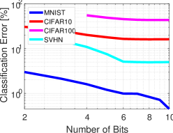
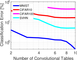
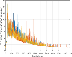
Figure 2: Hyperparameters study on MNIST, CIFAR10, CIFAR100, and SVHN datasets. (a) Deep CT network error Vs. the number of bits $K$ in a log-log plot. In all layers, the number of convolutional tables $M$ was fixed to $10$. (b) Deep CT network error Vs. the number of convolutional tables $M$ in a log-log plot, for a fixed number of bits $K=10$. (c) The average number of active words per CT was evaluated using the CIFAR-10 dataset and plotted against the training batch index. Each convolution table is represented by a different color: yellow, blue, and red. As expected, the number of active words decreases during the training process due to the annealing mechanism and eventually converges to a single active word.

The proposed novel CT layer does not use standard CNN components such as activations, convolutions, or FCs. Thus, the Deep CT word calculator layer and the sparse voting table layer were implemented from scratch, in unoptimized C, compiled as MEX files, and applied within a Matlab implementation. Our experiments were carried out on the same computer using CPU-only implementations for all schemes.

Similar to other inherently novel layers, such as Spatial Transformer Networks, it is challenging to implement a converging end-to-end training process. To facilitate the convergence of the proposed scheme, a three-phase training scheme was applied. First, the lower half of the CNN (layers #1-#6 in Table VIII) was trained, by adding the Average Pooling (AP), Softmax (SM) and Cross Entropy (CE) layers on top of layer #6. Then, the full architecture was trained with layers #1 through #6 frozen. Finally, following Hinton et al. [15], we unfroze all layers and refined the entire network using a distillation-based approach. The CT was trained to optimize a convex combination of CE loss and Kullback-Leibler divergence with respect to the probabilities induced by a teacher CNN. The temperature parameter was initially set at $t=4$ and gradually annealed to $t=1$ toward the end of the training. All Deep CT networks were trained from scratch using random Gaussian initialization of the parameters.

VII-A Hyperparameters sensitivity

The expressive power of the Deep CT transformation is related to the number of CTs per layer $M$, and the number of bit-functions $K$ used in each CT. We tested the sensitivity of the Deep CT network to these parameters and the suggested annealing schedule. These experiments applied CT networks with four layers to the SVHN, CIFAR-10, and CIFAR-100 datasets, and two layers to the MNIST dataset. The Networks are similar to those shown in the appendix, in Tables VI and VII. We used a fixed patch size $l=5$ and input and output dimensions of $D_{i}=D_{o}=32$, respectively. It is best to apply CT networks with a patch size larger than the kernel size of CNN-based networks, since CT patches are sparsely represented. Comparatively, CNN complexity is quadratic with respect to patch size, while CT networks’ computational complexity is independent of patch size.

The classification errors with respect to the bit-functions $K$ (for a fixed $M$), and the number of CTs $M$ (for a fixed $K$) are shown in Figs. 2a and  2b, respectively. For most datasets, there is a range in which the error exponentially decreases as the number of network parameters increases, while the accuracy improvement saturates for $M>8$ and $K>8$ for the deeper networks (datasets other than MNIST).

Figure 2c shows the average number of active words in a convolutional table as a function of the training time for CIFAR-10. The fraction $f$ of ambiguous bits (bits whose value is not set to either $0$ or $1$) was started at $0.2$ and was gradually reduced exponentially, while the sigmoid threshold $t$ was adjusted periodically according to the required $f$. In our experiments, the sigmoid threshold was set to $t=0.5$. The number of active words per CT is thus gradually reduced and converged to a single active word in the final classifier. The CNN with four layers obtained a test error of 12.55%, compared to 12.49% with the same architecture without annealing. Therefore, annealing-based training led to a sparser classifier without significantly degrading the classification accuracy.

To establish the best hyperparameters, additional experiments were carried out for multiple M and K combinations around $M=8,K=8$. The experiments were conducted using the CIFAR-10 dataset, and the CT networks having four and six layers, detailed in Tables VII and II, respectively. In addition, we examined training with and without distillation from a teacher. The $M=8,K=8$ configuration was found to be the most accurate. Distillation was found to be beneficial, providing accuracy improvements of $1\%-2\%$.

$\mathbf{K}$	$\mathbf{M}$	Layers#	Distil	Error [%]
9	8	6	No	11.31
8	9	6	No	12.31
8	8	6	No	11.05
7	8	6	No	13.93
8	7	6	No	13.34
8	8	6	Yes	10.25
9	8	4	No	12.88
8	9	4	No	13.05
8	8	4	No	12.49
7	8	4	No	13.25
8	7	4	No	12.90
8	8	4	Yes	10.91

TABLE I: Joint hyperparameters tuning for the four and six layers CT networks described in Tables VII and II. $M$ and $K$ denote the Convolution tables’ size and the number of bits, respectively.

Deep CT		Parameters	Output	Convolution	Parameters	Output
Layer		$l,K,M,D_{o}$		Layers
1	CT Layer 1	$7,8,8,32$	$26\times 26\times 32$	Conv,ReLU	$l=3,D_{o}=32$	$30\times 30\times 32$
2	Average Pooling	$l=3$	$24\times 24\times 32$	Max Pooling	$l=3,Stride=2$	$14\times 14\times 32$
3	CT Layer 2	$5,8,8,32$	$20\times 20\times 32$	Conv,ReLU	$l=3,D_{o}=32$	$12\times 12\times 32$
4	Average Pooling	$l=3$	$18\times 18\times 32$	Max Pooling	$l=2$	$11\times 11\times 32$
5	CT Layer 3	$5,8,8,64$	$14\times 14\times 64$	Conv,ReLU	$l=3,D_{o}=64$	$9\times 9\times 64$
6	Average Pooling	$l=3$	$12\times 12\times 64$	Max Pooling	$l=2$	$8\times 8\times 64$
7	CT Layer 4	$5,8,8,128$	$8\times 8\times 128$	Conv,ReLU	$l=3,D_{o}=128$	$6\times 6\times 128$
8	Average Pooling	$l=2$	$7\times 7\times 128$	Max Pooling	$l=2$	$5\times 5\times 128$
7	CT Layer 5	$3,8,8,64$	$5\times 5\times 64$	Conv,ReLU	$l=3,D_{o}=64$	$4\times 4\times 64$
8	Average Pooling	$l=2$	$4\times 4\times 64$	Max Pooling	$l=2$	$3\times 3\times 64$
9	CT Layer 6	$3,8,8,10$	$2\times 2\times 10$	Conv,ReLU	$l=3,D_{o}=10$	$1\times 1\times 10$
10	Average Pooling	$l=2$	$1\times 1\times 10$	FC	$D_{o}=10$	$1\times 1\times 10$
11	SoftMax			SoftMax		$1$

TABLE II: The six-layer Deep CT and CNN networks applied to the CIFAR10, CIFAR100, and SVHN datasets. The CNN binarization schemes were applied to the CNN architecture, where $l$ and $K$ denote the patch size and the number of bits, $M$ is the number of convolutional tables and $D_{o}$ is the number of output maps.

Dataset	DeepCT	BC	XN	XN++	TABCNN	DSQ	DSQ	DSQ	Bi-Real	SLB	DeepCT	CNN
		[7]	[34]	[4]	[27]	[12] 2b	[12] 4b	[12] 6b	[28]	[42]	+ distil.
Two layers [%]
MNIST	0.35	0.61	0.51	0.39	0.49	0.41	0.38	0.36	0.36	0.37	0.39	0.334
Four layers [%]
CIFAR10	12.49	14.47	14.77	12.97	13.97	12.87	12.71	12.68	12.72	12.66	10.91	10.86
CIFAR100	39.17	50.27	47.32	41.03	45.32	40.14	40.05	39.96	39.97	39.55	37.12	36.81
SVHN	4.75	6.21	5.88	4.92	5.11	4.85	4.79	4.77	4.79	4.80	4.46	4.27
Six layers [%]
CIFAR10	11.05	12.56	12.91	11.88	12.13	11.35	11.27	11.14	11.19	11.16	10.25	9.88
CIFAR100	37.95	42.43	40.14	39	39.37	38.31	38.25	38.12	38.15	38.05	36.05	35.58
SVHN	4.12	4.95	4.54	4.25	4.28	4.21	4.18	4.15	4.17	4.25	3.96	3.77

TABLE III: Comparison of the classification error percentage. We compare the results for CNNs consisting of 2 layers (MNist) or 4 and 6 layers (other datasets). All quantized/binarized CNNs were derived by applying the corresponding quantization/binarization schemes to the baseline CNN having the same number of layers (Tables VI, VII and II). The most accurate results are marked in bold.

VII-B Accuracy comparison of low-complexity architectures

Although deep CT and CNN networks use very different computational elements, both use a series of intermediate representations to perform classification tasks. Hence, we consider CT and CNN backbone networks similar if they have the same number of intermediate representations (depth) and the same number of maps in each representation (width). In this section, we report experiments comparing CNN and CT networks that have identical configurations in these respects. Although the intermediate spatial tensors were chosen to be similar, we allowed for different top inference layers. Those were chosen to optimize the classification accuracy for each network class. Thus, the CNN-based networks used max-pooling and an FC layer, while the CT CNN only used an average pooling layer.

We compared the classification accuracy of CT networks to standard CNNs and contemporary low-complexity CNN architectures based on CNN binarization schemes. The methods we compared against include the BinaryConnect (BC)  [7] , XNOR-Net (XN) [34] , XNOR-Net++ (XN++)[4], Bi-Real Net (Bi-Real) [28], SLB [42] and TABCNN[27], using their publicly available implementations. These methods, [34] and [27] in particular, also encode the input activity using a set of binary variables. In contrast to our CT table-based approach, they use dense encodings and apply a binary dot-product to their encoded input. Finally, we applied the state-of-the-art Differentiable Soft Quantization (DSQ) scheme [12] to the conventional CNN to quantize it to 2, 4, and 6 bits.

All networks were applied to the MNIST [25], CIFAR-10 [21], CIFAR-100 [22], and SVHN [33] datasets. For the MNIST dataset, we applied CT networks and CNNs consisting of two layers, as this relatively small dataset did not require additional depth. For the other datasets, networks consisting of four and six layers were applied.

The architectures of the six-layer networks are detailed in Table II, and the architectures of the two and four layers used are detailed in the appendix in Tables VI and VII, respectively. The classification accuracy results are reported in Table III. On the left-hand side of the table, all methods are compared using the cross-entropy loss. The proposed CT networks outperformed the binarization and discretization schemes in all cases and were outperformed by conventional CNNs. In the right-hand column of the table, we show the results of a CT network using a distillation loss and a VGG16 [46] teacher network. These CT network improve the accuracy significantly further, and the margin of CNNs over them is also significantly smaller. Several key findings can be drawn from these results: First, the good accuracy of CT networks indicates that they can be trained using standard SGD optimization, such as CNNs, without significant overfitting. Second, the similar precision of the CT and CNN networks with a similar intermediate representation structure indicates that the accuracy is more dependent on the representation hierarchy structure than the particular computing elements used.

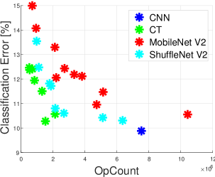
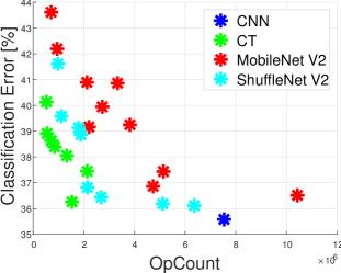
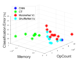
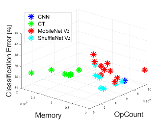
Figure 3: Performance trade-offs of the deep CT using an architectures of six-layers. (a) The Speed:Error trade-off for several families of models applied to the CIFAR-10 dataset. The models are based on the CNN in Table VII, CT networks, MobileNet V2 [35], and ShuffleNet V2 [29]. We considered architectures using up to $10^{7}$ operations. (b) Speed:Error trade-off on the CIFAR-100 dataset. (c) Speed:Error:Memory trade-off on CIFAR-10. (d) Speed:Error:Memory trade-off on CIFAR-100. CT-networks provide better Speed:Error trade-off in this domain while requiring additional memory. The speed is measured by the MACC operation count. The memory is given by the number of parameters, while the error is the classification percentage error.

Error	Speedup			Memory ratio
[%]	CT	[35]	[29]	CT	[35]	[29]
CIFAR-10
10.6	4.91	0.72	1.47	0.09	2.67	2.86
11.6	5.69	1.59	3.51	0.14	5.53	8.12
12.6	14.29	3.42	6.74	0.45	6.76	26.46
CIFAR-100
36.6	4.91	0.72	2.80	0.09	2.67	6.77
38.1	5.69	1.59	3.51	0.14	5.53	8.12
39.6	13.74	3.42	6.74	0.28	6.76	26.46

TABLE IV: Speed and memory trade-offs comparing the proposed CT, MobileNet2 [35] and ShuffleNet2 [29], using the CIFAR-10 and CIFAR-100 datasets. Each row relates to a particular classification percentage error and shows the corresponding speed and memory trade-offs. Speedup and memory ratios are computed by $\frac{R_{CNN}}{R_{Net}}$ where $R_{CNN}$ is the resources required by the baseline CNN, as in Table III, and $R_{Net}$ is the network’s requirements.

VII-C Trade-offs comparison: Accuracy, speed, and memory

We studied the Error:Speed and Error:Speed:Memory trade-offs enabled by the CT networks and compared them to those of contemporary state-of-the-art schemes. The experiments were conducted using the CIFAR10 and CIFAR100 datasets. Seven models of the CT network were trained, with operation count budgets $3.1X-12X$ lower than those of the baseline CNN in Table VII ($7.54\cdot 10^{6}$). Same as the baseline CNN, the CT models had six layers. The variations were derived by changing the hyperparameters $M$, $K$, and the number of channels at intermediate layers.

Dataset	Deep CT	BC	XN	TABCNN	DSQ 2 bits	DSQ 4 bits	DSQ 6 bits	MobileNet	ShuffleNet	CNN
CASIA 25K	87.21	85.36	86.286	86.95	87.05	87.15	87.19	87.20	87.186	89.96
CASIA 250K	90.66	87.95	88.35	88.89	90.06	90.27	90.35	90.63	90.54	93.25

TABLE V: The accuracy percentage of Deep CT, CNN, MobileNet V2 [35] and ShuffleNet V2 [29] when applied to subsets of the CASIA-WebFace dataset.

We compare the trade-off of the CT networks with those of the MobileNet V2 [35] and ShuffleNet V2 [29] efficient CNN architectures. The first is based on inverted bottleneck residual blocks, where depth-wise convolutions are performed on high-depth representations, and the second used blocks in which half of the channels are processed, followed by a channel shuffle operation. We used the code provided by the corresponding authors and adapted it to the relevant low-compute regime by adjusting their hyperparameters. For MobileNet, the networks were generated by adjusting the expansion parameter $t$ (Table 1 in [35]), the number of channels in intermediate representations, and the number of bottleneck modules in a block (between $1$ and $2$). For ShuffleNet, the networks were generated by changing the number of channels in the intermediate layers and the number of bottleneck modules in a block (between $1$ and $4$).

Error:Speed results are shown in Figs. 3a-b for CT networks and competing lean network approaches. These plots show that the proposed CT networks significantly outperform the baseline CNN and competing architectures. To enable a more explicit assessment, Table IV left-hand side shows the speedup achieved by the most efficient networks in each framework, for several error values on the CIFAR-10 and CIFAR-100 datasets. In the high-accuracy end, while losing at most $1\%$ error w.r.t. to the baseline CNN, the CT network enables $4.91X$ acceleration over the CNN and an acceleration of $1.75-6.8X$ over competing methods. When more significant errors are allowed ($2.7\%$ for CIFAR-10, $4\%$ for CIFAR-100), the CT networks provide accelerations of $13X-14X$ over the baseline CNN, significantly outperforming the $6.7X$ acceleration obtained by the best competitor [29]. The baseline CNN uses $7.54\cdot 10^{7}$ MACC operations, $181\cdot 10^{6}$ parameters, and obtains errors of $9.88$ and $35.58$ on CIFAR-10 and CIFAR-100, respectively. The tables for CIFAR-10 and CIFAR-100 are similar, as the same architectures are preferable for both datasets in each category of error and network type.

Figures 3c-d depict the Error:Speed:Memory trade-off for CT networks and other networks, using the CIFAR-10 and CIFAR-100 datasets, respectively. The memory requirements of the most efficient networks for each accuracy level are listed on the right-hand side of Table IV, as compression ratios with respect to the baseline CNN. Clearly, the better Error:Speed trade-off of the CT networks comes at the expense of a larger memory footprint (additional parameters). This is expected, as in CT transformations with memory-based retrieval replacing dot-product operations, the compute:memory ratio is much lower. For instance, in the high-accuracy regime, using the CIFAR-10 dataset allows a $4.9X$ speedup over the baseline CNN while requiring $10.7X$ more parameters. However, the size of excess memory can be controlled by limiting $K$ (for which the memory demand is exponential) to moderate values. Table IV shows that the fastest CT network enabling CIFAR-10 error of 12.6% provides an $14.3X$ acceleration while requiring only $2.2X$ additional parameters over the baseline CNN.

VII-D A face recognition test-case

We experimented with CT networks for face recognition using the CASIA-WebFace dataset [43]. Two datasets of $64\times 64$ extracted face images were formed. First, we randomly drew a subset of 50 classes (each with $5000$ images), 250K images overall, to evaluate the proposed CT on a large-scale dataset. We also randomly drew 50 identities and a class of negatives (not belonging to the 50 identities), each consisting of $500$ images. This exemplifies a typical IoT application, where face recognition is an enabler of personalized IoT services in smart homes, as well as security cameras. For both datasets, we trained a six-layer CT network and a CNN comparable in terms of the number of layers and intermediate tensor width. The architectures used are detailed in Table VIII in the appendix. The CT accuracy was compared to the baseline CNN, to the CNN versions produced by the compression techniques used in Section VII-B, and to the efficient CNN frameworks [35, 29] used in Section VII-C. To compare with the six layers CNN and CT networks, the MobileNet2 and ShuffleNet2 networks were constructed with six blocks: an initial convolution layer and a bottleneck block in the high resolution, followed by two bottleneck blocks in the second and third resolutions. The number of maps at each intermediate representation was identical to the widths used by the CT and CNN networks in Table VIII. The results are presented in Table V. With $25K$ and $250K$ data samples, the CT network outperformed all accelerated methods, with results comparable to MobileNet V2, and was only outperformed by conventional CNN. In particular, the $250K$ set results show that the CT can be effectively applied to large datasets.

VIII Summary and future work

In this work, we introduced a novel deep learning framework that utilizes indices computation and table access instead of dot-products. The experimental successful validation of our framework implies that both optimization and generalization are not uniquely related to the properties and dynamics of dot-product neuron interaction and that having such neuronal ingredients is an unnecessary condition for successful deep learning. Our analysis and experimental results show that the suggested framework outperforms conventional CNNs in terms of computational complexity:capacity ratio. Empirically, we showed that it enables improved speed:accuracy trade-off for the low-compute inference regime at the cost of additional processing memory. Such an approach is applicable to a gamut of applications that are either low-compute or are to be deployed on laptops/tablets that are equipped with large memory, but lack dedicated GPU hardware. Future work will extend the applicability of CT networks using an improved GPU-based training procedure. In this context, it should be noted that only basic CT networks were introduced and tested in this work, while competing CNN architectures enjoy a decade of intensive empirical research. The fact that CT networks were found competitive in this context is therefore highly encouraging. Combining CT networks with CNN optimization techniques (batch/layer normalization), regularization techniques (dropout), and architectural benefits (Residuals connections) is yet to be tested. Finally, to cope with the memory costs, methods for discretization/binarization of the model’s parameters should be developed, similarly to CNN discretization algorithms.

Deep CT		Parameters	Output	Convolution	Parameters	Output
Layer		$l,K,M,D_{o}$		Layer	$l,D_{o}$
1	CT Layer 1	$9,10,10,100$	$20\times 20\times 100$	Conv,ReLU	$l=5,D_{o}=100$	$24\times 24\times 100$
2	Average Pooling	$l=7$	$14\times 14\times 100$	Max Pooling	$l=5,Stride=2$	$10\times 10\times 100$
3	CT Layer 2	$9,10,10,10$	$6\times 6\times 10$	Conv,ReLU	$l=5,D_{o}=10$	$6\times 6\times 10$
4	Average Pooling	$l=6$	$1\times 1\times 10$	Max Pooling+FC	$l=6$	$1\times 1\times 10$
5	SoftMax		$1$	SoftMax		$1$

TABLE VI: The two-layers Deep CT and CNN networks applied to the MNIST dataset. $l$ and $K$ denote the size of the patch and the number of bits, $M$ is the number of convolutional tables and $D_{o}$ is the number of output maps.

IX Appendix A

The architectures used in Section VII-B for networks consisting of $2$ and $4$ layers are described in Tables VI and VII, respectively. The architectures used for CASIA-Webface data in Section VII-C are detailed in Table VIII.

Deep CT		Parameters	Output	Convolution	Parameters	Output
Layer		$l,K,M,D_{o}$		Layers
1	CT Layer 1	$7,8,8,32$	$26\times 26\times 32$	Conv,ReLU	$l=5,D_{o}=32$	$28\times 28\times 32$
2	Average Pooling	$l=3$	$24\times 24\times 32$	Max Pooling	$l=3,Stride=2$	$13\times 13\times 32$
3	CT Layer 2	$7,8,8,32$	$18\times 18\times 32$	Conv,ReLU	$l=3,D_{o}=32$	$11\times 11\times 32$
4	Average Pooling	$l=3$	$16\times 16\times 32$	Max Pooling	$l=3$	$9\times 9\times 32$
5	CT Layer 3	$7,8,8,64$	$10\times 10\times 64$	Conv,ReLU	$l=3,D_{o}=64$	$7\times 7\times 64$
6	Average Pooling	$l=3$	$8\times 8\times 64$	Max Pooling	$l=3$	$5\times 5\times 64$
7	CT Layer 4	$7,8,8,10$	$2\times 2\times 10$	Conv,ReLU	$l=3,D_{o}=10$	$3\times 3\times 10$
8	Average Pooling	$l=2$	$1\times 1\times 10$	Max Pooling + FC	$l=3$	$1\times 1\times 10$
9	SoftMax			SoftMax		$1$

TABLE VII: The four-layer Deep CT and CNN networks applied to the CIFAR10, CIFAR100, and SVHN datasets. The CNN binarization schemes were applied to the CNN architecture, where $l$ and $K$ denote the patch size and the number of bits, $M$ is the number of convolutional tables and $D_{o}$ is the number of output maps.

Deep CT		Parameters	Output	Convolution	Parameters	Output
Layer		$l,K,M,D_{o}$		Layers
1	CT Layer 1	$9,8,8,32$	$56\times 56\times 32$	Conv,ReLU	$l=3,D_{o}=32$	$62\times 62\times 32$
2	Average Pooling	$l=5$	$52\times 52\times 32$	Max Pooling	$l=3,Stride=2$	$30\times 30\times 32$
3	CT Layer 2	$9,8,8,32$	$44\times 44\times 32$	Conv,ReLU	$l=3,D_{o}=32$	$28\times 28\times 32$
4	Average Pooling	$l=5$	$40\times 40\times 32$	Max Pooling	$l=2,Stride=2$	$14\times 14\times 32$
5	CT Layer 3	$9,8,8,64$	$32\times 32\times 64$	Conv,ReLU	$l=3,D_{o}=64$	$12\times 12\times 64$
6	Average Pooling	$l=3$	$30\times 30\times 64$	Max Pooling	$l=3$	$10\times 10\times 64$
7	CT Layer 4	$9,8,8,128$	$22\times 22\times 128$	Conv,ReLU	$l=3,D_{o}=128$	$8\times 8\times 128$
8	Average Pooling	$l=3$	$20\times 20\times 128$	Max Pooling	$l=3$	$6\times 6\times 128$
9	CT Layer 5	$9,8,8,256$	$12\times 12\times 256$	Conv,ReLU	$l=3,D_{o}=256$	$5\times 5\times 256$
10	Average Pooling	$l=3$	$10\times 10\times 256$	Max Pooling	$l=3$	$3\times 3\times 256$
11	CT Layer 6	$9,8,8,50$	$2\times 2\times 50$	Conv,ReLU	$l=3,D_{o}=50$	$1\times 1\times 50$
12	Average Pooling	$l=2$	$1\times 1\times 50$	Fully Connected		$1\times 1\times 50$
13	SoftMax			SoftMax		$1$

TABLE VIII: The Deep CT and CNN architectures applied to the subsets of the CASIA-WebFace dataset. Where $l$ and $K$ denote the patch size and the number of bits, $M$ is the number of convolutional tables, and $D_{o}$ is the number of output maps.

References

- [1] Waissman A. and Bar-Hillel A. Input-dependent feature-map pruning. In International Conference on Artificial Neural Networks (ICANN), pages 706–713, 2018.
- [2] Motaz Al-Hami., Marcin Pietron., Raul Casas., Samer Hijazi., and Piyush Kaul. Towards a stable quantized convolutional neural networks: An embedded perspective. In Proceedings of the 10th International Conference on Agents and Artificial Intelligence,, pages 573–580. INSTICC, 2018.
- [3] Emmanuel Bengio, Pierre-Luc Bacon, Joelle Pineau, and Doina Precup. Conditional computation in neural networks for faster models. CoRR, abs/1511.06297, 2015.
- [4] Adrian Bulat and Georgios Tzimiropoulos. Xnor-net++: Improved binary neural networks. In Proceedings of the British Machine Vision Conference (BMVC), page 62, 2019.
- [5] S. Bulò and P. Kontschieder. Neural decision forests for semantic image labelling. In Proceedings of the IEEE/CVF Conference on Computer Vision and Pattern Recognition (CVPR), pages 81–88, 2014.
- [6] Wenlin Chen, James T. Wilson, Stephen Tyree, Kilian Q. Weinberger, and Yixin Chen. Compressing neural networks with the hashing trick. In Proceedings of the International Conference on Machine Learning (ICML), pages 2285–2294, 2015.
- [7] Matthieu Courbariaux, Yoshua Bengio, and Jean-Pierre David. Binaryconnect: Training deep neural networks with binary weights during propagations. In Advances in Neural Information Processing Systems (NIPS), pages 3123–3131, Cambridge, MA, USA, 2015.
- [8] Andrew S. Davis and Itamar Arel. Low-rank approximations for conditional feedforward computation in deep neural networks. In Yoshua Bengio and Yann LeCun, editors, Proceedings of the International Conference on Learning Representations (ICLR), 2014.
- [9] Li Deng and Dong Yu. Deep learning: Methods and applications. Found. Trends Signal Process., 7(3–4):197–387, 2014.
- [10] Yuli Eidelman, Vitali D Milman, and Antonis Tsolomitis. Functional analysis: an introduction, volume 66. 2004.
- [11] Jonathan Ephrath, Lars Ruthotto, Eldad Haber, and Eran Treister. LeanResNet: A low-cost yet effective convolutional residual networks. ICML Workshop on On-Device Machine Learning and Compact Deep Neural Network, 2019.
- [12] R. Gong, X. Liu, S. Jiang, T. Li, P. Hu, J. Lin, F. Yu, and J. Yan. Differentiable soft quantization: Bridging full-precision and low-bit neural networks. In Proceedings of the IEEE International Conference on Computer Vision (ICCV), pages 4851–4860, 2019.
- [13] Song Han, Huizi Mao, and William J Dally. Deep compression: Compressing deep neural networks with pruning, trained quantization and huffman coding. Proceedings of the International Conference on Learning Representations (ICLR), 2016.
- [14] M. Hassoun. Fundamentals of Artificial Neural Networks. 1995.
- [15] Geoffrey Hinton, Oriol Vinyals, and Jeff Dean. Distilling the knowledge in a neural network. CoRR, abs/1503.02531, 2015.
- [16] Kun Huang, Bingbing Ni, and Xiaokang Yang. Efficient quantization for neural networks with binary weights and low bitwidth activations. In AAAI Conference on Artificial Intelligence, 2019.
- [17] Yani Ioannou, Duncan Robertson, Darko Zikic, Peter Kontschieder, Jamie Shotton, Matthew Brown, and Antonio Criminisi. Decision forests, convolutional networks and the models in-between. CoRR, abs/1603.01250:453–469, 2016.
- [18] Max Jaderberg, Andrea Vedaldi, and Andrew Zisserman. Speeding up convolutional neural networks with low rank expansions. In Proceedings of the British Machine Vision Conference (BMVC), 2014.
- [19] P. Kontschieder, M. Fiterau, A. Criminisi, and S. R. Bulò. Deep neural decision forests. In Proceedings of the IEEE International Conference on Computer Vision (ICCV), pages 1467–1475, 2015.
- [20] Raghuraman Krishnamoorthi. Quantizing deep convolutional networks for efficient inference: A whitepaper. CoRR, abs/1806.08342, 2018.
- [21] Alex Krizhevsky, Vinod Nair, and Geoffrey Hinton. CIFAR-10 (canadian institute for advanced research).
- [22] Alex Krizhevsky, Vinod Nair, and Geoffrey Hinton. CIFAR-100 (canadian institute for advanced research).
- [23] E. Krupka, A. Vinnikov, B. Klein, A. B. Hillel, D. Freedman, and S. Stachniak. Discriminative ferns ensemble for hand pose recognition. In Proceedings of the IEEE/CVF Conference on Computer Vision and Pattern Recognition (CVPR), pages 3670–3677, 2014.
- [24] Eyal Krupka, Kfir Karmon, Noam Bloom, Daniel Freedman, Ilya Gurvich, Aviv Hurvitz, Ido Leichter, Yoni Smolin, Yuval Tzairi, Alon Vinnikov, and Aharon Bar-Hillel. Toward realistic hands gesture interface: Keeping it simple for developers and machines. In Proceedings of the 2017 CHI Conference on Human Factors in Computing Systems, page 1887–1898, New York, NY, USA, 2017.
- [25] Yann LeCun, Corinna Cortes, and CJ Burges. Mnist handwritten digit database. ATT Labs Online., 2, 2010.
- [26] Yann LeCun, John S. Denker, and Sara A. Solla. Optimal brain damage. In D. S. Touretzky, editor, Advances in Neural Information Processing Systems (NIPS), pages 598–605. 1990.
- [27] Xiaofan Lin, Cong Zhao, and Wei Pan. Towards accurate binary convolutional neural network. In Advances in Neural Information Processing Systems (NIPS), pages 344–352, 2017.
- [28] Zechun Liu, Baoyuan Wu, Wenhan Luo, Xin Yang, Wei Liu, and Kwang-Ting Cheng. Bi-real net: Enhancing the performance of 1-bit cnns with improved representational capability and advanced training algorithm. In Proceedings of the European Conference on Computer Vision (ECCV), pages 747–763, September 2018.
- [29] Ningning Ma, Xiangyu Zhang, Hai-Tao Zheng, and Jian Sun. ShuffleNet V2: practical guidelines for efficient cnn architecture design. In Proceedings of the European Conference on Computer Vision (ECCV), pages 116–131, 2018.
- [30] Yishay Mansour. Pessimistic decision tree pruning based on tree size. In Proceedings of the International Conference on Machine Learning (ICML), pages 195–201, 1997.
- [31] Brais Martinez, Jing Yang, Adrian Bulat, and Georgios Tzimiropoulos. Training binary neural networks with real-to-binary convolutions. In Proceedings of the International Conference on Learning Representations (ICLR), 2020.
- [32] M. Mathieu, M.Hena, and Y LeCun. Fast training of convolutional networks through ffts. In Proceedings of the International Conference on Learning Representations (ICLR), 2014.
- [33] Yuval Netzer, Tao Wang, Adam Coates, Alessandro Bissacco, Bo Wu, and Andrew Y Ng. Reading digits in natural images with unsupervised feature learning. In Advances in Neural Information Processing Systems (NIPS), 2011.
- [34] Mohammad Rastegari, Vicente Ordonez, Joseph Redmon, and Ali Farhadi. Xnor-net: Imagenet classification using binary convolutional neural networks. In Bastian Leibe, Jiri Matas, Nicu Sebe, and Max Welling, editors, Proceedings of the European Conference on Computer Vision (ECCV), pages 525–542, Cham, 2016.
- [35] Mark Sandler, Andrew Howard, Menglong Zhu, Andrey Zhmoginov, and Liang-Chieh Chen. MobileNetV2: Inverted residuals and linear bottlenecks. In Proceedings of the IEEE/CVF Conference on Computer Vision and Pattern Recognition (CVPR), pages 4510–4520, 2018.
- [36] Shaoqing Ren, X. Cao, Yichen Wei, and J. Sun. Global refinement of random forest. In Proceedings of the IEEE/CVF Conference on Computer Vision and Pattern Recognition (CVPR), pages 723–730, June 2015.
- [37] J. Shotton, A. Fitzgibbon, M. Cook, T. Sharp, M. Finocchio, R. Moore, A. Kipman, and A. Blake. Real-time human pose recognition in parts from single depth images. In Proceedings of the IEEE/CVF Conference on Computer Vision and Pattern Recognition (CVPR), pages 1297–1304, June 2011.
- [38] Xiu Su, Shan You, Jiyang Xie, Fei Wang, Chen Qian, Changshui Zhang, and Chang Xu. Searching for network width with bilaterally coupled network. IEEE Transactions on Pattern Analysis and Machine Intelligence, pages 1–17, 2022.
- [39] Y. Tang, Y. Wang, Y. Xu, Y. Deng, C. Xu, D. Tao, and C. Xu. Manifold regularized dynamic network pruning. In Proceedings of the IEEE/CVF Conference on Computer Vision and Pattern Recognition (CVPR), pages 5016–5026, Los Alamitos, CA, USA, jun 2021.
- [40] M. Tu, V. Berisha, M. Woolf, J. Seo, and Y. Cao. Ranking the parameters of deep neural networks using the Fisher information. In IEEE International Conference on Acoustics, Speech and Signal Processing (ICASSP), pages 2647–2651, March 2016.
- [41] Bichen Wu, Alvin Wan, Xiangyu Yue, Peter Jin, Sicheng Zhao, Noah Golmant, Amir Gholaminejad, Joseph Gonzalez, and Kurt Keutzer. Shift: A zero flop, zero parameter alternative to spatial convolutions. In Proceedings of the IEEE/CVF Conference on Computer Vision and Pattern Recognition (CVPR), pages 9127–9135, 2018.
- [42] Zhaohui Yang, Yunhe Wang, Kai Han, Chunjing Xu, Chao Xu, Dacheng Tao, and Chang Xu. Searching for low-bit weights in quantized neural networks. In Advances in Neural Information Processing Systems (NIPS), Red Hook, NY, USA, 2020.
- [43] Dong Yi, Zhen Lei, Shengcai Liao, and Stan Z. Li. Learning face representation from scratch. ArXiv, abs/1411.7923, 2014.
- [44] J. Yim, D. Joo, J. Bae, and J. Kim. A gift from knowledge distillation: Fast optimization, network minimization and transfer learning. In Proceedings of the IEEE/CVF Conference on Computer Vision and Pattern Recognition (CVPR), pages 7130–7138, 2017.
- [45] O. T. Yıldız. VC-Dimension of univariate decision trees. IEEE Transactions on Neural Networks and Learning Systems, 26(2):378–387, 2015.
- [46] X. Zhang, J. Zou, K. He, and J. Sun. Accelerating very deep convolutional networks for classification and detection. IEEE Transactions on Pattern Analysis and Machine Intelligence, 38(10):1943–1955, 2016.
- [47] Zhi-Hua Zhou and Ji Feng. Deep forest: Towards an alternative to deep neural networks. In International Joint Conference on Artificial Intelligence (IJCAI), pages 3553–3559, 08 2017.