Battery Capacity Knee Identification Using Unsupervised Time Series Segmentation on Degradation Curvature

Abstract

Capacity knees have been observed in experimental tests of commercial lithium-ion cells of various chemistry types under different operating conditions. Their occurrence can have a significant impact on safety and profitability in battery applications. To address concerns arising from possible knee occurrence in battery applications, this work proposes an algorithm to identify capacity knees as well as their onset from capacity fade curves. The proposed capacity knee identification algorithm is validated on both synthetic degradation data and experimental degradation data of two different battery chemistries, and is also benchmarked to the state-of-the-art knee identification algorithm in the literature. The results demonstrate that our proposed capacity knee identification algorithm could successfully identify capacity knees when the state-of-the-art knee identification algorithm failed. The results can contribute to a better understanding of capacity knees and the proposed capacity knee identification algorithm can be used to, for example, systematically evaluate the knee prediction performance of both model-based methods, and data-driven methods and facilitate better classification of retired automotive batteries from safety and profitability perspectives.

This paper has not been presented at any conference or submitted elsewhere.

I Introduction

LITHIUM-ION batteries have been widely used as energy storage systems in various applications, such as electric vehicles, and microgrids due to their high power and energy density, rapid response, and long lifetime characteristics [1]. However, as a result of a complex interplay of different physical and chemical degradation mechanisms, the performance (e.g., available energy and available power) of lithium-ion batteries gradually degrades over their service lives, where the degradation rate is a nonlinear function of storage and cycling conditions (ambient temperature, state-of-charge (SoC) window, charge/discharge current, energy throughput, etc). In some cases, accelerated capacity fade can not only lead to accelerated performance degradation but also safety issues of a battery [2].

In the experimental testing of commercial lithium-ion batteries, it has been observed that the capacity fade exhibits a two-stage behavior, with a slow degradation rate in the first stage and then an accelerated degradation rate in the second stage [3] [4] [5]. The transition from the first stage to the second stage infers a knee pattern on the capacity fade curve. Experimental results have shown that the knee occurs within a 70-95% capacity retention window under various operating conditions [6]. Furthermore, it has been experimentally demonstrated that reusing lithium-ion batteries in a less-demanding second-life application did not slow down the aging trend once the knee had already occurred [7] [2] [8]. Therefore, for profitability and safety reasons, the occurrence of the knee should be avoided, or at least delayed, to ensure a long battery lifetime, and batteries with knee occurrence should normally be retired immediately from operation, either in their first-life or second-life applications [2].

It is common for manufacturers of electric vehicles to provide a battery warranty of 8-10 years, guaranteeing 70-80% of their initial nominal capacity [9] [10]. When a battery pack that consists of thousands of battery cells retires from its first life in an electric vehicle, not all battery cells in the battery pack have necessarily reached 70-80% of their initial nominal capacity, and knee at cell level may occur before or after the end of life defined at pack level, due to cell-to-cell variations in the pack [11]. Instead of being recycled or disposed of, one desirable option is to repurpose retired batteries to less demanding second-life applications as stationary battery energy storage systems (BESSs) [12]. However, to ensure the lifetime is maximized in its second-life applications, a knee occurrence on the capacity fade curve needs to be identified prior to repurposing retired batteries for a second-life application.

To date, several studies have attempted to firstly define the knee and then propose a method to identify it, both in off-line scenarios [13] [14] [15], and online scenarios [8]. Diao et al. [14] defined the knee as the intersection of two tangent lines at two points (i.e., the points with minimum and maximum absolute slope, respectively) on the capacity fade curve, and then developed an empirical degradation model to characterize the capacity fade curve from experimental data, on which the two points were identified to locate the two tangent lines. Zhang et al. [8] firstly learned a strip-shaped safety zone from experimental data of the height of a peak on the incremental capacity curve, and then the knee was identified as the last cycle of four consecutive cycles beyond the safety zone using the quantile regression method and Monte Carlo simulation. In a more recent work by Fermín-Cueto et al. [15], the knee was defined as the intersection of two straight lines identified by directly fitting the Bacon and Watts model to capacity degradation data. However, the knee identification methods in the aforementioned studies may not always be applicable, which will be shown in this work. Moreover, possible physical insights that could be obtained by correlating the occurrence of the knee with changes in underlying degradation mechanisms are not considered in these studies.

The objective of this work is to fill in the gap indicated above by proposing a generalized capacity knee identification algorithm that leverages battery degradation prior knowledge to improve knee identification performance. The proposed capacity knee identification algorithm is validated on both synthetic degradation data and experimental degradation data of two different chemistries. Furthermore, it is benchmarked to the double Bacon-Watts model, which is the state-of-the-art knee identification algorithm in the current literature. The novelty and contributions of this work are summarized as follows:

• Since the concept of the knee in the battery field is largely related to the degradation rate on the capacity fade curve, we use approximated curvature to measure the rate of change of degradation rate in discrete time, which provides a better representation of the degradation dynamics than other measures, such as the second derivative, in terms of computational aspects.

• After introducing the necessary definitions related to time-series approximated curvature, we formulate the capacity knee identification problem as an unsupervised time series segmentation problem given an assumption of three consecutive discrete states of the degradation process, from the beginning of life till the end of life. By adopting a regime extracting algorithm (REA) [16], the locations of the state changes are found as the capacity knee-onset and the capacity knee on the capacity fade curve, respectively.

• The capacity knee-onset identified using our proposed identification algorithm can benefit several industrial applications with significant economic value, for example, sorting and regrouping of retired electric vehicle batteries, battery replacement planning, and battery repurposing for second-life applications, which contributes to a successful second-life battery market.

II Battery Degradation Data

II-A Toyota Research Institute Dataset

The first battery dataset used in this work was generated by Toyota Research Institute in collaboration with Stanford University and MIT [17] [18], in which 169 lithium iron ferrous phosphate (LFP)/graphite cells with 1.1 Ah nominal capacity are used for validating our proposed capacity knee identification algorithm. The total 169 cells are from 4 batches (the ”2017-05-12” batch, the ”2017-06-30” batch, the ”2018-04-12” batch, and the ”2019-01-24”) with batch date denoting the date when the experiment was started. The cells are charged with a one-step or multi-step fast-charging protocol and then discharged identically at 4C rate. All cells are cycled until they reach the end of life defined as 80% of initial nominal capacity. The capacity check is performed periodically, roughly every 3% capacity loss. The capacity check consists of three charge/discharge cycles from 0-100% SoC at 0.5C.

II-B Sandia National Lab Dataset

The second battery dataset used in this work was generated by Sandia National Lab[19], in which 32 NMC cells from LG Chem (18650HG2, 3Ah) are used for validating our proposed capacity knee identification algorithm. The NMC cells are cycled at three different ambient temperatures (15 ^∘C, 25 ^∘C, and 35 ^∘C) with different depths of discharges (0-100%, 20-80%, and 40-60%) and discharge currents (0.5C, 1C, 2C, and 3C). All the NMC cells are identically charged at 0.5C rate. To reduce the effect of manufacturing tolerance, at least 2 cells are tested for each combination of ambient temperature, depth of discharge, and discharge current (12 combinations). The cells are cycled until they reach the end of life, defined as when they reach 80% of initial nominal capacity. Note that 4 cells that are cycled with 40-60% depth-of-discharge are excluded from this work due to the fact that they do not reach the defined end of life; 6 cells that are cycled with 20-80% depth-of-discharge are excluded from this work due to the fact that their discharge capacity data is highly corrupted.

II-C Synthetic Dataset

The knee occurrence on the capacity fade curve can be caused by interactions of various underlying degradation mechanisms that lead to changes of cell internal states, forming so-called pathways [6]. Here in this work, we focus on one knee pathway, a mechanical deformation at the microscale for the purpose of demonstration. Moreover, throughout the literature, the degradation mechanisms at the graphite negative electrode are generally better studied than those at the positive electrode. Therefore, only degradation mechanisms that occur at the negative electrode are modeled in this work. In practice, a Doyle-Fuller-Newman (DFN) model of a lithium-ion battery from Ref. [20] that is coupled with two common degradation mechanisms at the negative electrode is implemented in Python Battery Mathematical Modeling (PyBaMM) library [21].

II-C1 SEI Growth Model

Commercial lithium-ion batteries typically contain electrolytes based on lithium hexafluorophosphate ($\text{LiPF}_{6}$) as conducting salt dissolved in mixtures of cyclic and linear organic carbonate solvents. This electrolyte decomposes at the graphite negative electrode, and the SEI is formed from these decomposed products on the graphite surface, which determines the initial performance and long-term capacity fade trend of a cell via a degradation mode called loss of lithium inventory (LLI). A two-layer solvent-diffusion limited model developed by Single et al. [22] is used.

II-C2 Particle Cracking Model

Electrode particle cracking causes capacity fade in two ways. Firstly, the cracks provide additional surface for the SEI growth, which leads to capacity fade via LLI [23]. Secondly, complete detachment of the particle from the binder at the negative electrode causes loss of active material (LAM) at the negative electrode, which induces lithium plating during charging later [17]. The mechanical stress causing the cracking and detachment increases with higher charging rate and particle size [24]. Several models have been proposed in the literature for particle cracking. Here the cracking model developed by Deshpande et al. [25] is used.

II-C3 Model Parameters and Cycling Protocol

The DFN model parameters (i.e., electrode parameters, electrolyte parameters) and the degradation model parameters are taken from multiple sources for a cylindrical LGM50 cell [21]. The battery degradation process is simulated with 30 times the standard particle cracking rate in Ref. [26]. The cell is comprised of an NMC 811 positive electrode and a graphite-$\text{SiO}_{\text{x}}$ negative electrode. The cylindrical LGM50 cell used in this work has a nominal capacity of 5 Ah with a lower voltage cut-off of 2.5 V and an upper voltage cut-off of 4.2 V. The ambient temperature is assumed to be constant at 25 ℃. The cell is charged with a 1C constant current-constant voltage (CC-CV) charging to 4.2 V and a current cut-off of C/500 (10 mA) followed by a rest for 5 min. The cell is subsequently discharged at 1C to 2.5 V with a current cut-off of C/500 (10 mA) and then at rest for 5 min. The cell is cycled 1000 times. The discharge capacity is measured by integrating discharge current over time from 100% state-of-charge (SoC) to the cut-off voltage.

III Methodology

III-A Change of Degradation Rate

Researchers from different areas come across knee identification problems, in which knees can be detected in either an ad-hoc manner or with a general tool [13]. The concept of a knee in the battery field generally relates to the degradation rate on the capacity fade curve. The degradation rate in terms of capacity fade is the result of the convolution of various underlying degradation mechanisms and possible interactions between them. Extrinsic factors, such as the sequence of aging tests, may influence the degradation rate in terms of capacity fade, especially at high C-rates and long duration of continuous cycling [27]. Intrinsic factors, such as battery chemistry, and manufacturing tolerance, also have an impact on the degradation rate [28]. To design a general knee identification algorithm, a consistent knee definition that is applicable to batteries of any chemistry type and a wide range of operating conditions is required.

To measure the rate of change of degradation rate in terms of capacity fade, we first introduce the concept of curvature, which is a mathematical measure of the amount by which a curve deviates from being a straight line [13]. For a continuous function $f$, the curvature $\kappa(x)$ of $f$ at any point, is defined as

$$\kappa(x)=\frac{f^{\prime\prime}(x)}{(1+f^{\prime}(x)^{2})^{1.5}}.$$ (1)

The curvature value calculated at one point using Eqn (1) can be positive, negative, or 0, depending on the second derivative of the function $f$.

Although a knee can be mathematically well-defined as the point of maximum curvature for continuous functions [13], it is challenging to accurately identify the knee using Eqn (1) in practice as the capacity fade data is sampled and noisy. Therefore, the curvature needs to be approximated before the knee identification on discrete data.

III-B Curvature Approximation

Given a set of discrete capacity fade data points of a lithium-ion cell, $\{x_{i},y_{i}\}_{i=1}^{N}$, where $x_{i}\in\mathbb{R}_{0}^{+}$ is the measure of a battery lifetime (e.g., the number of cycles, equivalent full cycles, Ah-throughput), $y_{i}\in\mathbb{R}^{+}$ is the discharge capacity measured by integrating discharge current over time from 100% SoC to the cut-off voltage, and $N$ is the number of sampled capacity points in the set. As an example, a set of discrete capacity fade data points of a sample cell [b1c0] in the Toyota Research Institute dataset is illustrated in Fig. 1.

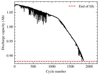
Figure 1: Capacity fade data points of a sample cell [b1c0] in the Toyota Research Institute dataset.

To formulate an approximation of the curvature we introduce the following two assumptions:

Assumption 1

A knee on the capacity fade curve of a lithium-ion cell has occurred before the end of the experiment.

Assumption 2

The $x$-values are evenly spaced. If not, the data points are fitted to a spline function and interpolated to become so.

We summarize our proposed curvature approximation in a step-by-step manner as follows:

1. To have our capacity knee identification algorithm as little affected as possible by variations in battery capacity magnitude, the raw capacity data points $\{x_{i},y_{i}\}_{i=1}^{N}$ are first normalized with the battery’s initial nominal capacity $Q_{nom}$. The resulting set of normalized data points is $\{x_{{n}_{i}},y_{{n}_{i}}\}_{i=1}^{N}$ where

   $$x_{{n}_{i}} =x_{i},$$

   $$y_{{n}_{i}} =\frac{y_{i}}{Q_{nom}}.$$

2. As a low-pass filter that utilizes the local least-square polynomial approximation, the Savitzky-Golay filter provides competitive denoising performance [29]. Additionally, it is more computationally efficient than other smoothing techniques with the potential for real-time applications. Therefore it is used to smooth the normalized data points $\{x_{{n}_{i}},y_{{n}_{i}}\}_{i=1}^{N}$. The resulting set of smoothed data points $\{x_{{sn}_{i}},y_{{sn}_{i}}\}_{i=1}^{N}$ is then used in the next step.

3. We approximate the curvature at data points $\{x_{{sn}_{i}},y_{{sn}_{i}}\}_{i=(ws+1)/2)}^{N-(ws-1)/2}$ by calculating their corresponding successive differences $y_{d_{i}}$ with a sliding window size $ws$ ($ws=3$ in this work), where

   $$x_{d_{i}} =x_{{sn}_{i}},$$

   $$y_{d_{i}} =y_{{sn}_{i-(ws-1)/2}}+y_{{sn}_{i+(ws-1)/2}}-2y_{{sn}_{i}}.$$

   With the assumption that the $x$-values are evenly spaced, then $y_{d_{i}}=0$ for any straight line. However, if any consecutive three points form a knee, then $y_{d_{i}}<0$ as the middle point $y_{{sn}_{i}}$ is now above the straight line that goes through the first point $y_{{sn}_{i-(ws-1)/2}}$ and the third point $y_{{sn}_{i+(ws-1)/2}}$. Analogously, if any consecutive three points form an elbow, then $y_{d_{i}}>0$.

The resulting approximated curvature of the example cell in Fig. 1 is illustrated in Fig. 2.

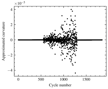
Figure 2: The approximated curvature of the sample cell [b1c0].

III-C Definitions

III-C1 Matrix Profile

Here, we first introduce all the necessary definitions related to a one-dimensional time series approximated curvature [30]:

Definition 1

A time series approximated curvature $\bm{Y}=\{y_{d_{1}},y_{d_{2}},...,y_{d_{M}}\}$ is an ordered sequence of real values that are evenly spaced, where $M=N-(ws-1)/2$.

Definition 2

A subsequence $\bm{Y}_{j,L}\subseteq\bm{Y}$ is a continuous subset of the values from $\bm{Y}$ of length $L$ starting from $j$, i.e., $\bm{Y}_{j,L}=\{y_{d_{j}},y_{d_{j+1}},...,y_{d_{j+L-1}}\}$, where $1\leq j\leq M-L+1$.

Definition 3

The set $\bm{Z}$ of a time series approximated curvature $\bm{Y}$ is an ordered set of all subsequences of $\bm{Y}$ obtained by sliding a window of length $L$ across $\bm{Y}$ such that: $\bm{Z}=\{\bm{Y}_{1,L},\bm{Y}_{2,L},...,\bm{Y}_{M-L+1,L}\}$, where $L$ is a user-defined subsequence length.

Definition 4

A self-similarity set $\bm{J}_{\bm{ZZ}}$ is a set containing pairs of each subsequence $\bm{Y}_{j,L}$ in $\bm{Z}$ with its nearest neighbor $\bm{Y}_{k,L}$ in $\bm{Z}$. We denote this as $\bm{J}_{\bm{ZZ}}=\{(\bm{Y}_{j,L},\bm{Y}_{k,L})\},j\neq k$.

Definition 5

A matrix profile $\bm{P}_{\bm{ZZ}}$ is a vector of the Euclidean distances between the two subsequences of each pair in $\bm{J}_{\bm{ZZ}}$.

Definition 6

A matrix profile index $\bm{I}_{\bm{ZZ}}$ of a self-similarity set $\bm{J}_{\bm{ZZ}}$ is a vector of integers where $\bm{I}_{\bm{ZZ}}[j]=k$ if $(\bm{Y}_{j,L},\bm{Y}_{k,L})\in\bm{J}_{\bm{ZZ}}$.

Given the definitions above, our main objective is to obtain two time-series, i.e., the matrix profile and the matrix profile index, to represent a time-series approximated curvature $\bm{Y}$ with the Euclidean distance and location of all its subsequences nearest neighbors to itself. From prior literature [30], it is known that these two time-series explicitly or implicitly contain the answers to many time-series data mining tasks. The algorithm that we adopt in this work to compute these two time-series is called Scalable Time series Anytime Matrix Profile (STAMP) [30]. STAMP is a time-series all-pairs one-nearest-neighbor search algorithm that uses the Fast Fourier Transform for speed and scalability. There are only two input parameters, i.e., the time series approximated curvature $\bm{Y}$, and a subsequence length $L$, where $L$ is the desired length of the time series pattern to search for.

III-C2 Arc Curve

Definition 7

An arc is an entry pair $(j,k)$ drawn from the $j$-th entry in the matrix profile index $\bm{I}_{\bm{ZZ}}$ to its nearest neighbor location at index $k$.

Definition 8

The Arc Curve (AC) for a time series approximated curvature $\bm{Y}$ of length $M$ is itself a time series of length $M$ containing nonnegative integer values. The $j$-th index in the AC specifies the number of arcs from the matrix profile index that cross over the location $j$.

Definition 9

A battery cell health degradation process with knee occurrence on the capacity fade curve consists of three discrete states $\bm{S}=[s_{1},s_{2},s_{3}]$ separated by two boundaries $\bm{B}=[b_{1},b_{2}]$. Here, $s_{1}$ represents the cell degradation process from the beginning of life till the knee-onset point, $s_{2}$ represents the cell degradation process from the knee-onset point to the knee point, and $s_{3}$ represents the cell degradation process from the knee point to the end of life.

With the advantage of having only two input parameters, i.e., the subsequence length $L$, and the number of states $N_{S}$, we adopt the regime extracting algorithm (REA) proposed by Gharghabi et al. [16] to extract the locations of the state changes from the AC, i.e., $\bm{B}=[b_{1},b_{2}]$. A pseudocode representation of the REA is given in Algorithm 1. To avoid returning the trivial minimum around the lowest point, REA does not return the locations of $N_{S}$ minimum values from the AC. Instead, once REA obtains a minimum value at a location, it sets an exclusion zone around the location as five times the subsequence length $L$. With the exclusion zone in place, REA repeats the search process as described above until all $N_{S}$ boundaries are found.

Algorithm 1 Regime Extracting Algorithm

1:Input: 1. AC: arc curve for approximated curvature

2:Input: 2. $L$: length of the subsequence

3:Input: 3. $N_{S}$: number of state changes

4:Initialize an empty array $\bm{A}$ of length $N_{S}$

5:for i=1:$N_{S}$ do

6:     $\bm{A}(i)=\mathrm{index}(\mathrm{min}(\mathrm{AC}))$

7:     Set an exclusion zone as five times the subsequence length $L$ before and after $\bm{A}(i)$

8:end for

9:Output: $\bm{A}$

In Fig. 3, the time series approximated curvature of the sample cell [b1c0] is shown at the top, while its corresponding AC is shown at the bottom. It can be seen from Fig. 3 that the approximated curvature is approximately equal to zero from the beginning of life till the first state change point $b_{1}$, which is identified as the capacity knee-onset using REA. Until the second state change point $b_{2}$, the approximated curvature fluctuates significantly, which indicates that the rate of change of degradation rate on the capacity fade curve fluctuates. After the second state change point $b_{2}$ that is identified as the capacity knee using REA, the degradation rate accelerates on the capacity fade curve till the end of life, as shown in Fig. 4.

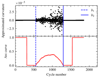
Figure 3: The time series approximated curvature (top) and corresponding arc curve (bottom) of the sample cell [b1c0].

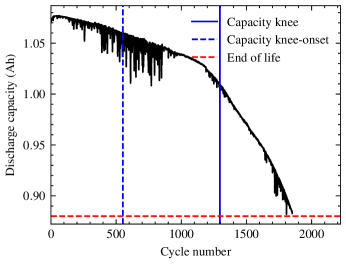
Figure 4: Identified capacity knee and capacity knee-onset of the sample cell [b1c0].

Now we can state the intuition of the time series segmentation algorithm using its corresponding AC in the context of a battery cell health degradation process. Suppose the time series approximated curvature $\bm{Y}$ of the sample cell [b1c0] has a state change at location $a$, we would expect very few arcs to cross over $a$ as most of the subsequences $\bm{Y}_{j,L}$ will find their nearest neighbors within the same state. Therefore, the height of the AC should be the lowest at the location of the boundary where the battery cell degradation process changes from one state to another.

IV Results and Discussion

IV-A Capacity Knee Identification on Experimental Dataset

As a fundamental step prior to addressing capacity knee-related battery problems, one would like to accurately identify knee-onset and knee on the capacity fade curve and then investigate the empirical relationship between knee-onset and end of life (80% of initial nominal capacity), and between knee and end of life. In this work, we first validate our proposed capacity knee identification algorithm using two experimental degradation datasets of two battery chemistry types (LFP and NMC). In addition, we also benchmark our capacity knee identification algorithm to the state-of-the-art knee identification algorithm in the literature, i.e., the double Bacon-Watts model [15].

With in total 169 LFP cells in the Toyota Research Institute dataset, capacity knee-onset and capacity knee were identified for each cell using the proposed capacity knee identification algorithm. For these, we found strong linear correlations between both knee-onset and end of life ($\rho=0.985$), and between knee and end of life ($\rho=0.993$), as shown in Fig. 5. These two strong linear correlations are further confirmed by the consistent identification results using the state-of-the-art knee identification algorithm in the literature, i.e., the double Bacon-Watts model. Apart from the strong correlations, by referring to the diagonal line [solid black line] in Fig. 5, it can be concluded that almost all the cells have knees occurring before the end of life. Moreover, the capacity knee algorithm identified both earlier knees and earlier knee-onsets than those identified using the double Bacon-Watts model.

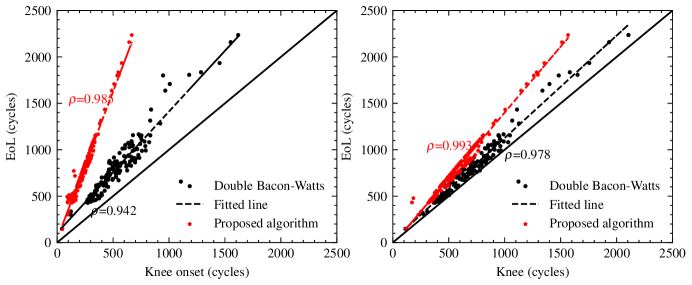
Figure 5: The relationship between knee-onset and end of life (left), knee and end of life (right) for 169 cells in the Toyota Research Institute dataset.

With the additional 22 NMC cells in the Sandia National Lab dataset, we again found strong linear correlations between knee-onset and end of life ($\rho=0.771$), and between knee and end of life ($\rho=0.792$) using the proposed capacity knee identification algorithm, as shown in Fig. 6. Interestingly, by referring to the diagonal line [solid black line] in Fig. 6, it can be concluded that there are NMC cells in the Sandia National Lab dataset that have knees occurring both before and after the end of life, which motivates the need for classifying retired batteries based on whether or not the knee has occurred in their first lives. In contrast, neither the knee-onset nor the knee identified using the double Bacon-Watts model shows strong correlations with the end of life, as shown in Fig. 6. In order to illustrate the possible cause of the weak correlations between both knee-onsets and knees, identified using the double Bacon-Watts model and end of life, we compared the knee-onsets and the knees obtained using the double Bacon-Watts model and the proposed capacity knee identification algorithm, respectively for a sample NMC cell [No.10] in the Sandia National Lab dataset. As illustrated in Fig. 7, the sample cell exhibits nonlinear capacity fade instead of linear capacity fade in the first degradation stage. The double Bacon-Watts model failed to identify both knee and knee-onset [green lines] while the proposed capacity knee identification algorithm successfully identified both knee and knee-onset [blue lines] on this NMC cell. As a matter of fact, almost all the NMC cells from the Sandia National Lab dataset exhibit nonlinear capacity fade instead of linear capacity fade in the first degradation stage, unlike the LFP cells in the Toyota Research Institute dataset.

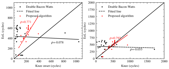
Figure 6: The relationship between knee-onset and end of life (left), and knee and end of life (right) for the Sandia National Lab dataset.

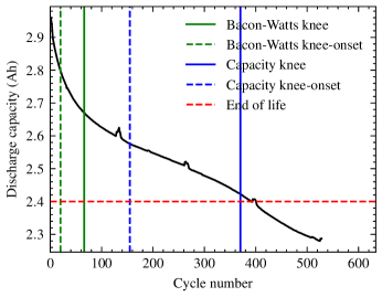
Figure 7: Knee-onset and knee obtained with the double Bacon-Watts model and proposed capacity knee identification algorithm of a sample cell [No.10] in the Sandia National Lab dataset.

The inconsistent results of using the double Bacon-Watts model to identify knee-onset and knee on two experimental battery degradation datasets indicate a lack of generalizability of the double Bacon-Watts model towards various battery chemistries for a wide range of operating conditions. In contrast, the generalizability of our proposed capacity knee identification algorithm has been demonstrated on the two experimental degradation data of two battery chemistry types under a wide range of operating conditions. The knee-onset identified using our proposed capacity knee identification algorithm provides the physical interpretation as the state change point, i.e., the rate of change of degradation rate on the capacity fade curve starts to fluctuate significantly until reaching the next state change point, which is the knee. Compared to the knee alone, the knee-onset can give a much earlier warning of accelerated degradation, on average there are 335 cycles for LFP cells and 262 cycles for NMC cells between the knee-onset and the identified knee. Therefore, the knee-onset identified using the proposed capacity knee identification algorithm may have significant economic value for sorting and regrouping of retired electric vehicle batteries, battery replacement planning, and battery repurposing to second-life applications.

IV-B Capacity Knee Identification on Synthetic Dataset

As a measure of the rate of change of degradation rate, the approximated curvature together with its corresponding AC with respect to cycle number for the simulated LGM50 cell is plotted in Fig. 8. A significant fluctuation of the approximated curvature can be observed in the second state of which the boundaries [dashed lines] were successfully inferred by the proposed identification algorithm. With a state change at each boundary, very few arcs cross over the boundary as most of the approximated curvature subsequences should find their nearest neighbors within the same state. Therefore, the height of the AC should be the lowest at each boundary where the LGM50 cell degradation process changes from one state to another, as shown at the bottom of Fig. 8. The measured discharge capacity fade curves are shown in Fig. 9. It can be seen that the knee is observable after approximately 680 cycles, and is followed by a sudden failure at 980 cycles due to the fact that the porosity at the negative electrode-separator interface reached zero. Again, the proposed capacity knee algorithm identified both earlier knees and earlier knee-onsets than those identified using the double Bacon-Watts model.

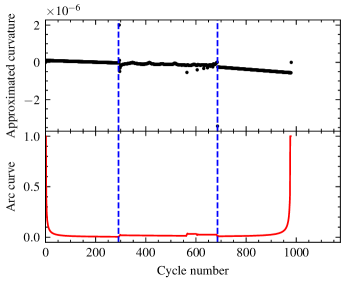
Figure 8: The time series approximated curvature (top) and corresponding arc curve (bottom) of the simulated cylindrical LGM50 cell.

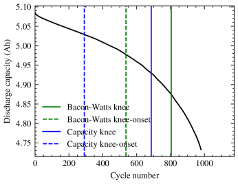
Figure 9: Comparison of knee-onset and knee obtained with the double Bacon-Watts model and proposed capacity knee identification algorithm of the cylindrical LGM50 cell.

The loss of capacity is solely caused by LLI due to SEI growth on the normal particle surface and on the crack surface. For large cracking rates, as is the case here, the LLI begins with a square root dependence on time until it reaches the inflection point, which is close to the identified capacity knee-onset point, as shown in Fig. 10. After the inflection point, the LLI accelerates exponentially as the cracks propagate. The accelerated LLI as the internal state change is the only cause for the simulated knee occurrence here.

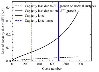
Figure 10: Capacity loss due to SEI growth on the normal particle surface and on the crack surface.

V Conclusion

Throughout the literature review, knees have been observed to occur within a window of 70-95 % of the initial nominal capacity in experimental testing of commercial lithium-ion cells of various chemistries and different operating conditions, which indicates the beginning of accelerated degradation and possible safety issues. To prepare for a successful second-life battery market, concerns arising from possible knee occurrence during first-life and second-life need to be addressed at the repurposing stage.

As the first step to address the aforementioned concerns, this paper proposes a robust capacity knee identification algorithm in order to identify capacity knee and capacity knee-onset on the capacity fade curve. Briefly, the approximated curvature was first used to represent the rate of change of capacity fade in discrete time, and then the capacity knee-onset and capacity knee were identified as the start and the end point, respectively, of a second discrete state in the whole degradation process. It was found that the approximated curvature fluctuated significantly in this second state. The proposed capacity knee identification algorithm was benchmarked to the state-of-the-art knee identification algorithm (i.e., the double Bacon-Watts model) on both synthetic degradation data and experimental degradation data of both LFP and NMC cells. In the results for the NMC cells, it was demonstrated that the state-of-the-art algorithm failed to identify the knee on the capacity fade curve while our proposed capacity knee identification algorithm successfully identified the knee. The results of capacity knee identification on synthetic degradation data provide some further physical interpretation of our proposed algorithm. Our proposed capacity knee identification algorithm can contribute to a successful second-life battery market from several aspects. In contrast to capacity knee identification alone, the knee-onset can give a much earlier warning of accelerated degradation (an average of 335 cycles was found for the LFP cells and an average of 262 cycles for the NMC cells between the knee-onset and the knee). Thus, the knee-onset identified using our proposed capacity knee identification algorithm can have significant economic value in early battery classification, early battery replacement planning, and even early battery repurposing to second-life applications; the capacity knee-onsets and capacity knees that are identified can also be used to systematically evaluate the knee-related prediction performance of both model-based methods and data-driven methods.

In an electric vehicle, we may not have access to all the cells, but at least the cell with the lowest capacity is accessible, and therefore it would be recommended to validate our proposed capacity knee identification algorithm on capacity fade data at pack level in the next step. Our proposed capacity knee identification algorithm has been validated only on battery degradation data from static cycling tests. Battery degradation data from dynamic cycling tests under realistic driving profiles are also suggested to be investigated. Historically, lithium plating has been considered the most common pathway for knee occurrence on the capacity fade curve, which will be studied for the validation purpose of our proposed algorithm in future work. Lastly, considering the close relationship between capacity knees and resistance/impedance elbows, it would also be interesting to adapt the proposed capacity knee identification algorithm accordingly so that the internal resistance elbows can be identified and predicted from internal resistance/impedance data.

References

- [1] R. Schmuch, R. Wagner, G. Hörpel, T. Placke, and M. Winter, “Performance and cost of materials for lithium-based rechargeable automotive batteries,” Nature Energy, vol. 3, no. 4, pp. 267–278, 2018.
- [2] E. Martinez-Laserna, E. Sarasketa-Zabala, I. V. Sarria, D.-I. Stroe, M. Swierczynski, A. Warnecke, J.-M. Timmermans, S. Goutam, N. Omar, and P. Rodriguez, “Technical viability of battery second life: A study from the ageing perspective,” IEEE Transactions on Industry Applications, vol. 54, no. 3, pp. 2703–2713, 2018.
- [3] M. Dubarry, C. Truchot, and B. Y. Liaw, “Synthesize battery degradation modes via a diagnostic and prognostic model,” Journal of power sources, vol. 219, pp. 204–216, 2012.
- [4] W. He, N. Williard, M. Osterman, and M. Pecht, “Prognostics of lithium-ion batteries based on dempster–shafer theory and the bayesian monte carlo method,” Journal of Power Sources, vol. 196, no. 23, pp. 10 314–10 321, 2011.
- [5] F. Yang, D. Wang, Y. Xing, and K.-L. Tsui, “Prognostics of li (nimnco) o2-based lithium-ion batteries using a novel battery degradation model,” Microelectronics Reliability, vol. 70, pp. 70–78, 2017.
- [6] P. M. Attia, A. Bills, F. B. Planella, P. Dechent, G. Dos Reis, M. Dubarry, P. Gasper, R. Gilchrist, S. Greenbank, D. Howey et al., ““knees” in lithium-ion battery aging trajectories,” Journal of The Electrochemical Society, vol. 169, no. 6, p. 060517, 2022.
- [7] E. Martinez-Laserna, E. Sarasketa-Zabala, D.-I. Stroe, M. Swierczynski, A. Warnecke, J.-M. Timmermans, S. Goutam, and P. Rodriguez, “Evaluation of lithium-ion battery second life performance and degradation,” in 2016 IEEE Energy Conversion Congress and Exposition (ECCE). IEEE, 2016, pp. 1–7.
- [8] C. Zhang, Y. Wang, Y. Gao, F. Wang, B. Mu, and W. Zhang, “Accelerated fading recognition for lithium-ion batteries with nickel-cobalt-manganese cathode using quantile regression method,” Applied Energy, vol. 256, p. 113841, 2019.
- [9] E. Wood, M. Alexander, and T. H. Bradley, “Investigation of battery end-of-life conditions for plug-in hybrid electric vehicles,” Journal of Power Sources, vol. 196, no. 11, pp. 5147–5154, 2011.
- [10] M. Arrinda, M. Oyarbide, H. Macicior, E. Muxika, H. Popp, M. Jahn, B. Ganev, and I. Cendoya, “Application dependent end-of-life threshold definition methodology for batteries in electric vehicles,” Batteries, vol. 7, no. 1, p. 12, 2021.
- [11] M. Baumann, L. Wildfeuer, S. Rohr, and M. Lienkamp, “Parameter variations within li-ion battery packs–theoretical investigations and experimental quantification,” Journal of Energy Storage, vol. 18, pp. 295–307, 2018.
- [12] L. Ahmadi, S. B. Young, M. Fowler, R. A. Fraser, and M. A. Achachlouei, “A cascaded life cycle: reuse of electric vehicle lithium-ion battery packs in energy storage systems,” The International Journal of Life Cycle Assessment, vol. 22, no. 1, pp. 111–124, 2017.
- [13] V. Satopaa, J. Albrecht, D. Irwin, and B. Raghavan, “Finding a” kneedle” in a haystack: Detecting knee points in system behavior,” in 2011 31st international conference on distributed computing systems workshops. IEEE, 2011, pp. 166–171.
- [14] W. Diao, S. Saxena, B. Han, and M. Pecht, “Algorithm to determine the knee point on capacity fade curves of lithium-ion cells,” Energies, vol. 12, no. 15, p. 2910, 2019.
- [15] P. Fermín-Cueto, E. McTurk, M. Allerhand, E. Medina-Lopez, M. F. Anjos, J. Sylvester, and G. Dos Reis, “Identification and machine learning prediction of knee-point and knee-onset in capacity degradation curves of lithium-ion cells,” Energy and AI, vol. 1, p. 100006, 2020.
- [16] S. Gharghabi, Y. Ding, C.-C. M. Yeh, K. Kamgar, L. Ulanova, and E. Keogh, “Matrix profile viii: domain agnostic online semantic segmentation at superhuman performance levels,” in 2017 IEEE international conference on data mining (ICDM). IEEE, 2017, pp. 117–126.
- [17] K. A. Severson, P. M. Attia, N. Jin, N. Perkins, B. Jiang, Z. Yang, M. H. Chen, M. Aykol, P. K. Herring, D. Fraggedakis et al., “Data-driven prediction of battery cycle life before capacity degradation,” Nature Energy, vol. 4, no. 5, pp. 383–391, 2019.
- [18] P. M. Attia, A. Grover, N. Jin, K. A. Severson, T. M. Markov, Y.-H. Liao, M. H. Chen, B. Cheong, N. Perkins, Z. Yang et al., “Closed-loop optimization of fast-charging protocols for batteries with machine learning,” Nature, vol. 578, no. 7795, pp. 397–402, 2020.
- [19] Y. Preger, H. M. Barkholtz, A. Fresquez, D. L. Campbell, B. W. Juba, J. Romàn-Kustas, S. R. Ferreira, and B. Chalamala, “Degradation of commercial lithium-ion cells as a function of chemistry and cycling conditions,” Journal of The Electrochemical Society, vol. 167, no. 12, p. 120532, 2020.
- [20] S. G. Marquis, V. Sulzer, R. Timms, C. P. Please, and S. J. Chapman, “An asymptotic derivation of a single particle model with electrolyte,” Journal of The Electrochemical Society, vol. 166, no. 15, p. A3693, 2019.
- [21] V. Sulzer, S. G. Marquis, R. Timms, M. Robinson, and S. J. Chapman, “Python battery mathematical modelling (pybamm),” Journal of Open Research Software, vol. 9, no. 1, 2021.
- [22] F. Single, A. Latz, and B. Horstmann, “Identifying the mechanism of continued growth of the solid–electrolyte interphase,” ChemSusChem, vol. 11, no. 12, pp. 1950–1955, 2018.
- [23] C. R. Birkl, M. R. Roberts, E. McTurk, P. G. Bruce, and D. A. Howey, “Degradation diagnostics for lithium ion cells,” Journal of Power Sources, vol. 341, pp. 373–386, 2017.
- [24] J. Christensen and J. Newman, “Stress generation and fracture in lithium insertion materials,” Journal of Solid State Electrochemistry, vol. 10, no. 5, pp. 293–319, 2006.
- [25] R. Deshpande, M. Verbrugge, Y.-T. Cheng, J. Wang, and P. Liu, “Battery cycle life prediction with coupled chemical degradation and fatigue mechanics,” Journal of the Electrochemical Society, vol. 159, no. 10, p. A1730, 2012.
- [26] S. E. O’Kane, W. Ai, G. Madabattula, D. Alonso-Alvarez, R. Timms, V. Sulzer, J. S. Edge, B. Wu, G. J. Offer, and M. Marinescu, “Lithium-ion battery degradation: how to model it,” Physical Chemistry Chemical Physics, vol. 24, no. 13, pp. 7909–7922, 2022.
- [27] T. Raj, A. A. Wang, C. W. Monroe, and D. A. Howey, “Investigation of path-dependent degradation in lithium-ion batteries,” Batteries & Supercaps, vol. 3, no. 12, pp. 1377–1385, 2020.
- [28] T. C. Bach, S. F. Schuster, E. Fleder, J. Müller, M. J. Brand, H. Lorrmann, A. Jossen, and G. Sextl, “Nonlinear aging of cylindrical lithium-ion cells linked to heterogeneous compression,” Journal of Energy Storage, vol. 5, pp. 212–223, 2016.
- [29] A. Savitzky and M. J. Golay, “Smoothing and differentiation of data by simplified least squares procedures.” Analytical chemistry, vol. 36, no. 8, pp. 1627–1639, 1964.
- [30] C.-C. M. Yeh, Y. Zhu, L. Ulanova, N. Begum, Y. Ding, H. A. Dau, D. F. Silva, A. Mueen, and E. Keogh, “Matrix profile i: all pairs similarity joins for time series: a unifying view that includes motifs, discords and shapelets,” in 2016 IEEE 16th international conference on data mining (ICDM). Ieee, 2016, pp. 1317–1322.