Evading DeepFake Detectors via Adversarial Statistical Consistency

Abstract

In recent years, as various realistic face forgery techniques known as DeepFake improves by leaps and bounds, more and more DeepFake detection techniques have been proposed. These methods typically rely on detecting statistical differences between natural (i.e., real) and DeepFake-generated images in both spatial and frequency domains. In this work, we propose to explicitly minimize the statistical differences to evade state-of-the-art DeepFake detectors. To this end, we propose a statistical consistency attack (StatAttack) against DeepFake detectors, which contains two main parts. First, we select several statistical-sensitive natural degradations (i.e., exposure, blur, and noise) and add them to the fake images in an adversarial way. Second, we find that the statistical differences between natural and DeepFake images are positively associated with the distribution shifting between the two kinds of images, and we propose to use a distribution-aware loss to guide the optimization of different degradations. As a result, the feature distributions of generated adversarial examples is close to the natural images. Furthermore, we extend the StatAttack to a more powerful version, MStatAttack, where we extend the single-layer degradation to multi-layer degradations sequentially and use the loss to tune the combination weights jointly. Comprehensive experimental results on four spatial-based detectors and two frequency-based detectors with four datasets demonstrate the effectiveness of our proposed attack method in both white-box and black-box settings.

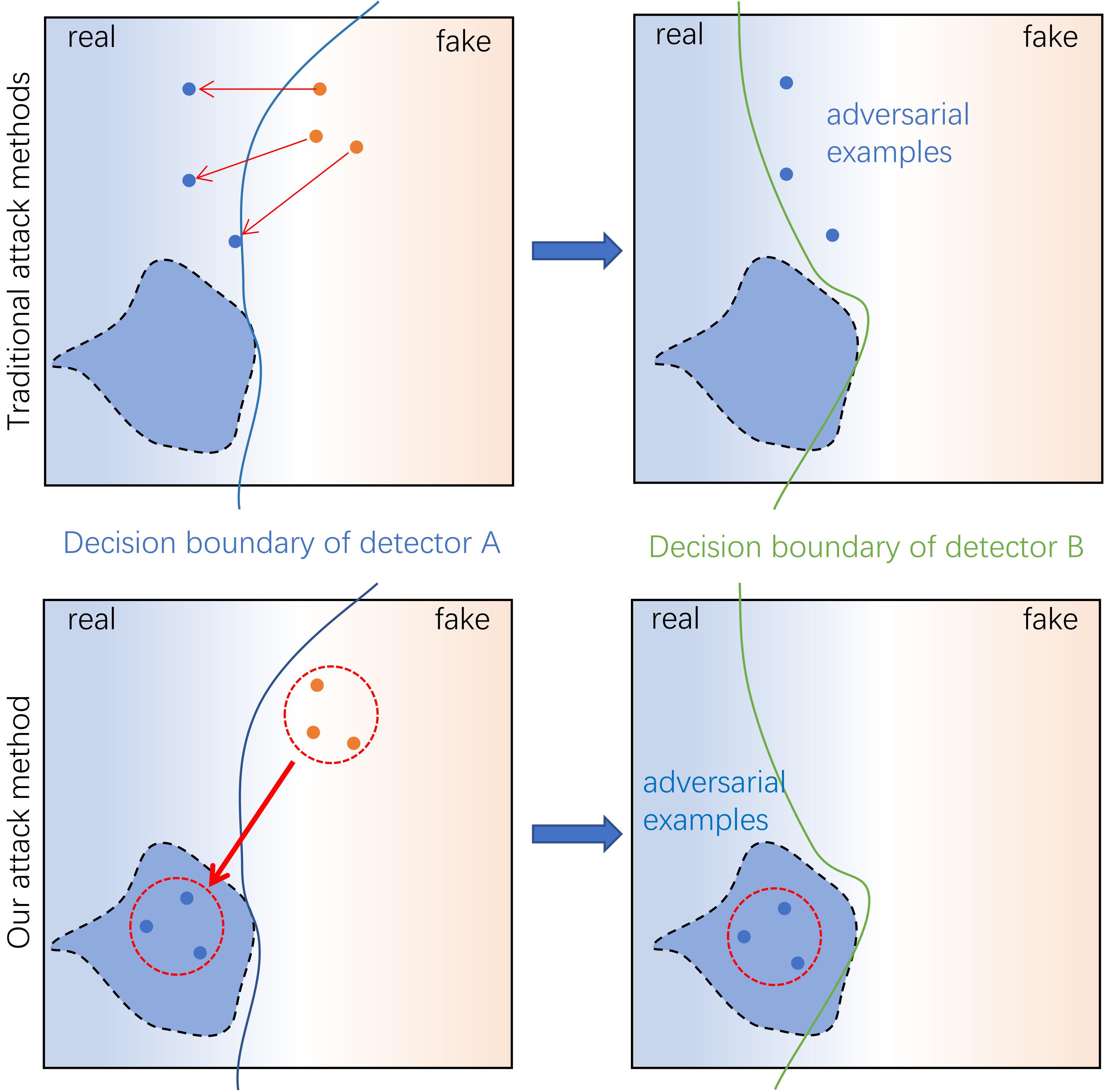
Figure 1: Principle of our method. The light blue region and the light red region represent the embedding space of natural/real images and fake images, respectively. The dark blue region represents the embedding spaces of real images shared by different detectors. The first row shows that a typical attack can map the fake samples (i.e., the orange points) to the ‘real’ samples that can fool detector A but fail to mislead detector B. The second row shows that our method is to map the fake samples to the common regions of different detectors, which can fool both detectors.

1 Introduction

Recent advances in facial generation and manipulation using deep generative approaches (i.e., DeepFake [30]) have attracted considerable media and public attentions. Fake images can be easily created using a variety of free and open-source tools. However, the misuse of DeepFake raises security and privacy concerns, particularly in areas such as politics and pornography [6, 46]. The majority of back-end technologies for DeepFake rely on generative adversarial networks (GANs). As GANs continue to advance, state-of-the-art (SOTA) DeepFake has achieved a level of sophistication that is virtually indistinguishable to human eyes.

Although these realistic fake images can spoof human eyes, SOTA DeepFake detectors can still effectively detect subtle ‘fake features’ by leveraging the powerful feature extraction capabilities of deep neural networks (DNNs). However, recent studies [11, 2] have shown that these detectors are vulnerable to adversarial attacks that can bypass detectors by injecting perturbations into fake images. Additionally, adversarial examples pose a practical threat to DeepFake detection if they can be transferred between different detectors. Adversarial attacks are often used to verify the robustness of DeepFake detectors [25]. Therefore, in order to further research and develop robust DeepFake detectors, it is crucial to develop effective and transferable adversarial attacks.

Several previous studies have explored the transferability of adversarial examples [51, 50], which refers to the ability of adversarial examples designed for a specific victim model to attack other models trained for the same task. However, achieving transferable attacks against DeepFake detectors is particularly challenging due to variations in network architectures and training examples caused by different data augmentation and pre-processing methods. These differences often result in poor transferability of adversarial examples crafted from typical attack methods when faced with different DeepFake detectors.

Current detection methods typically rely on detecting statistical differences in spatial and frequency domains between natural and DeepFake-generated images, (as explained in Section 3), and various detectors share some common statistical properties of natural images [36, 8, 53]. These prior knowledge and discoveries inspire us to design an attack method with strong transferability that can minimize statistical differences explicitly. Toward the transferable attack, we propose a novel attack method, StatAttack. Specifically, we select three types of statistical-sensitive natural degradations, including exposure, blur, and noise, and add them to fake images in an adversarial manner. In addition, our analysis indicates that the statistical differences between the real and fake image sets are positively associated with their distribution shifting. Hence, we propose to mitigate these differences by minimizing the distance between the feature distributions of fake images and that of natural images. To achieve this, we introduce a novel distribution-aware loss function that effectively minimizes the statistical differences. Figure 1 illustrates the principle of our proposed attack method. Moreover, We expand our attack method to a more powerful version, MStatAttack. This improved approach performs multi-layer degradations and can dynamically adjust the weights of each degradation in different layers during each attack step. With the MStatAttack, we can develop more effective attack strategies and generate adversarial examples that appear more natural.

Our contributions can be summarized as the following:

• We propose a novel natural degradation-based attack method, StatAttack. StatAttack can fill the feature distributions difference between real and fake images by minimizing a distribution-aware loss.

• To enhance the StatAttack, we further propose a multi-layer counterpart, MStatAttack, which can select a more effective combination of perturbations and generate more natural-looking adversarial examples.

• We conduct comprehensive experiments on four spatial-based and two frequency-based DeepFake detectors using four datasets. The experimental results demonstrate the effectiveness of our attack in both white-box and black-box settings.

2 Related Work

DeepFake generation. Generative adversarial networks (GANs) and their variants have achieved impressive results in image generation and manipulation, leading to the development of DeepFake technology. DeepFake utilizes GANs to generate various types of fake images or videos. The current DeepFake techniques can be roughly categorized into three categories: entire face synthesis [40, 31, 32], face identity swap [12, 39], and face manipulation [34, 21, 14].

Entire face synthesis aims to generate realistic human faces that do not really exist, such as ProGAN [31] and StyleGAN [32] developed by NVIDIA. The face identity swap replaces a person’s face with the face of the target person. FaceApp and FaceSwap are two Popular DeepFake generation tools that employ GANs to achieve identity swapping. In face manipulation, StarGAN [5], STGAN [34], A3GAN [52], and AttGAN [21] are employed to edit and manipulate the attributes and expressions of human faces, such as changing the hair color, adding beards, wearing glasses or creating smiling faces.

Malicious applications that utilize these generation methods may pose a significant threat to public information security. In order to fully evaluate the effectiveness of our attack, we conduct a comprehensive evaluation based on the generation methods described above. The generated face dataset includes entire face synthesis images, face identity swap images, and face manipulation images, allowing for a comprehensive analysis of the attack’s performance.

DeepFake detection. To prevent the misuse of DeepFake technologies, several DNN-based DeepFake detection methods have been proposed. DeepFake detection is essentially a binary classification problem that involves distinguishing between fake images and natural images. Among the existing detection methods, some works are focused on extracting the spatial domain information [24, 48, 27, 41] of images for DeepFake detection, while others explore the difference in frequency domain information [10, 42, 1] between fake images and natural images. These detection methods are entirely data-driven and aim to enable the model to learn the statistical differences between fake and natural images. With the powerful feature extraction capability of DNNs, these detection methods achieve superior detection results under their respective experimental settings. To fully evaluate the effectiveness of our attack method, we perform attack experiments on both spatial and frequency-based detectors to evaluate the effectiveness of our attacks.

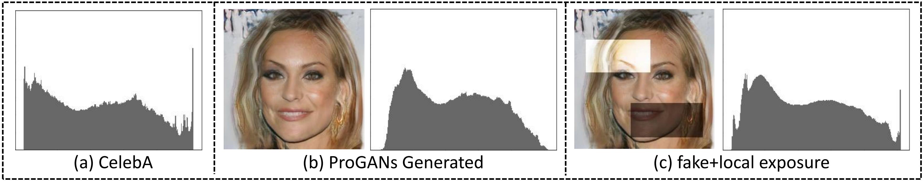
Figure 2: Brightness statistic differences. (a) shows the average brightness histogram of a natural face dataset, while (b) shows the average brightness histogram of a ProGAN-generated fake face dataset that lacks saturated and under-exposed region. (c) is the same datasets as (b) with partial exposure adjustment. After adjusting the local brightness, saturated and under-exposed pixel values in fake images histogram appear.

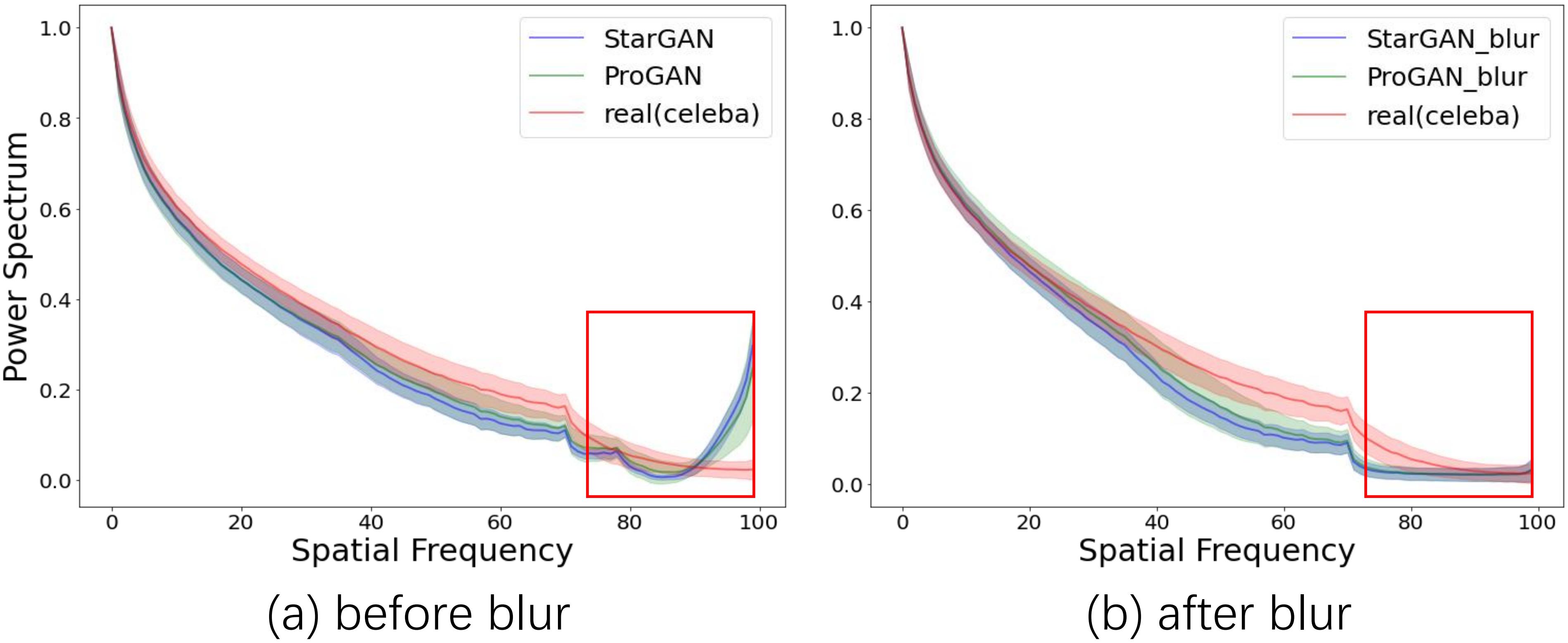
Figure 3: Frequency Statistical differences (power spectrum). (a) shows that GAN-generated images suffer from the dramatic increment of the high-frequency components compared with natural images. (b) reveals that the Gaussian blurring process can reduce these frequency differences.

Adversarial attack. Adversarial attack aims to generate adversarial perturbations and add them to inputs. The generated adversarial examples can fool the target model into predicting an incorrect label. Some works investigate the effect of additive perturbations on classifier robustness in a white-box setting [15, 35, 3], while others focus on studying the transferability of the adversarial example on the same task in a black-box setting [26, 4, 18, 44]. More recently, some other works have tried to employ natural degradation as attack perturbations, such as motion blur, vignetting, rain streaks, exposure, and watermark [13, 19, 47, 29].

For adversarial attacks against DeepFake detection, several existing works have studied the robustness of DeepFake detectors with additive perturbation-based attacks in different experimental settings [38, 11, 33, 25, 28]. Meanwhile, some works point out that adversarial examples with strong transferability can pose a practical threat to DeepFake detection [38, 2]. To achieve transferable attacks, we investigate the potential of natural degradation-based attacks to evade various DeepFake detectors.

3 Statistical Differences

Several detection methods reveal statistical differences between natural and fake images in both the frequency and spatial domains. As seen in Figure 2, McCloskey et al. [36] demonstrate that the network architecture and training process of GANs can cause differences in the brightness statistics between GAN-generated images and natural images. For example, some GANs are only capable of generating images with limited intensity values and fail to produce saturated and under-exposed regions. In addition, as illustrated in Figure 3, Durall et al. [8] explore the statistical differences in frequency information between natural and GAN-generated images, revealing significant differences in high-frequency components. Similarly, as we can see from Figure 4 (a), Zhang et al. [53] find some statistical clues by directly observing the spectrograms of GANs-generated images. Their experimental results show that the GANs would inevitably leave regular high-frequency artifacts in the manipulated images. To mitigate these differences, we aim to add corresponding adversarial degradations.

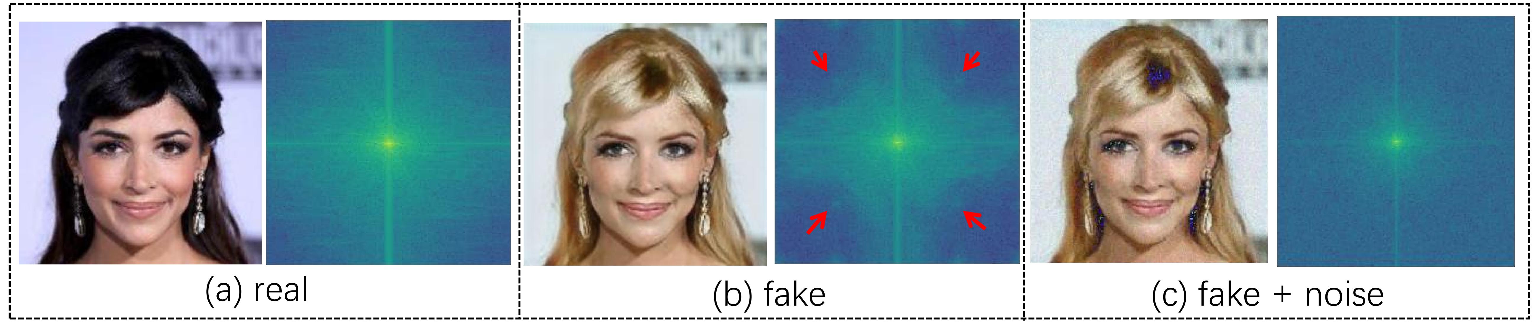
Figure 4: Frequency Statistical differences (spectrogram). (a) is a real face image, (b) is a stargan-tampered image (Black hair turns yellow), and (c) is a fake image with random noise added. Their histograms are shown on the right of each image (Zoom in to see details). Compared to the natural image, regular frequency artifacts appear in the spectrogram of the stargan-tampered image (indicated by a red arrow). After adding noise, the high-frequency artifacts in the fake image disappear.

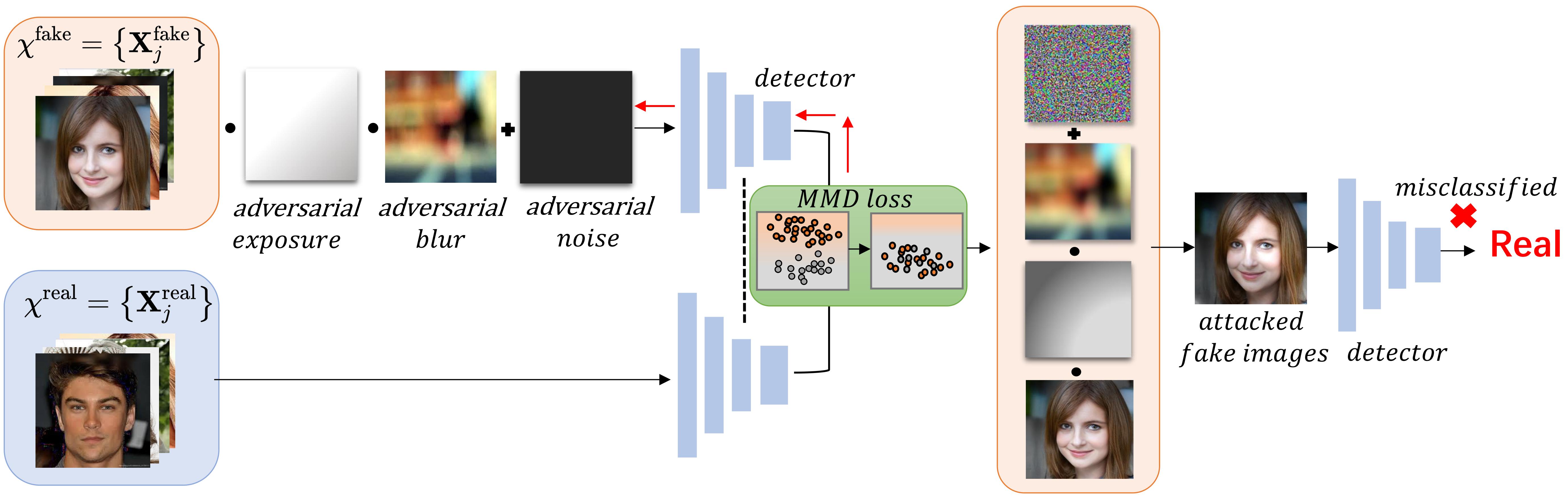
Figure 5: Pipeline of our attack. First, we add initialized adversarial degradations (adversarial exposure, adversarial blur, and adversarial noise) to the fake images. Then, We collect the feature distributions of both natural and fake images and calculate their MMD values. Finally, we optimize the perturbation parameters by minimizing the loss function and applying the optimized degradations to fake images.

4 Statistical Consistency Attack (StatAttack)

In this section, we first introduce three natural degradations that reduce the statistical differences between natural and fake images, which are referred to as statistical-sensitive degradations. We then demonstrate how to adversarially add these natural degradations to the fake images. Finally, we present our objective function and explain how it reduces statistical differences effectively.

4.1 Statistical-Sensitive Degradation

Selection of degradations. We discuss three common natural degradations that can effectively reduce the statistical differences in Section 3: ❶ Changing exposure. Adjusting the brightness values of pixels in local areas can change the brightness distribution of fake images. As shown in Figure 2 (c), oversaturating and underexposing the pixels in local areas of fake images can make their brightness distributions similar to those of natural images. ❷ Adding blur. Filtering out the high-frequency components in fake images with a Gaussian low-pass filter can reduce the statistical differences in the frequency domain. As illustrated in Figure 3, after performing Gaussian filtering on fake images, the distribution of high-frequency components becomes consistent with that of natural images. ❸ Adding noise. Figure 4 (c) shows the spectrum of fake images after adding random noise, and we see that the regular artifacts in fake images are eliminated. It is worth noting that adding local exposure to the image can change the information not only in the spatial domain but also in the frequency domain. Furthermore, Gaussian filtering can also reduce some regular high-frequency artifacts in the fake image. In the following, we introduce how to add the three degradations in an adversarial way.

Naturalness adversarial exposure. We aim to inject local exposure into the fake images, making their brightness statistics more similar to natural images. Besides, since natural-world exposure changes smoothly, the exposure injected into the fake image should also have similar properties ( i.e., adjacent pixels in an image have similar exposure values). In order to achieve both of these objectives, we adopt the adversarial exposure generation model proposed by Gao et al. [13]. This model comprises two main components: a polynomial model for generating exposure and a smoothing formula for maintaining the naturalness of the exposure. Let $\tilde{\mathbf{E}}$ represent the polynomial model for generating exposure, and $\mathbf{X}^{\text{fake}}$ represent a fake image. We can inject adversarial exposure into the fake image by

$$P_{e}(\mathbf{X}^{\text{fake}})=\text{log}^{-1}(\tilde{\mathbf{X}}^{\text{fake}}+\tilde{\mathbf{E}}),$$ (1)

where the operation ‘$\tilde{\cdot}$’ represents the logarithmic operation. The polynomial model comprises two sets of parameters, denoted by a and $\varphi$, which are optimized to generate the adversarial exposure. To maintain the naturalness of the exposure, we constrain the values of a and $\varphi$ by adding the smoothing equation to the loss function

$$S\left(\textbf{a},\varphi\right)=-\lambda_{a}\left\|\textbf{a}\right\|_{2}^{2}-\lambda_{\varphi}\left\|\bigtriangledown\varphi\right\|_{2}^{2},$$ (2)

where the hyper-parameters $\lambda_{a}$ and $\lambda_{\varphi}$ are used to regulate the balance between adversarial attack and smoothness.

Adversarial Gaussian blur. For a normal Gaussian blur, Gaussian kernels used at different locations in an image have the same value. To add Gaussian blur degradation in an adversarial way, we propose to design Gaussian kernels as learnable adversarial kernels. This approach allows the adversarial perturbations to be applied adaptively at different locations of the image [19]. Specifically, we denote $\sigma_{x_{i},y_{i}}$ as the initial standard deviation of the Gaussian kernel at each pixel position, where $i$ denotes the $i$-th pixel and $x_{i},y_{i}$ presents the corresponding image coordinates. We aim to learn a standard deviation map $\sigma$, where the $\sigma_{x_{i},y_{i}}$ represents the standard deviation at each pixel position. Note that, the larger $\sigma$ should result in more blurry images. With $\sigma_{x_{i},y_{i}}$, we calculate the adversarial Gaussian kernel for the $i$th pixel (i.e., $\mathbf{H}_{i}$) as follows:

$$\mathbf{H}_{i}(u,v)=\frac{1}{2\pi\left(\sigma_{x_{i},y_{i}}\right)^{2}}exp\left(-\frac{u^{2}+v^{2}}{2\pi\left(\sigma_{x_{i},y_{i}}\right)^{2}}\right),$$ (3)

where $u$ and $v$ represent the relative coordinate of the point within the Gaussian kernel to the central pixel $(x_{i},y_{i})$.With the adversarial Gaussian kernel, we blur the fake image by

$$P_{b}(\mathbf{X}^{\text{fake}})=\sum_{i\in\mathcal{N}(i)}g(\mathbf{X}_{i}^{\text{fake}},k)\ast\mathbf{H}_{i}.$$ (4)

In this equation, $\mathcal{N}(i)$ refers to all pixels in $\mathbf{X}_{fake}$, $g(\mathbf{X}_{i}^{\text{fake}},k)$ represents the region centered at the $i$th pixel and enclosed within a Gaussian kernel of radius $k$, and the term ‘$\ast$’ denotes the filtering operation. We can feed the generated image $P_{b}(\mathbf{X}^{\text{fake}})$ an adversarial-related loss function and minimize it to get $\{\sigma_{x_{i},y_{i}}\}$ and $\mathbf{H}_{i}$ via Eq. (4). Subsequently, we apply pixel-level Gaussian blur on the fake images through the computed Gaussian kernel.

Adversarial noise. To generate adversarial noise, we adopt a simple and effective method. The adversarial noise is denoted as follows:

$$P_{n}(\mathbf{X}^{\text{fake}})=\mathbf{X}^{\text{fake}}+\mathbf{N}_{a},$$ (5)

where $\mathbf{N}_{a}$ refers to an adversarial noise map with the same size as $\mathbf{X}^{\text{fake}}$. During each attack step, we generate the adversarial noise by minimizing our adversarial loss function and subsequently adding it to each fake image. To ensure that the adversarial noise does not significantly impact the quality of the image, we enforce sparsity on $\mathbf{N}_{a}$ using a constraint term. This constraint term is incorporated into the final objective function.

In StatAttack, we apply these three perturbations sequentially to fake images. Based on Eq. (1), (4), and (5), we can summarize the aforementioned perturbations as follows:

$$P_{\theta}(\mathbf{X}^{\text{fake}})=P_{n}(P_{b}(P_{e}(\mathbf{X}^{\text{fake}}))),$$ (6)

where the $P_{\theta}(\mathbf{X}^{\text{fake}})$ contains four sets of parameters to be optimized, i.e., $\left\{\textbf{a},\varphi,\sigma,\mathbf{N}_{a}\right\}$.

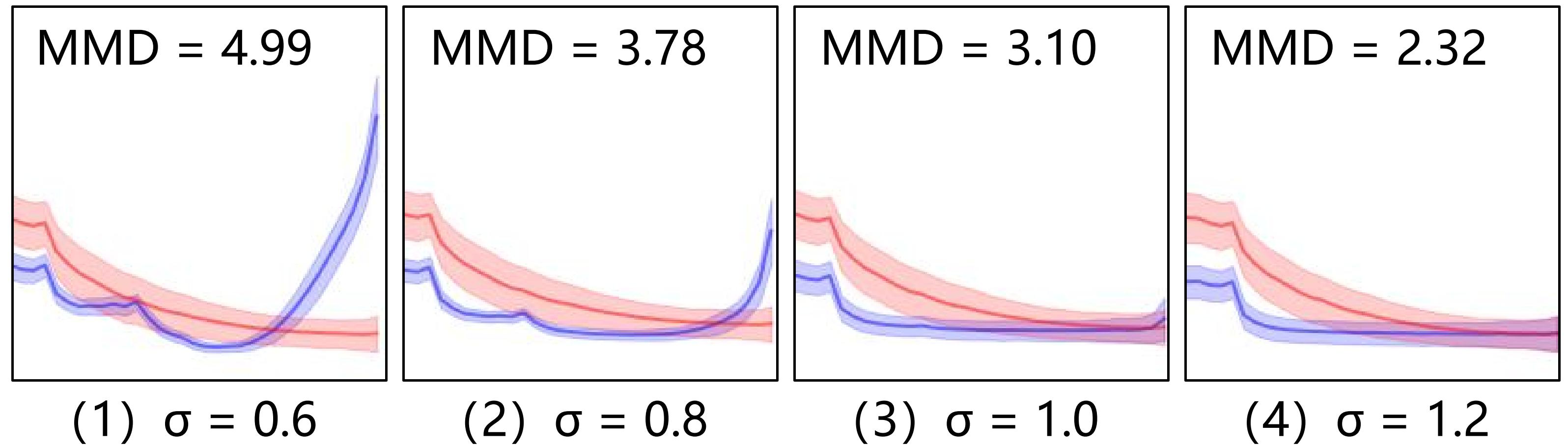
Figure 6: Correlations between statistical differences and the distribution shifting of the natural and fake image sets. (1) - (4) display the power spectrum and the MMD values between feature distributions of two sets. The blue curves represent the high-frequency components of GAN-generated images while the red curves depict natural ones. We process the fake images using Gaussian blur with various Gaussian kernels $\sigma$ and observe that as the high-frequency statistical differences decrease, the MMD values also decrease.

4.2 Distribution-aware Statistical Consistency

Given a set of real images and a set of fake images, we study correlations between statistical differences and distribution shifting of the two sets and find that statistical differences are positively associated with the distribution shifting between the two sets. Figure 6 illustrates a simple experiment that we investigate this relationship. In this experiment, we first collect a set of natural images and a set of StarGan-generated fake images, and use a Gaussian filter to handle fake images with varying $\sigma$. Then, we use maximum mean discrepancy (MMD) [17] to measure the distance between the feature distributions of the filtered fake images and natural images. It is worth noting that increasing the $\sigma$ can reduce the high-frequency spectrum in the fake images. We find that the MMD value decreases as the statistical difference reduces. Moreover, previous studies [49, 9] have pointed out that the MMD between two feature distributions at the $i$-th layer is end-to-end differentiable, enabling the use of MMD as a loss function.

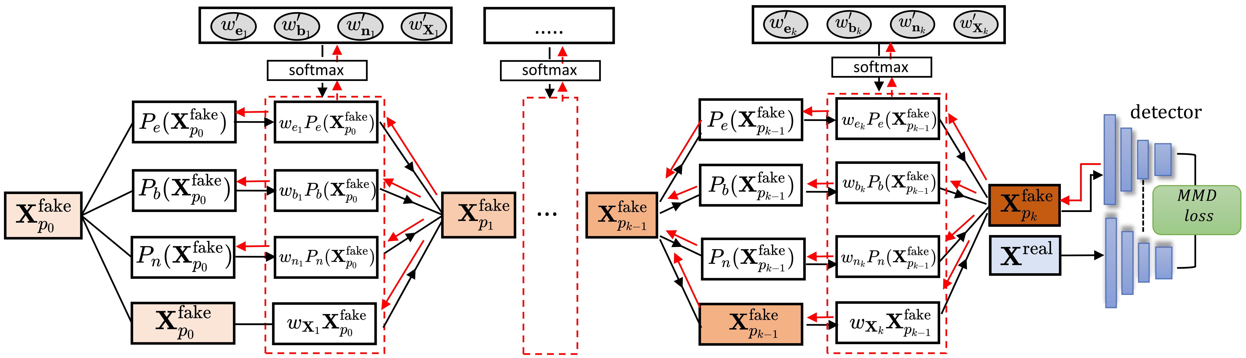
Figure 7: Architecture of MStatAttack. The weights and parameters of each attack pattern are optimized jointly when minimizing the objective function.

Objective function. An attack is considered successful for a binary classifier if the generated adversarial example is classified as the opposite class. Our objective is to generate adversarial examples that closely resemble natural images in terms of feature distributions. Let $\chi^{\text{fake}}=\left\{\mathbf{X}^{\text{fake}}_{j}\right\}$ and $\chi^{\text{real}}=\left\{\mathbf{X}^{\text{real}}_{j}\right\}$ represent a set of fake and natural images. We define our objective function as follows:

$$\begin{split}&\underset{\textbf{a},\varphi,\sigma,\mathbf{N}_{a}}{arg\min}J_{MMD}\left(P_{\theta}\left(\chi^{\text{fake}}\right),\chi^{\text{real}}\right)+S(\textbf{a},\varphi),\\ &\qquad\qquad\qquad\mathrm{subject\;to}\;\left\|\mathbf{N}_{a}\right\|_{p}\leq\epsilon\end{split}$$ (7)

where $J_{MMD}(\cdot)$ represents the MMD value between the two feature distributions in a certain detector layer. We calculate the parameters of adversarial exposure, blur, and noise by optimizing Eq. (7).

Algorithm. As shown in Figure 5. First, we initialize the parameters $\left\{\textbf{a},\varphi,\sigma,\mathbf{N}_{a}\right\}$ for the three perturbations and add them to the fake images. Next, we collect the feature distributions of both the natural and fake images on the global pooling layer in each DNN-based detector model and calculate their MMD values. To optimize the perturbation parameters, we use sign gradient descent to minimize Eq. (7). Finally, we apply the optimized values of $\left\{\textbf{a},\varphi,\sigma,\mathbf{N}_{a}\right\}$ to the raw fake images, resulting in the generation of adversarial fake images.

5 Multi-layer StatAttack (MStatAttack)

Repeatedly adding adversarial perturbations to an image may increase the success rate of attacks. Hence, we further extend the StatAttack to a more powerful version, i.e., MStatAttack, where we extend the single-layer degradation to multi-layer degradations sequentially and use the loss to tune the combination weights jointly.

Specifically, as depicted in Figure 7, MStatAttack employs multiple layers to process the input. At the $k$th layer, MStatAttack takes the output of the $(k-1)$th layer, which is denoted as $\mathbf{X}^{\text{fake}}_{p_{k-1}}$, and applies three types of adversarial degradation (i.e., exposure, blur, and noise) in parallel. Then, we maintain four weights (i.e., $w^{\prime}_{e_{k}}$, $w^{\prime}_{b_{k}}$, $w^{\prime}_{n_{k}}$, $w^{\prime}_{\mathbf{X}_{k}}$) to mix $\mathbf{X}^{\text{fake}}_{p_{k-1}}$ and its three perturbed versions, obtaining the output of the $k$th layer. To make sure the sum of the four weights equal one, we feed them to a softmax layer and get (i.e., $w_{e_{k}}$, $w_{b_{k}}$, $w_{n_{k}}$, $w_{\mathbf{X}_{k}}$ ). The perturbation of each layer can be written as

$$\begin{split}\mathbf{X}^{\text{fake}}_{p_{k}}&=w_{e_{k}}P_{e}(\mathbf{X}^{\text{fake}}_{p_{k-1}})+w_{b_{k}}P_{b}(\mathbf{X}^{\text{fake}}_{p_{k-1}})\\ &+w_{n_{k}}P_{k}(\mathbf{X}^{\text{fake}}_{p_{n-1}})+w_{\mathbf{X}_{k}}\mathbf{X}^{\text{fake}}_{p_{k-1}},\ n\geq 1\end{split}$$ (8)

where the $\mathbf{X}^{\text{fake}}_{p_{k}}$ represents the adversarial examples generated at $k$th layer. During optimization, the raw weights and all degradation parameters are jointly optimized based on the loss function. The softmax layer ensures that the updated weights add up to one, preventing intensity overflow during the image mixing process.

In addition to automatically selecting the appropriate attack strategy ( i.e., perturbation combinations ), MStatAttack can enhances the generated adversarial examples by incorporating more components from the raw fake images, resulting in visually closer raw fake images.

Table 1: Statistics of the collected dataset. The first column is the fake faces, the second column is the type of fake faces, the third column is the collection method, and the fourth column is the real data source for generating the fake faces.

Fake Data	Fake Type	Collection	Real Source
FF++	face identity swap	FaceForensics++	FaceForensics++
StyleGANv2	entire face syhthesis	self-synthesis	FFHQ
StarGAN	face manipulation	self-synthesis	CelebA
ProGAN	entire face syhthesis	self-synthesis	CelebA-HQ

6 Experiments

6.1 Experimental Setups

Dataset. We conduct experiments on four datasets to evaluate our method. For entire face synthesis, we use StyleGANv2 [32] and ProGAN [31] to generate high-quality fake face images. For face attribute manipulation, we employ StarGAN [5] to modify the attributes of natural face images, where the modified attributes are hair color, gender, and age. For face identity swap, we use the DeepFake dataset provided in the FaceForensics++ [43] benchmark, which was produced using the publicly available tool. Table 1 presents the statistics of our collected fake dataset. For real face images, we use real face images from CelebA, FFHQ, and FaceForensics++ dataset.

Victim detectors. For the spatial-based detectors, we use four spatial-based classification models, i.e., ResNet50 [20], EfficentNet-b4 [45], DenseNet[23], and MobileNet[22]. For the frequency-based detectors, we adopt two popular detectors, DCTA[10] and DFTD[53]. To ensure fair evaluations, we reproduce the PyTorch version of DCTA and rewrite the frequency domain transform operations involved in both methods as a network structure layer. Table 2 shows the accuracy of these detectors on each dataset.

Table 2: The accuracy of each detector on different datasets.

Model&  DataSet Model& DataSet	ResNet	EffNet	DenNet	MobNet	DCTA	DFTD
FF++	94.2%	93.8%	91.5%	94.4%	93.1%	91.6%
StyleGANv2	98.7%	97.5%	99.2%	97.2%	98.5%	97.4%
StarGAN	97.6%	98.9%	98.4%	96.4%	100%	98.8%
ProGAN	99.1%	99.3%	98.0%	98.9%	99.2%	99.0%

Metrics. We employ the attack success rate (ASR) and image quality metric (i.e., BRISQUE [37]) to evaluate the effectiveness of our attack methods. BRISQUE is a non-referenced image quality assessment metric, where a higher BRISQUE score indicates lower image quality.

Baseline attacks. We compare with two commonly used baselines attack, i.e., PGD[35] and FGSM[16], and two SOTA transferable-based attack, i.e., MIFGSM[7] and VMIFGSM [50]. For the parameters of baseline attacks, we set the max perturbation magnitude $\epsilon=8/255$ with the pixel range [0,1], and the iteration number is 40.

Table 3: The attack success rate and image quality assessment on spatial-based Deepfake detectors. In each group, the first column denotes the attack success rates in the white-box setting, while the second, third and fourth columns are the transfer attack success rates on other Deepfake detectors. We mark the first, second, and third highest attack success rates in red, yellow, and blue. The last column shows the BRISQUE score.

	Crafted from		ResNet					EfficinetNet					DenseNet					MobileNet
	Attack model & Metrics	ResNet	EffNet	DenNet	MobNet	BRISQUE	EffNet	ResNet	DenNet	MobNet	BRISQUE	DenseNet	ResNet	EffNet	MobNet	BRISQUE	MobNet	ResNet	EffNet	DenNet	BRISQUE
	PGD	78.3%	54.7%	53.1%	60.0%	49.4	96.1%	16.5%	13.3%	43.3%	48.2	95.7%	43.3%	38.1%	59.4%	46.5	94%	10.0%	25.9%	6.0%	50.1
	FGSM	88.8%	31.4%	30.5%	44.3%	52.3	84.6%	51.5%	44.7%	41.5%	51.3	91.6%	59.8%	44.8%	48.5%	49.6	93.5%	36.8%	42.5%	33.6%	52.7
	MIFGSM	98.2%	47.2%	45.5%	63.2%	46.3	97.2%	45.2%	47.6%	51.3%	44.2	100%	68.5%	57.4%	52.3%	43.8	100%	39.4%	40.2%	25.3%	48.7
	VMIFGSM	98.0%	53.0%	55.0%	65.3%	46.5	97.3%	43.9%	49.5%	56.3%	45.4	99.7%	72.0%	58.0%	73.4%	44.2	97.5%	40.9%	44.3%	33.9%	46.4
	StatAttack	96.5%	65.9%	81.3%	71.2%	49.5	97.6%	53.2%	51.4%	66%	47.2	97.3%	75.1%	60.1%	60.6%	47.5	98.1%	51.9%	58.1%	40.7%	49.6
FF++	MStatAttack	97.3%	62.1%	83.1%	73.2%	46.7	98.8%	57.0%	58.8%	68.3%	46.3	98.8%	80.2%	70.2%	65.2%	44.6	99.3%	60.8%	60.1%	40.3%	45.5
	PGD	98.2%	23.8%	27.7%	36.6%	17.3	96.2%	10.1%	12.9%	17.2%	18.4	96.5%	17.0%	13.1%	27.6%	19.7	100%	8.8%	12.2%	10.5%	18.6
	FGSM	78.3%	11.4%	18.7%	34.4%	21.3	89.0%	8.0%	5.9%	9.5%	26.5	75.4%	15.6%	8.1%	36.1%	28.8	85.6%	10.4%	6.5%	8.2%	26.4
	MIFGSM	99.5%	24.3%	29.1%	38.9%	15.3	98.5%	10.3%	18.2%	17.5%	16.3	98.2%	18.5%	10.2%	35.2%	17.5	100%	18.2%	13.2%	24.4%	17.1
	VMIFGSM	100%	21.4%	28.7%	36.1%	16.4	96.8%	9.7%	19.8%	18.3%	17.2	98.4%	20.3%	15.7%	41.5%	19.3	100%	17.3%	11.1%	13.1%	18.8
	StatAttack	98.3%	43.2%	57.1%	64.5%	17.5	96.6%	33.6%	73.6%	78.2%	18.3	97.1%	46.6%	31.7%	77.4%	18.5	98.0%	26.5%	25.5%	60%	17.5
StyleGANv2	MStatAttack	100%	46.2%	62.1%	68.2%	16.8	97.9%	41.2%	75.8%	76.6%	17.5	98.6%	47.2%	34.5%	78.0%	16.4	98.9%	37.6%	30.5%	58%	17.1
	PGD	96%	13.9%	20.5%	20.5%	32.9	88.0%	30.1%	22.2%	18.4%	30.2	92.8%	68.4%	32.9%	24.8%	33.1	100%	8.8%	10.2%	6.5%	30.9
	FGSM	89.8%	32.7%	56.4%	36.0%	40.6	75.5%	33.8%	44.5%	44.9%	38.8	82.1%	65.8%	26.2%	32.2%	36.9	86.3%	52.1%	18.3%	16.5%	37.1
	MIFGSM	100%	35.4%	55.2%	25.1%	30.2	99.3%	40.0%	57.1%	50.2%	31.5	97.5%	70.0%	65.5%	33.5%	30.4	100%	52.1%	39.5%	55.8%	30.3
	VMIFGSM	100%	39.8%	75.4%	36.8%	31.5	99.7%	59.9%	58.3%	55.2%	32.8	97.8%	72.2%	57.7%	56.7%	33.7	100%	53.2%	24.1%	36.5%	30.5
	StatAttack	99.3%	41.0%	88.4%	39.1%	32.5	95.7%	68.8%	61.6%	62.0%	30.4	97.9%	78.1%	64.3%	63.3%	31.2	100%	82.5%	42.1%	75.1%	30.4
StarGAN	MStatAttack	100%	48.0%	89.6%	42.1%	30.6	97.6%	75.6%	62.3%	68.3%	31.6	98.6%	88.3%	63.1%	71.3%	29.9	99.3%	87.2%	43.5%	77.9%	28.8
	PGD	93.8%	13.2%	20.1%	10.1%	18.8	92%	23.5%	21.2%	34.5%	15.1	96.5%	7.2%	16.5%	25.8%	15.6	97.3%	32.8%	21.4%	33.1%	16.1
	FGSM	76.1%	20.5%	20.1%	30.4%	21.2	78.6%	30.2%	35.7%	35.4%	20.4	81.3%	18.7%	30.1%	34.2%	19.6	92.8%	34.5%	30.2%	38.8%	21.4
	MIFGSM	96.5%	20.2%	13.8%	31.6%	18.5	99.5%	22.5%	28.6%	30.1%	18.9	97.8%	11.1%	23.2%	41.5%	20.1	97.5%	37.9%	22.9%	23.4%	19.5
	VMIFGSM	97.2%	27.5%	23.3%	32.4%	17.4	98.4%	37.2%	37.7%	37.9%	16.5	96.2%	20.1%	32.2%	36.6%	18.4	95.1%	47.5%	32.1%	43.5%	17.1
	StatAttack	96.8%	72.8%	78.4%	50.6%	18.8	97.3%	71.0%	68.5%	53.7%	19.1	98.8%	85%	67.2%	78.2%	17.2	95.7%	69.1%	62.6%	61.4%	19.6
ProGAN	MStatAttack	98.8%	68.8%	75.6%	51.2%	17.1	98.6%	86.3%	76.0%	60.2%	17.0	99.1%	79.6%	65.5%	76.5%	17.3	98.5%	76.6%	70.5%	66.7%	18.8

Implementation details. We set the input size of images to be 256 x 256 that is the common output resolution of the existing synthetic model. For StatAttack, we set the parameters $\lambda_{a}=0.1$, $\lambda_{\varphi}=0.1$ and the iteration number is 40. For MStatAttack, we use 3 layers, and set the batch size to 30 for this experiment.

6.2 Attack on Spatial-based Detectors

We conducte experiments to evaluate the effectiveness of our proposed attack on four space-based Deepfake detectors in both white-box and black-box settings.

In the white-box setting, our attack achieves competitive results with baselines, as shown in Table 3. Moreover, in comparison to StatAttack, MStatAttack is able to select a more efficient combination of perturbations, resulting in an improved attack success rate. For instance, when attacking ResNet on the StarGAN dataset, MStatAttack increases the attack success rate from 99.3$\%$ to 100$\%$. Additionally, we visualize the feature distributions of natural and attacked fake images using various attacks, as depicted in Figure 8. It can be seen that our proposed method can align the feature distributions of fake and real images, making it more difficult for DeepFake detectors to classify them accurately.

In the black-box setting, we use adversarial examples generated by a specific detector to attack other detectors, enabling us to evaluate the transferability of our attack methods. Table 3 presents the results of our attacks that achieve higher transfer attack success rates than those of other methods with nearly top-2 results in all cases. For instance, when using adversarial examples crafted from ResNet on the DeepFake dataset, we achieve transfer attack success rates of 65.9$\%$, 81.3$\%$, and 71.2$\%$ on EfficientNet, DenseNet, and MobileNet, respectively.

Table 4: The attack success rate and image quality assessment on frequency-based Deepfake detectors. In each group, the first column denotes the attack success rates in the white-box setting, and the second columns are the attack success rates in the black-box setting. The ResNet column represents the transfer success rate of the adversarial examples generated by the ResNet. We mark the first, second, and third highest attack success rates in red, yellow, and blue. The last column shows the BRISQUE score.

	Crafted from	DCTA			DFTD			ResNet
	Model&ASR	DCTA	DFTD	BRIS	DFTD	DCTA	BRIS	DCTA	DFTD	BRIS
	PGD	65.2%	2.0%	61.2	81.2%	3.5%	59.6	0.1%	1.1%	58.2
	FGSM	54.1%	7.3%	60.1	75.4%	4.1%	63.4	1.2%	2.1%	62.3
	MIFGSM	72.3%	7.5%	55.2	83.7%	8.1%	57.1	0.8%	1.0%	57.7
	VMIFGSM	73.4%	8.6%	54.0	85.6%	6.3%	55.3	0.0%	0.0%	56.3
	StatAttack	85.0%	35.5%	58.8	91.1%	38.8%	57.6	18.5%	23.7%	59.0
FF++	MStatAttack	87.5%	37.2%	57.1	93.2%	37.0%	57.3	17.3%	22.6%	53.8
	PGD	71.2%	0.0%	27.6	88.8%	3.5%	28.5	1.5%	1.3%	23.5
	FGSM	60.1%	1.2%	32.0	54.4%	7.2%	32.4	3.3%	4.5%	26.4
	MIFGSM	88.3%	0.0%	26.2	75.3%	5.1%	26.3	0.7%	1.2%	24.8
	VMIFGSM	89.5%	1.1%	31.1	80.4%	7.5%	27.1	1.6%	2.1%	27.3
	StatAttack	92.1%	26.2%	28.2	89.8%	28.2%	27.0	17.3%	21.6%	27.4
StyleGANv2	MStatAttack	93.4%	31.3%	26.4	91.2%	31.6%	26.7	12.1%	22.7%	23.0
	PGD	71.2%	2.2%	40.4	91.0%	3.2%	43.1	2.3%	3.6%	42.8
	FGSM	65.3%	3.2%	41.4	75.4%	5.1%	51.2	4.2%	5.3%	51.1
	MIFGSM	87.3%	8.0%	40.5	93.2%	8.2%	54.6	1.6%	2.1%	50.3
	VMIFGSM	86.5%	9.1%	43.9	95.1%	9.3%	52.1	1.8%	2.0%	42.2
	StatAttack	95.1%	26.9%	42.4	91.7%	31.1%	55.8	19.5%	25.6%	41.5
StarGAN	MStatAttack	96.4%	28.2%	41.2	88.7%	33.8%	45.1	15.7%	19.3%	39.0
	PGD	52.1%	2.0%	27.7	93.3%	2.1%	29.8	4.5%	7.9%	28.9
	FGSM	43.6%	3.5%	32.4	81.4%	1.2%	33.6	7.1%	8.3%	21.2
	MIFGSM	71.5%	2.1%	27.2	97.3%	8.6%	28.6	6.5%	7.6%	29.3
	VMIFGSM	72.3%	1.7%	27.4	98.5%	5.7%	28.8	7.1%	7.9%	27.1
	StatAttack	88.5%	18.0%	30.9	97.5%	21.0%	29.3	11.2%	18.5%	26.8
ProGAN	MStatAttack	90.2%	20.3%	31.2	97.7%	18.1%	29.0	12.2%	16.6%	24.1

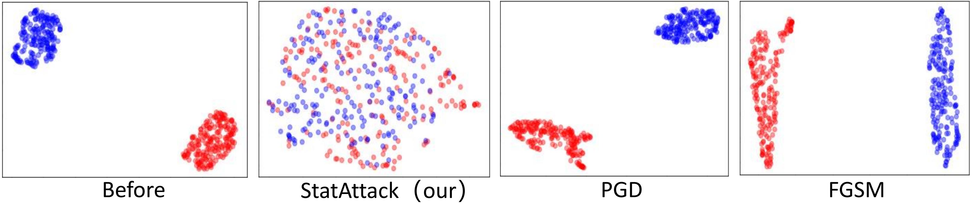
Figure 8: Feature distributions on ResNet after various attacks. Red and blue points represent feature distributions of attacked fake and real images, respectively. It is evident that the baseline attacks fail to align the feature distributions of fake and real images, whereas the proposed method can.

6.3 Attack on Frequency-based Detectors

To further demonstrate the attack capability of our method, we evaluate its effectiveness on two frequency-based detectors, namely DCTA [10] and DFTD [53]. As shown in the first column of Table 4, the attack success rates of our proposed attack are significantly higher than those of baseline attacks in both white-box and black-box settings. Moreover, our method can alter the frequency components of the fake images, resulting in generated adversarial examples closer to natural images in terms of frequency information. Therefore, the adversarial examples crafted from the spatial-based detector can also transfer to the frequency-based detectors, leading to the transferability in a broader sense. To demonstrate this, we used adversarial examples crafted from a spatial-based detector to attack frequency-based detectors. As shown in the last three columns of Table 4, the transfer attack success rate of our proposed attack significantly outperforms that of the baseline attacks.

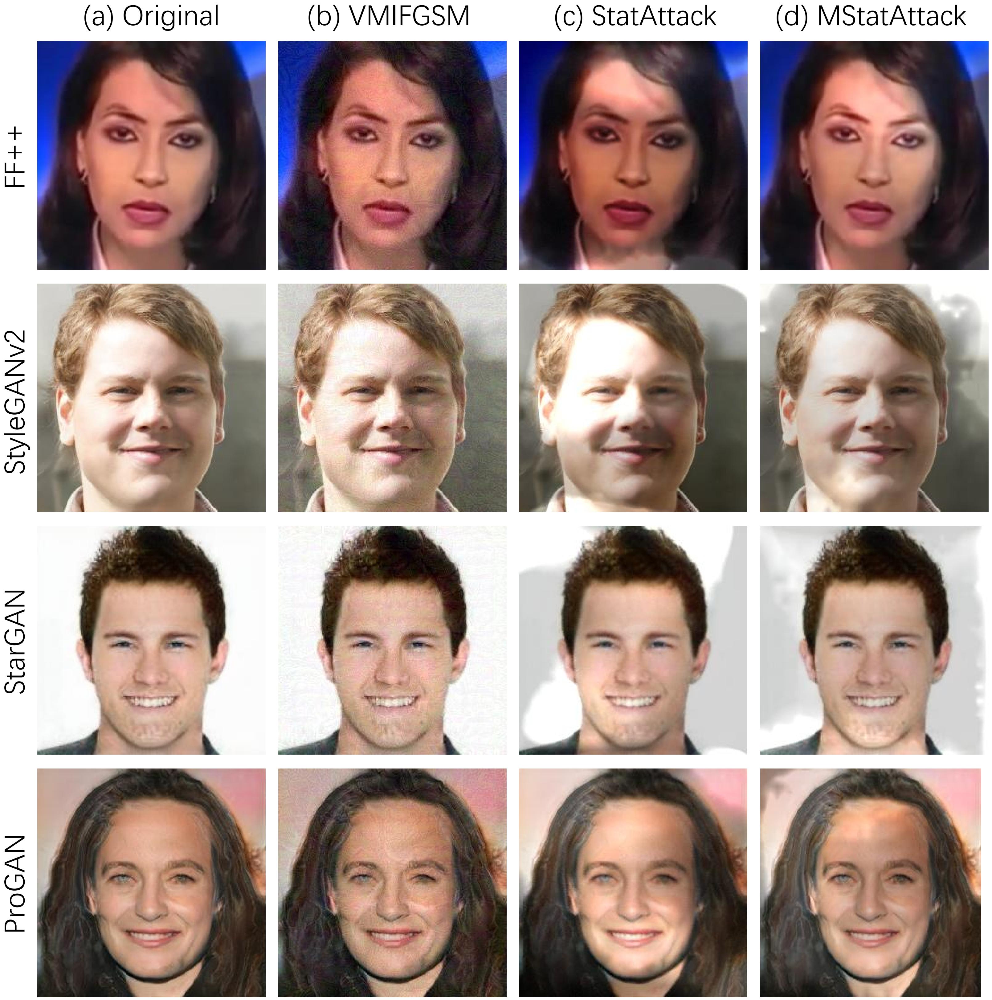
Figure 9: Visualization of the crafted adversarial examples. The visualizations include the raw fake images and the adversarial examples generated with VMIFGSM (b), StatAttack (c), and MStatAttack (d) on four datasets.

6.4 Images Quality Comparison

We also assess the image quality of the generated adversarial examples. The BRISQUE scores, shown in the last column of Tables 3 and 4, demonstrate that our attack method can maintain image quality while achieving high attack success rates. As illustrated in Figure 9, our method (i.e., StatAttack) can generates natural-looking adversarial examples, and that MStatAttack can further enhance the realism of the adversarial examples compared to StatAttack.

Table 5: Transfer success rate with different attack patterns. The adversarial examples are crafted from the ResNet.

Detector& Attack patterns	EfficientNet	DenseNet	MobileNet	DCTA	DFTD
only noise	22.5%	38.6%	32.4%	3.2%	4.8%
only exposure	26.8%	35.3%	36.6%	11.4%	14.2%
only blur	10.3%	11.7%	16.5%	8.5%	10.3%
w/o noise	37.5%	31.0%	43.4%	17.1%	20.5%
w/o exposure	39.5%	33.7%	40.5%	10.5%	13.3%
w/o blur	57.1%	70.3%	65.4%	10.7%	12.9%

6.5 Ablation Study

To assess the impact of each attack pattern on transferability, we perform transfer attack experiments using adversarial examples crafted from a spatial-based Deepfake detector ( i.e., ResNet ) in different attack patterns. Our results, as presented in Table 5, reveal that adversarial noise and adversarial exposure have the greatest impact on the spatial-based detectors. On the other hand, for frequency domain-based detectors, adversarial exposure and adversarial blur are the primary factors influencing the attack performance.

7 Conclusion

In this work, we propose a novel degradation-based attack method called StatAttack, which can be used to bypass various DeepFake detectors. StatAttack is capable of generating adversarial examples that closely resemble natural images in terms of feature distributions. In addition, we further extend StatAttack to a more powerful version, MStatAttack, which can select a more effective combination for attack and generate more natural-looking adversarial examples. We extensively evaluate our attack method on four spatial-based detectors and two frequency-based detectors using four datasets. The experimental results demonstrate the effectiveness of our attack method in both white-box and black-box settings.

Limitations. One limitation of our study is that we only considered three types of degradations. To enhance the robustness of our method, future work will focus on exploring additional natural degradations that could be more effective in simulating real-world scenarios. We also plan to leverage meta-learning to enhance the efficiency of our attack.

Social impacts. Our proposed attack method is capable of generating natural-looking adversarial examples that can transfer across different DeepFake detectors, posing a significant practical threat to the current DNN-based DeepFake detectors. This stealthy and transferable attack method can be employed to evaluate the robustness of Deepfake detectors in real-world applications or improve their robustness through adversarial training.

8 Supplementary Material

In the main paper, we have reported the attack results on various DeepFake detectors and compared the transferability and image quality with four baseline attacks. In the supplementary material, (1) We describe in detail the polynomial model and the smoothing function used to generate the adversarial exposure. (2) For the adversarial blur, we visualize the attack effect of adversarial Gaussian blur with different kernel sizes. (3) We show more image quality comparisons with baseline attacks. (4) We provide more implementation details.

8.1 Polynomial Model

The model provided by Gao et al. [13] consists of two parts, the first part is a polynomial model for generating the exposure, and the second part is a smoothing formula that maintains the naturalness of the exposure. The polynomial model is shown below:

$$\tilde{\mathbf{E_{i}}}=\sum_{t=0}^{D}\sum_{l=0}^{D-t}a_{t,l}T_{\varphi}\left(x_{i}\right)^{t}T_{\varphi}\left(y_{i}\right)^{l}$$ (9)

Where the "$\tilde{\cdot}$" presents the logarithmic operations, $\left\{a_{t,l}\right\}$ and $D$ denote the parameters and degree of the polynomial model, respectively. The number of parameters are $\left|\left\{a_{t,l}\right\}\right|=\frac{(D+1)(D+2)}{2}$, the lower degree $D$ leads to less model parameters $\left\{a_{t,l}\right\}$. $T_{\varphi}\left(\cdot\right)$ is the offset transformation with $\varphi$ being the control points. We denote $i$ as the $i$-th pixel, and its corresponding coordinate as $\left(x_{i},y_{i}\right)$. The $\left(T_{\varphi}\left(x_{i}\right),T_{\varphi}\left(y_{i}\right)\right)$ indicates that the exposure field is warped by offsetting the control points of each coordinate. In addition, The polynomial model with fewer parameters $\left\{a_{t,l}\right\}$ leads to a smoother exposure field. For convenient representations, we concatenate $\left\{a_{t,l}\right\}$ as a. We can maintain the smoothness of the generated exposure by restricting the a and $\varphi$, and the smoothing function can be written as follow:

$$S\left(\textbf{a},\varphi\right)=-\lambda_{a}\left\|\textbf{a}\right\|_{2}^{2}-\lambda_{\varphi}\left\|\bigtriangledown\varphi\right\|_{2}^{2}$$ (10)

The first term is to maintain the sparsity of a and thus ensure the smoothness of the generated adversarial exposure. The second term is to force the control point $\varphi$ to vary in a smaller range, encouraging a minor warping of the adversarial exposure field. The hyper-parameters $\lambda_{a}$ and $\lambda_{b}$ are used to regulate the balance between adversarial attack and smoothness. In detail, we initialize a be a vector whose entries share a common value (e.g., 0), the a and $\varphi$ are then gradually optimized in each attack iteration to produce smooth and effective adversarial exposure.

8.2 Different Kernel Sizes

The success of adversarial Gaussian blur is dependent on the size of the Gaussian kernel and the value of $\sigma$. While a larger Gaussian kernel and $\sigma$ can improve the success rate of transfer attacks, they can also result in more blurry images. To illustrate this point, we present a visualization of the adversarial examples generated by adversarial Gaussian blur using different kernel sizes, as shown in Figure 10.

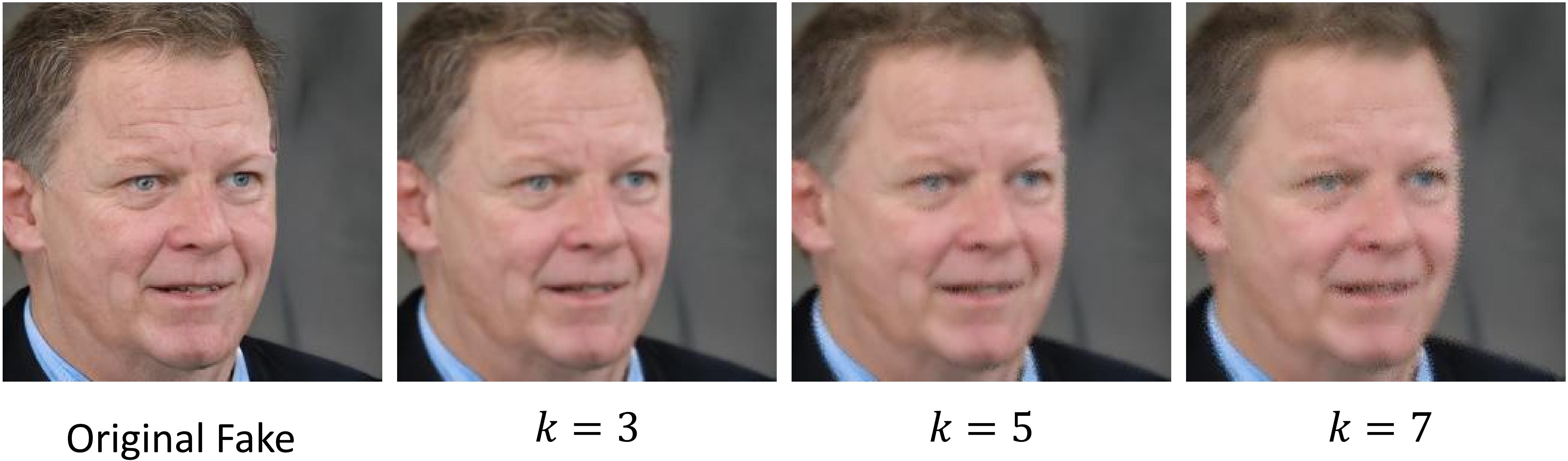
Figure 10: Adversarial examples generated by adversarial Gaussian blur with different kernel sizes. From left to right are the original image and the generated adversarial example with the Gaussian kernel size $k$ set to 3,5, and 7, respectively.

8.3 Additional Quality Comparisons

As shown in Figure 11, we provide more quality comparisons of the adversarial samples generated with the baseline attacks i.e. PGD[35], FGSM[16], MIFGSM[7] and VMIFGSM[50].

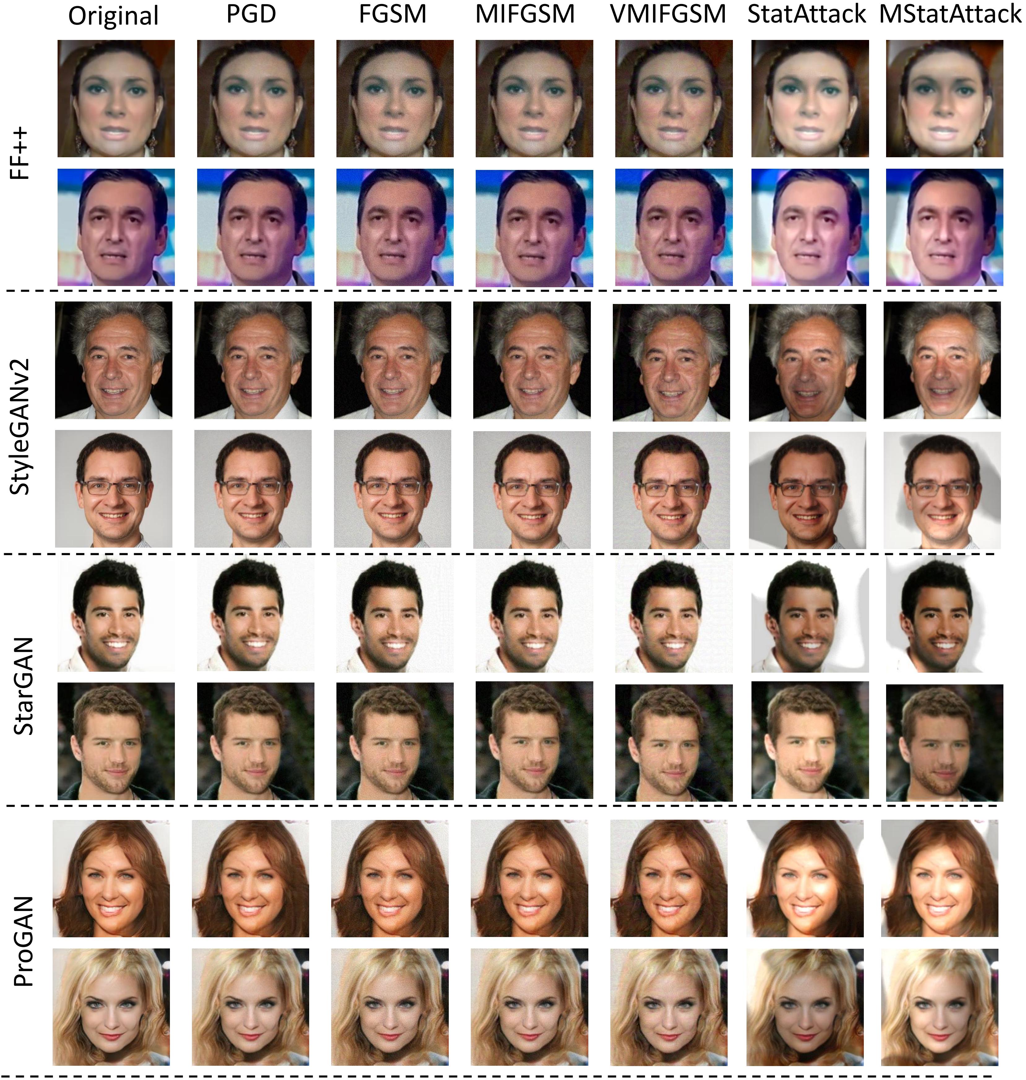
Figure 11: Visualization of generated adversarial examples. It contains the original fake image and the generated adversarial examples with the PGD, FGSM, MIFGSM, VMIFGSM, StatAttack, and MStatAttack on four datasets.

8.4 More Implementation Details

In our experiments, To balance the effectiveness of the attack and the quality of generated adversarial examples, we set the degree (i.e. $D$) of the polynomial model to 11, the learning rate of a and $\varphi$ is $10^{-2}$ and $10^{-3}$, respectively. For adversarial Gaussian blur, we set the Gaussian kernel size $k$ to 3. All the experiments were performed on a server running Ubuntu 6.0.8-arch1-1 system on a 10-core 3.60 GHz i9-10850k CPU with 31 GB RAM and an NVIDIA GeForce RTX 3090 GPU with 24 GB memory.

References

- [1] Mauro Barni, Kassem Kallas, Ehsan Nowroozi, and Benedetta Tondi. Cnn detection of gan-generated face images based on cross-band co-occurrences analysis. In 2020 IEEE International Workshop on Information Forensics and Security (WIFS), pages 1–6. IEEE, 2020.
- [2] Nicholas Carlini and Hany Farid. Evading deepfake-image detectors with white-and black-box attacks. In Proceedings of the IEEE/CVF conference on computer vision and pattern recognition workshops, pages 658–659, 2020.
- [3] Nicholas Carlini and David Wagner. Towards evaluating the robustness of neural networks. In 2017 ieee symposium on security and privacy (sp), pages 39–57. Ieee, 2017.
- [4] Shuyu Cheng, Yinpeng Dong, Tianyu Pang, Hang Su, and Jun Zhu. Improving black-box adversarial attacks with a transfer-based prior. Advances in neural information processing systems, 32, 2019.
- [5] Yunjey Choi, Minje Choi, Munyoung Kim, Jung-Woo Ha, Sunghun Kim, and Jaegul Choo. Stargan: Unified generative adversarial networks for multi-domain image-to-image translation. In Proceedings of the IEEE conference on computer vision and pattern recognition, pages 8789–8797, 2018.
- [6] Deepfake. "faceswap". https://github.com/deepfakes/faceswap. Accessed 2022-10-21.
- [7] Yinpeng Dong, Fangzhou Liao, Tianyu Pang, Hang Su, Jun Zhu, Xiaolin Hu, and Jianguo Li. Boosting adversarial attacks with momentum. In Proceedings of the IEEE conference on computer vision and pattern recognition, pages 9185–9193, 2018.
- [8] Ricard Durall, Margret Keuper, and Janis Keuper. Watch your up-convolution: Cnn based generative deep neural networks are failing to reproduce spectral distributions. In Proceedings of the IEEE/CVF conference on computer vision and pattern recognition, pages 7890–7899, 2020.
- [9] Gintare Karolina Dziugaite, Daniel M Roy, and Zoubin Ghahramani. Training generative neural networks via maximum mean discrepancy optimization. arXiv preprint arXiv:1505.03906, 2015.
- [10] Joel Frank, Thorsten Eisenhofer, Lea Schönherr, Asja Fischer, Dorothea Kolossa, and Thorsten Holz. Leveraging frequency analysis for deep fake image recognition. In International Conference on Machine Learning, pages 3247–3258. PMLR, 2020.
- [11] Apurva Gandhi and Shomik Jain. Adversarial perturbations fool deepfake detectors. In 2020 International joint conference on neural networks (IJCNN), pages 1–8. IEEE, 2020.
- [12] Gege Gao, Huaibo Huang, Chaoyou Fu, Zhaoyang Li, and Ran He. Information bottleneck disentanglement for identity swapping. In Proceedings of the IEEE/CVF Conference on Computer Vision and Pattern Recognition, pages 3404–3413, 2021.
- [13] Ruijun Gao, Qing Guo, Felix Juefei-Xu, Hongkai Yu, Huazhu Fu, Wei Feng, Yang Liu, and Song Wang. Can you spot the chameleon? adversarially camouflaging images from co-salient object detection. In Proceedings of the IEEE/CVF Conference on Computer Vision and Pattern Recognition, pages 2150–2159, 2022.
- [14] Yue Gao, Fangyun Wei, Jianmin Bao, Shuyang Gu, Dong Chen, Fang Wen, and Zhouhui Lian. High-fidelity and arbitrary face editing. In Proceedings of the IEEE/CVF Conference on Computer Vision and Pattern Recognition, pages 16115–16124, 2021.
- [15] Ian Goodfellow, Jonathon Shlens, and Christian Szegedy. Explaining and harnessing adversarial examples. In International Conference on Learning Representations, 2015.
- [16] Ian J Goodfellow, Jonathon Shlens, and Christian Szegedy. Explaining and harnessing adversarial examples. arXiv preprint arXiv:1412.6572, 2014.
- [17] Arthur Gretton, Karsten Borgwardt, Malte Rasch, Bernhard Schölkopf, and Alex Smola. A kernel method for the two-sample-problem. Advances in neural information processing systems, 19, 2006.
- [18] Chuan Guo, Jacob Gardner, Yurong You, Andrew Gordon Wilson, and Kilian Weinberger. Simple black-box adversarial attacks. In International Conference on Machine Learning, pages 2484–2493. PMLR, 2019.
- [19] Qing Guo, Felix Juefei-Xu, Xiaofei Xie, Lei Ma, Jian Wang, Bing Yu, Wei Feng, and Yang Liu. Watch out! motion is blurring the vision of your deep neural networks. Advances in Neural Information Processing Systems, 33:975–985, 2020.
- [20] Kaiming He, Xiangyu Zhang, Shaoqing Ren, and Jian Sun. Deep residual learning for image recognition. In Proceedings of the IEEE conference on computer vision and pattern recognition, pages 770–778, 2016.
- [21] Zhenliang He, Wangmeng Zuo, Meina Kan, Shiguang Shan, and Xilin Chen. Attgan: Facial attribute editing by only changing what you want. IEEE transactions on image processing, 28(11):5464–5478, 2019.
- [22] Andrew G Howard, Menglong Zhu, Bo Chen, Dmitry Kalenichenko, Weijun Wang, Tobias Weyand, Marco Andreetto, and Hartwig Adam. Mobilenets: Efficient convolutional neural networks for mobile vision applications. arXiv preprint arXiv:1704.04861, 2017.
- [23] Gao Huang, Zhuang Liu, Laurens Van Der Maaten, and Kilian Q Weinberger. Densely connected convolutional networks. In Proceedings of the IEEE conference on computer vision and pattern recognition, pages 4700–4708, 2017.
- [24] Yihao Huang, Felix Juefei-Xu, Qing Guo, Yang Liu, and Geguang Pu. Fakelocator: Robust localization of gan-based face manipulations. IEEE Transactions on Information Forensics and Security, 2022.
- [25] Shehzeen Hussain, Paarth Neekhara, Malhar Jere, Farinaz Koushanfar, and Julian McAuley. Adversarial deepfakes: Evaluating vulnerability of deepfake detectors to adversarial examples. In Proceedings of the IEEE/CVF winter conference on applications of computer vision, pages 3348–3357, 2021.
- [26] Andrew Ilyas, Logan Engstrom, Anish Athalye, and Jessy Lin. Black-box adversarial attacks with limited queries and information. In International Conference on Machine Learning, pages 2137–2146. PMLR, 2018.
- [27] Hyeonseong Jeon, Youngoh Bang, and Simon S Woo. Fdftnet: Facing off fake images using fake detection fine-tuning network. In IFIP International Conference on ICT Systems Security and Privacy Protection, pages 416–430. Springer, 2020.
- [28] Shuai Jia, Chao Ma, Taiping Yao, Bangjie Yin, Shouhong Ding, and Xiaokang Yang. Exploring frequency adversarial attacks for face forgery detection. In Proceedings of the IEEE/CVF Conference on Computer Vision and Pattern Recognition, pages 4103–4112, 2022.
- [29] Xiaojun Jia, Xingxing Wei, Xiaochun Cao, and Xiaoguang Han. Adv-watermark: A novel watermark perturbation for adversarial examples. In Proceedings of the 28th ACM International Conference on Multimedia, pages 1579–1587, 2020.
- [30] Felix Juefei-Xu, Run Wang, Yihao Huang, Qing Guo, Lei Ma, and Yang Liu. Countering malicious deepfakes: Survey, battleground, and horizon. International Journal of Computer Vision, pages 1–57, 2022.
- [31] Tero Karras, Timo Aila, Samuli Laine, and Jaakko Lehtinen. Progressive growing of gans for improved quality, stability, and variation. arXiv preprint arXiv:1710.10196, 2017.
- [32] Tero Karras, Samuli Laine, and Timo Aila. A style-based generator architecture for generative adversarial networks. In Proceedings of the IEEE/CVF conference on computer vision and pattern recognition, pages 4401–4410, 2019.
- [33] Dongze Li, Wei Wang, Hongxing Fan, and Jing Dong. Exploring adversarial fake images on face manifold. In Proceedings of the IEEE/CVF Conference on Computer Vision and Pattern Recognition, pages 5789–5798, 2021.
- [34] Ming Liu, Yukang Ding, Min Xia, Xiao Liu, Errui Ding, Wangmeng Zuo, and Shilei Wen. Stgan: A unified selective transfer network for arbitrary image attribute editing. In Proceedings of the IEEE/CVF conference on computer vision and pattern recognition, pages 3673–3682, 2019.
- [35] Aleksander Madry, Aleksandar Makelov, Ludwig Schmidt, Dimitris Tsipras, and Adrian Vladu. Towards deep learning models resistant to adversarial attacks. In International Conference on Learning Representations, 2017.
- [36] Scott McCloskey and Michael Albright. Detecting gan-generated imagery using saturation cues. In 2019 IEEE international conference on image processing (ICIP), pages 4584–4588. IEEE, 2019.
- [37] Anish Mittal, Anush Krishna Moorthy, and Alan Conrad Bovik. No-reference image quality assessment in the spatial domain. IEEE Transactions on image processing, 21(12):4695–4708, 2012.
- [38] Paarth Neekhara, Brian Dolhansky, Joanna Bitton, and Cristian Canton Ferrer. Adversarial threats to deepfake detection: A practical perspective. In Proceedings of the IEEE/CVF conference on computer vision and pattern recognition, pages 923–932, 2021.
- [39] Yuval Nirkin, Yosi Keller, and Tal Hassner. Fsgan: Subject agnostic face swapping and reenactment. In Proceedings of the IEEE/CVF International Conference on Computer Vision, pages 7184–7193, 2019.
- [40] Guim Perarnau, Joost Van De Weijer, Bogdan Raducanu, and Jose M Álvarez. Invertible conditional gans for image editing. arXiv preprint arXiv:1611.06355, 2016.
- [41] Hua Qi, Qing Guo, Felix Juefei-Xu, Xiaofei Xie, Lei Ma, Wei Feng, Yang Liu, and Jianjun Zhao. Deeprhythm: Exposing deepfakes with attentional visual heartbeat rhythms. In Proceedings of the 28th ACM international conference on multimedia, pages 4318–4327, 2020.
- [42] Yuyang Qian, Guojun Yin, Lu Sheng, Zixuan Chen, and Jing Shao. Thinking in frequency: Face forgery detection by mining frequency-aware clues. In European Conference on Computer Vision, pages 86–103. Springer, 2020.
- [43] Andreas Rössler, Davide Cozzolino, Luisa Verdoliva, Christian Riess, Justus Thies, and Matthias Nießner. Faceforensics: A large-scale video dataset for forgery detection in human faces. arXiv preprint arXiv:1803.09179, 2018.
- [44] Yucheng Shi, Siyu Wang, and Yahong Han. Curls & whey: Boosting black-box adversarial attacks. In Proceedings of the IEEE/CVF Conference on Computer Vision and Pattern Recognition, pages 6519–6527, 2019.
- [45] Mingxing Tan and Quoc Le. Efficientnet: Rethinking model scaling for convolutional neural networks. In International conference on machine learning, pages 6105–6114. PMLR, 2019.
- [46] Justus Thies, Michael Zollhöfer, and Matthias Nießner. Deferred neural rendering: Image synthesis using neural textures. ACM Transactions on Graphics (TOG), 38(4):1–12, 2019.
- [47] Binyu Tian, Felix Juefei-Xu, Qing Guo, Xiaofei Xie, Xiaohong Li, and Yang Liu. Ava: Adversarial vignetting attack against visual recognition. In Zhi-Hua Zhou, editor, Proceedings of the Thirtieth International Joint Conference on Artificial Intelligence, IJCAI-21, pages 1046–1053. International Joint Conferences on Artificial Intelligence Organization, 8 2021. Main Track.
- [48] Sheng-Yu Wang, Oliver Wang, Richard Zhang, Andrew Owens, and Alexei A Efros. Cnn-generated images are surprisingly easy to spot… for now. In Proceedings of the IEEE/CVF conference on computer vision and pattern recognition, pages 8695–8704, 2020.
- [49] Wei Wang, Yuan Sun, and Saman Halgamuge. Improving mmd-gan training with repulsive loss function. arXiv preprint arXiv:1812.09916, 2018.
- [50] Xiaosen Wang and Kun He. Enhancing the transferability of adversarial attacks through variance tuning. In Proceedings of the IEEE/CVF Conference on Computer Vision and Pattern Recognition, pages 1924–1933, 2021.
- [51] Cihang Xie, Zhishuai Zhang, Yuyin Zhou, Song Bai, Jianyu Wang, Zhou Ren, and Alan L Yuille. Improving transferability of adversarial examples with input diversity. In Proceedings of the IEEE/CVF Conference on Computer Vision and Pattern Recognition, pages 2730–2739, 2019.
- [52] Liming Zhai, Qing Guo, Xiaofei Xie, Lei Ma, Yi Estelle Wang, and Yang Liu. A3gan: Attribute-aware anonymization networks for face de-identification. In Proceedings of the 30th ACM International Conference on Multimedia, pages 5303–5313, 2022.
- [53] Xu Zhang, Svebor Karaman, and Shih-Fu Chang. Detecting and simulating artifacts in gan fake images. In 2019 IEEE international workshop on information forensics and security (WIFS), pages 1–6. IEEE, 2019.