Transductive Few-shot Learning with Prototype-based Label Propagation by Iterative Graph Refinement

Abstract

Few-shot learning (FSL) is popular due to its ability to adapt to novel classes. Compared with inductive few-shot learning, transductive models typically perform better as they leverage all samples of the query set. The two existing classes of methods, prototype-based and graph-based, have the disadvantages of inaccurate prototype estimation and sub-optimal graph construction with kernel functions, respectively. In this paper, we propose a novel prototype-based label propagation to solve these issues. Specifically, our graph construction is based on the relation between prototypes and samples rather than between samples. As prototypes are being updated, the graph changes. We also estimate the label of each prototype instead of considering a prototype be the class centre. On mini-ImageNet, tiered-ImageNet, CIFAR-FS and CUB datasets, we show the proposed method outperforms other state-of-the-art methods in transductive FSL and semi-supervised FSL when some unlabeled data accompanies the novel few-shot task.

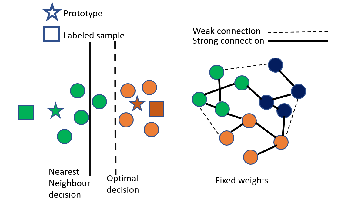
Figure 1: Drawbacks of prototype-based and graph-based FSL. (left) Some label assignments are incorrect due to the imperfect decision boundary. (right) Some “strong” links in the fixed graph are incorrect as they associate samples of different classes.

1 Introduction

With the availability of large-scale datasets and the rapid development of deep convolutional architectures, supervised learning exceeds in computer vision, voice, and machine translation [23]. However, lack of data makes the existing supervised models fail during the inference on novel tasks. As the annotation process may necessitate expert knowledge, annotations are may be scarce and costly (e.g., annotation of medical images). In contrast, humans can learn a novel concept from just a single example.

Few-shot learning (FSL) aims to mimic the capabilities of biological vision [7] and it leverages metric learning, meta-learning, or transfer learning. The purpose of metric-based FSL is to learn a mapping from images to an embedding space in which images from the same class are closer together and images from other classes are separated. Meta-learning FSL performs task-specific optimisation with the goal to generalize to other tasks well. Pre-training a feature extractor followed by adapting it for reuse on new class samples is an example of transfer learning.

Several recent studies [29, 11, 6, 13, 16, 35, 22, 34] explored transductive inference for few-shot learning. At the test time, transductive FSL infer the class label jointly for all the unlabeled query samples, rather than for one sample/episode at a time. Thus, transductive FSL typically outperforms inductive FSL. We categorise transductive FSL into: (i) FSL that requires the use of unlabeled data to estimate prototypes [44, 43, 26, 27, 2], and (ii) FSL that builds a graph with some kernel function and then uses label propagation to predict labels on query sets [29, 61, 22]. However, the above two paradigms have their own drawbacks. For prototype-based methods, they usually use the nearest neighbour classifier, which is based on the assumption that there exists an embedding where points cluster around a single prototype representation for each class. Fig. 1 (left) shows a toy example which is sensitive to the large within-class variance and low between-class variance. Thus, the two prototypes cannot be estimated perfectly by the soft label assignment alone. Fig. 1 (right) shows that Label-Propagation (LP) and Graph Neural Network (GNN) based methods depend on the graph construction which is commonly based on a specific kernel function determining the final result. If some nodes are wrongly and permanently linked, these connections will affect the propagation step.

In order to avoid the above pitfalls of transductive FSL, we propose prototype-based Label-Propagation (protoLP). Our transductive inference can work with a generic feature embedding learned on the base classes. Fig. 2 shows how to alternatively optimize a partial assignment between prototypes and the query set by (i) solving a kernel regression problem (or optimal transport problem) and (ii) a label probability prediction by prototype-based label propagation. Importantly, protoLP does not assume the uniform class distribution prior while significantly outperforming other methods that assume the uniform prior, as shown in ablations on the imbalanced benchmark [46] where methods relying on the balanced class prior fail. Our model outperforms state-of-the-art methods significantly, consistently providing improvements across different settings, datasets, and training models. Our transductive inference is very fast, with runtimes that are close to the runtimes of inductive inference.

Our contributions are as follows:

1. We identify issues resulting from separation of prototype -based and label propagation methods. We propose prototype-based Label Propagation (protoLP) for transductive FSL, which unifies both models into one framework. Our protoLP estimates prototypes not only from the partial assignment but also from the prediction of label propagation. The graph for label propagation is not fixed as we alternately learn prototypes and the graph.

2. By introducing parameterized label propagation step, we remove the assumption of uniform class prior while other methods highly depend on this prior.

3. We showcase advantages of protoLP on four datasets for transductive and semi-supervised learning, Our protoLP outperforms the state of the art under various settings including different backbones, unbalanced query set, and data augmentation.

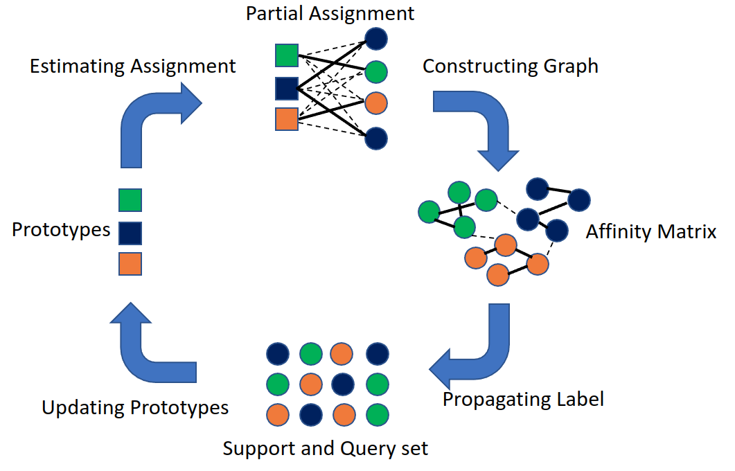
Figure 2: Our transductive few-shot learning: (i) based on prototypes, estimate as partial assignment (one can use soft k-means in Eq. (4) instead); (ii) a graph is constructed by the assignment, followed by the prototype-based label propagation, predicting the label soft score; (ii) updating prototypes based on the prediction.

2 Related Work

Few-shot classification methods often exploit the meta-learning paradigm [47, 44, 36], and they use episodes for training and testing. Approaches [50, 4] show that meta-training is not required for learning good features for few-shot learning. Instead, they train a typical classification network with two blocks: the feature extractor and the classification head. Many FSL models combine backbone with classification head [19, 42, 55, 49, 48], detection head [56, 58, 57], localization head [30] or detection head [15].

We focus on designing the inference stage and improving its performance in transductive and semi-supervised setting.

Graph-based FSL often form a graph via an adjacency matrix based on Radial Basis Function (RBF), used in the propagation of labels or features. Satorras et al. [40] propagate labels by building an affinity matrix between the support set and the unlabeled data. wDAE-GNN [9] generates classification weights with a graph neural network (GNN) and applies a denoising AutoEncoder (DAE) to regularize the representation. Approach [29] learns propagation. Embedding Propagation [38] propagates labels and the embedding to decrease the intra-class distance. Set-to-set functions have also been used for embedding adaptation [54].

In contrast to FSL with a fixed graph, we do not construct a graph from samples directly but construct a bipartite graph by prototypes and samples. As prototypes change, so does the constructed graph, which we regard as a learnable graph.

Transductive and Semi-Supervised Few-Shot Learning is not as popular as inductive FSL which only uses samples in the support set to fine-tune the model or learn a function for the inference of query labels. In contrast, transductive FSL enjoys access to all the query data. In this paper, we categorise transductive FSL into (i) prototype-based and (ii) label propagation based FSL. Prototypical Network [44] learns a metric space in which classification is performed by computing distances to prototype representations of each class. Simon et al. [43] use adaptive subspace-based prototypes. Lichtenstein et al. [26] employ subspace learning via PCA or ICA to extract discriminant features for the nearest neighbour classifier on prototypes. Liu et al. [27] improve prototype estimation. TIM [2] maximizes the mutual information between the query features and their label predictions for a few-shot task at inference, while minimizing the cross-entropy loss on the support set to estimate prototypes. Label Propagation (LP) is popular in transductive FSL methods [29, 3, 61, 22, 60], which construct a graph from the support set and the entire query set, and propagate labels within the graph. However, as in graph-based FSL methods, LP employs kernel functions (RBF or cosine) to construct the graph between samples. Additionally, some methods [14, 22, 60] leverage the uniform prior on the class distribution with the optimal transport while in realistic evaluation of transductive FSL the prior is unknown [46]. In semi-supervised FSL [29, 25, 37, 43], the unlabeled data is provided in addition to the support set and is assumed to have a similar distribution to the target classes (although unrelated noisy samples may be also added).

3 Methodology

Below we introduce prototypical networks [44], explain semi-supervised prototype computation, and present transductive FSL based on label propagation. Then, we present our prototype-based Label Propagation (protoLP). Finally, we show how to optimize protoLP by updating the prototypes, solving the partial assignment problem and the label propagation by the linear projection. Moreover, we demonstrate how to obtain the final label prediction for the query set given learnt prototypes. Fig. 2 illustrates our method.

3.1 Preliminaries

Inductive FSL uses a support set of $K$ classes with $N$ labeled examples per class, $S\equiv\{(\mathbf{x}_{i},y_{i})\}_{i=1}^{L}$ where $L=NK$, each $\mathbf{x}_{i}\in\mathbb{R}^{D}$ is the $D$-dimensional feature vector (from backbone) of an example and $y_{i}\in\{1,\cdots,K\}$ is the corresponding label. $S_{k}\subset S$ is the set of examples labeled with class $k$. Prototypical networks [44] compute a prototype of class as the mean vector of support samples belonging to the class:

$$\mathbf{c}_{k}=\frac{1}{\left|S_{k}\right|}\sum_{\mathbf{x}:\,y(x)\in S_{k}}\mathbf{x}.$$ (1)

Given a distance function $d:\mathbb{R}^{D}\times\mathbb{R}^{D}\rightarrow\mathbb{R}^{+}$, prototypical nets use Nearest Class Mean (NCM) to predict the label of query $\mathbf{x}$:

$$k^{*}=\arg\min_{k}d\left(\mathbf{x},\mathbf{c}_{k}\right).$$ (2)

Transductive Few-shot Learning. In the case of inductive FSL, the prediction is performed independently on each episode, and thus the mean vector is only dependent on the support set of $N$ labeled examples, as shown in Eq. (1), and is fixed for the given embedded features. However, in the case of transductive FSL, the prediction is performed inclusive of all queries, $Q\equiv\{\mathbf{x}_{L+i}\}^{U}_{i=1}$, where $U=RK$, and the query set has $K$ classes with $R$ unlabeled examples per class.

Inference of Prototypes. Transductive/semi-supervised Prototypical Network [44] treats prototypes ${\bm{c}}_{k}$ in Eq. (1) as clusters. The unlabeled samples with indexes $L+1\leq i\leq L+U$ are soft-assigned [18] to each cluster $\mathbf{c}_{k}$, yielding $z_{ik}$, whereas labeled samples with indexes $1\leq i\leq L$ use one-hot labels, i.e., $z_{ik}=1\text{ for }k=y_{i}$ and $z_{ik}=0\text{ for }k\neq y_{i}$. Specifically, refined prototypes are obtained as follows:

$${\bm{c}}_{k} =\frac{\sum_{i=1}^{L}z_{ik}{\bm{x}}_{i}+\sum_{j=L+1}^{L+U}{z}_{jk}{\bm{x}}_{j}}{\sum_{i^{\prime}=1}^{L}z_{i^{\prime}k}+\sum_{j^{\prime}=L+1}^{L+U}{z}_{j^{\prime}k}}\qquad\text{where}$$ (3)

$${z}_{ik} =\begin{cases}\frac{\exp\left(-\lVert{\bm{x}}_{i}-{\bm{c}}_{k}\rVert_{2}^{2}\right)}{\sum_{k^{\prime}}\exp\left(-\lVert{\bm{x}}_{i}-\bm{c}_{k^{\prime}}\rVert_{2}^{2}\right)}\quad\text{if}\quad L+1\leq i\leq L+U\\ \text{OneHot}(y_{i})\quad\qquad\text{if}\quad 1\leq i\leq L.\end{cases}$$ (4)

The prediction of each query label follows Eq. (2). Notice that although the prototypes estimation leverages all data in the query set, the inference still only depends on prototypes and a single sample rather than prototypes and all samples.

Label Propagation. We form a graph $G=(\mathcal{V},\mathcal{E})$ where vertices $\mathcal{V}$ represent all labeled and unlabeled samples, and edges $\mathcal{E}$ are represented by a distance matrix ${\bm{W}}$. Let ${\bm{D}}$ be a diagonal matrix whose diagonal elements are given by $D_{ii}=\sum_{j}{W_{ij}}$. The graph Laplacian is then defined as ${\bm{L}}={\bm{D}}-{\bm{W}}$, which is used for smoothness-based regularization by taking into account the unlabeled data:

$$\frac{1}{2}\operatorname{Tr}(\tilde{{\bm{Y}}}^{\top}{\bm{L}}\tilde{{\bm{Y}}})=\frac{1}{2}\sum_{i,j}W_{ij}(\tilde{{\bm{y}}_{i}}-\tilde{{\bm{y}}_{j}})^{2}.$$ (5)

For practical reasons, Zhou et al. [59] are concerned not only with the smoothness but the impact of the supervised loss on the propagation. Thus, they minimize a combination of the smoothness and the squared error training loss:

$$\tilde{{\bm{Y}}}^{*}=\operatorname*{arg\,min}_{\tilde{{\bm{Y}}}}\sum_{i=1}^{L}\|\tilde{{\bm{y}}}_{i}-{\bm{y}}_{i}\|_{2}^{2}+\frac{\lambda}{2}\operatorname{Tr}(\tilde{{\bm{Y}}}^{\top}{\bm{L}}\tilde{{\bm{Y}}}).$$ (6)

Eq. (6) relies on the quality of a fixed Laplacian matrix ${\bm{L}}$ which largely determines the final performance of method.

3.2 Proposed Formulation

Below we introduce our prototype-based Label Propagation (protoLP). Firstly, we parameterize the label propagation step and explain why. Then, we explain how to use prototypes to construct a graph, and we combine the above two components into protoLP.

Parameterized Label Prediction. Given the adjacency matrix ${\bm{W}}$, we can solve label propagation by Eq. (6). However, we introduce a linear projection ${\bm{A}}$ into the label propagation step to limit overfitting to matrix ${\bm{W}}$. Let:

$$\tilde{{\bm{Y}}}={\bm{Z}}{\bm{A}},$$ (7)

where ${\bm{A}}=[{\bm{a}}_{1},\cdots,{\bm{a}}_{K}]^{\top}$ has $K$ basis functions and ${\bm{Z}}$ comes from Eq. (4) given a prototype set $\{{\bm{c}}_{k}\}_{k=1}^{K}$. Substitute Eq. (7) into Eq. (6), we obtain:

$$\!\!\!\!{\bm{A}}^{*}\!=\mathop{\arg\min}_{{\bm{A}}}\left\|{\bm{Z}}_{L}{\bm{A}}-{\bm{Y}}_{L}\right\|^{2}_{F}+\frac{\lambda}{2}\operatorname{Tr}({\bm{A}}^{\top}{\bm{Z}}^{\top}{\bm{L}}{\bm{Z}}{\bm{A}}),$$ (8)

where ${\bm{Z}}_{L}\!=\![{\bm{z}}_{1},\dots,{\bm{z}}_{L}]^{\top}\!\in\!\mathbb{R}^{L\times K}$. ${\bm{Y}}_{L}\!=\![{\bm{y}}_{1},\dots,{\bm{y}}_{L}]^{\top}\!\in\!\mathbb{R}^{L\times K}$ is the submatrix according to the assignment and label partition. Intuitively, we can regard ${\bm{a}}_{k}$ as a learnable label for the $k$-th prototype which is non-sparse in contrast to a one-hot class vector. Based on the above model, one can estimate a soft score of likely category of an inaccurate prototype.

Prototype-based Graph Construction. Prototype-based graphs are based on the idea that we can use a small number of prototypes to turn sample-to-sample affinity computations into much simpler sample-to-prototype affinity computations [28]. Below we explain how to construct a graph with prototypes. Given a prototype set $\{{\bm{c}}_{k}\}_{k=1}^{K}$, for each sample we obtain a partial assignment ${\bm{z}}_{j}$ with soft assignment in Eq. (4). We form the adjacency matrix ${\bm{W}}$ as:

$${\bm{W}}={\bm{Z}}\mathbf{\Lambda}^{-1}{\bm{Z}}^{\top},$$ (9)

where the diagonal matrix $\mathbf{\Lambda}\in\mathbb{R}^{K\times K}$ is defined as $\Lambda_{kk}=\sum_{i}Z_{ik}$ (index $i$ iterates over all samples). The corresponding Laplacian matrix is ${\bm{L}}={\bm{I}}-{\bm{Z}}\mathbf{\Lambda}^{-1}{\bm{Z}}^{\top}$. $W_{ij}$ captures relation between the $i$-th and $j$-th samples by confounding variables $\mathbf{c}_{k}$ according to the chain rule of Markov random walks:

$$W_{ij}\!=\!p\left({\bm{x}}_{i}\!\mid\!{\bm{x}}_{j}\right) =\sum_{k=1}^{K}p\left({\bm{x}}_{i}\!\mid\!{\bm{c}}_{k}\right)p\left({\bm{c}}_{k}\!\mid\!{\bm{x}}_{j}\right)\!=\!p\left({\bm{x}}_{j}\!\mid\!{\bm{x}}_{i}\right)$$ (10)

$$=\sum_{k=1}^{K}\frac{z_{jk}}{\sum_{j^{\prime}}z_{j^{\prime}k}}z_{i,k}=\sum_{k=1}^{K}\frac{z_{ik}z_{jk}}{\Lambda_{kk}},$$

where $p({\bm{x}}_{i}\!\mid\!{\bm{c}}_{k})\!=\!Z_{ik}$ and $W_{ij}\!=\!W_{ji}$. One may think of the above process as a 2-hop diffusion on a bipartite graph with samples $\mathbf{x}_{i}$ and prototypes $\mathbf{c}_{k}$ located in two partitions of that graph. Notice the graph changes with prototypes.

Prototype-based Label Propagation (protoLP). Based on parameterized label prediction and prototype-based graph construction, we combine Eq. (8) and (9) into:

$$\!\!\!\!\min_{{\bm{A}}}\frac{1}{2}\left\|{\bm{Z}}_{L}{\bm{A}}-{\bm{Y}}_{L}\right\|^{2}_{F}+\frac{\lambda}{2}\operatorname{Tr}({\bm{A}}^{\top}{\bm{Z}}^{\top}({\bm{I}}-{\bm{Z}}\mathbf{\Lambda}^{-1}{\bm{Z}}^{\top}){\bm{Z}}{\bm{A}}).$$ (11)

As Eq. (8) and (9) are highly dependent on prototypes, instead of using the update of $\mathbf{c}_{k}$ as in Eq. (4), we use steps from Section 3.3. Firstly, we initialize each prototype as the mean vector of the support samples belonging to its class.

Input: ${\bm{X}},{\bm{Y}},\lambda,\alpha,n_{\text{step}}$

Init: $\mathbf{\tilde{c}}_{k}=\frac{1}{\left|S_{k}\right|}\sum_{\left({\bm{x}}_{i},y_{i}\right)\in S_{k}}{\bm{x}}_{i}$,$k=0$;

while $k<n_{\text{step}}$ do

       Estimating Assignment:

       $\;\;{Z}_{ij}=\frac{\exp(-\left\|{\bm{x}}_{i}-\tilde{{\bm{c}}}_{j}\right\|^{2}_{2})}{\sum_{j^{\prime}}exp(-\left\|{\bm{x}}_{i}-\tilde{{\bm{c}}}_{j^{\prime}}\right\|^{2}_{2})}$;

       Constructing Graph:

       $\;\;\Lambda_{kk}=\sum_{i}Z_{ik}$ and ${\bm{W}}=\bm{Z}_{t}\bm{\Lambda}^{-1}\bm{Z}^{\top}_{t}$;

       Propagating Label:

       $\;\;\tilde{\mathbf{Y}}=\bm{Z}_{t}\left(\bm{Z}_{L}^{\top}\bm{Z}_{L}+\lambda\bm{Z}^{\top}_{t}\left(\bm{I}-{\bm{W}}\right)\bm{Z}_{t}\right)^{-1}\bm{Z}^{\top}_{t}\bm{Y}$;

       Updating Prototypes:

       $\;\;\mathbf{\tilde{C}}\leftarrow(1-\alpha)\mathbf{\tilde{C}}+\alpha\tilde{{\bm{Y}}}{\bm{X}}$;

       $k\leftarrow k+1$

end while

return $y_{i}=\operatorname*{arg\,max}_{j}{\tilde{Y}}_{i,j}$

Algorithm 1 Prototype-based Label Propagation.

Table 1: Comparison of test accuracy against state-of-the-art methods for 1-shot and 5-shot classification. (^∗: inference aug., §4.2.3)

			mini-ImageNet		tiered-ImageNet
Methods	Setting	Network	1-shot	5-shot	1-shot	5-shot
MAML [8]	Inductive	ResNet-18	49.61 $\pm$ 0.92	65.72 $\pm$ 0.77	–	–
RelationNet [45]	Inductive	ResNet-18	52.48 $\pm$ 0.86	69.83 $\pm$ 0.68	–	–
MatchingNet [47]	Inductive	ResNet-18	52.91 $\pm$ 0.88	68.88 $\pm$ 0.69	–	–
ProtoNet [44]	Inductive	ResNet-18	54.16 $\pm$ 0.82	73.68 $\pm$ 0.65	–	–
TPN [29]	transductive	ResNet-12	59.46	75.64	–	–
TEAM [35]	transductive	ResNet-18	60.07	75.9	–	–
Transductive tuning [6]	Transductive	ResNet-12	62.35 $\pm$ 0.66	74.53 $\pm$ 0.54	–	–
MetaoptNet [24]	Transductive	ResNet-12	62.64 $\pm$ 0.61	78.63 $\pm$ 0.46	65.99 $\pm$ 0.72	81.56 $\pm$ 0.53
CAN+T [11]	Transductive	ResNet-12	67.19 $\pm$ 0.55	80.64 $\pm$ 0.35	73.21 $\pm$ 0.58	84.93 $\pm$ 0.38
DSN-MR [43]	Transductive	ResNet-12	64.60 $\pm$ 0.72	79.51 $\pm$ 0.50	67.39 $\pm$ 0.82	82.85 $\pm$ 0.56
ODC∗ [34]	Transductive	ResNet-18	77.20 $\pm$ 0.36	87.11 $\pm$ 0.42	83.73 $\pm$ 0.36	90.46 $\pm$ 0.46
MCT∗ [21]	Transductive	ResNet-12	78.55 $\pm$ 0.86	86.03 $\pm$ 0.42	82.32 $\pm$ 0.81	87.36 $\pm$ 0.50
EASY∗[1]	Transductive	ResNet-12	82.31 $\pm$ 0.24	88.57 $\pm$ 0.12	83.98 $\pm$ 0.24	89.26 $\pm$ 0.14
protoLP (ours)	Transductive	ResNet-12	70.77 $\pm$ 0.30	80.85 $\pm$ 0.16	84.69 $\pm$ 0.29	89.47 $\pm$ 0.15
protoLP∗ (ours)	Transductive	ResNet-12	84.35 $\pm$ 0.24	90.22 $\pm$ 0.11	86.27 $\pm$ 0.25	91.19 $\pm$ 0.14
protoLP (ours)	Transductive	ResNet-18	75.77 $\pm$ 0.29	84.00 $\pm$ 0.16	82.32 $\pm$ 0.27	88.09 $\pm$ 0.15
protoLP∗ (ours)	Transductive	ResNet-18	85.13 $\pm$ 0.24	90.45 $\pm$ 0.11	83.05 $\pm$ 0.25	88.62 $\pm$ 0.14
ProtoNet [44]	Inductive	WRN-28-10	62.60 $\pm$ 0.20	79.97 $\pm$ 0.14	–	–
MatchingNet [47]	Inductive	WRN-28-10	64.03 $\pm$ 0.20	76.32 $\pm$ 0.16	–	–
SimpleShot [50]	Inductive	WRN-28-10	65.87 $\pm$ 0.20	82.09 $\pm$ 0.14	70.90 $\pm$ 0.22	85.76 $\pm$ 0.15
S2M2-R [31]	Inductive	WRN-28-10	64.93 $\pm$ 0.18	83.18 $\pm$ 0.11	-	-
Transductive tuning [6]	Transductive	WRN-28-10	65.73 $\pm$ 0.68	78.40 $\pm$ 0.52	73.34 $\pm$ 0.71	85.50 $\pm$ 0.50
SIB [13]	Transductive	WRN-28-10	70.00 $\pm$ 0.60	79.20 $\pm$ 0.40	–	–
BD-CSPN [27]	Transductive	WRN-28-10	70.31 $\pm$ 0.93	81.89 $\pm$ 0.60	78.74 $\pm$ 0.95	86.92 $\pm$ 0.63
EPNet [38]	Transductive	WRN-28-10	70.74 $\pm$ 0.85	84.34 $\pm$ 0.53	78.50 $\pm$ 0.91	88.36 $\pm$ 0.57
LaplacianShot [61]	Transductive	WRN-28-10	74.86 $\pm$ 0.19	84.13 $\pm$ 0.14	80.18 $\pm$ 0.21	87.56 $\pm$ 0.15
ODC [34]	Transductive	WRN-28-10	80.22	88.22	84.70	91.20
iLPC [22]	Transductive	WRN-28-10	83.05 $\pm$ 0.79	88.82 $\pm$ 0.42	88.50 $\pm$ 0.75	92.46 $\pm$ 0.42
protoLP (ours)	Transductive	WRN-28-10	83.07 $\pm$ 0.25	89.04 $\pm$ 0.13	89.04 $\pm$ 0.23	92.80 $\pm$ 0.13
protoLP* (ours)	Transductive	WRN-28-10	84.32 $\pm$ 0.21	90.02 $\pm$ 0.12	89.65 $\pm$ 0.22	93.21 $\pm$ 0.13

3.3 Optimization

Below we explain how to optimize w.r.t. ${\bm{Z}},{\bm{A}}$ and ${\bm{C}}$ by alternating. The order of optimisation in each round assumes minimization w.r.t. ${\bm{Z}}$, then ${\bm{A}}$ and finally ${\bm{C}}$.

Updating $\mathbf{Z}$. Firstly, given a prototype set $\{{\bm{c}}_{k}\}_{k=1}^{K}$, we optimize the following equation w.r.t. $\mathbf{Z}$:

$$\mathbf{Z}_{t}=\operatorname*{arg\,min}_{{\bm{Z}}}\sum_{i,k}z_{ik}\|{\bm{x}}_{i}-{\bm{c}}_{k}\|^{2}_{2},\;\text{s.t.}\;\sum_{k}{\bm{z}}_{ik}\!=\!1.$$ (12)

Eq. (12) can be solved by Eq. (4).

Updating $\mathbf{A}$. Next, we solve Eq. (11) w.r.t. $\mathbf{A}$ by globally-optimal closed-form formula:

$$\!\!\!\!{\bm{A}}_{t}\!=\!\left({\bm{Z}}_{L}^{\top}{\bm{Z}}_{L}+\lambda{\bm{Z}}_{t}^{\top}\!\left({\bm{I}}-{\bm{Z}}_{t}\mathbf{\Lambda}^{-1}{\bm{Z}}_{t}^{\top}\right){\bm{Z}}_{t}\right)^{-1}\!{\bm{Z}}_{t}^{\top}{\bm{Y}}.$$ (13)

Subsequently, we can infer the label soft score by Eq. (7), i.e., $\tilde{{\bm{Y}}}_{t}={\bm{Z}}_{t}{\bm{A}}_{t}$ is the output for updating prototypes in the next iteration. Substituting Eq. (13) into (7), we have:

$$\mathbf{\tilde{Y}}_{t}={\bm{Z}}_{t}({\bm{Z}}_{L}^{\top}{\bm{Z}}_{L}+\lambda{\bm{Z}}_{t}^{\top}\left({\bm{I}}-{\bm{Z}}_{t}\mathbf{\Lambda}^{-1}{\bm{Z}}_{t}^{\top}\right){\bm{Z}}_{t})^{-1}{\bm{Z}}_{t}^{\top}{\bm{Y}}.$$ (14)

Using ${\bm{A}}$ is not mandatory but this linear projection improves results by limiting overfitting during propagation.

Updating $\mathbf{C}$. We update $\mathbf{C}$ by:

$$\mathbf{C}_{t} =\operatorname*{arg\,min}_{\mathbf{C}}\sum_{i,k}\tilde{y}_{ik}\|{\bm{x}}_{i}-{\bm{c}}_{k}\|^{2}_{2},$$ (15)

$$\!\!\!\!\!\text{where one may set }\;{\bm{c}}_{k}=\frac{\sum_{i=1}^{L}{\bm{x}}_{i}\tilde{y}_{ik}+\sum_{j=L+1}^{L+U}{\bm{x}}_{j}\tilde{y}_{jk}}{\sum_{i^{\prime}=1}^{L}\tilde{y}_{i^{\prime}k}+\sum_{j^{\prime}=L+1}^{L+U}\tilde{y}_{j^{\prime}k}}.$$ (16)

We use the gradient decent and the exponential running average to update ${\bm{C}}$ to avoid instability that changing $\tilde{{\bm{Y}}}$ may pose:

$$\mathbf{C}_{t}=(1-\alpha)\mathbf{C}_{t-1}+\alpha\tilde{{\bm{Y}}}^{\top}\!{\bm{X}},$$ (17)

where $0\leq\alpha\leq 1$ controls the speed of adaptation of $\mathbf{C}_{t}$.

Inference. For each query ${\bm{x}}_{L+i}\!\in\!Q$ (note ${\bm{x}}_{1},\cdots,{\bm{x}}_{L}$ where $L\!=\!NK$ are for training, we predict its pseudo-label by $\operatorname*{arg\,max}\limits_{k\in\{1,\cdots,K\}}\tilde{y}_{jk}$ that corresponds to the maximum element of the $j$-th row of the resulting matrix $\tilde{{\bm{Y}}}$.

Uniform Prior with Optimal Transport. In transductive FSL, the evaluation based on the balanced class setting is widely used. Thus many methods [22, 14, 60] leverage the prior of uniform distribution of class labels to improve the performance. We also consider this factor and normalize $\tilde{{\bm{Y}}}$ to a given row-wise sum $\mathbf{d}_{r}\in\mathbb{R}^{U}$ and column-wise sum $\mathbf{d}_{c}\in\mathbb{R}^{K}$. The normalization itself is a projection of $\tilde{{\bm{Y}}}$ onto the set $\mathbb{S}_{\mathbf{d}_{r},\mathbf{d}_{c}}$ of non-negative $U\times K$ matrices having row-wise sum $\mathbf{d}_{r}$ and column-wise sum $\mathbf{d}_{c}$:

$$\mathbb{S}_{\mathbf{d}_{r},\mathbf{d}_{c}}\!\equiv\!\left\{\tilde{{\bm{Y}}}\!\in\!\mathbb{R}^{U\times K}\!:\tilde{{\bm{Y}}}\mathbf{1}_{K}\!=\!\mathbf{d}_{r},\tilde{{\bm{Y}}}^{\top}\!\mathbf{1}_{U}\!=\!\mathbf{d}_{c}\right\}.$$ (18)

We use the Sinkhorn-Knopp algorithm [17] for this projection. It alternates (until convergence) between rescaling the rows of $\tilde{{\bm{Y}}}$ to add up to $\mathbf{d}_{r}$ and its columns to add up to $\mathbf{d}_{c}$:

$$\begin{array}[]{l}\tilde{{\bm{Y}}}\leftarrow\operatorname{diag}(\mathbf{d}_{r})\operatorname{diag}\left(\tilde{{\bm{Y}}}\mathbf{1}_{U}\right)^{-1}\tilde{{\bm{Y}}},\\ \tilde{{\bm{Y}}}\leftarrow\tilde{{\bm{Y}}}\operatorname{diag}\left(\tilde{{\bm{Y}}}^{\top}\mathbf{1}_{K}\right)^{-1}\operatorname{diag}(\mathbf{d}_{c}).\end{array}$$

For the uniform prior assumption, $\mathbf{d}_{c}={\bm{1}}_{U}$ and $\mathbf{d}_{c}=R\cdot{\bm{1}}_{K}$, where $R$ is the query number of each class.

Algorithm 1 summarizes our standard protoLP without the Sinkhorn-Knopp algorithm [5] omitted for brevity. Four steps indicated in italics are also indicated in Fig. 2.

4 Experiments

We evaluate our method on four few-shot classification benchmarks, mini-ImageNet [47], tiered-ImageNet [37], CUB [52] and CIFAR-FS [4, 20], all often used in transductive and semi-supervised FSL [16, 29, 35, 37, 43]. We use the standard evaluation protocols. The results of the transductive and semi-supervised FSL evaluation together with comparisons to previous methods are summarized in Tables 1, 3, 3, 4 and 5, and discussed below. The performance numbers are given as accuracy %, and the 0.95 confidence intervals are reported. The tests are performed on 10,000 randomly drawn 5-way episodes, with 1 or 5 shots (number of support examples per class), and with 15 queries per episode (unless otherwise specified). We use publicly available pre-trained backbones that are trained on the base class training set. We experiment with ResNet-12, ResNet-18 [33], and WRN-28-10 [39] backbones pre-trained in S2M2-R [31], and DenseNet [26] and MobileNet [12] pre-trained in SimpleShot [50].

4.1 FSL benchmarks used in our experiments

Transductive FSL Setting. We investigate transductive FSL with the set of queries as the source of unlabeled data, which is typical when an FSL classifier receives a bulk of the query data for an off-line evaluation. In Table 1, we report the performance of our protoLP, and compare it to baselines and state-of-the-art (SOTA) transductive FSL methods from the literature: TPN [29], Transductive FineTuning [6], MetaOptNet [24], DSN-MR [43], EPNet [38], CAN-T [11], SIB [53], BP-CSPN [29], LaplacianShot [61], RAP-LaplacianShot [10], ICI [51], TIM [2], iLPC [22], and PT-MAP [14]. We also compare to SOTA regular FSL based on S2M2-R [31] to highlight the effectiveness of using the unlabeled data. Tables 1, 3 and 3 show that on both transductive FSL benchmarks (mini-ImageNet and tiered-ImageNet), protoLP consistently outperforms all the previous (transductive and inductive) methods.

Our protoLP is insensitive to the feature extractor, e.g., see protoLP with DenseNet and MobileNet in Table 5. We used features from SimpleShot [50] backbones. Compared with SimpleShot, protoLP gains 13% and 3% on the 1- and 5-shot protocols. It also outperforms other transductive methods based on DenseNet such as LaplacianShot [61], RAP-LaplacianShot [10] and variants of TAFSSL [26].

Table 2: Test accuracy vs. the state of the art (transductive inference, 1- and 5-shot classification, CUB). (^∗: inference aug., §4.2.3)

CUB
Method	Backbone	1-shot	5-shot
LaplacianShot [61]	ResNet-18	80.96	88.68
LR+ICI [51]	ResNet-12	86.53$\pm$0.79	92.11$\pm$0.35
iLPC [22]	ResNet-12	89.00$\pm$0.70	92.74$\pm$0.35
protoLP (ours)	ResNet-12	90.13$\pm$0.20	92.85$\pm$0.11
protoLP∗ (ours)	ResNet-12	91.82$\pm$0.18	94.65$\pm$0.10
BD-CSPN [27]	WRN-28-10	87.45	91.74
TIM-GD [2]	WRN-28-10	88.35$\pm$0.19	92.14$\pm$0.10
PT+MAP [14]	WRN-28-10	91.37$\pm$0.61	93.93$\pm$0.32
LR+ICI [51]	WRN-28-10	90.18$\pm$0.65	93.35$\pm$0.30
iLPC [22]	WRN-28-10	91.03$\pm$0.63	94.11$\pm$0.30
protoLP (ours)	WRN-28-10	91.69$\pm$0.18	94.18$\pm$0.09

Table 3: Test accuracy vs. state of the art (transductive inference, 1- and 5-shot classification, CIFAR-FS). (^∗: inference aug., §4.2.3)

CIFAR-FS
Method	Backbone	1-shot	5-shot
LR+ICI [51]	ResNet-12	75.36$\pm$0.97	84.57$\pm$0.57
iLPC [22]	ResNet-12	77.14$\pm$0.95	85.23$\pm$0.55
DSN-MR [43]	ResNet-12	75.60$\pm$0.90	85.10$\pm$0.60
SSR [41]	ResNet-12	76.80$\pm$0.60	83.70$\pm$0.40
protoLP (ours)	ResNet-12	78.66$\pm$0.24	85.85$\pm$0.17
protoLP∗ (ours)	ResNet-12	88.22 $\pm$0.21	91.52$\pm$0.15
SIB [13]	WRN-28-10	80.00$\pm$0.60	85.30$\pm$0.40
PT+MAP [14]	WRN-28-10	86.91$\pm$0.72	90.50$\pm$0.49
LR+ICI [51]	WRN-28-10	84.88$\pm$0.79	89.75$\pm$0.48
iLPC [22]	WRN-28-10	86.51$\pm$0.75	90.60$\pm$0.48
protoLP (ours)	WRN-28-10	87.69$\pm$0.23	90.82$\pm$0.15

Semi-supervised Learning. In this setting, one has an access to an additional set of unlabeled samples along with each test task. These unlabeled samples may contain both the target task category or other categories. Table 4 summarizes the performance of our methods and SOTA semi-supervised FSL methods, and shows that protoLP outperforms such baselines in all settings by a large margin (ResNet-12 backbone). The gain varies between 3% and 6% on mini-ImageNet 1-shot protocol due to capturing data manifold by using learnable graph with extra unlabeled samples. On WRN-28-10, protoLP also outperforms other methods by a fair margin in the 1-shot setting, e.g., between 1.3% and 3.5% on mini-ImageNet 1-shot. PT+MAP [14] offers no results on semi-supervised learning so we use iLPC [22] that provides the code for PT+MAP (WRN-28-10) in that setting. On tiered-ImageNet, the larger number of categories resulted in randomly chosen diverse unlabeled samples which had negative effect on support/query sets.

Table 4: Comparison of test accuracy against state-of-the-art methods for 1-shot and 5-shot classification under the semi-supervised few-shot learning setting. CUB 5-shot omitted: no class has the required 70 examples.

			mini-ImageNet		tiered-ImageNet		CIFAR-FS		CUB
Methods	Backbone	Setting	1-shot	5-shot	1-shot	5-shot	1-shot	5-shot	1-shot	5-shot
LR+ICI [51]	ResNet-12	30/50	$67.57_{\pm 0.97}$	$79.07_{\pm 0.56}$	$83.32_{\pm 0.87}$	$89.06_{\pm 0.51}$	$75.99_{\pm 0.98}$	$84.01_{\pm 0.62}$	$88.50_{\pm 0.71}$	-
iLPC [22]	ResNet-12	30/50	$70.99_{\pm 0.91}$	$81.06_{\pm 0.49}$	$85.04_{\pm 0.79}$	$89.63_{\pm 0.47}$	$78.57_{\pm 0.80}$	$85.84_{\pm 0.56}$	$90.11_{\pm 0.64}$	-
protoLP (ours)	ResNet-12	30/50	${\color[rgb]{1,0,0}72.21}_{\pm 0.88}$	${\color[rgb]{1,0,0}81.48}_{\pm 0.49}$	${\color[rgb]{1,0,0}85.22}_{\pm 0.79}$	${\color[rgb]{1,0,0}89.64}_{\pm 0.46}$	${\color[rgb]{1,0,0}80.02}_{\pm 0.88}$	${\color[rgb]{1,0,0}86.16}_{\pm 0.53}$	${\color[rgb]{1,0,0}90.26}_{\pm 0.65}$	-
LR+ICI [51]	WRN-28-10	30/50	$81.31_{\pm 0.84}$	$88.53_{\pm 0.43}$	$88.48_{\pm 0.67}$	$92.03_{\pm 0.43}$	$86.03_{\pm 0.77}$	$89.57_{\pm 0.53}$	$90.82_{\pm 0.59}$	-
PT+MAP [14]	WRN-28-10	30/50	$83.14_{\pm 0.72}$	$88.95_{\pm 0.38}$	$89.16_{\pm 0.61}$	$92.30_{\pm 0.39}$	$87.05_{\pm 0.69}$	$89.98_{\pm 0.49}$	$91.52_{\pm 0.53}$	-
iLPC [22]	WRN-28-10	30/50	$83.58_{\pm 0.79}$	${\color[rgb]{1,0,0}89.68}_{\pm 0.37}$	$89.35_{\pm 0.68}$	${\color[rgb]{1,0,0}92.61}_{\pm 0.39}$	$87.03_{\pm 0.72}$	$90.34_{\pm 0.50}$	$91.69_{\pm 0.55}$	-
protoLP (ours)	WRN-28-10	30/50	${\color[rgb]{1,0,0}84.25}_{\pm 0.75}$	$89.48_{\pm 0.39}$	${\color[rgb]{1,0,0}90.10}_{\pm 0.63}$	$92.49_{\pm 0.40}$	${\color[rgb]{1,0,0}87.92}_{\pm 0.69}$	${\color[rgb]{1,0,0}90.51}_{\pm 0.48}$	${\color[rgb]{1,0,0}92.01}_{\pm 0.57}$	-

Table 5: Comparison of test accuracy against state-of-the-art methods (DenseNet and MobileNet, 1- and 5-shot protocols). Notice SimpleShot is an inductive method based on the above backbone.

	mini-ImageNet		tiered-ImageNet
Methods (DenseNet)	1-shot	5-shot	1-shot	5-shot
SimpleShot [50]	65.77 $\pm$ 0.19	82.23 $\pm$ 0.13	71.20 $\pm$ 0.22	86.33 $\pm$ 0.15
LaplacianShot [61]	75.57 $\pm$ 0.19	84.72 $\pm$ 0.13	80.30 $\pm$ 0.20	87.93 $\pm$ 0.15
RAP-LaplacianShot [10]	75.58 $\pm$ 0.20	85.63 $\pm$ 0.13	-	-
TAFSSL(PCA) [26]	70.53 $\pm$ 0.25	80.71 $\pm$ 0.16	80.07 $\pm$ 0.25	86.42 $\pm$ 0.17
TAFSSL(ICA) [26]	72.10 $\pm$ 0.25	81.85 $\pm$ 0.16	80.82 $\pm$ 0.25	86.97 $\pm$ 0.17
TAFSSL(ICA+MSP) [26]	77.06 $\pm$ 0.26	84.99 $\pm$ 0.14	84.29 $\pm$ 0.25	89.31 $\pm$ 0.15
protoLP (ours)	79.27 $\pm$ 0.27	85.88 $\pm$ 0.14	86.17 $\pm$ 0.25	90.50 $\pm$ 0.15
Methods (MobileNet)	1-shot	5-shot	1-shot	5-shot
SimpleShot [32]	61.55 $\pm$ 0.20	77.70 $\pm$ 0.15	69.50 $\pm$ 0.22	84.91 $\pm$ 0.15
LaplacianShot [61]	70.27 $\pm$ 0.19	80.10 $\pm$ 0.15	79.13 $\pm$ 0.21	86.75 $\pm$ 0.15
protoLP (ours)	72.04 $\pm$ 0.23	82.11 $\pm$ 0.20	80.68 $\pm$ 0.24	87.45 $\pm$ 0.19

4.2 Ablation Studies

4.2.1 Uniform Class Prior

As many methods use Optimal Transport (OT) to leverage the uniform prior on the class distribution, we demonstrate how these methods benefit from the prior by Sinkhorn distance. To further investigate the potential of protoLP, we conduct ablations on mini-ImageNet to compare FSL with Sinkhorn (uniform class prior) vs. no Sinkhorn (no prior). Tables 6 and 7 show that OT improves results especially in 1-shot classification when the features are not discriminative enough (ResNet-12). For example, OT improves performances of EASE by 13% and iLPC by 4.5% in mini-ImageNet. Notice that OT only boost protoLP by 0.7% in mini-ImageNet. In 5-shot setting, the performance gains from OT are reduced but they follow the same pattern as in 1-shot setting. As WRN-28-10 backbone yields good performance, gains from OT are lesser than for ResNet-12.

The performance gain of OT on protoLP is small while overall results of protoLP are high. Section 4.2.4 shows that results of many OT-based methods degrade significantly when the uniform class prior is used and the real class distribution does not follow it. Our protoLP is an exception.

4.2.2 Comparisons with the classical LP

Our protoLP improves results significantly compared to classical LP (no prototypes used) in Table 6. On ResNet-12, protoLP gains 9% and 4% over LP on mini-ImageNet (1- and 5-shot prot.) On WRN-28-10, protoLP gains 7.5% and 3.7% on mini-ImageNet (1- and 5-shot prot.)

4.2.3 Data Augmentation for Inference

Some methods apply data augmentation techniques to boost inference. In Table 1, we report results of protoLP^∗ with data augmentation. The protoLP^∗ and EASY^∗ use random resized crops from each image. We obtain multiple versions of each feature vector and average them. MCT augments both the input image and the intermediate model features. Based on these augmentations, MCT learn a meta-learning confidence with input-adaptive distance metric. ODC employs spatial pyramid pooling to augment intermediate features of the backbones. The use of augmentation (from data or from models) in the inference stage improves performance. Table 1 shows this effect is particularly evident in the 1-shot classification of mini-ImageNet where protoLP^∗ outperforms the protoLP by nearly 14%.

Table 6: The uniform class prior (Sinkhorn vs. no Sinkhorn).

			mini-ImageNet
Method	Sinkhorn	Backbone	1-shot	5-shot
LP		ResNet-12	61.09$\pm$0.70	75.32$\pm$0.50
EASE		ResNet-12	57.00$\pm$0.26	75.07$\pm$0.21
EASE	✓	ResNet-12	70.47$\pm$0.30	80.73$\pm$0.16
iLPC		ResNet-12	65.57$\pm$0.89	78.03$\pm$0.54
iLPC	✓	ResNet-12	69.79$\pm$0.99	79.82$\pm$0.55
protoLP		ResNet-12	70.04$\pm$0.29	79.80$\pm$0.16
protoLP	✓	ResNet-12	70.77$\pm$0.30	80.85$\pm$0.16
LP		WRN-28-10	74.24$\pm$0.68	84.09$\pm$0.42
PT-MAP		WRN-28-10	82.92$\pm$0.26	88.82$\pm$0.13
EASE		WRN-28-10	67.42$\pm$0.27	84.45$\pm$0.18
EASE	✓	WRN-28-10	83.00$\pm$0.21	88.92$\pm$0.13
iLPC		WRN-28-10	78.29$\pm$0.76	87.62$\pm$0.41
iLPC	✓	WRN-28-10	83.05$\pm$0.79	88.82$\pm$0.42
protoLP		WRN-28-10	81.91$\pm$0.25	87.85$\pm$0.13
protoLP	✓	WRN-28-10	83.07$\pm$0.25	89.04$\pm$0.13

Table 7: The uniform class prior (Sinkhorn vs. no Sinkhorn).

			tiered-ImageNet
Method	Sinkhorn	Backbone	1-shot	5-shot
LP		ResNet-12	73.29$\pm$0.35	86.32$\pm$0.30
EASE		ResNet-12	69.74$\pm$0.31	85.17$\pm$0.21
EASE	✓	ResNet-12	84.54$\pm$0.27	89.63$\pm$0.15
protoLP		ResNet-12	83.59$\pm$0.25	88.60$\pm$0.15
protoLP	✓	ResNet-12	84.69$\pm$0.29	89.47$\pm$0.15
LP		WRN-28-10	76.24$\pm$0.30	85.09$\pm$0.25
EASE		WRN-28-10	75.87$\pm$0.29	85.17$\pm$0.21
EASE	✓	WRN-28-10	88.96$\pm$0.23	92.63$\pm$0.13
protoLP		WRN-28-10	87.91$\pm$0.25	91.60$\pm$0.13
protoLP	✓	WRN-28-10	89.04$\pm$0.23	92.80$\pm$0.13

Table 8: Test accuracy against the state of the art in the class-unbalanced setting (WRN-28-10, 1- and 5-shot protocols).

	mini-ImageNet		tiered-ImageNet
Methods	1-shot	5-shot	1-shot	5-shot
Entropy-min	60.4	76.2	62.9	77.3
PT-MAP	60.6	66.8	65.1	71.0
LaplacianShot	68.1	83.2	73.5	86.8
TIM	69.8	81.6	75.8	85.4
BD-CSPN	70.4	82.3	75.4	85.9
$\alpha$-TIM	69.8	84.8	76.0	87.8
protoLP (ours)	73.7	85.2	81.0	89.0

4.2.4 Evaluations on Class-unbalanced Setting

Below, we follow the same unbalanced setting as [46] where the query set is randomly distributed, following a Dirichlet distribution parameterized by $\alpha=2$. The performance is evaluated by computing the average accuracy over 10,000 few-shot tasks. Table 8 shows that due to the use of the uniform prior on the class distribution, PT-MAP [14] looses 18% accuracy maximum in the unbalanced setting. Other methods also loose few percents on mini-ImageNet, tiered-ImageNet and CUB with the WRN-28-10 backbone. Our protoLP outperforms other models by 3.3%, 5.6% and 6.5% on 1-shot protocol in reported datasets.

Table 9: Test accuracy against the state of the art in the class unbalanced setting (ResNet-12, 1-shot protocols, CUB).

CUB	unbalanced	balanced
Method	1-shot	1-shot
PT-MAP [14]	$65.1$	$85.5$
LaplacianShot [61]	$73.7$	$78.9$
BD-CSPN [27]	$74.5$	$77.9$
TIM [2]	$74.8$	$80.3$
$\alpha$-TIM [46]	$75.7$	$-$
protoLP	${\color[rgb]{1,0,0}82.22}$	${\color[rgb]{1,0,0}90.13}$

4.2.5 DenseNet/MobileNet (Multi-class Pre-training)

Compared with other transductive methods based on backbones with the meta-learning framework, TAFSSL [26] uses SimpleShot [50] backbones, and so we also extract features by backbones (DenseNet, MobileNet) from SimpleShot, which directly train backbone with a nearest-neighbor classifier instead of meta-learning (as ResNet-12, ResNet-18, WRN-28-10 from S2M2-R [31]). Thus, below we show that protoLP is independent of the way backbones are trained. Table 5 shows that protoLP is superior to counterparts with prototypes (TAFFSL) and label propagation (LaplacianShot) in all settings, especially in 1-shot protocol, outperforming them by a large margin (DenseNet backbone), e.g., 3.7% and 2.2% on mini-ImageNet 1-shot protocol, and 5.8% and 1.8% in tiered-ImageNet 1-shot protocol.

4.3 Inference Time and Convergence

The computational complexity of protoLP depends only on the feature dimension and the number of samples. Thus, for different datasets, the computational cost appears equal. Our protoLP takes only a few of milliseconds (about 10$\times$ faster than iLPC and ICI, as shown in the supplementary material, which does not impose any burden on typical applications. Finally, Fig. 3 shows the value of loss in Eq. (11) w.r.t. the iteration number. The loss converges fast.

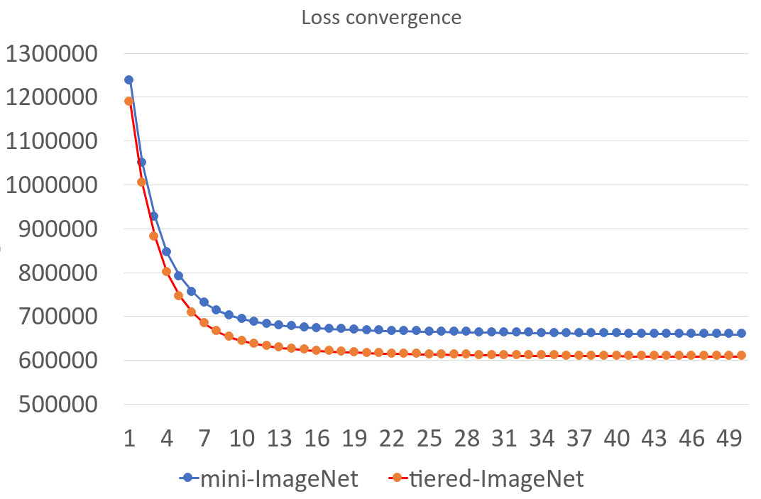
Figure 3: The loss curve (mini-ImageNet, tiered-ImageNet).

5 Conclusions

In this paper, we have pointed out disadvantages of prototype-based methods and label propagation based methods for transductive FSL. To overcome these drawbacks, we have presented a unified framework combining the prototype-based methods and label propagation based methods within a single objective. Our protoLP inherits advantages of individual prototype refinement and label propagation steps while avoiding the disadvantages of the bias in estimation of prototypes and the fixed graph bias. Our protoLP performs well also under non-uniform class priors unlike Sinhorn-based methods. The protoLP works with different backbones and is a plug-and-play module for the inference step of FSL.

Acknowledgements.

HZ is supported by an Australian Government Research Training Program (RTP) Scholarship. PK is in part funded by CSIRO’s Machine Learning and Artificial Intelligence Future Science Platform (MLAI FSP) Spatiotemporal Activity.

Transductive Few-shot Learning with Prototype-based Label Propagation by Iterative Graph Refinement (Supplementary Material)

Hao Zhu^†,§,    Piotr Koniusz^{∗,§,†
†}Australian National University $\quad{}^{\S}$Data61$\varheartsuit$CSIRO
allenhaozhu@gmail.com,  firstname.lastname@anu.edu.au

Below are additional details regarding our model and experiments.

6 Datasets

mini-ImageNet.

This dataset vinyals2016matching_supp,ravi2017optimization_supp is widely used in few-shot classification maxexp_supp,simon2022noise_supp,yao_cvpr2022_supp,simon2022wacv_supp,hong_tmm_supp,zhang2022accv_supp,simon_cvpr2023_supp. It contains 100 randomly chosen classes from ImageNet russakovsky2015imagenet_supp. There are 64 training (base) classes, 16 validation (novel) classes, and 20 test (novel) classes among the 100 classes. There are 600 images in each class. We adopt the split provided in ravi2017optimization_supp.

tiered-ImageNet.

ImageNet with a hierarchical structure was used to create the tiered-ImageNet. Categories of classes are divided into 34 categories, each of which contains 351, 97, and 160 classes for training, validation, and testing, respectively. Please note the training and test classes are semantically disjoint. We follow the common split in chen2021eckpn_supp and 84 by 84px resolution.

CIFAR-FS.

This dataset has 100 classes, each with 600 examples in CIFAR-100 krizhevsky2009learning_supp, on which this dataset is based on. We use the 64 training, 16 validation, and 20 test classes provided by chen2019closer_supp.

CUB.

There are 200 classes, each representing a bird species, in this fine-grained dataset. Following the setting in chen2019closer_supp , we divide our classes into three groups: 100 training, 50 validation, and 50 testing classes.

7 Feature Extraction and Pre-processing

ResNet-12A

is the pre-trained backbone network used in wang2020instance_supp. For all of our transductive and semi-supervised experiments using this network, we adopt exactly the same pre-processing as wang2020instance_supp, which includes normalizing feature vectors by their $\ell_{2}$ norms.

WRN-28-10

is the pre-trained network used in mangla2020charting_supp and hu2020leveraging_supp. To provide fair comparisons with PT+MAP hu2020leveraging_supp, we adopt exactly the same pre-processing as hu2020leveraging_supp. In the all experiments, we apply the power transform and normalize feature vectors by their $\ell_{2}$ norms.

DenseNet

is the pre-trained network used in lichtenstein2020tafssl_supp and wang2019simpleshot_supp. To provide fair comparisons with TASFFL lichtenstein2020tafssl_supp, we adopt exactly the same pre-processing. In the all experiments, we decentre feature vectors by using the center in the training set and normalize decentred feature vectors by their $\ell_{2}$ norms.

MobilieNet

is the pre-trained network used in wang2019simpleshot_supp. To provide fair comparison with LaplacianShot ziko2020laplacian_supp, we adopt exactly the same pre-processing. In the all experiments, we follow the setting as same as other backbones.

8 Hyper-parameters

In Eq. (8), parameter $\lambda$ is in charge of regularizing the graph. For the balanced class setting, we simply set $\lambda=1$. For the unbalanced class setting, we set $\lambda=0.5$.

Hyper-parameter $\alpha$ is used to control updating prototypes ${\bm{C}}$ in Eq. (17). We empirically found that $\alpha$ basically does not impact the final result but the convergence speed. In this paper, we set it as 0.2 for all experiments.

9 Note on Fair Comparisons

During our experimental studies, we noticed the importance of fair comparisons by ensuring the common testbed. Below we talk about common issues.

• Some comparisons use different networks. In some papers, ResNet-18 is compared directly with other methods using ResNet-12. In Table 1 (our main paper), we show that ResNet-18 has some advantages over ResNet-12 in some cases.

• Methods are mainly compared under the class-balanced prior. For ease of understanding, transductive FSL evolves directly from the setting of inductive FSL. Class-balanced queries are not an issue for inductive FSL because these methods treat queries one-by-one and ignore the class distribution of queries. However, the same setting in transductive setting introduces class-balanced prior. Many approaches over the last few years have focused on how to exploit this prior. We argue that this prior is unreasonable for transductive FSL, since it is rare for queries to follow a uniform class distribution. We can see the power of optimal transport under this prior i numerous works zhu2022ease_supp,hu2020leveraging_supp,lazarou2021iterative_supp. We can also see that this technique has the negative effect for queries that do not conform to the uniform class prior (e.g., PT-MAP hu2020leveraging_supp drop 17% in mini-ImageNet under the unbalanced setting). Without the optimal transport, these methods also loose performance in the balanced setting.

We hope that bringing attention to these evaluation issues will help researchers avoid following the unrealistic settings and move toward fairer evaluation protocols and models. We encourage the community to compare different methods with under the same testbed.

10 The motivation of Parameterized Label Prediction

From a theoretical point of view, if we do not use parameterized label prediction, we need to optimize:

$$\min_{\widetilde{{\bm{Y}}}}\frac{1}{2}\lVert\widetilde{{\bm{Y}}}_{L}-{\bm{Y}}_{L}\rVert_{F}^{2}+\frac{\lambda}{2}\operatorname{Tr}(\widetilde{{\bm{Y}}}^{\top}\left(\bm{I}-\lambda\bm{Z}\bm{\Lambda}^{-1}{\bm{Z}}^{\top}\right)\widetilde{{\bm{Y}}}).$$ (19)

The closed form solution is $\left(\bm{I}-\lambda{\bm{Z}}\bm{\Lambda}^{-1}{\bm{Z}}^{\top}\right)^{-1}{\bm{Y}}$. The computational complexity of the inverse matrix is $n^{3}$. and the $rank({\bm{Z}}\bm{\Lambda}^{-1}{\bm{Z}}^{\top})\!=\!5$ (for 5-way problem). Thus we can use linear function ${\bm{A}}$ to do propagation on ${\bm{Y}}$ and reduce computational complexity from $n^{3}$ to $c^{3}$ where $n\!\gg\!c$. Projection to low-dimensional space limits the number of unnecessary parameters. Experiments in Table 10 confirm the parameterized LP works better.

Table 10: Test accuracy on standard LP and parameterized LP setting (ResNet-12 backbone).

	mini-ImageNet		tiered-ImageNet		CUB
Methods (ResNet-18)	1-shot	5-shot	1-shot	5-shot	1-shot	5-shot
Ours (non-paramerized)	69.41	79.52	83.60	88.56	88.50	91.70
Ours (parameterized)	70.04	79.80	84.04	88.72	88.85	91.93

11 Inference Time

Table 11 provides the average inference time (1$\times$ AMD 3600 CPU) for the 1- and 5-shot tasks on mini-ImageNet (ResNet-12 and WRN-28-10).

Table 11: Average inference time (in seconds) for the 1-shot and 5-shot tasks in mini-ImageNet dataset with different backbones.

Backbone	ResNet-12		WRN-28-10
Shot	1	5	1	5
iLPC lazarou2021iterative_supp	4.5e-2	5.6e-2	5.5e-2	7.0e-2
ICI wang2020instance_supp	3.4e-2	4.2e-2	4.1e-2	5.2e-2
protoLP	4.7e-3	5.8e-3	6.2e-3	6.8e-3

ieee_fullname latex

References

- [1] Yassir Bendou, Yuqing Hu, Raphael Lafargue, Giulia Lioi, Bastien Pasdeloup, Stéphane Pateux, and Vincent Gripon. Easy—ensemble augmented-shot-y-shaped learning: State-of-the-art few-shot classification with simple components. Journal of Imaging, 8(7):179, 2022.
- [2] Malik Boudiaf, Imtiaz Ziko, Jérôme Rony, Jose Dolz, Pablo Piantanida, and Ismail Ben Ayed. Information maximization for few-shot learning. Advances in Neural Information Processing Systems, 33, 2020.
- [3] Chaofan Chen, Xiaoshan Yang, Changsheng Xu, Xuhui Huang, and Zhe Ma. Eckpn: Explicit class knowledge propagation network for transductive few-shot learning. In Proceedings of the IEEE/CVF Conference on Computer Vision and Pattern Recognition, pages 6596–6605, 2021.
- [4] Wei-Yu Chen, Yen-Cheng Liu, Zsolt Kira, Yu-Chiang Frank Wang, and Jia-Bin Huang. A closer look at few-shot classification. In International Conference on Learning Representations, 2019.
- [5] Marco Cuturi. Sinkhorn distances: Lightspeed computation of optimal transport. Advances in neural information processing systems, 26:2292–2300, 2013.
- [6] Guneet Singh Dhillon, Pratik Chaudhari, Avinash Ravichandran, and Stefano Soatto. A baseline for few-shot image classification. In International Conference on Learning Representations, 2020.
- [7] Li Fei-Fei, Rob Fergus, and Pietro Perona. One-shot learning of object categories. IEEE transactions on pattern analysis and machine intelligence, 28(4):594–611, 2006.
- [8] Chelsea Finn, Pieter Abbeel, and Sergey Levine. Model-agnostic meta-learning for fast adaptation of deep networks. In International Conference on Machine Learning, pages 1126–1135. PMLR, 2017.
- [9] Spyros Gidaris and Nikos Komodakis. Generating classification weights with gnn denoising autoencoders for few-shot learning. In Proceedings of the IEEE/CVF Conference on Computer Vision and Pattern Recognition, pages 21–30, 2019.
- [10] Jie Hong, Pengfei Fang, Weihao Li, Tong Zhang, Christian Simon, Mehrtash Harandi, and Lars Petersson. Reinforced attention for few-shot learning and beyond. In Proceedings of the IEEE/CVF Conference on Computer Vision and Pattern Recognition, pages 913–923, 2021.
- [11] Ruibing Hou, Hong Chang, Bingpeng Ma, Shiguang Shan, and Xilin Chen. Cross attention network for few-shot classification. Advances in Neural Information Processing Systems, 32, 2019.
- [12] Andrew G Howard, Menglong Zhu, Bo Chen, Dmitry Kalenichenko, Weijun Wang, Tobias Weyand, Marco Andreetto, and Hartwig Adam. Mobilenets: Efficient convolutional neural networks for mobile vision applications. arXiv preprint arXiv:1704.04861, 2017.
- [13] Shell Xu Hu, Pablo Garcia Moreno, Yang Xiao, Xi Shen, Guillaume Obozinski, Neil Lawrence, and Andreas Damianou. Empirical bayes transductive meta-learning with synthetic gradients. In International Conference on Learning Representations, 2020.
- [14] Yuqing Hu, Vincent Gripon, and Stéphane Pateux. Leveraging the feature distribution in transfer-based few-shot learning. In Artificial Neural Networks and Machine Learning–ICANN 2021: 30th International Conference on Artificial Neural Networks, Bratislava, Slovakia, September 14–17, 2021, Proceedings, Part II 30, pages 487–499. Springer, 2021.
- [15] Dahyun Kang, Piotr Koniusz, Minsu Cho, and Naila Murray. Distilling self-supervised vision transformers for weakly-supervised few-shot classification & segmentation. In Proceedings of the IEEE/CVF Conference on Computer Vision and Pattern Recognition, 2023.
- [16] Jongmin Kim, Taesup Kim, Sungwoong Kim, and Chang D Yoo. Edge-labeling graph neural network for few-shot learning. In Proceedings of the IEEE/CVF Conference on Computer Vision and Pattern Recognition, pages 11–20, 2019.
- [17] Philip A Knight. The sinkhorn–knopp algorithm: convergence and applications. SIAM Journal on Matrix Analysis and Applications, 30(1):261–275, 2008.
- [18] Piotr Koniusz and Krystian Mikolajczyk. Soft assignment of visual words as linear coordinate coding and optimisation of its reconstruction error. In 18th IEEE International Conference on Image Processing, 2011.
- [19] Piotr Koniusz and Hongguang Zhang. Power normalizations in fine-grained image, few-shot image and graph classification. IEEE Trans. Pattern Anal. Mach. Intell., 44(2):591–609, 2022.
- [20] Alex Krizhevsky, Geoffrey Hinton, et al. Learning multiple layers of features from tiny images. 2009.
- [21] Seong Min Kye, Hae Beom Lee, Hoirin Kim, and Sung Ju Hwang. Meta-learned confidence for few-shot learning. arXiv preprint arXiv:2002.12017, 2020.
- [22] Michalis Lazarou, Tania Stathaki, and Yannis Avrithis. Iterative label cleaning for transductive and semi-supervised few-shot learning. In Proceedings of the IEEE/CVF International Conference on Computer Vision, pages 8751–8760, 2021.
- [23] Yann LeCun, Yoshua Bengio, and Geoffrey Hinton. Deep learning. nature, 521(7553):436–444, 2015.
- [24] Kwonjoon Lee, Subhransu Maji, Avinash Ravichandran, and Stefano Soatto. Meta-learning with differentiable convex optimization. In Proceedings of the IEEE/CVF Conference on Computer Vision and Pattern Recognition, pages 10657–10665, 2019.
- [25] Xinzhe Li, Qianru Sun, Yaoyao Liu, Shibao Zheng, Qin Zhou, Tat-Seng Chua, and Bernt Schiele. Learning to self-train for semi-supervised few-shot classification (6 2019). In Advances in Neural Information Processing Systems: 33rd Conference on Neural Information Processing Systems (NeurIPS 2019), Vancouver, Canada, December, volume 8, pages 1–11, 1906.
- [26] Moshe Lichtenstein, Prasanna Sattigeri, Rogerio Feris, Raja Giryes, and Leonid Karlinsky. Tafssl: Task-adaptive feature sub-space learning for few-shot classification. In European Conference on Computer Vision, pages 522–539. Springer, 2020.
- [27] Jinlu Liu, Liang Song, and Yongqiang Qin. Prototype rectification for few-shot learning. In European Conference on Computer Vision, pages 741–756. Springer, 2020.
- [28] Wei Liu, Junfeng He, and Shih-Fu Chang. Large graph construction for scalable semi-supervised learning. In Proceedings of the 27th International Conference on International Conference on Machine Learning, pages 679–686, 2010.
- [29] Yanbin Liu, Juho Lee, Minseop Park, Saehoon Kim, Eunho Yang, Sungju Hwang, and Yi Yang. Learning to propagate labels: Transductive propagation network for few-shot learning. In International Conference on Learning Representations, 2019.
- [30] Changsheng Lu and Piotr Koniusz. Few-shot keypoint detection with uncertainty learning for unseen species. In Proceedings of the IEEE/CVF Conference on Computer Vision and Pattern Recognition, 2022.
- [31] Puneet Mangla, Nupur Kumari, Abhishek Sinha, Mayank Singh, Balaji Krishnamurthy, and Vineeth N Balasubramanian. Charting the right manifold: Manifold mixup for few-shot learning. In Proceedings of the IEEE/CVF Winter Conference on Applications of Computer Vision, pages 2218–2227, 2020.
- [32] Nikhil Mishra, Mostafa Rohaninejad, Xi Chen, and Pieter Abbeel. A simple neural attentive meta-learner. arXiv preprint arXiv:1707.03141, 2017.
- [33] Boris N Oreshkin, Pau Rodriguez, and Alexandre Lacoste. Tadam: Task dependent adaptive metric for improved few-shot learning. arXiv preprint arXiv:1805.10123, 2018.
- [34] Guodong Qi, Huimin Yu, Zhaohui Lu, and Shuzhao Li. Transductive few-shot classification on the oblique manifold. In Proceedings of the IEEE/CVF International Conference on Computer Vision, pages 8412–8422, 2021.
- [35] Limeng Qiao, Yemin Shi, Jia Li, Yaowei Wang, Tiejun Huang, and Yonghong Tian. Transductive episodic-wise adaptive metric for few-shot learning. In Proceedings of the IEEE/CVF International Conference on Computer Vision, pages 3603–3612, 2019.
- [36] Sachin Ravi and Hugo Larochelle. Optimization as a model for few-shot learning. In International Conference on Learning Representations, 2017.
- [37] Mengye Ren, Sachin Ravi, Eleni Triantafillou, Jake Snell, Kevin Swersky, Josh B. Tenenbaum, Hugo Larochelle, and Richard S. Zemel. Meta-learning for semi-supervised few-shot classification. In International Conference on Learning Representations, 2018.
- [38] Pau Rodríguez, Issam Laradji, Alexandre Drouin, and Alexandre Lacoste. Embedding propagation: Smoother manifold for few-shot classification. In European Conference on Computer Vision, pages 121–138. Springer, 2020.
- [39] Andrei A. Rusu, Dushyant Rao, Jakub Sygnowski, Oriol Vinyals, Razvan Pascanu, Simon Osindero, and Raia Hadsell. Meta-learning with latent embedding optimization. In International Conference on Learning Representations, 2019.
- [40] Victor Garcia Satorras and Joan Bruna Estrach. Few-shot learning with graph neural networks. In International Conference on Learning Representations, 2018.
- [41] Xi Shen, Yang Xiao, Shell Hu, Othman Sbai, and Mathieu Aubry. Re-ranking for image retrieval and transductive few-shot classification. Advances in Neural Information Processing Systems, 34, 2021.
- [42] Christian Simon, Piotr Koniusz, and Mehrtash Harandi. Meta-learning for multi-label few-shot classification. In Proceedings of the IEEE/CVF Winter Conference on Applications of Computer Vision, 2022.
- [43] Christian Simon, Piotr Koniusz, Richard Nock, and Mehrtash Harandi. Adaptive subspaces for few-shot learning. In Proceedings of the IEEE/CVF Conference on Computer Vision and Pattern Recognition, pages 4136–4145, 2020.
- [44] Jake Snell, Kevin Swersky, and Richard Zemel. Prototypical networks for few-shot learning. Advances in neural information processing systems, 30, 2017.
- [45] Flood Sung, Yongxin Yang, Li Zhang, Tao Xiang, Philip HS Torr, and Timothy M Hospedales. Learning to compare: Relation network for few-shot learning. In Proceedings of the IEEE conference on computer vision and pattern recognition, pages 1199–1208, 2018.
- [46] Olivier Veilleux, Malik Boudiaf, Pablo Piantanida, and Ismail Ben Ayed. Realistic evaluation of transductive few-shot learning. Advances in Neural Information Processing Systems, 34:9290–9302, 2021.
- [47] Oriol Vinyals, Charles Blundell, Timothy Lillicrap, Daan Wierstra, et al. Matching networks for one shot learning. Advances in neural information processing systems, 29, 2016.
- [48] Lei Wang and Piotr Koniusz. Temporal-viewpoint transportation plan for skeletal few-shot action recognition. In Asian Conference on Computer Vision, 2022.
- [49] Lei Wang and Piotr Koniusz. Uncertainty-dtw for time series and sequences. In European Conference on Computer Vision, 2022.
- [50] Yan Wang, Wei-Lun Chao, Kilian Q Weinberger, and Laurens van der Maaten. Simpleshot: Revisiting nearest-neighbor classification for few-shot learning. arXiv preprint arXiv:1911.04623, 2019.
- [51] Yikai Wang, Chengming Xu, Chen Liu, Li Zhang, and Yanwei Fu. Instance credibility inference for few-shot learning. In Proceedings of the IEEE/CVF Conference on Computer Vision and Pattern Recognition, pages 12836–12845, 2020.
- [52] Peter Welinder, Steve Branson, Takeshi Mita, Catherine Wah, Florian Schroff, Serge Belongie, and Pietro Perona. Caltech-ucsd birds 200. 2010.
- [53] Weijian Xu, yifan xu, Huaijin Wang, and Zhuowen Tu. Attentional constellation nets for few-shot learning. In International Conference on Learning Representations, 2021.
- [54] Han-Jia Ye, Hexiang Hu, De-Chuan Zhan, and Fei Sha. Few-shot learning via embedding adaptation with set-to-set functions. In Proceedings of the IEEE/CVF Conference on Computer Vision and Pattern Recognition, pages 8808–8817, 2020.
- [55] Hongguang Zhang, Philip H. S. Torr, and Piotr Koniusz. Improving few-shot learning by spatially-aware matching and crosstransformer. In Asian Conference on Computer Vision, 2022.
- [56] Shan Zhang, Dawei Luo, Lei Wang, and Piotr Koniusz. Few-shot object detection by second-order pooling. In Asian Conference on Computer Vision, 2020.
- [57] Shan Zhang, Naila Murray, Lei Wang, and Piotr Koniusz. Time-reversed diffusion tensor transformer: A new tenet of few-shot object detection. In European Conference on Computer Vision, 2022.
- [58] Shan Zhang, Lei Wang, Naila Murray, and Piotr Koniusz. Kernelized few-shot object detection with efficient integral aggregation. In Proceedings of the IEEE/CVF Conference on Computer Vision and Pattern Recognition, 2022.
- [59] Dengyong Zhou, Olivier Bousquet, Thomas Lal, Jason Weston, and Bernhard Schölkopf. Learning with local and global consistency. Advances in neural information processing systems, 16, 2003.
- [60] Hao Zhu and Piotr Koniusz. EASE: Unsupervised discriminant subspace learning for transductive few-shot learning. In Proceedings of the IEEE/CVF Conference on Computer Vision and Pattern Recognition, pages 9078–9088, 2022.
- [61] Imtiaz Ziko, Jose Dolz, Eric Granger, and Ismail Ben Ayed. Laplacian regularized few-shot learning. In International Conference on Machine Learning, pages 11660–11670. PMLR, 2020.