Learning Partial Correlation based Deep Visual Representation for Image Classification

Abstract

Visual representation based on covariance matrix has demonstrates its efficacy for image classification by characterising the pairwise correlation of different channels in convolutional feature maps. However, pairwise correlation will become misleading once there is another channel correlating with both channels of interest, resulting in the “confounding” effect. For this case, “partial correlation” which removes the confounding effect shall be estimated instead. Nevertheless, reliably estimating partial correlation requires to solve a symmetric positive definite matrix optimisation, known as sparse inverse covariance estimation (SICE). How to incorporate this process into CNN remains an open issue. In this work, we formulate SICE as a novel structured layer of CNN. To ensure end-to-end trainability, we develop an iterative method to solve the above matrix optimisation during forward and backward propagation steps. Our work obtains a partial correlation based deep visual representation and mitigates the small sample problem often encountered by covariance matrix estimation in CNN. Computationally, our model can be effectively trained with GPU and works well with a large number of channels of advanced CNNs. Experiments show the efficacy and superior classification performance of our deep visual representation compared to covariance matrix based counterparts.

1 Introduction

Learning effective visual representation is a central issue in computer vision. In the past two decades, describing images with local features and pooling them to a global representation has shown promising performance. As one of the pooling methods, covariance matrix based pooling has attracted much attention due to its exploitation of second-order correlation information of features. A variety of tasks such as fine-grained image classification [27], image segmentation [16], generic image classification [24, 26, 34], image set classification [44], action recognition [18], few-shot classification [50] and few-shot detection [52, 54, 53] have benefited from the covariance matrix based representation. A few pioneering works have integrated covariance matrix as a pooling method within convolutional neural networks (CNN) and investigated associated issues such as matrix function backpropagation [16], matrix normalisation [28, 23, 38], compact matrix estimation [11, 49] and kernel based extension [9]. The above works further improved visual representations based on covariance matrix.

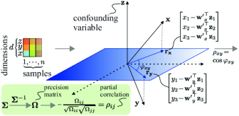
Figure 1: Understanding the partial correlation (a 3D toy case). Unlike the ordinary covariance (pairwise correlation of say $\mathbf{x}$ and $\mathbf{y}$ corresponding to channels), partial correlation between variables $\mathbf{x}$ and $\mathbf{y}$ removes the influence of the confounding variable $\mathbf{z}$. Let the number of samples $n\!=\!3$ and channels $d\!=\!3$. For the 3D case, $\mathbf{x}$ and $\mathbf{y}$ are projected onto a plane perpendicular to $\mathbf{z}$. Then $\rho_{xy}\!=\!\cos{\varphi_{xy}}$ (and $\rho_{xz}$ and $\rho_{yz}$ can be computed by analogy). Projected “residuals” $\mathbf{r}_{\mathbf{x}}$ and $\mathbf{r}_{\mathbf{y}}$ are computed as indicated in the plot, ${\mathbf{w}^{\prime}\!}_{x}\!=\!\operatorname*{arg\,min}_{\mathbf{w}}\sum_{i=1}^{3}(x_{i}\!-\!\mathbf{w}_{x}^{\top}\mathbf{z}_{i})$ where $\mathbf{z}_{i}\!=\![z_{i},1]^{\top}$ (and ${\mathbf{w}^{\prime}\!}_{y}$ is computed by analogy). The green box: for $d\!>\!3$, the computation of partial correlation requires covariance inversion [7].

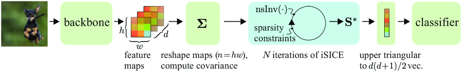
Figure 2: Proposed iterative sparse inverse covariance estimation (iSICE) method in a CNN pipeline.

Despite the above progress, covariance matrix merely measures the pairwise correlation (more accurately, covariance) of two variables without taking any other variables into account. This can be easily verified because its $(i,j)$-th entry solely depends on the $i$-th and $j$-th variables on a sample set. In Statistics, it is known that such a pairwise correlation will give misleading results once a third variable is correlated with both variables of interest due to the “confounding” effect. For this situation, the partial correlation is the right measure to use. It regresses out the effects of other variables from the two variables and then calculates the correlation of their residuals instead. Partial correlation can be conveniently obtained by computing inverse covariance matrix, also known as the precision matrix [7] in the statistical community. Figure 1 illustrates the geometrical interpretation of partial correlation.

The above observation motivates us to investigate a visual representation for image classification based on the inverse covariance matrix. After all, it has better theoretical support on characterising the essential relationship of variables (e.g., the channels in a convolutional feature map) when other variables are present. Note that inverse covariance matrix can be used for many vision tasks but in this paper, we investigate it from the perspective of image classification. Nevertheless, reliably estimating inverse covariance matrix from the local descriptors of a CNN feature map is a challenging task. This is primarily due to the small spatial size of the feature map, i.e., sample size, and a higher number of channels, i.e., feature dimensions, and this issue becomes more pronounced for advanced CNN models. An unreliable estimate of inverse covariance matrix will critically affect its effectiveness as a visual representation. One might argue that by increasing the size of input images or using a dimension reduction layer to reduce the number of feature channels, such an issue could be resolved. In this paper, we investigate this issue from the perspective of robust precision matrix estimation.

To achieve our goal, we explore the use of sparsity prior for inverse covariance matrix estimation in the literature. Specifically, the general principle of “bet on sparsity” [12] is adopted in estimating the structure of high-dimensional data, and this leads to an established technique called sparse inverse covariance estimation (SICE) [10]. It solves an optimisation in the space of symmetric and positive definite (SPD) matrix to estimate the inverse covariance matrix by imposing the sparsity prior on its entries. SICE is designed to handle small sample problem and it is known for its excellent effectiveness to that end [10]. An initial attempt to apply SICE for visual representation is based on handcrafted or pre-extracted features of small size and an off-the-shelf SICE solver, and it does not have the ability to backpropagate through SICE due to optimisation of the SPD matrix with the imposed non-smooth sparsity term [51].

Our work is the first one that truly integrates SICE into CNN for end-to-end training. Clearly, such an integration will fully take advantage of the feature learning capability of CNN and the partial correlation offered by inverse covariance matrix. On the other hand, realising such an integration is not trivial. Unlike covariance matrix, which is obtained by simple arithmetic operations, SICE is obtained by solving an SPD matrix based optimisation. How to incorporate this optimisation process into CNN as a layer is an issue. Furthermore, this SICE optimisation needs to be solved for each training image during both forward and backward phases to generate a visual representation. Directly solving this optimisation within CNN will not be practical even for a medium-sized SICE problem.

To efficiently integrate SICE into CNN, we propose a fast end-to-end training method for SICE by taking inspiration from Newton-Schulz iteration [14]. Our method solves the SICE optimisation with a smooth convex cost function by re-parameterising the non-smooth term in the original SICE cost function (see Eq. (1)), and it can therefore be optimised with standard optimisation techniques such as gradient descend. Furthermore, we effectively enforce the SPD constraint during optimisation so that the obtained SICE solution remains SPD as desired. Figure 2 shows our “Iterative Sparse Inverse Covariance Estimation (iSICE)”. In contrast to SICE, iSICE works with end-to-end trainable deep learning models. Our iSICE involves simple matrix arithmetic operations fully compatible with GPU. It can approximately solve large SICE problems within CNN efficiently.

Our main contributions are summarised as follows.

1. To more precisely characterise the relationship of features for visual representation, this paper proposes to integrate sparse inverse covariance estimation (SICE) process into CNNs as a novel layer. To achieve this, we develop a method based on Newton-Schulz iteration and box constraints for $\ell_{1}$ penalty to solve the SICE optimisation with CNN and maintain the end-to-end training efficiency. To the best of our knowledge, our iSICE is the first end-to-end SICE solution for CNN.

2. Our iSICE method requires a minimal change of network architecture. Therefore, it can readily be integrated with existing works to replace those using deep network models to learn covariance matrix based visual representation. The iSICE is fully compatible with GPU and can be easily implemented with modern deep learning libraries.

3. As the objective of SICE is a combination of $\log\det$ term (may change rapidly) and sparsity (changes slowly), achieving the balance between both terms during optimisation by the gradient descent is hard. To this end, we propose a minor contribution: a simple modulating network whose goal is to adapt on-the-fly learning rate and sparsity penalty.

Experiments on multiple image classification datasets show the effectiveness of our proposed iSICE method.

2 Related work

Since the advent of covariance representation methods in deep learning [27, 11], reliable estimation of the covariance matrix from a CNN feature map remains an issue. The issue is due to the small spatial size of feature map (corresponding to the number of samples) and the higher number of feature channels (corresponding to the feature dimensions), which could cause unreliable estimation and even matrix singularity due to the so-called “curse of dimensionality”. Existing works either append a small positive constant to the diagonals of covariance matrix [27] or use matrix normalisation operation [16, 28, 24] to handle this issue. Matrix normalisation approaches mitigate unbalanced spectrum represented by eigenvalues of covariance matrix [19, 24, 25, 20, 55]. Different from the existing methods, in this paper, we approach the reliable covariance estimation problem in CNN from a perspective of partial correlations that can be efficiently captured by the inverse of covariance matrix, also known as the precision matrix [7], when a large number of samples is available for estimation.

Covariance representation strives to capture the underlying structure of CNN feature channels. In the literature of knowledge representation [22], it is recommended to leverage prior knowledge to improve a learning task when sufficient data is not available. Thus, prior knowledge can be used to improve the estimation of underlying structure of high-dimensional data captured by covariance representation. One common prior knowledge is “structure sparsity” which leads to the sparse inverse covariance matrix in the literature of statistical machine learning [10, 15].

Structure sparsity cannot be readily applied to covariance representation as it requires the access to partial correlation between feature components. A covariance matrix captures pairwise correlation of feature components without taking into account the confounding effect of remaining components. Therefore, it is unlikely that the covariance matrix will be sparse by nature. To obtain partial correlation, SICE moves from covariance matrix to its inverse. An inverse covariance matrix captures partial correlation between feature components by regressing out the effects of other variables [15]. Once other variables are factored out, structure sparsity can be effectively enforced in SICE. In a recent work [51], SICE-based visual representation has been applied to image classification with handcrafted and pre-extracted features of small size. However, SICE has never been integrated into CNN for end-to-end training with the goal of adapting to such a representation. The existing solvers for computing SICE also have limited GPU support [10, 8]. Thus, we propose an end-to-end trainable iterative method for solving SICE optimisation with CNNs.

3 Proposed method

In this section, we begin by discussing the background of SICE. Then we discuss how it can be estimated from CNN feature descriptors. Finally, we describe our proposed method which is trainable end-to-end with a CNN.

3.1 The basic idea of SICE

As a representation, the covariance matrix captures the underlying structure of a feature set. It uses a covariance matrix estimated from samples to capture this structure. Sparse inverse covariance estimation (SICE) focuses on the following two issues: (1) instability or singularity of sample-based covariance matrix estimated from a small number of high-dimensional feature vectors. This situation makes it less effective in capturing the underlying structure of data. As an example, in this case the smaller and larger eigenvalues of the estimated covariance matrix become poorly estimated. Thus, a suitable regularisation (a prior) is needed during the estimation to mitigate the bias of our estimator; (2) rigid estimation of covariance matrix for high-dimensional feature vectors is not always appropriate as the high-dimensional data usually presents a complex structure. If there is prior knowledge available, it should be used to improve the covariance estimation from a small number of samples.

In terms of prior knowledge of high-dimensional data, structure sparsity [15] and the “bet on sparsity” principle [12] are the two common priors used in the literature. Suppose that we have a probabilistic graphical model, where each node corresponds to a feature and the statistical dependence between two nodes is expressed with an edge linking two nodes. Structure sparsity would specify how sparse such a graph is, e.g., how many edges are presented in this graph. More generally, even if there is no clear prior knowledge on structure sparsity available, the “bet on sparsity” principle can still be applied to estimate the structure of the graph by imposing a sparsity prior. Its rationality is as follows. If the graph is indeed sparse, SICE will estimate its underlying structure with a correct prior, and if the graph is dense, it will not estimate the underlying structure accurately with such a prior. However, in the latter case, we will not lose much because we have known that we do not have enough sample to estimate the dense structure. The “bet on sparsity” principle has been widely adopted in high-dimensional data analysis, and also demonstrated its efficacy on covariance matrix based visual representation estimated from handcrafted or pre-extracted CNN features [51].

SICE strives to improve the covariance estimation with the use of prior knowledge. To incorporate prior knowledge, SICE switches to the inverse of covariance matrix from covariance matrix. In principle, the covariance matrix captures the apparent pairwise correlation between feature components, i.e., indirect correlation. In comparison, the inverse of covariance matrix is able to characterise the direct (i.e. partial) correlation between two feature components by regressing out the remaining features. Using the inverse covariance matrix not only helps to interpret the essential relationship between two features, but also allows the convenient incorporation of the sparsity prior.

3.2 Our SICE estimation with CNN

Suppose, we have the sample-based covariance matrix $\mathbf{\Sigma}$ computed from a set of CNN local descriptors presented in a convolutional feature map. Let $\mathbf{S}$ denote the corresponding sparse inverse covariance matrix. The off-diagonal entries of $\mathbf{S}$ capture the direct correlation between different descriptor components. They are zero if two components are independent under the removed influence of confounding variables. In the literature [10], the estimation of $\mathbf{S}$ has been effectively resolved by the maximization of a penalised log-likelihood of data with an SPD constraint on $\mathbf{S}$ and the sparsity prior to induce sparse graph connectivity. The optimal solution of the above problem is known as SICE.

To obtain reliable and faithful SICE, the term $\lVert\mathbf{S}\rVert_{1}$ imposes the structure sparsity on $\mathbf{S}$. $\lambda$ controls the trade-off between the amount of sparsity and the log-likelihood estimation. The problem in Eq. (1) is convex and can be solved by the off-the-shelf packages such as GLASSO [10] and CVXPY [8]. However, the objective is non-smooth due to the $\ell_{1}$ penalty. The above optimisation packages cannot be used with CNN layers to conduct training with backpropagation. A recent extension of CVXPY called CVXPYLAYERS [1] provides differentiable optimisation layers. However, based on our investigation, it has the following issues: (1) it cannot efficiently solve large SICE problems, i.e., of size $128\!\times\!128$ or higher; (2) it relies on multiple CPU based libraries including CVXPY to solve the optimisation problem and obtain gradients for backpropagation. This greatly limits its efficiency due to the lack of GPU support. The above limitations motivate us to develop an SICE method suitable for end-to-end training with GPU.

3.3 Proposed end-to-end trainable SICE method

Let $J$ be the objective function of Eq. (1). $J$ can be optimised by taking the gradient with respect to $\mathbf{S}$ as follows:

$$\frac{\partial J}{\partial\mathbf{S}} =\frac{\partial}{\partial\mathbf{S}}\log\,\det(\mathbf{S})-\frac{\partial}{\partial\mathbf{S}}\mathrm{trace}(\mathbf{\Sigma S})-\lambda\frac{\partial}{\partial\mathbf{S}}\lVert\mathbf{S}\rVert_{1}$$

$$=\mathbf{S}^{-1}-\mathbf{\Sigma}-\lambda\Big{(}\frac{\partial}{\partial\mathbf{S}}\mathbf{S}^{+}-\frac{\partial}{\partial\mathbf{S}}\mathbf{S}^{-}\Big{)}$$

$$=\mathbf{S}^{-1}-\mathbf{\Sigma}-\lambda\big{(}\mathrm{sign}(\mathbf{S}^{+})-\mathrm{sign}(\mathbf{S}^{-})\big{)},$$ (2)

where $\mathbf{S}^{+}\equiv\mathrm{max}(0,\mathbf{S})$ and $\mathbf{S}^{-}\equiv\mathrm{max}(0,-\mathbf{S})$ contain the positive and negative parts of $\mathbf{S}$, respectively. Eq. (2) can be optimised with the projected gradient descend which has the native backpropagation support on GPU and can take advantage of GPU parallel computing to improve their speed. Now we discuss how Eq. (2) can be effectively optimised using a few consecutive structured CNN layers.

The overview of our method is given in Fig. 2. From the left, we pass an input image to the backbone and process it till the last convolution layer. We obtain the feature map, i.e., $h\times w\times d$ tensor, where $h$ is the height, $w$ is the width, and $d$ is the number of channels. By reshaping the feature map to a set of $n$ vectors of length $d$, where $n=wh$ and stacking them as column vectors, we can create a $d\times n$ data matrix $\mathbf{X}$. A sample-based covariance matrix $\mathbf{\Sigma}$ estimated from $\mathbf{X}$ is defined as $\mathbf{\Sigma}\equiv\mathbf{X\bar{I}}\mathbf{X}^{\top}$, where $\mathbf{\bar{I}}=\frac{1}{n}(\mathbf{I}-\frac{1}{n}\mathbf{1}\mathbf{1}^{\top})$ performs centering of matrix $\mathbf{X}$, where $\mathbf{I}$ and $\mathbf{1}\mathbf{1}^{\top}$ are $n\times n$ dimensional identity matrix and matrix of all-ones, respectively. Below, we describe key steps of our method.

Estimation of precision matrix $\mathbf{S}_{0}\!=\!\mathbf{\Sigma}^{\prime-1}$. Newton-Schulz iteration is popular as it can approximate the matrix square root fast on GPU [23]. In contrast, during the estimation of $\mathbf{S}$, we use Newton-Schulz iteration [14] for a fast approximate inverse of matrix, which imposes a convergence condition $\lVert\mathbf{\Sigma}-\mathbf{I}\rVert_{2}\!<\!1$ on Algorithm 1. Thus, we normalise $\mathbf{\Sigma}$ by its trace and use the trace-normalised $\mathbf{\Sigma}^{\prime}\!=\mathbf{\Sigma}/\mathrm{trace}(\mathbf{\Sigma})$. Then, the square of the inverse square root $\mathbf{Q}$ is post-normalized by the trace to reverse it, i.e., $\mathbf{\Sigma}^{-1}\!=\!\mathbf{Q}\mathbf{Q}^{\top}/\mathrm{trace}(\mathbf{\Sigma})$.

As Eq. (2) has to start with an initial $\mathbf{S}_{0}$, if $\mathbf{\Sigma}^{\prime}$ is invertible, Alg. 1 approximates its inverse. Although it is an approximation, we denote it in Alg. 1 as $\mathbf{\Sigma}^{-1}$ for brevity.

Algorithm 1 Matrix inverse by Newton-Schulz iterations, named $\text{nsInv}(\cdot)$. It is used to compute “Precision $\mathbf{\Omega}$” and is also used by Alg. 2, whereas $\mathbf{Y}_{N_{s}}$ (line 4) gives iSQRT.

Input: Covariance matrix $\mathbf{\Sigma}$, number of iterations $N_{s}$.
Output: Inverse covariance matrix $\mathbf{\Sigma}^{-1}$.

1:  $\mathbf{Y}_{0}\!=\!\mathbf{\Sigma}^{\prime}\!=\!\mathbf{\Sigma}$/trace($\mathbf{\Sigma}$), $\mathbf{Z}_{0}\!=\!\mathbf{{I}}$

2:  for $i=1$ to $N_{s}$ do

3:     $\mathbf{P}\!=\!\frac{1}{2}(3\mathbf{I}-\mathbf{Z}_{i-1}\mathbf{Y}_{i-1})$ 

4:     $\mathbf{Y}_{i}=\mathbf{Y}_{i-1}\mathbf{P}\;\;\;\text{and}\;\;\;\mathbf{Z}_{i}=\mathbf{P}\mathbf{Z}_{i-1}$ 

5:  end for

6:  $\mathbf{Q}=\mathbf{Z}_{N_{s}}$

7:  $\mathbf{\Sigma}^{-1}=\mathbf{Q}\mathbf{Q}^{\top}/\mathrm{trace}(\mathbf{\Sigma})$ {Inverse covariance matrix}

Estimation of sparse inverse covariance $\mathbf{S}$. Given the result obtained in the last step, $\mathbf{S}_{0}$, we start iterations of iSICE by applying the projected gradient descend (PGD) to the gradient of SICE (Eq. (1)), given in Eq. (2).

Following methodology of optimisation by imposing box constraints (e.g., see an intuitive example by Schiele et al. [35]), we separate $\mathbf{S}$ into its positive and negative parts:

$$\mathbf{S}_{i}^{+}=\max(0,\mathbf{S}_{i-1})\quad\text{and}\quad\mathbf{S}_{i}^{-}=\max(0,-\mathbf{S}_{i-1}),$$ (3)

and apply the PGD step to each of them separately.

In such a case, the sparsity constraint imposed by the $\ell_{1}$ norm simplifies, i.e., the gradient of $\lambda\mathbf{S}^{+}$ can be assumed $\lambda$ and the gradient of $-\lambda\mathbf{S}^{-}$ can be also assumed $\lambda$. Thus, we firstly rewrite Eq. (2) into two parts:

$$\nabla\mathbf{S}_{i}^{+}=\mathbf{S}_{i-1}-\mathbf{\Sigma}-\lambda\quad\text{and}\quad-\nabla\mathbf{S}_{i}^{-}=\mathbf{S}_{i-1}-\mathbf{\Sigma}+\lambda.$$ (4)

Then we take one PGD step to update $\mathbf{S}_{i}^{+}$ and $\mathbf{S}_{i}^{-}$:

$$\mathbf{S}_{i}^{+}:=\mathrm{\Pi}(\mathbf{S}_{i}^{+}-\eta\beta\nabla\mathbf{S}_{i}^{+})\quad\text{and}\quad\mathbf{S}_{i}^{-}:=\mathrm{\Pi}(\mathbf{S}_{i}^{-}-\eta\beta\nabla\mathbf{S}_{i}^{-}),$$ (5)

where $\Pi(\cdot)\equiv\mathrm{max}(0,\cdot)\equiv\mathrm{ReLU}(\cdot)$ is the gradient reprojection function of PGD into the feasible region of each box constraint (one for the non-negative $\mathbf{S}_{i}^{+}$, and one for non-positive $\mathbf{S}_{i}^{-}$). Constant $\eta>0$ is a desired learning rate, whereas $\beta>0$ controls the decay of learning rate.

Finally, we assemble the current estimate of $\mathbf{S}_{i}$ from $\mathbf{S}_{i}^{+}$ and $\mathbf{S}_{i}^{-}$:

$$\mathbf{S}_{i}=\text{Sym}(\mathbf{S}_{i}^{+}-\mathbf{S}_{i}^{-}),$$ (6)

where $\text{Sym}(\mathbf{M})\!=\!\frac{1}{2}(\mathbf{M}+\mathbf{M}^{\top})$ ensures the matrix $\mathbf{M}$ is symmetric (and the intermediate estimate of SICE).

Algorithm 2 starts with a dense precision matrix $\mathbf{S}_{0}$. If $N>0$, it loops over iterations $i=1,\cdots,N$, applying the above steps. For ease of tuning the learning rate $\eta$, the algorithm starts by the trace normalisation of $\mathbf{\Sigma}$ and it reverses the trace normalisation when it finishes. Otherwise, $\eta$ has to be scaled depending on the value of the largest eigenvalue of $\mathbf{\Sigma}$ which is somewhat impractical when running CNN end-to-end over multiple mini-batches.

Algorithm 2 Iterative sparse inverse covariance estimation (iSICE).

Input: Sample-based covariance matrix $\mathbf{\Sigma}$, sparsity constant $\lambda$, learning rate $\eta$, number of iterations N, small constant $\alpha$, i.e., $\alpha$ = 1e-9, regularisation parameter $\beta$.
Output: Sparse inverse covariance matrix $\mathbf{S}^{\prime}$.

1:  $\nabla_{2}\!=\!\mathbf{\Sigma}^{\prime}\!=\!\mathbf{\Sigma}$/trace($\mathbf{\Sigma}$) {Pre-normalisation using trace}

2:  $\mathbf{S}_{0}\!=\!\text{nsInv}(\mathbf{S}_{i-1}\!+\!\alpha\mathbf{I}$) {Fast approx. inverse (Alg. 1)}

3:  $\nabla_{1}\!=\!\mathbf{S}_{0}$

4:  for $i=1$ to $N$ do

5:     $\mathbf{S}_{i}^{+}\!=\mathrm{ReLU}(\mathbf{S}_{i-1})$ and $\mathbf{S}_{i}^{-}=\mathrm{ReLU}(-\mathbf{S}_{i-1})$

6:     if $i\neq 1$ 

7:        $\nabla_{1}\!=\!\text{nsInv}(\mathbf{S}_{i-1}\!+\!\alpha\mathbf{I}$) {Fast approx. inv. (Alg. 1)}

8:     end if

9:     $\nabla_{12}=\nabla_{1}-\nabla_{2}$ 

10:     $\beta=1-\frac{i-1}{\max(1,{N}-1)}$ {Decay the learning rate}

11:     $\mathbf{S}_{i}^{+}\!:=\mathrm{\Pi}\big{(}\mathbf{S}_{i}^{+}\!-\eta\beta(-\nabla_{12}+\lambda)\big{)}$

12:     $\mathbf{S}_{i}^{-}\!:=\mathrm{\Pi}\big{(}\mathbf{S}_{i}^{-}\!-\eta\beta(+\nabla_{12}+\lambda)\big{)}$

13:     $\mathbf{S}_{i}=\text{Sym}(\mathbf{S}_{i}^{+}\!-\mathbf{S}_{i}^{-})$ 

14:  end for

15:  $\mathbf{S}^{*}=\mathbf{S}_{N}/{\mathrm{trace}(\mathbf{S}_{N})}$

As $\mathbf{S}^{*}$ is a symmetric matrix, we only take its upper-triangular entries (plus the diagonal entries) and process them by fully connected layers for classification purposes.

Algorithm 2 is implemented with modern deep learning library, PyTorch, to leverage the full GPU support and autograd package for optimisation. Due to the iterative nature of solving $\mathbf{S}$, we call our method iterative SICE (iSICE).

4 Experiments

Below, we first describe experimental dataset benchmarks and then discuss the implementation of our proposed method. Subsequently, we present our experimental results and ablation study on key hyper-parameters. Finally, we compare our proposed method with the existing methods.

4.1 Datasets, Metric, and Implementation

Datasets. We conduct experiments using one scene and five fine-grained image datasets: the MIT Indoor dataset [33], Airplane [32], Birds [42], Cars [21], DTD [5] and iNaturalist [40]. We also use ImageNet100 (a subset of ImageNet-1K dataset) proposed by Tian et al. [39] and mini-ImageNet [41]. We follow the widely used training and testing protocols of Bilinear CNN [27]. The details of datasets and protocols are provided in Appendix A.

Metric for evaluations. For evaluation of different methods, average classification accuracy is used. This metric is widely used in literature, e.g., [27, 23].

Implementation details. Our method is implemented using PyTorch 1.9. We use ImageNet-1K pre-trained backbones provided in Torchvision 0.13.0 library. Following the recent works [24, 23], the number of feature channels is reduced to 256 with $1\times 1$ convolution for efficiency and fair comparisons. All images are resized to $448\times 448$ and the training is conducted by randomly flipping them horizontally. We fine-tune all backbones for 50-100 epochs with AdamW optimiser [31] for an initial learning rate of 0.00012, and ConvNext-T CNN and Swin-T with an initial learning rate 0.00005. For all backbones, we decrease the learning rate by a factor of 10 at the 15th and 30th epochs. Depending on the dataset and backbones, our fine-tuning process lasts for about 3-8 hours on four P100 GPUs. For ImageNet100, ResNet-50 was trained for 100 epochs with the initial learning rate 0.01, reduced by 10 at the 15th, 30th and 45th epochs. Settings are detailed in Appendix B.

4.2 Evaluations

We evaluate the performance of the proposed iSICE and compare it with its covariance-based competitors. We also include comparisons with our baseline, the inverse covariance matrix, called precision matrix (for simplicity denoted as Precision $\mathbf{\Omega}$ in experiments). In contrast to iSICE which represents a sparse graph, precision matrix is used as a baseline as it represents a graph without imposed sparsity.

The covariance representations (denoted with COV) are widely used in literature [27, 28, 24]. We use the Newton-Schulz iteration for computing the matrix square root normalised covariance (iSQRT-COV) due to efficiency of the Newton-Schulz iteration with GPUs, as well as good empirical results reported by multiple authors [23, 25].

Backbones. We choose VGG-16 [37] and ResNet-50 [13] CNNs as our backbones for the majority of experiments (we also include the VGG-19, ResNet-101, ResNeXt-101 [45], and latest ConvNext-T [30], Swin-T and Swin-B [29] in the main table). VGG-16 and ResNet-50 are popular in image classification (including fine-grained benchmarks). We choose these two backbones in order to better understand the performance of our methods compared to baselines in the common testbed (the same backbones and experimental settings). Given an input image, we obtain a set of feature channels shaped as a tensor after the $1\times 1$ convolution operation. Using these feature channels, we compute the iSICE, iSQRT-COV and Precision $\mathbf{\Omega}$ representations. Since these representations are symmetric, we only use the upper-triangular entries (and the diagonal entries) passed to a fully-connected layer to obtain classification scores.

Hyper-parameters. There are three hyper-parameters associated with iSICE: sparsity constant $\lambda$, learning rate $\eta$ and number of iterations $N$. We experiment with a large range of values for a better understanding, i.e., $\lambda\!\in${1.0, 0.5, 0.1, 0.01, 0.001, 0.0001, 0.00001}, $\eta\!\in${0.001, 0.01, 0.1, 1.0, 5.0, 10.0, 20.0}, and $N\!\in${1, 5, 10}. Since the total combination of hyper-parameters in the table is 147, we choose the median values of each hyper-parameter range (highlighted in bold) and keep them throughout experiments on all datasets. Appendix C studies the impact of hyper-parameters on results.

Method	Backbone	MIT	Airplane	Birds	Cars	DTD	iNatuarlist	mini-ImageNet
GAP [37]	VGG-16	–	76.6	70.4	79.8	–	–	–
NetVLAD [2]		–	81.8	81.6	88.6	–	–	–
NetFV [28]		–	79.0	79.9	86.2	–	–	–
BCNN [27]		77.6	83.9	84.0	90.6	84.0	–	–
CBP [11]		76.2	84.1	84.3	91.2	84.0	–	–
LRBP [17]		–	87.3	84.2	90.9	–	–	–
KP [6]		–	86.9	86.2	92.4	–	–	–
HIHCA [4]		–	88.3	85.3	91.7	–	–	–
Improved BCNN [25]		–	88.5	85.8	92.0	–	–	–
SMSO [46]		79.5	–	85.0	–	–	–	–
MPN-COV [43] (reproduced)		–	86.1	82.9	89.8	–	–	–
iSQRT-COV [23] (reproduced)		76.1	90.0	84.5	91.2	71.3	56.2	76.2
DeepCOV [9]		79.2	88.7	85.4	91.7	86.3	–	–
DeepKSPD [9]		81.0	90.0	84.8	91.6	86.3	–	–
RUN [47]		80.5	91.0	85.7	–	–	–	–
FCBN [48]		80.3	90.5	85.5	–	–	–	–
TKPF [49]		80.5	91.4	86.0	–	–	–	–
Precision $\mathbf{\Omega}$		80.2	89.4	83.4	92.0	74.0	57.9	74.0
iSICE (ours)		78.7	92.2	86.5	94.0	74.7	59.8	78.7
CBP [11]	ResNet-50	–	81.6	81.6	88.6	–	–	–
KP [6]		–	85.7	84.7	91.1	–	–	–
SMSO [46]		79.7	–	85.8	–	–	–	–
iSQRT-COV [23] (reproduced)		78.8	90.9	84.3	92.1	73.0	57.7	70.7
DeepCOV-ResNet [34]		83.4	83.9	86.0	85.0	84.6	–	–
TKPF [49]		84.1	92.1	85.7	–	–	–	–
Precision $\mathbf{\Omega}$		80.8	91.2	84.7	92.0	73.7	59.6	65.6
iSICE (ours)		80.5	92.7	85.9	93.5	60.7	60.7	72.0
iSQRT-COV [23]	VGG-19	76.3	90.3	84.1	91.4	71.8	56.9	75.4
Precision $\mathbf{\Omega}$		79.6	91.1	83.2	92.2	74.2	57.3	73.8
iSICE (ours)		80.6	92.5	86.6	93.9	74.9	59.6	77.1
iSQRT-COV [23]	ResNet-101	79.3	91.0	84.4	92.3	73.0	70.6	73.9
Precision $\mathbf{\Omega}$		77.9	90.1	83.3	91.4	71.2	69.8	73.0
iSICE (ours)		81.0	92.9	86.6	93.6	75.4	72.0	78.0
iSQRT-COV [23]	ResNeXt-101	81.6	91.3	86.2	92.4	75.7	72.2	76.1
Precision $\mathbf{\Omega}$		85.7	90.2	84.6	89.9	76.9	72.3	77.6
iSICE (ours)		86.3	94.6	87.2	94.5	78.7	73.8	81.0
iSQRT-COV [23]	ConvNext-T	77.8	88.1	83.5	89.4	84.7	61.5	82.0
Precision $\mathbf{\Omega}$		78.5	81.2	83.7	92.2	83.9	59.3	83.6
iSICE (ours)		85.4	90.4	86.7	93.1	88.9	65.0	85.1
iSQRT-COV [23]	Swin-T	82.1	87.6	85.1	89.7	86.1	58.1	67.7
Precision $\mathbf{\Omega}$		82.5	88.2	84.9	90.5	86.5	59.1	65.6
iSICE (ours)		85.9	89.6	86.5	91.3	88.3	61.9	69.1
iSQRT-COV [23]	Swin-B	86.6	91.3	88.0	92.0	79.4	69.7	64.9
Precision $\mathbf{\Omega}$		87.0	90.7	87.7	93.1	80.1	67.3	66.4
iSICE (ours)		87.6	92.9	88.3	93.3	79.8	72.4	68.4

Table 1: Comparison between iSICE, Precision $\mathbf{\Omega}$ and other SPD representations in terms of classification accuracy (%). The performance of existing SPD representation methods is quoted from the original papers. Precision $\mathbf{\Omega}$ is given by Alg. 1. iSICE is given by Alg. 2.

Method	Backbone	Top-1	Top-5
GAP [13]	ResNet-50/       VGG-16	71.0/69.5	90.9/88.9
iSQRT-COV [23]		71.5/70.2	90.5/89.7
Precision $\mathbf{\Omega}$		71.1/71.0	90.1/90.1
iSICE		74.8/73.4	92.0/91.8

Table 2: Results on the ImageNet100 dataset.

Overview of results. Table 1 shows the performance of several COV models (e.g., popular iSQRT-COV), and our Precision $\mathbf{\Omega}$ and iSICE models. The rightmost column summarizes the average performance over one scene and three fine-grained image classification benchmarks. It is clear that on average, iSICE outperforms MPN-COV, iSQRT-COV, DeepCOV, and DeepKSPD, etc. iSICE also outperforms our baseline Precision $\mathbf{\Omega}$. This achievement is consistent in all four backbones. It is interesting to see that except a few cases, the inverse covariance method, i.e., Precision $\mathbf{\Omega}$, performs slightly better than the covariance method, i.e., iSQRT-COV. This improved performance highlights the effectiveness of characterising partial correlations of features with inverse covariance instead of pairwise correlations of features based on the sample covariance. Our iSICE method makes the inverse covariance estimation more robust and reliable by enforcing sparsity, as demonstrated by improved performance over Precision $\mathbf{\Omega}$ baseline. However, there may be some situations when Precision $\mathbf{\Omega}$ outperforms iSICE (e.g., MIT with VGG-16 backbone). Notice that iSICE can be considered as sparse precision matrix. When $N=0$ in Alg. 2, iSICE reduces to Precision $\mathbf{\Omega}$. In further experiments we show that once the size of matrix is increased, iSICE does outperform Precision $\mathbf{\Omega}$.

Table 2 corroborates that iSICE significantly outperforms Precision $\mathbf{\Omega}$ and iSQRT-COV.

Robustness of iSICE to Hyper-parameters. We have conducted experiments with the hyper-parameter range given in Section 4.1. Appendix C shows that the performance of iSICE remains stable across a range of values.

Method	Matrix Dim.	MIT		Airplane		Birds		Cars		Average
		VGG	ResNet	VGG	ResNet	VGG	ResNet	VGG	ResNet	VGG	ResNet
iSQRT-COV	$256\times 256$	76.1	78.8	90.0	90.9	84.5	84.3	91.2	92.1	85.5	86.5
iSQRT-COV	$512\times 512$	76.9	82.8	91.5	91.1	85.0	84.5	92.2	92.1	86.4	87.6
Precision $\mathbf{\Omega}$	$256\times 256$	80.2	80.8	89.4	91.2	83.4	84.7	92.0	92.0	86.3	87.1
Precision $\mathbf{\Omega}$	$512\times 512$	80.7	82.7	90.1	91.5	84.9	84.0	92.5	92.6	87.0	87.7
SICE	$128\times 128$	71.0	73.1	85.5	86.9	77.3	78.0	87.0	87.9	80.2	81.5
SICE	$256\times 256$	73.7	75.4	87.9	89.2	79.7	80.3	89.5	89.3	82.7	83.6
iSICE	$256\times 256$	78.7	80.5	92.2	92.7	86.5	85.9	94	93.5	87.9	88.2
iSICE	$512\times 512$	81.1	81.7	92.9	92.6	86.8	86	94.6	93.8	88.9	88.5

Table 3: Performance of iSQRT-COV, Precision $\mathbf{\Omega}$, SICE and iSICE on various datasets when different matrix dimensions are used.

Detailed comparisons with SPD-based SOTA models. Table 1 compares the performance of iSICE to several prior works. We first compare our VGG-16 backbone based iSICE with BCNN, CBP, LRBP, KP, HIHCA, Improved BCNN, SMSO, MPN-COV, iSQRT-COV, DeepCOV, DeepKSPD, RUN, FCBN and TKPF methods. The MPN-COV and iSQRT-COV methods use backbones pre-trained with second-order pooling. For fair comparison with iSICE, we re-run those methods on our machine with the same backbone and evaluation protocols as ours. iSICE outperforms all existing methods on fine-grained datasets. On MIT dataset, our performance is better than CBP, BCNN and iSQRT-COV. iSICE could outperform DeepKSPD and other methods on MIT if a large-dimensional matrix similar to those is used (see Table 3).

Secondly, we compare our ResNet-50 backbone based iSICE with CBP, KP, SMO, iSQRT-COV, DeepCOV-ResNet and TKPF methods. iSICE achieves better performance than existing methods on both Airplane and Cars datasets. DeepCOV-ResNet uses $1024\times 1024$-dimensional matrix which is four times larger than ours. TKPF uses an advanced feature projection to reduce the CNN feature channels and we use a simple linear projection with $1\times 1$ convolution. However, on average, we are still better than DeepCOV-ResNet and TKPF.

Thirdly, we integrate iSICE with the popular VGG-19, ResNet-101, ResNeXt-101, ConvNext-T [30], Swin-T and Swin-B [29] backbones pre-trained on ImageNet-1K, and compare their performance with iSQRT-COV and Precision $\mathbf{\Omega}$ (Alg. 1). iSICE outperforms iSQRT-COV and Precision $\mathbf{\Omega}$ methods across all datasets. This highlights that SPD-based visual representations (1) are still relevant for modern powerful classification backbones and (2) they improve results on large-scale datasets.

Ablations on the size of Sparse Inverse Matrix. Table 3 shows results for $512\times 512$ vs. $256\times 256$ matrix size (we keep the hyper-parameters fixed). To produce $512\times 512$ dim. matrix, (1) from VGG-16, we simply remove the $1\times 1$ convolution layer to obtain 512 feature channels and (2) from ResNet-50, we set the output channels of $1\times 1$ convolution layer to 512. Generally, switching to a larger matrix improves the performance, e.g., on MIT our iSICE gains between 1.2 and 2.4% (sparsity helps with a larger matrix). On average, all methods improved performance by switching to a larger matrix at the computational expense. See runtimes in Table 5 and memory consumption in Appendix E. Finally, Table 3 also shows that iSICE performs much better than SICE (based on ADMM solver [3]) computed over pre-extracted features. Table 5 shows that iSICE is $3\times$ faster. SICE is almost intractable on larger datasets. This validates our claim that learning sparse inverse covariance matrix end-to-end produces robust visual representation.

iSICE with learning rate and sparsity modulators. As iSICE trades between $\log\det(\cdot)$ (changes rapidly) and the $\ell_{1}$ norm (changes linearly), optimizing Eq. (1) with PGD may struggle with non-optimal learning rates and sparsity. Thus, we design a simple modulator that updates $\beta$ in Alg. 2 by setting $\beta:=\beta\!\cdot\!\kappa$ in lines 10, where $\kappa\!=\!\tau\!+\!2\text{Sigm}\big{(}\text{FC}(\mathbf{X}\mathbf{1}/n)\big{)}$, $\text{Sigm}(\cdot)$ is a sigmoid, and FC layer is of $d\times 1$ size. We also add a penalty $-\gamma(\kappa\!-\!1)^{2}$ to the classification loss to encourage $\kappa$ to be close to 1 unless classification loss gets smaller for $\kappa\!\neq\!1$ while incurring the above penalty. We set $\gamma\!=\!0.0001$. We use the above modulator (we do not claim this is the most optimal design) as a tool akin to ModGrad [36]. $\tau\!=\!0.01$ is a small offset to prevent zero learning rate. Another modulator with the same architecture is used to adapt sparsity parameter $\lambda$. Table 4 shows that modulating the learning rate and sparsity on-the-fly helps iSICE.

Method	MIT	Airplane	Birds	Cars	ImageNet100
iSICE	80.5	92.7	85.9	93.5	74.8
iSCIE+MLP	81.3	93.4	86.1	93.9	76.3

Table 4: Comparison between the classification performance of iSICE and iSICE+MLP on the ResNet-50 backbone.

	GAP	iSQRT-COV	Precision $\Omega$	SICE	iSICE	iSICE+MLP
Time/batch (sec.)	29.0	32.0	32.8	150.8	44.6	45.8
Time/epoch (min.)	12.6	13.4	13.8	65.3	19.3	19.8

Table 5: Runtimes ($256\!\times\!256$ matrix, ImageNet100, ResNet-50).

Experiments on dense vs. sparse structure estimation w.r.t. sample size. Below we randomly generate a dense or sparse inverse covariance matrix ${\mathbf{P}}$ (size $100\!\times\!100$) and sample various amount of data from the resulted normal distribution (via mvnrnd($\cdot$) in Matlab) to get its estimate $\hat{\mathbf{P}}$. Fig. 3 (left) shows estimation error $\|\hat{\mathbf{P}}-{\mathbf{P}}\|_{F}$ for dense structure. Sparse and non-sparse estimation (by SICE and MLE, resp.) show high errors in low sample regime. For the sparse structure in Fig. 3 (right), sparse estimation works better.

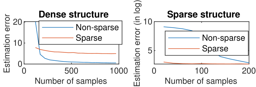
Figure 3: Estimation errors on (left) dense & (right) sparse struct.

5 Conclusions

In this paper, we proposed a method for learning sparse inverse covariance representation with CNN. Our method estimates SICE within the CNN layers and facilitates backpropagation for end-to-end training. Our iSICE significantly outperforms other covariance representations on several datasets. iSICE exploits the sparsity prior to capture partial correlations under limited number of samples. Our method is of general purpose and can be readily applied in existing SPD-based models to improve their performance.

Acknowledgements. This work was supported by CSIRO’s Machine Learning & Artificial Intelligence Future Science Platform (MLAI FSP), University of Wollongong’s Australia IPTA scholarship, and Australian Research Council (DP200101289). We thank Jianjia Zhang for discussions.

Learning Partial Correlation based Deep Visual Representation for Image Classification (Supplementary Material)

Saimunur Rahman^1,2, Piotr Koniusz^∗,1,3, Lei Wang², Luping Zhou⁴, Peyman Moghadam^1,5, Changming Sun^1
1Data61$\varheartsuit$CSIRO, ²University of Wollongong, ³Australian National University,
⁴University of Sydney ⁵Queensland University of Technology
name.surname@data61.csiro.au, leiw@uow.edu.au, luping.zhou@sydney.edu.au

Appendix A Datasets and the Evaluation Protocols

In this section, we provide the details of datasets and their evaluation protocols (see Section 4.1 of the main text). We perform experiments on eight widely used public image datasets, namely, MIT Indoor quattoni2009recognizing_supp, Stanford Cars krause20133d_supp, Caltech-UCSD Birds (CUB 200-2011) wah2011caltech_supp, FGVC-Aircraft maji2013fine_supp, DTD [5], iNaturalist [40], mini-ImageNet [41] and ImageNet100 imagenet100_supp to demonstrate the performance of our methods. Figure 4 shows the sample images from the datasets. Further details are given below.

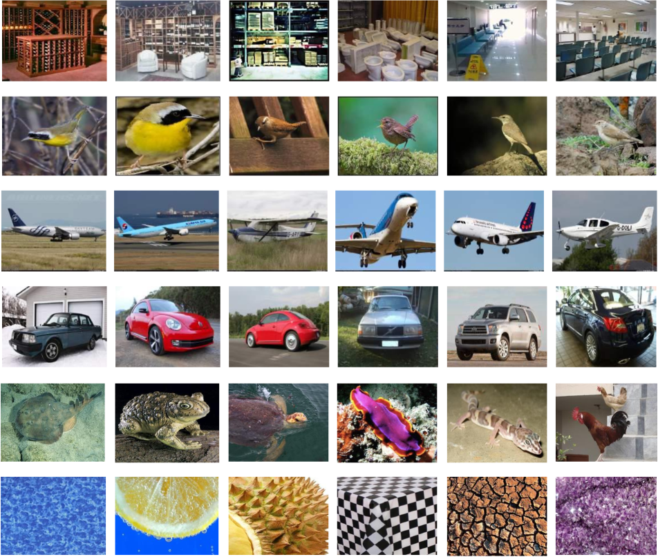
Figure 4: Sample images from the datasets used in our experiments. Rows 1, 2, 3, 4, 5 and 6 have the images from MIT Indoor, Caltech-UCSD Birds, FGVC-Aircraft, Stanford Cars, ImageNet100/mini-ImageNet and DTD datasets, respectively.

MIT Indoor dataset is one of the most widely used datasets in the literature for scene classification. It has a total of 15,620 images and 67 classes. Each image class contains a minimum number of 100 images. The images are collected from various types of stores (e.g., grocery, bakery), private places (e.g., bedroom and living room), public places (e.g., prison cell, bus, library), recreational places (e.g., restaurant, bar) and working environments (e.g., office, studio).

Caltech-UCSD Birds or simply ‘Birds’ is one of the most reported datasets in fine-grained image classification (FGIC) literature. It has a total of 11,788 images and 200 image classes. There are subtle differences between these classes and they are hard to be distinguished by human observers. This dataset comes with bounding box annotations; however, we do not use any annotations in our experiments.

FGVC-Aircraft or ‘Aircraft’ dataset is widely used by many recent FGIC methods. It has only 10,000 images distributed among 100 aircraft classes, and each class has precisely 100 images. Similar to Birds, the classes have subtle differences between them and are hard for humans to distinguish from each other.

Stanford Cars or simply ‘Cars’ has a total of 16,185 images and 196 classes. The classes are organized as per the car production year, car manufacturer and car model. Cars dataset has relatively smaller objects, i.e., cars, than those of the airplane dataset. Furthermore, the objects are appeared in cluttered backgrounds.

Describable Texture Dataset (DTD) has a total of 5,640 images and 47 classes. The images in all classes represents about 95% of their class attributes. For evaluation, it has 10 splits and each split has an equal number of images from each class for training, validation and test sets. The average performance across all splits is reported. We used both training and validation sets for training.

iNaturalist is a large fine-grained dataset. It has a total of 675,170 images and 5,089 classes. The classes are from 12 super-classes. The dataset is challenging due to its high class-imbalance. We use the training strategy and train-test splits specified in the original paper [40].

mini-ImageNet is a subset of ImageNet-1K dataset first proposed by Ravi et al. ravi2017optimization. It contains a total of 60,000 images and 100 classes. We use the original 224$\times$224 image resolution on this dataset. Since the dataset was originally proposed by the authors for few-shot learning tasks, we divide the dataset in a 90:10 ratio for training and testing. We report the average accuracy of 5 runs.

ImageNet100 is a subset of ImageNet-1K Dataset from ImageNet Large Scale Visual Recognition Challenge 2012. It contains random 100 classes proposed by Tian et al. imagenet100_supp. ImageNet100 train and validation sets contain 1300 and 50 images per class, respectively. We use the original 224$\times$224 image resolution on this dataset.

Dataset	Total classes	Total images	Predefined protocol		Major difficulty
			Training images	Testing images
MIT Indoor	67	6,700	5,360	1,340	difficult environment
Birds	200	11,788	5,994	5,794	subtle class difference
Aircraft	100	10,000	6,600	3,400	subtle class difference
Cars	196	16,185	8,144	8,041	cluttered background
DTD	47	5,640	4512	1128	complex structure
iNaturalist	5,089	675,170	579,184	95,986	class imbalance
mini-ImageNet	100	60,000	54,000	6,000	difficult environment
ImageNet100	100	1,35,000	130,000	5,000	difficult environment

Table 6: Summary of datasets.

Table 6 gives a more concise summary of the datasets. We train our method using the respective training splits provided by the original authors of the datasets. For evaluation, we again use the respective original test splits. This also applies to all of the methods we have compared in the main text. During training, for all datasets except iNaturalist, we resize our images to $448\times 448$ following the work of lin2015bilinear_supp,li2018towards_supp and use only horizontal flipping as a data augmentation. For iNaturalist, as in original paper, we resize images to $299\times 299$.

				iSICE
Dataset	Backbone	iSQRT-COV [23]	Precision $\mathbf{\Omega}$	Sparsity constant $\lambda$							Mean $\pm$ Std. (iSICE)
				1.0	0.5	0.1	0.01	0.001	0.0001	0.00001
MIT	VGG-16	76.12	80.15	77.46	78.13	78.13	78.66	78.58	78.96	78.96	78.41$\pm$0.54
	ResNet-50	78.81	80.75	78.43	80.75	80.45	80.52	80.90	80.37	81.34	80.39$\pm$0.93
Airplane	VGG-16	90.01	89.44	92.26	92.71	92.77	92.23	92.83	92.74	92.44	92.56 $\pm$0.25
	ResNet-50	90.88	91.15	92.89	92.65	92.89	92.74	92.83	92.56	92.56	92.73$\pm$0.14
Birds	VGG-16	84.47	83.36	86.04	86.47	86.35	86.52	85.59	86.31	86.28	86.22$\pm$0.32
	ResNet-50	84.26	84.67	84.62	85.16	85.30	85.90	86.05	85.90	85.59	85.50$\pm$0.51
Cars	VGG-16	91.21	92.04	93.60	93.98	94.06	94.03	93.88	93.91	93.50	93.85$\pm$0.22
	ResNet-50	92.13	91.99	93.01	93.36	93.69	93.51	93.22	93.72	93.40	93.41$\pm$0.25

Table 7: Performance of iSICE on changing the sparsity constant $\lambda$ while fixing the learning rate $\eta$ and the number of iterations ${N}$ to 1.0 and 5, respectively. The mean and standard deviation (std.) of the classification performance resulted by iSICE are also shown for a better understanding of sparsity constant changes in iSICE. Results are shown on multiple datasets with VGG-16 and ResNet-50 backbones. The best results in each row are highlighted with boldface.

				iSICE
Dataset	Backbone	iSQRT-COV [23]	Precision $\mathbf{\Omega}$	Learning rate $\eta$							Mean $\pm$ Std. (iSICE)
				0.001	0.01	0.1	1.0	5.0	10.0	20.0
MIT	VGG-16	76.12	80.15	78.81	79.33	77.91	78.66	78.28	80.52	77.76	78.75$\pm$0.95
	ResNet-50	78.81	80.75	80.82	80.82	80.75	80.52	81.19	79.33	78.96	80.34$\pm$0.85
Airplane	VGG-16	90.01	89.44	92.32	92.38	92.98	92.23	93.28	92.50	92.26	92.56$\pm$0.41
	ResNet-50	90.88	91.15	92.77	93.01	92.89	92.74	92.65	92.95	92.38	92.77$\pm$0.21
Birds	VGG-16	84.47	83.36	86.54	86.31	86.40	86.52	86.73	86.59	86.45	86.51$\pm$0.14
	ResNet-50	84.26	84.67	85.69	85.88	85.81	85.90	85.59	85.71	85.97	85.79$\pm$0.14
Cars	VGG-16	91.21	92.04	93.83	93.65	93.69	94.03	93.66	93.82	93.93	93.80$\pm$0.14
	ResNet-50	92.13	91.99	93.60	93.57	93.32	93.51	93.57	93.35	93.60	93.50$\pm$0.12

Table 8: Performance of iSICE on changing the learning rate $\eta$ while fixing the sparsity constant $\lambda$ and the number of iterations ${N}$ to 0.01 and 5, respectively. The mean and standard deviation (std.) of the classification performance resulted by iSICE are also shown for a better understanding of learning rate changes in iSICE. Results are shown on multiple datasets with VGG-16 and ResNet-50 backbones. The best results in each row are highlighted with boldface.

Method	Iter. ${N}$	Based on VGG-16 backbone				Based on ResNet-50 backbone
		MIT	Airplane	Birds	Cars	MIT	Airplane	Birds	Cars
iSQRT-COV [23]	5	76.12	90.01	84.47	91.21	78.81	90.88	84.26	92.13
Precision $\mathbf{\Omega}$	7	80.15	89.44	83.36	92.04	80.75	91.15	84.67	91.99
iSICE	2	78.28	92.68	86.66	93.63	80.52	92.89	93.68	85.92
	5	78.66	92.23	86.52	94.03	80.52	92.74	93.51	85.90
	10	78.36	92.56	86.62	93.89	80.22	92.74	93.30	85.74
Mean$\pm$Std. (iSICE)		78.4$\pm$0.2	92.5$\pm$0.2	86.6$\pm$0.1	93.9$\pm$0.2	80.4$\pm$0.2	92.8$\pm$0.1	93.5 $\pm$0.2	85.6 $\pm$ 0.1

Table 9: Performance of iSICE on changing number of iterations ${N}$ while fixing sparsity constant $\lambda$ and learning rate $\eta$ to 0.01 and 1.0, respectively. The mean and standard deviation (std.) of the classification performance resulted by iSICE are also shown (only single precision is shown for ease of presentation) for a better understanding of number of iterations changes in iSICE. Results are shown on multiple datasets with VGG-16 and ResNet-50 backbones. The best results in each column (including those that surpass the performance of iSQRT-COV) are highlighted with boldface.

Appendix B Training iSICE with Different Backbones

This section provides the settings of training different backbones with iSICE mentioned in Section 4.1 of the main text. We train iSICE with following backbones: VGG-16 simonyan2014very_supp, ResNet-50 he2016deep_supp, ConvNext-T liu2022convnet_supp, and Swin-T liu2021swin_supp. All backbones are pre-trained on ImageNet-1k deng2009imagenet_supp. We use the pre-trained weights provided by the torchvision 0.13.0 package that comes with PyTorch library paszke2019pytorch_supp.

All backbones produce more than 256 feature channels. In the recent literature on covariance representation li2017second_supp,li2018towards_supp,yu2018statistically_supp, a common practice is to experiment with 256 channels for efficiency and compactness of final representation. To compare our method with the recent literature, we also conducted most of our experiments with 256 channels. Additionally, we conducted experiments with 512 channels to demonstrate the effectiveness of the proposed iSICE in working with a larger number of feature channels (provided in Table 3 in the main text). For reducing the original number of feature channels from 2048/512 to 256, we add a $1\times 1$ convolution layer, batch normalisation and ReLU activation layers after the last convolution layer (in case of CNN models) and transformer block (in case of Swin Transformer). We then compute iSICE with the reduced feature channels, and we only use the upper-triangular entries of the symmetric matrix as a representation.

We fine-tune all backbones for 50-100 epochs with AdamW optimiser loshchilov2017decoupled_supp. We fine-tune VGG-16 and ResNet-50 CNN backbones with an initial learning rate of 0.00012, and ConvNext-T CNN and Swin-T transformer backbones with an initial learning rate 0.00005. For all backbones, we decrease the learning rate by a factor of 10 at the 15th and 30th epochs. Depending on the dataset and backbones, our fine-tuning process lasts for about 3-8 hours with four P100 GPUs, 12 CPUs and 12GB memory. We provide the source code of our method as supplement material for reproducing the experiments.

Appendix C Robustness of iSICE to Hyper-parameters

This section includes the experiments mentioned in “Robustness of iSICE on Hyper-parameter Changes” of Section 4.2 of the main text. We have conducted comprehensive experiments with the hyper-parameter range mentioned in the main text to demonstrate the robustness of iSICE with respect to hyper-parameter changes. In Tables 1, 2 and 3 of the main text, we showed the results obtained by using a consistent hyper-parameter set across different backbones and datasets to avoid overfitting. Specifically, we showed the results obtained with the median (marked with boldface) of the hyper-parameter range, i.e., $\lambda$ = {1.0, 0.5, 0.1, 0.01, 0.001, 0.0001, 0.00001}, $\eta$ = {0.001, 0.01, 0.1, 1.0, 5.0, 10.0, 20.0}, and ${N}$ = {1, 5, 10}.

Below we show some experiments to demonstrate the robustness of iSICE with respect to hyper-parameter changes. Specifically, we analyse the performance of iSICE when one hyper-parameter changes while the other two are fixed. For consistency, we experiment with the same hyper-parameters used for reporting the performance of iSICE across the tables of the main text, i.e., $\lambda$ = 0.01, $\eta$ = 1.0, and ${N}$ = 5. As mentioned above, we will fix two of them and vary the third one to observe its impact to the performance of the proposed iSICE. All of our experiments are compared with COV and Precision $\mathbf{\Omega}$ methods (please refer to the main text for details).

Robustness against sparsity constant changes. In this experiment, we change the sparsity constant $\lambda$ while keeping the learning rate $\eta$ and the number of iterations ${N}$ fixed. Our experimental results are shown in Table 7. From the results, we can clearly see that across all datasets, the change of sparsity constants does not significantly impact the performance of iSICE. The VGG-16 based iSICE shows more robustness toward sparsity constant changes. The classification performance for the MIT dataset appears to have been more significantly impacted due to sparsity constant changes than the other three fine-grained datasets. Specifically, on the three fine-grained datasets, the standard deviation of results is significantly low, i.e., less than 0.51 when compared with the mean values ranging between 85.50 to 93.85. This confirms that our method can be used for fine-grained image classification purposes with a reasonable range of sparsity constant.

Changing the learning rate. In this experiment, we change the learning rate while keeping the sparsity constant and the number of iterations fixed. Our experimental results are shown in Table 8. From the results, we can see that across all datasets, the change in learning rate does not significantly affect the performance. Two datasets, namely Birds and Cars, have shown less impact on performance, as suggested by the standard deviation of 0.14 or lower. The other two datasets also show a low standard deviation of results. The low standard deviation across a wide range of learning rates (from 0.001 to 20.0) shows that our method is robust to the changes in learning rate and a small learning rate such as 0.01 can be used for computing SICE with our method.

Changing the number of iterations. Below we change the number of iterations while keeping the sparsity constant and the learning rate fixed. Our experimental results are shown in Table 9. The results show that regardless of the CNN backbones used, the change in the number of iterations can vary the performance only up to 0.20. It is also noticeable that our method is able to give good performance even with two iterations only. This experiment shows that our method is not sensitive to the changes in the number of iterations.

Appendix D iSICE with Learning Rate and Sparsity Modulators

This section provides additional experiments on iSICE with MLP modulators introduced in “iSICE with learning rate and sparsity modulators” of Section 4.2 of the main text. In Table 4, the CNN feature maps with average pooling were used to learn on-the-fly the learning rate and sparsity. In Table 10, we provide an additional experiment with MLP when both $\nabla_{1}$ from Alg. 2 and average-pooled feature maps are used, i.e., concatenated before passing them into the modulator. The combination of $\nabla_{1}$ from Alg. 2 and average-pooled feature maps further improve the classification performance of iSICE.

Method	MIT	Airplane	Birds	Cars	ImageNet100
iSICE	80.5	92.7	85.9	93.5	74.8
iSICE+MLP	81.3	93.4	86.1	93.9	76.3
iSICE+MLP∗	81.8	93.8	86.4	93.9	77.1

Table 10: Comparison between the classification performance of iSICE, iSICE+MLP and iSICE+MLP^∗ (improved variant) on ResNet-50. Results of iSICE+MLP in second row use X to compute learning rate and sparsity with modulators. Results of iSICE+MLP^∗ in the third row use a concatenation of both X and $\Delta_{1}$ from Alg. 2 to compute on-the-fly learning rate and sparsity by MLP-based modulators.

Appendix E Memory Consumption

This section describes memory consumption on iSICE mentioned. Algorithm 2 stores the $d\times{d}$ matrices of ${\mathbf{\Sigma}}$, ${\mathbf{S}}_{i}$, ${\mathbf{S}}^{+}_{i}$ and ${\mathbf{S}}^{-}_{i}$, etc. The memory complexity of Algorithm 2 is approximately $\mathcal{O}\big{(}d^{2}(N\!+\!N_{s})\big{)}$, where $d$ denotes the channel size, $N$ is iSICE iterations, and $N_{s}$ is Newton-Schulz iterations. For typical $d=256$, $N=5$, $N_{s}=5$, iSICE uses approximately $3\times 10\times 8\times 256^{2}=0.012$ GB memory which is a tiny fraction of memory that the backbone consumes.

Appendix F Visualisation of Learned Feature Maps

Below we visualize the convolutional feature maps learned by the CNN model with different methods. We extract feature maps from the last convolution layer and perform average pooling on them. We convert the pooled feature map to a heatmap and draw it over the input image. The colour in the heatmap ranges from blue to red, blue indicates cold and red indicates hot. Fig. 5 suggests that with iSICE, the model focuses well on the key parts of car to extract features for classification. GAP (global average pooling) overly focuses on entire foreground, iSQRT focuses poorly, while iSICE lets us control the degree of ‘focus’ by controlling sparsity.

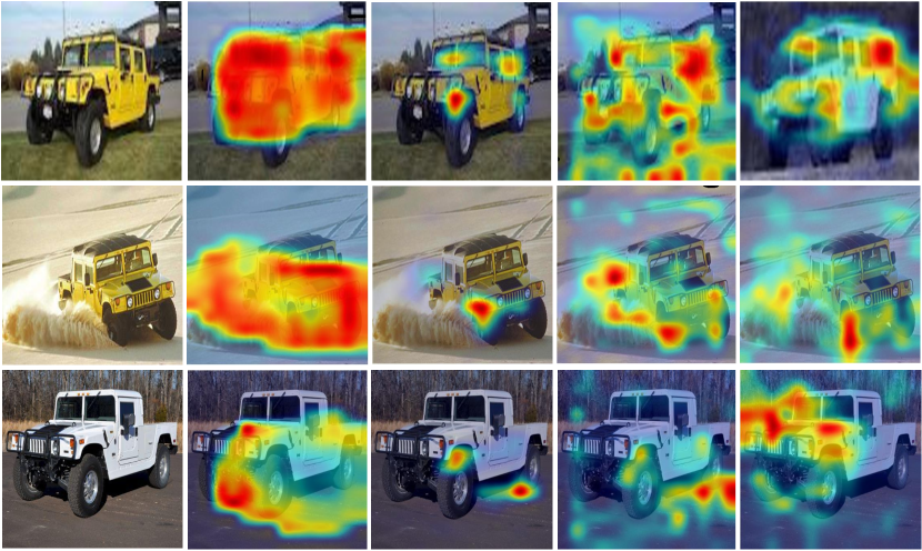
Figure 5: Visualisation of learned convolutional feature maps from Cars dataset with ResNeXt-101 backbone. From left: Input image, GAP, iSQRT-COV, Precision Matrix and iSICE.

ieee_fullname latex

References

- [1] Akshay Agrawal, Brandon Amos, Shane Barratt, Stephen Boyd, Steven Diamond, and J Zico Kolter. Differentiable convex optimization layers. Advances in neural information processing systems, 32, 2019.
- [2] Relja Arandjelovic, Petr Gronat, Akihiko Torii, Tomas Pajdla, and Josef Sivic. Netvlad: Cnn architecture for weakly supervised place recognition. In Proceedings of the IEEE conference on computer vision and pattern recognition, pages 5297–5307, 2016.
- [3] Stephen Boyd, Neal Parikh, Eric Chu, Borja Peleato, Jonathan Eckstein, et al. Distributed optimization and statistical learning via the alternating direction method of multipliers. Foundations and Trends® in Machine learning, 3(1):1–122, 2011.
- [4] Sijia Cai, Wangmeng Zuo, and Lei Zhang. Higher-order integration of hierarchical convolutional activations for fine-grained visual categorization. In Proceedings of the IEEE international conference on computer vision, pages 511–520, 2017.
- [5] Mircea Cimpoi, Subhransu Maji, Iasonas Kokkinos, Sammy Mohamed, and Andrea Vedaldi. Describing textures in the wild. In Proceedings of the IEEE conference on computer vision and pattern recognition, pages 3606–3613, 2014.
- [6] Yin Cui, Feng Zhou, Jiang Wang, Xiao Liu, Yuanqing Lin, and Serge Belongie. Kernel pooling for convolutional neural networks. In Proceedings of the IEEE conference on computer vision and pattern recognition, pages 2921–2930, 2017.
- [7] Morris H. DeGroot. Optimal statistical decisions. McGraw-Hill, New York, NY [u.a], 1970.
- [8] Steven Diamond and Stephen Boyd. Cvxpy: A python-embedded modeling language for convex optimization. The Journal of Machine Learning Research, 17(1):2909–2913, 2016.
- [9] Melih Engin, Lei Wang, Luping Zhou, and Xinwang Liu. Deepkspd: Learning kernel-matrix-based spd representation for fine-grained image recognition. In Proceedings of the European Conference on Computer Vision, pages 612–627, 2018.
- [10] Jerome Friedman, Trevor Hastie, and Robert Tibshirani. Sparse inverse covariance estimation with the graphical lasso. Biostatistics, 9(3):432–441, 2008.
- [11] Yang Gao, Oscar Beijbom, Ning Zhang, and Trevor Darrell. Compact bilinear pooling. In Proceedings of the IEEE conference on computer vision and pattern recognition, pages 317–326, 2016.
- [12] Trevor Hastie, Robert Tibshirani, Jerome H Friedman, and Jerome H Friedman. The elements of statistical learning: data mining, inference, and prediction, volume 2. Springer, 2009.
- [13] Kaiming He, Xiangyu Zhang, Shaoqing Ren, and Jian Sun. Deep residual learning for image recognition. In Proceedings of the IEEE conference on computer vision and pattern recognition, pages 770–778, 2016.
- [14] Nicholas J Higham. Functions of matrices: theory and computation. SIAM, 2008.
- [15] Junzhou Huang, Tong Zhang, and Dimitris Metaxas. Learning with structured sparsity. Journal of Machine Learning Research, 12(11), 2011.
- [16] Catalin Ionescu, Orestis Vantzos, and Cristian Sminchisescu. Matrix backpropagation for deep networks with structured layers. In Proceedings of the IEEE international conference on computer vision, pages 2965–2973, 2015.
- [17] Shu Kong and Charless Fowlkes. Low-rank bilinear pooling for fine-grained classification. In Proceedings of the IEEE conference on computer vision and pattern recognition, pages 365–374, 2017.
- [18] Piotr Koniusz, Lei Wang, and Anoop Cherian. Tensor representations for action recognition. IEEE Transactions on Pattern Analysis and Machine Intelligence, 44(2):648–665, 2021.
- [19] Piotr Koniusz, Fei Yan, Philippe-Henri Gosselin, and Krystian Mikolajczyk. Higher-order occurrence pooling on mid-and low-level features: Visual concept detection. Tech. Report (hal-00922524), 2013.
- [20] Piotr Koniusz and Hongguang Zhang. Power normalizations in fine-grained image, few-shot image and graph classification. In IEEE Transactions on Pattern Analysis and Machine Intelligence. IEEE, 2021.
- [21] Jonathan Krause, Michael Stark, Jia Deng, and Li Fei-Fei. 3d object representations for fine-grained categorization. In Proceedings of the IEEE international conference on computer vision workshops, pages 554–561, 2013.
- [22] Miroslav Kubat. Neural networks: a comprehensive foundation by simon haykin, macmillan, 1994, isbn 0-02-352781-7. The Knowledge Engineering Review, 13(4):409–412, 1999.
- [23] Peihua Li, Jiangtao Xie, Qilong Wang, and Zilin Gao. Towards faster training of global covariance pooling networks by iterative matrix square root normalization. In Proceedings of the IEEE conference on computer vision and pattern recognition, pages 947–955, 2018.
- [24] Peihua Li, Jiangtao Xie, Qilong Wang, and Wangmeng Zuo. Is second-order information helpful for large-scale visual recognition? In Proceedings of the IEEE international conference on computer vision, pages 2070–2078, 2017.
- [25] Tsung-Yu Lin and Subhransu Maji. Improved bilinear pooling with cnns. British Machine Vision Conference, 2017.
- [26] Tsung-Yu Lin, Subhransu Maji, and Piotr Koniusz. Second-order democratic aggregation. In Proceedings of the European Conference on Computer Vision, pages 620–636, 2018.
- [27] Tsung-Yu Lin, Aruni RoyChowdhury, and Subhransu Maji. Bilinear cnn models for fine-grained visual recognition. In Proceedings of the IEEE international conference on computer vision, pages 1449–1457, 2015.
- [28] Tsung-Yu Lin, Aruni RoyChowdhury, and Subhransu Maji. Bilinear convolutional neural networks for fine-grained visual recognition. IEEE transactions on pattern analysis and machine intelligence, 40(6):1309–1322, 2017.
- [29] Ze Liu, Yutong Lin, Yue Cao, Han Hu, Yixuan Wei, Zheng Zhang, Stephen Lin, and Baining Guo. Swin transformer: Hierarchical vision transformer using shifted windows. In Proceedings of the IEEE/CVF International Conference on Computer Vision, pages 10012–10022, 2021.
- [30] Zhuang Liu, Hanzi Mao, Chao-Yuan Wu, Christoph Feichtenhofer, Trevor Darrell, and Saining Xie. A convnet for the 2020s. In Proceedings of the IEEE/CVF Conference on Computer Vision and Pattern Recognition, pages 11976–11986, 2022.
- [31] Ilya Loshchilov and Frank Hutter. Decoupled weight decay regularization. arXiv preprint arXiv:1711.05101, 2017.
- [32] Subhransu Maji, Esa Rahtu, Juho Kannala, Matthew Blaschko, and Andrea Vedaldi. Fine-grained visual classification of aircraft. arXiv preprint arXiv:1306.5151, 2013.
- [33] Ariadna Quattoni and Antonio Torralba. Recognizing indoor scenes. In 2009 IEEE conference on computer vision and pattern recognition, pages 413–420. IEEE, 2009.
- [34] Saimunur Rahman, Lei Wang, Changming Sun, and Luping Zhou. Redro: Efficiently learning large-sized spd visual representation. In European Conference on Computer Vision, pages 1–17. Springer, 2020.
- [35] Bernt Schiele, Paul Swoboda, and Gerard Pons-Moll. Projected gradient descent for the lasso. Lecture Notes, 2018.
- [36] Christian Simon, Piotr Koniusz, Richard Nock, and Mehrtash Harandi. On modulating the gradient for meta-learning. In Proceedings of the European conference on computer vision, 2020.
- [37] Karen Simonyan and Andrew Zisserman. Very deep convolutional networks for large-scale image recognition. arXiv preprint arXiv:1409.1556, 2014.
- [38] Yue Song, Nicu Sebe, and Wei Wang. Why approximate matrix square root outperforms accurate svd in global covariance pooling? In Proceedings of the IEEE/CVF International Conference on Computer Vision, pages 1115–1123, 2021.
- [39] Yonglong Tian, Dilip Krishnan, and Phillip Isola. Contrastive multiview coding. In European conference on computer vision, pages 776–794. Springer, 2020.
- [40] Grant Van Horn, Oisin Mac Aodha, Yang Song, Yin Cui, Chen Sun, Alex Shepard, Hartwig Adam, Pietro Perona, and Serge Belongie. The inaturalist species classification and detection dataset. In Proceedings of the IEEE conference on computer vision and pattern recognition, pages 8769–8778, 2018.
- [41] Oriol Vinyals, Charles Blundell, Timothy Lillicrap, Daan Wierstra, et al. Matching networks for one shot learning. Advances in neural information processing systems, 29, 2016.
- [42] Catherine Wah, Steve Branson, Peter Welinder, Pietro Perona, and Serge Belongie. The caltech-ucsd birds-200-2011 dataset. 2011.
- [43] Qilong Wang, Jiangtao Xie, Wangmeng Zuo, Lei Zhang, and Peihua Li. Deep cnns meet global covariance pooling: Better representation and generalization. IEEE transactions on pattern analysis and machine intelligence, 43(8):2582–2597, 2020.
- [44] Ruiping Wang, Huimin Guo, Larry S Davis, and Qionghai Dai. Covariance discriminative learning: A natural and efficient approach to image set classification. In 2012 IEEE conference on computer vision and pattern recognition, pages 2496–2503. IEEE, 2012.
- [45] Saining Xie, Ross Girshick, Piotr Dollár, Zhuowen Tu, and Kaiming He. Aggregated residual transformations for deep neural networks. In Proceedings of the IEEE conference on computer vision and pattern recognition, pages 1492–1500, 2017.
- [46] Kaicheng Yu and Mathieu Salzmann. Statistically-motivated second-order pooling. In Proceedings of the European Conference on Computer Vision, pages 600–616, 2018.
- [47] Tan Yu, Yunfeng Cai, and Ping Li. Toward faster and simpler matrix normalization via rank-1 update. In European Conference on Computer Vision, pages 203–219. Springer, 2020.
- [48] Tan Yu, Xiaoyun Li, and Ping Li. Fast and compact bilinear pooling by shifted random maclaurin. In Proceedings of the AAAI Conference on Artificial Intelligence, volume 35, pages 3243–3251, 2021.
- [49] Tan Yu, Xiaoyun Li, and Ping Li. Efficient compact bilinear pooling via kronecker product. In Proceedings of the AAAI Conference on Artificial Intelligence, volume 36, pages 3170–3178, 2022.
- [50] Hongguang Zhang, Jing Zhang, and Piotr Koniusz. Few-shot learning via saliency-guided hallucination of samples. In Proceedings of the IEEE/CVF Conference on Computer Vision and Pattern Recognition, pages 2770–2779, 2019.
- [51] Jianjia Zhang, Lei Wang, Luping Zhou, and Wanqing Li. Beyond covariance: Sice and kernel based visual feature representation. International Journal of Computer Vision, 129(2):300–320, 2021.
- [52] Shan Zhang, Dawei Luo, Lei Wang, and Piotr Koniusz. Few-shot object detection by second-order pooling. In Proceedings of the Asian conference on computer vision, 2020.
- [53] Shan Zhang, Naila Murray, Lei Wang, and Piotr Koniusz. Time-reversed diffusion tensor transformer: A new tenet of few-shot object detection. In Proceedings of the European conference on computer vision, 2022.
- [54] Shan Zhang, Lei Wang, Naila Murray, and Piotr Koniusz. Kernelized few-shot object detection with efficient integral aggregation. In Proceedings of the IEEE/CVF Conference on Computer Vision and Pattern Recognition, 2022.
- [55] Yifei Zhang, Hao Zhu, Zixing Song, Piotr Koniusz, and Irwin King. Spectral feature augmentation for graph contrastive learning and beyond. In Proceedings of the AAAI Conference on Artificial Intelligence, 2023.