From Hyperbolic to Parabolic Parameters
along Internal Rays

Abstract

For the quadratic family $f_{c}(z)=z^{2}+c$ with $c$ in a hyperbolic component of the Mandelbrot set, it is known that every point in the Julia set moves holomorphically. In this paper we give a uniform derivative estimate of such a motion when the parameter $c$ converges to a parabolic parameter ${\hat{c}}$ radially; in other words, it stays within a bounded Poincaré distance from the internal ray that lands on ${\hat{c}}$. We also show that the motion of each point in the Julia set is uniformly one-sided Hölder continuous at ${\hat{c}}$ with exponent depending only on the petal number.

This paper is a parabolic counterpart of the authors’ paper “From Cantor to semi-hyperbolic parameters along external rays” (Trans. Amer. Math. Soc. 372 (2019) pp. 7959–7992).

1 Introduction and main results

Hyperbolic components.

Let $\mathbb{M}$ be the Mandelbrot set, the connectedness locus of the quadratic family

$${\left\{f_{c}:z\mapsto z^{2}+c\right\}}_{c\,\in\,\mathbb{C}}.$$

That is, the Julia set $J(f_{c})$ is connected if and only if $c\in\mathbb{M}$. A parameter $c\in\mathbb{M}$ is called hyperbolic if $f_{c}$ has a (super-)attracting periodic point. Equivalently, there exist positive numbers $\gamma_{c}$ and $\varepsilon_{c}$ such that $|Df_{c}^{n}(z)|\geq\gamma_{c}(1+\varepsilon_{c})^{n}$ for any $n\geq 0$ and $z\in J(f_{c})$. The set of hyperbolic parameters in $\mathbb{M}$ is an open subset and its connected components are called hyperbolic components of the Mandelbrot set. (The complement of $\mathbb{M}$ is also called a hyperbolic component, but in this paper we only consider those contained in the Mandelbrot set.)

Let $\mathbb{D}$ be the unit disk in $\mathbb{C}$ and $\mathbb{X}$ a hyperbolic component of $\mathbb{M}$. Sullivan and Douady-Hubbard (see [DH, Exposés XIV & XIX] and [Mi, Thm.6.5]) gave a uniformization of $\mathbb{X}$, which is a canonical homeomorphism $\Phi=\Phi_{\mathbb{X}}:\overline{\mathbb{D}}\to\overline{\mathbb{X}}$ such that $\Phi|_{\mathbb{D}}:\mathbb{D}\to\mathbb{X}$ is an conformal isomorphism; and for any $c=\Phi(\mu)$ with $\mu\in\overline{\mathbb{D}}-\{1\}$, the map $f_{c}$ has a periodic point of multiplier $\mu$ with a common period. The parameters $\Phi(0)$ and $\Phi(1)$ in $\overline{\mathbb{X}}$ are called the center and the root of $\mathbb{X}$ respectively. Note that the Poincaré distance in $\mathbb{X}$ is defined by pulling-back the Poincaré (hyperbolic) metric $|dz|/(1-|z|^{2})$ on $\mathbb{D}$ by the isomorphism $\Phi$.

Internal rays and thick internal rays.

For a given hyperbolic component $\mathbb{X}$ and a given real number $\theta$, we define the internal ray $I(\theta)$ of angle $\theta$ by

$$I(\theta)=I_{\mathbb{X}}(\theta):={\left\{\Phi(re^{2\pi i\theta})\in\mathbb{X}\,:\,0\leq r<1\right\}}.$$

The point

$${\hat{c}}:=\Phi(e^{2\pi i\theta})\in\partial\mathbb{X}$$

is called the landing point of $I(\theta)$. For a given $\delta\geq 0$, we define the $\delta$-thick internal ray ${\mathcal{I}}(\theta,\delta)$ of angle $\theta$ by the closed $\delta$-neighborhood of $I(\theta)$ in $\mathbb{X}$ with respect to the Poincaré distance. We say the parameter $c$ tends to ${\hat{c}}$ along a thick internal ray if there exists a $\delta\geq 0$ such that $c$ stays in the $\delta$-thick internal ray ${\mathcal{I}}(\theta,\delta)$ while it tends to ${\hat{c}}$. It is rather common to say that such a $c$ converges to ${\hat{c}}$ radially (after McMullen [Mc2]) or non-tangentially. Indeed, for any angle $A_{0}\in[0,\pi/2)$, if $c$ stays in the $\delta(A_{0})$-thick internal ray with

$$\delta(A_{0})=\frac{1}{2}\log\frac{1+\tan(A_{0}/2)}{1-\tan(A_{0}/2)}\in[0,\infty),$$ (1.1)

then by letting $\mu_{c}:=\Phi^{-1}(c)$ and $\hat{\mu}:=\Phi^{-1}({\hat{c}})$ we have

$${\left|\arg{\left(1-\frac{\mu_{c}}{\hat{\mu}}\right)}\right|}\leq A_{0}$$

for $c$ sufficiently close to ${\hat{c}}$. In other words, $\mu_{c}$ stays in the Stolz angle at $\hat{\mu}\in\partial\mathbb{D}$ with opening angle $2A_{0}$. (See [P, p.7] and Figure 4 in the next section.)

Holomorphic motion of the hyperbolic Julia sets.

It is well-known that there exists a holomorphic motion ([BR, L, Mc1, MSS]) of the Julia sets over any hyperbolic component $\mathbb{X}$ of $\mathbb{M}$. Indeed, we have an equivariant holomorphic motion as follows. For any base point $\sigma\in\mathbb{X}$, there exists a unique map $H:\mathbb{X}\times J(f_{\sigma})\to\mathbb{C}$ such that

1. $H(\sigma,z)=z$ for any $z\in J(f_{\sigma})$.

2. For any $c\in\mathbb{X}$, the map $z\mapsto{H}(c,z)$ is injective on $J(f_{\sigma})$.

3. For any $z\in J(f_{\sigma})$, the map $c\mapsto H(c,{z})$ is holomorphic on $\mathbb{X}$.

4. For any $c\in\mathbb{X}$, the map $h_{c}(z):=H(c,z)$ satisfies $h_{c}(J(f_{\sigma}))=J(f_{c})$ and $f_{c}\circ h_{c}=h_{c}\circ f_{\sigma}$ on $J(f_{\sigma})$.

See [Mc1, §4] for more details. In this paper we choose the center $\sigma:=\Phi(0)$ of $\mathbb{X}$ as the base point of the motion. We are concerned with boundary behavior of such an equivariant holomorphic motion of the Julia set $J(f_{\sigma})$ when $c\in\mathbb{X}$ tends to some ${\hat{c}}\in\partial\mathbb{X}$ along a thick internal ray.

Parabolic parameters.

Now suppose that the angle $\theta$ of the internal ray $I(\theta)$ is a rational number. Then for the landing point ${\hat{c}}$ of $I(\theta)$, $f_{\hat{c}}$ has a parabolic periodic point, that is, a periodic point whose multiplier is a root of unity. We say such a parameter ${\hat{c}}$ is parabolic, and a parabolic periodic point ${\hat{b}}$ of $f_{\hat{c}}$ has $q$ petals if the local dynamics of $f_{\hat{c}}^{k}$ near ${\hat{b}}$ is of the form $\zeta\mapsto\zeta+\zeta^{q+1}+O(\zeta^{q+2})$ for some $k$ in an appropriate local coordinate. In our setting, it is known that ${\hat{b}}$ has $q$ petals if and only if the multiplier of ${\hat{b}}$ is a primitive $q$-th root of unity (since $f_{\hat{c}}$ is quadratic and has only one critical point in $\mathbb{C}$).

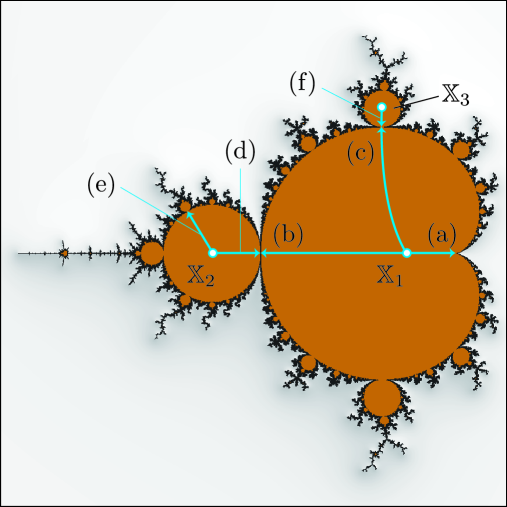
Figure 1: Internal rays (a) – (f) of the Mandelbrot set.

Example 1 (Period one, the main cardioid).

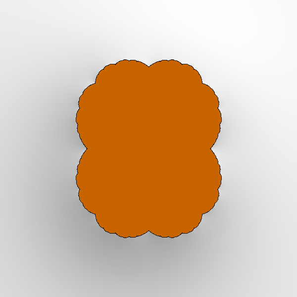
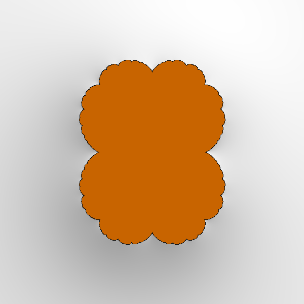
(a): $I(0)$ in $\mathbb{X}_{1}$

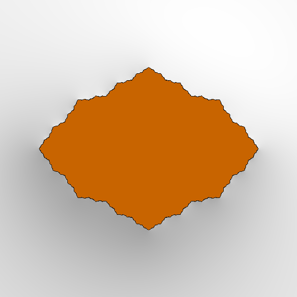
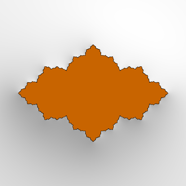
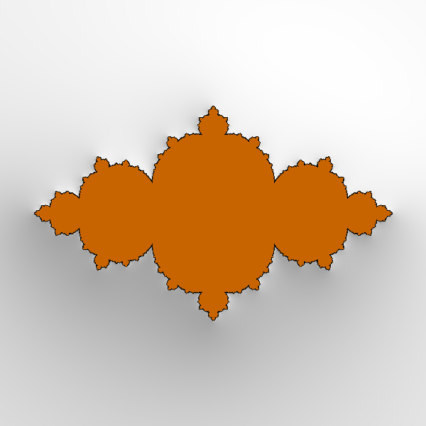
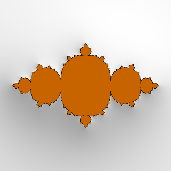
(b): $I(1/2)$ in $\mathbb{X}_{1}$

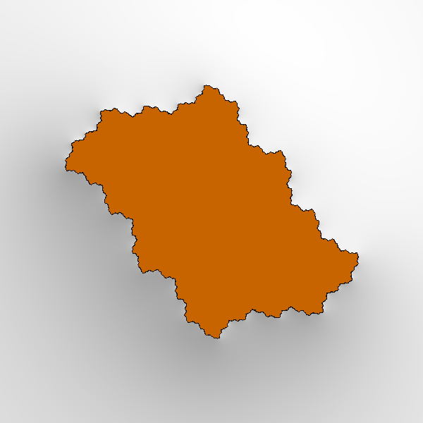
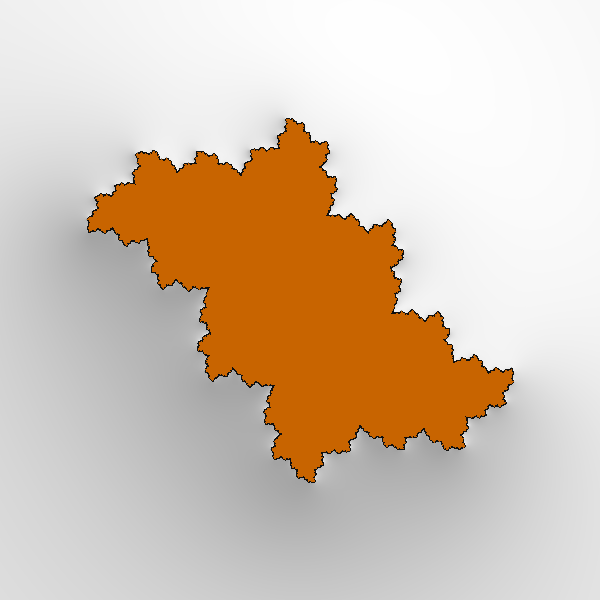
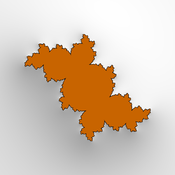
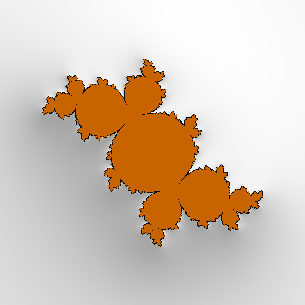
(c): $I(1/3)$ in $\mathbb{X}_{1}$

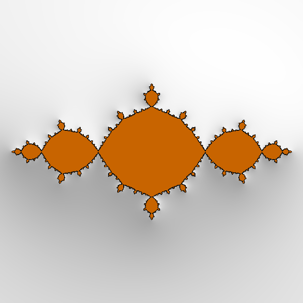
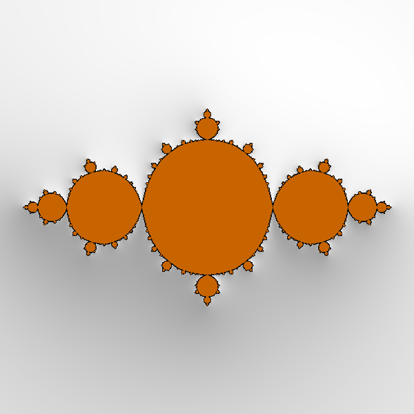
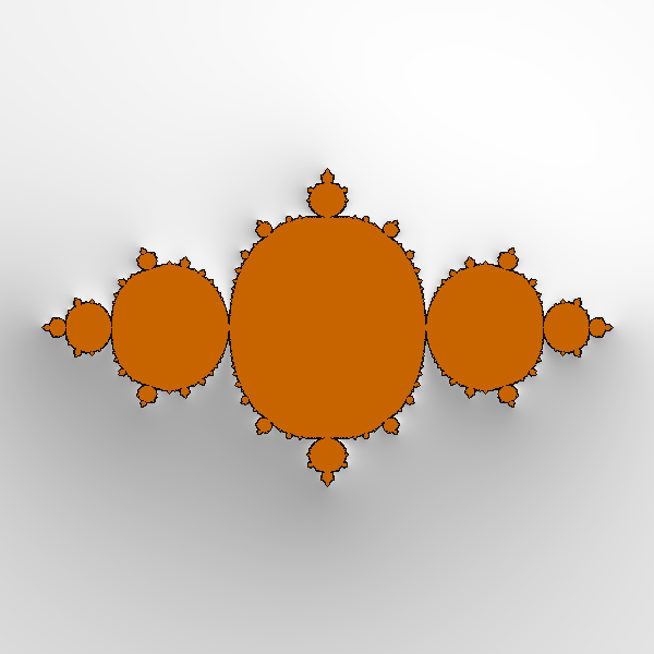
(d): $I(0)$ in $\mathbb{X}_{2}$

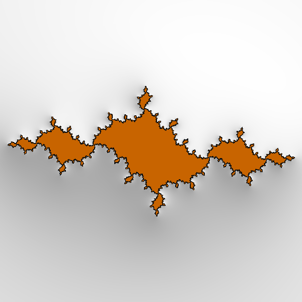
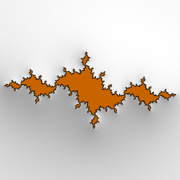
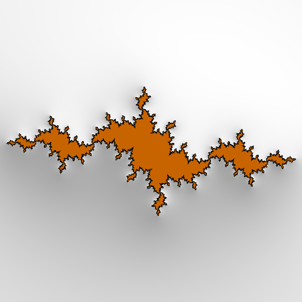
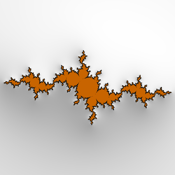
(e): $I(1/3)$ in $\mathbb{X}_{2}$

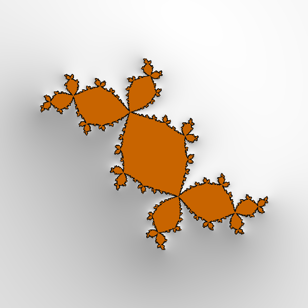
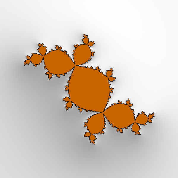
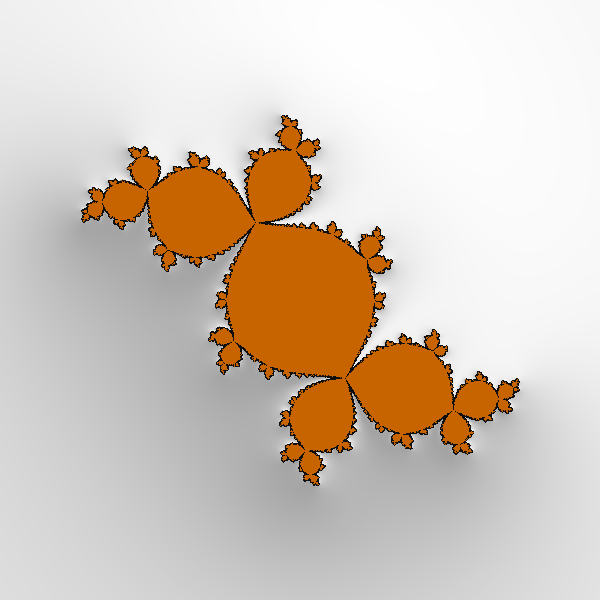
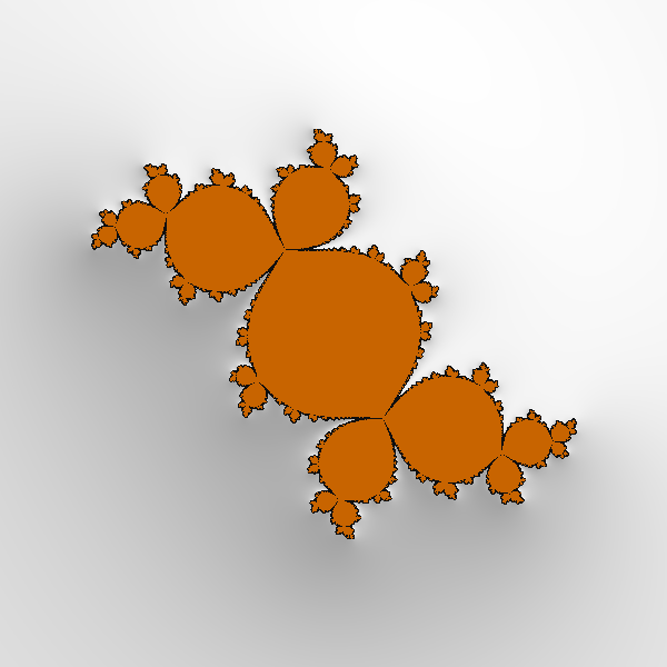
(f): $I(0)$ in $\mathbb{X}_{3}$

Figure 3: Holomorphic motions along the internal rays depicted in Figure 1.

For the hyperbolic component $\mathbb{X}_{1}$ containing $0$ (the main cardioid), the map $\Phi=\Phi_{\mathbb{X}_{1}}$ is explicitly given by $\Phi(\mu):=-\mu^{2}/4+\mu/2~{}(\mu\in\overline{\mathbb{D}})$ and $f_{\Phi(\mu)}$ has a fixed point with multiplier $\mu$. The internal ray of angle $\theta$ is given by $I_{\mathbb{X}_{1}}(\theta)={\left\{-r^{2}e^{4\pi\theta i}/4+re^{2\pi\theta i}/2\,:\,0\leq r<1\right\}}.$ In Figure 1, $I_{\mathbb{X}_{1}}(\theta)$ for $\theta=0,1/2$ and $1/3$ are depicted as paths (a), (b), and (c) respectively. The corresponding holomorphic motions along $I_{\mathbb{X}_{1}}(0)$ and $I_{\mathbb{X}_{1}}(1/2)$ are illustrated in Figure 2 and in Figures 3(a) and 3(b). The motion along $I_{\mathbb{X}_{1}}(1/3)$ is depicted in Figure 3(c).

Example 2 (Period two).

Similarly the hyperbolic component $\mathbb{X}_{2}$ containing $-1$ consists of hyperbolic parameters $c$ such that $f_{c}$ has an attracting cycle of period two. The map $\Phi=\Phi_{\mathbb{X}_{2}}$ is explicitly given by $\Phi(\mu):=\mu/4-1$ for $\mu\in\overline{\mathbb{D}}$, and $f_{\Phi(\mu)}$ with $\mu\in\overline{\mathbb{D}}-\{1\}$ has a periodic point of period two with multiplier $\mu$. The internal ray of angle $\theta$ is given by $I_{\mathbb{X}_{2}}(\theta)={\left\{re^{2\pi\theta i}/4-1\,:\,0\leq r<1\right\}}.$ In Figure 1, $I_{\mathbb{X}_{2}}(\theta)$ for $\theta=0$ and $1/3$ are depicted as paths (d) and (e) respectively. The internal ray $I_{\mathbb{X}_{2}}(0)$ lands at the root ${\hat{c}}=\Phi(1)=-3/4$ of $\mathbb{X}_{2}$, where the map $f_{\hat{c}}$ has a parabolic fixed point of multiplier $-1$ that has two petals. Note that ${\hat{c}}$ is the landing point of another internal ray $I_{\mathbb{X}_{1}}(1/2)$ of $\mathbb{X}_{1}$. See Figures 3(d) and 3(e) for the motions along $I_{\mathbb{X}_{2}}(0)$ and $I_{\mathbb{X}_{2}}(1/3)$.

Example 3 (Period three).

There is a hyperbolic component $\mathbb{X}_{3}$ attached to the main cardioid $\mathbb{X}_{1}$ that consists of parameters $c$ with $\mathrm{Im}\,c>0$ for which $f_{c}$ has an attracting cycle of period three. The internal ray $I_{\mathbb{X}_{3}}(0)$ (depicted as path (f) in Figure 1) joins the center (so-called “rabbit”) and the root ${\hat{c}}=\Phi(1)$ (“the fat rabbit”), where the map $f_{\hat{c}}$ has a parabolic fixed point of multiplier $e^{2\pi i/3}$ that has three petals. (See Figure 3(f) for the holomorphic motion along $I_{\mathbb{X}_{3}}(0)$.) Again ${\hat{c}}$ is the landing point of another internal ray $I_{\mathbb{X}_{1}}(1/3)$ of $\mathbb{X}_{1}$.

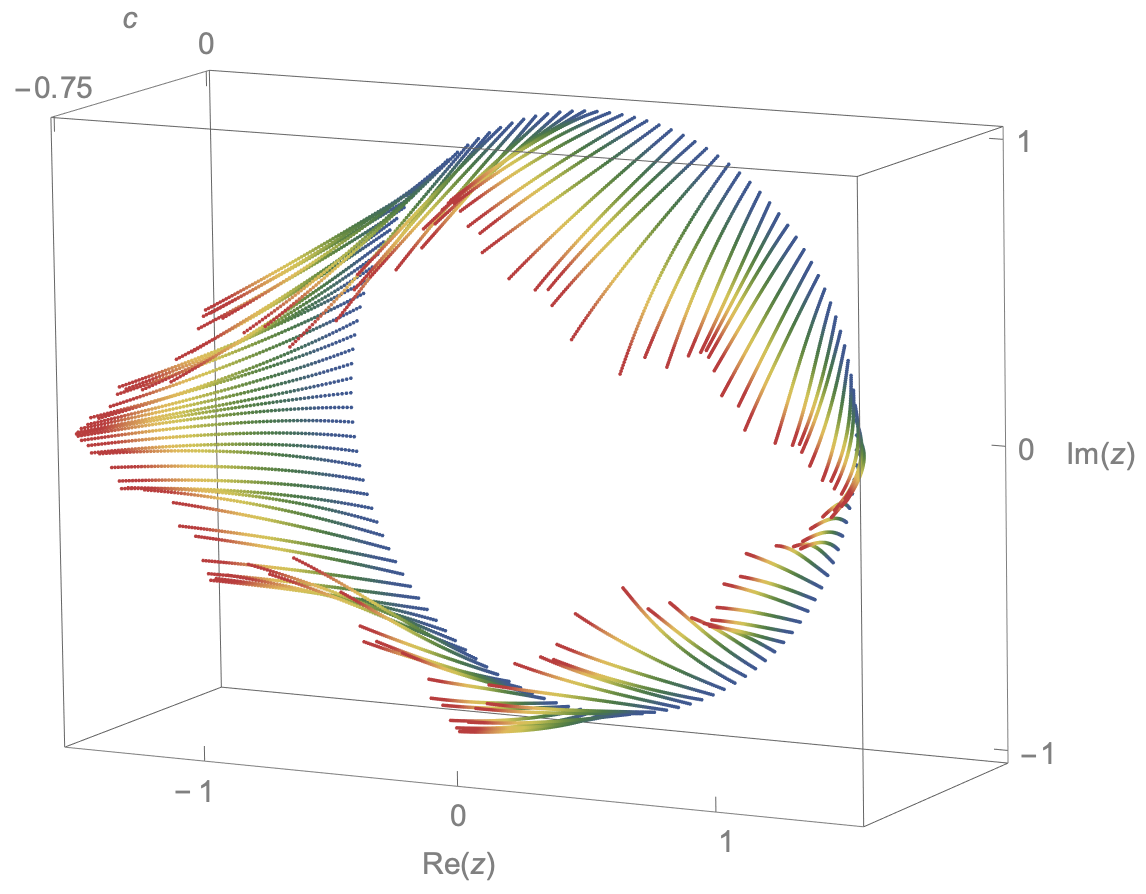
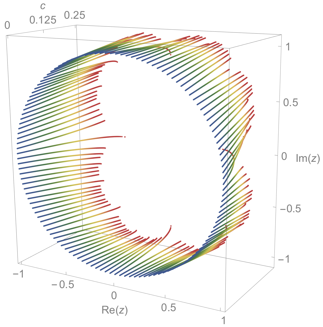
Figure 2: Real analytic motion of the preimages of the repelling fixed point along the internal rays $I(1/2)$ (left) and $I(0)$ (right) in $\mathbb{X}_{1}$.

Main results.

Let $\mathbb{X}$ be a hyperbolic component in the Mandelbrot set and $\sigma$ be its center. For any $z_{\ast}$ in $J(f_{\sigma})$, the map $c\mapsto z(c):=H(c,z_{\ast})$ is holomorphic over $\mathbb{X}$. Let ${\hat{c}}\in\partial\mathbb{X}$ be the landing point of the internal ray $I_{\mathbb{X}}(\theta)$ of rational angle $\theta$. Our main theorem states that the speed of $z(c)=H(c,z_{\ast})$ is uniformly bounded by a function of $|c-{\hat{c}}|$ as $c$ tends to ${\hat{c}}$ along a thick internal ray:

Theorem 1.1 (Main Theorem).

Suppose that $f_{\hat{c}}$ has a parabolic periodic point with $q$ petals and $c$ tends to ${\hat{c}}$ along a thick internal ray ${\mathcal{I}}(\theta,\delta)$ in $\mathbb{X}$. Then there exists a constant $K>0$ depending only on ${\hat{c}}$ and $\delta$ such that for any $z=z(c)\in J(f_{c})$, the point $z(c)$ moves holomorphically with

$${\left|\frac{d}{dc}z(c)\right|}\leq\frac{K}{{\left|\,c-{\hat{c}}\,\right|}^{1-1/Q}},$$

where $Q=\max\{2,q\}$.

By this theorem we obtain one-sided Hölder continuity of the holomorphic motion along thick internal rays landing on parabolic parameters:

Theorem 1.2 (One-sided Hölder Continuity).

Under the same assumption as Theorem 1.1 above, the point $z=z(c)$ in $J(f_{c})$ tends to a limit $z({\hat{c}})$ in $J(f_{\hat{c}})$ as $c$ tends to ${\hat{c}}$ along the thick internal ray ${\mathcal{I}}(\theta,\delta)$. Moreover, there exists a constant $K^{\prime}$ depending only on ${\hat{c}}$ and $\delta$ such that

$$|z(c)-z({\hat{c}})|\leq K^{\prime}|\,c-{\hat{c}}\,|^{1/Q}$$ (1.2)

for any $c$ in ${\mathcal{I}}(\theta,\delta)$.

As an immediate consequence the holomorphic motion of each point $z(c)\in J(f_{c})$ lands when $c$ moves along the internal ray $I(\theta)={\mathcal{I}}(\theta,0)$. This theorem yields a precise description of the degeneration of the dynamics on the Julia sets along the internal rays of rational angles:

Theorem 1.3 (Pinching Semiconjugacy).

Under the same assumption as the theorems above, the conjugacy $H(c,\cdot)=h_{c}:J(f_{\sigma})\to J(f_{c})$ converges uniformly to a semiconjugacy $h_{{\hat{c}}}:J(f_{\sigma})\to J(f_{\hat{c}})$ from $f_{\sigma}$ to $f_{{\hat{c}}}$ as $c$ tends to ${\hat{c}}$ along the thick internal ray $I(\theta,\delta)$. Moreover, $h_{\hat{c}}$ satisfies the following:

1. If ${\hat{c}}$ is the root of $\mathbb{X}$, then $h_{{\hat{c}}}$ is injective and thus a conjugacy.

2. If ${\hat{c}}$ is not the root of $\mathbb{X}$ (hence $q\geq 2)$, then the preimage $h_{\hat{c}}^{-1}(\{w\})$ of any $w\in J(f_{\hat{c}})$ consists of one or $q$ distinct points, and the latter holds if and only if $w$ eventually lands on a parabolic periodic point of $f_{\hat{c}}$.

3. The semiconjugacy $\eta_{c}:=h_{\hat{c}}\circ h_{c}^{-1}:J(f_{c})\to J(f_{\hat{c}})$ satisfies

   $$|\eta_{c}(z)-z|\leq K^{\prime}|c-{\hat{c}}|^{1/Q}$$ (1.3)

   for any $c$ in the thick internal ray ${\mathcal{I}}(\theta,\delta)$.

By (3) of this theorem we obtain:

Corollary 1.4 (Hausdorff Convergence).

The Hausdorff distance between $J(f_{c})$ and $J(f_{\hat{c}})$ is $O(|c-{\hat{c}}|^{1/Q})$ as $c$ tends to ${\hat{c}}$ along a thick internal ray.

Remark 1.5.

• These results are parabolic counterparts of the authors’ results in [CK1] about parameter rays (external rays) landing on semi-hyperbolic parameters of the Mandelbrot set.

• For any $c\in\mathbb{X}$ and $z=z(c)\in J(f_{c})$, we have

  $${\left|\frac{d}{dc}{z}(c)\right|}\leq\frac{\,1+\sqrt{1+6\,|c|\,}\,}{\mathrm{dist}\,(c,\partial\mathbb{X})}$$ (1.4)

  by Proposition 3.1 in [CK1]. However, this will only give

  $${\left|\frac{d}{dc}{z}(c)\right|}=O{\left(\frac{1}{|c-{\hat{c}}|}\right)}$$

  as $c$ tends to ${\hat{c}}$.

• In [CK2], the authors showed that for any $c\in[0,1/4)=I_{\mathbb{X}_{1}}(0)$ and $z=z(c)\in J(f_{c})$, we have an optimal estimate

  $${\left|\frac{d}{dc}{z}(c)\right|}\leq\frac{1}{2\sqrt{1/4-c}}.$$

  In particular, the Hausdorff distance between $J(f_{c})$ and $J(f_{1/4})$ is exactly $\sqrt{1/4-c}$.

• The existence of the semiconjugacy in Theorem 1.3 and the Hausdorff convergence of the Julia sets in Corollary 1.4 are previously shown in a more general context by the second author [K1] and McMullen [Mc2] respectively. The novel part of our results is the quantitative estimate $O(|c-{\hat{c}}|^{1/Q})$.

Structure of the paper.

In Section 2, we define a parametrization of $c$ with a complex parameter $t\in\mathbb{C}$ such that $c=c_{t}$ converges to ${\hat{c}}$ along a thick internal ray as $t\to 0$. Also in Section 2, we state three propositions, Propositions 2.2, 2.3 and 2.4, which concern the local dynamics of $f_{c}$ in a neighborhood $U_{0}$ of a parabolic point of $f_{\hat{c}}$ when $c$ is near ${\hat{c}}$, and will be employed to prove Theorems 1.2 and 1.3 as well as some lemmas in the paper. Then, we introduce the notion of “S-cycle” to describe how an orbit of $f_{c}$ repeatedly (infinite or finite times or never) enters and leaves a fixed subset of $U_{0}$. In Section 3, by assuming Lemmas A, B and C, we prove our main theorem, Theorem 1.1. It is well-known (for example [Mc1, §3.2]) that the Julia set is expanding with respect to the hyperbolic metric on $\mathbb{C}-P(f_{c})$, where $P(f_{c})$ denotes the postcritical set of $f_{c}$. In order to estimate the expansion of the Julia set with respect to the Euclidean metric, we give an estimate of the distance between $z\in J(f_{c})$ and $P(f_{\hat{c}})$ in Lemma D in Section 4 for $z$ not too close to the parabolic cycle of $f_{\hat{c}}$. Lemma A is proved in Section 5 by assuming another two lemmas, Lemmas G and H. Both lemmas rely on local dynamics of perturbed parabolic cycle. We prove Lemma B in Section 6, and Lemma G in Section 8. Section 7 is devoted to the proofs of Propositions 2.2 and 2.3. We use a branched coordinate to prove Proposition 2.4 in Section 9. We also employ the branched coordinate to prove Lemma H in Section 10. Then, using some results presented in Section 10, we are able to prove Lemma D in Section 11. Some arguments in the proofs of Lemmas H and D are used to prove Lemma C in Section 12. Finally, in Section 13 we prove Theorems 1.2 and 1.3 simultaneously.

2 Radial access condition and S-cycles

In this section we introduce the notion of S-cycles for a given orbit in the Julia set. The idea of S-cycles was introduced in [CK1] to describe orbits that repeatedly come close to the postcritical set. Here we present a modified version where the postcritical set is replaced by the parabolic cycle.

Notation.

We start with some notation and the terminology that will be used in what follows.

• Let $\mathbb{N}$ denote the set of positive integers. We denote the set of non-negative integers by $\mathbb{N}_{0}:=\{0\}\cup\mathbb{N}$.

• Let $\mathbb{D}(a,r)$ denote the disk in $\mathbb{C}$ centered at $a$ and of radius $r>0$. When $a=0$ we denote it by $\mathbb{D}(r)$.

• For non-negative variables $X$ and $Y$, by $X\asymp Y$ we mean there exists an implicit constant $C>1$ independent of $X$ and $Y$ such that $X/C\leq Y\leq CX$.

• When we say “for any $X\ll 1$” it means that “for any sufficiently small $X>0$”. More precisely, we mean there exists an implicit constant $C>0$ such that $0<X<C$.

Hyperbolic components and internal rays.

Let ${\hat{c}}\in\partial\mathbb{M}$ be a parabolic parameter having a parabolic periodic point ${\hat{b}}$ of period exactly $p$. Let $\hat{\lambda}:=Df_{{\hat{c}}}^{p}({\hat{b}})$ be the multiplier of this cycle, and assume that it is a primitive $q$-th root of unity. We specify an internal ray $I(\theta)=I_{\mathbb{X}}(\theta)$ of the hyperbolic component $\mathbb{X}$ that lands at ${\hat{c}}$ as follows. (See [DH] or [Mi] for details on the hyperbolic components of $\mathbb{M}$.)

Case 1.

If $q=1$, then there is only one hyperbolic component $\mathbb{X}$ such that ${\hat{c}}=\Phi_{\mathbb{X}}(1)\in\partial\mathbb{X}$, where $\Phi_{\mathbb{X}}$ is the uniformizing map of $\mathbb{X}$. Hence by letting $\theta=0$ the internal ray $I(\theta)$ of $\mathbb{X}$ lands at ${\hat{c}}$.

Case 2.

If $q\geq 2$, then there are exactly two hyperbolic components $\mathbb{X}^{-}$ and $\mathbb{X}^{+}$ such that

• $\partial\mathbb{X}^{-}\cap\partial\mathbb{X}^{+}=\{{\hat{c}}\}$.

• ${\hat{c}}=\Phi_{\mathbb{X}^{-}}(\hat{\lambda})$ and ${\hat{c}}=\Phi_{\mathbb{X}^{+}}(1)$, where $\Phi_{\mathbb{X}^{\pm}}$ is the uniformizing map of $\mathbb{X}^{\pm}$.

Hence $\mathbb{X}$ can be either $\mathbb{X}^{-}$ or $\mathbb{X}^{+}$, and the case of $q\geq 2$ is divided into two sub-cases.

• Case 2^-: If $\mathbb{X}=\mathbb{X}^{-}$, then we let $\theta=(\arg\hat{\lambda})/(2\pi)$; and

• Case 2⁺: If $\mathbb{X}=\mathbb{X}^{+}$, then we let $\theta=0$

in such a way that the internal ray $I(\theta)=I_{\mathbb{X}}(\theta)$ of $\mathbb{X}$ lands at ${\hat{c}}$.

Note that ${\hat{c}}$ is the root of $\mathbb{X}$ if and only if it is as Case 1 or Case 2⁺. Hence,

$$\theta=\left\{\begin{array}[]{ll}0&\text{for {Case 1} or {Case 2${}^{+}$},}\\[3.01385pt] (\arg\hat{\lambda})/(2\pi)&\text{for {Case 2${}^{-}$}.}\end{array}\right.$$

Example 4.

Case 1 holds when ${\hat{c}}=1/4$ with $\mathbb{X}=\mathbb{X}_{1}$ (Example 1), or ${\hat{c}}=-7/4$ with $\mathbb{X}$ whose center is a unique real parameter $\sigma<0$ with $f_{\sigma}^{3}(0)=0$ (“the airplane”). If $\hat{c}=-3/4$, Case 2^- holds when $\mathbb{X}^{-}=\mathbb{X}_{1}$, and Case 2⁺ holds when $\mathbb{X}^{+}=\mathbb{X}_{2}$ (Example 2).

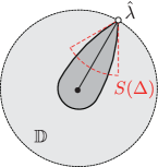
Figure 4: The Stolz angle $S(\Delta)$ with opening angle $2A_{0}$ equal to $\pi/3$ at $\hat{\lambda}\in\partial\mathbb{D}$. The dark gray region is the image of $\delta$-thick internal ray ${\mathcal{I}}(\theta,\delta)$ under $\Phi^{-1}$ with $\delta=\delta(A_{0})$.

Radial convergence and thick internal rays.

Let $A_{0}$ and $T_{0}$ be constants with $0\leq A_{0}<\pi/2$ and $0<T_{0}<2\cos A_{0}$, and let

$$\Delta=\Delta(A_{0},T_{0}):=\{t\in\mathbb{C}\,:\,0<|t|\leq T_{0},~{}|\arg t\,|\leq A_{0}\}.$$

The Stolz angle at $\hat{\lambda}$ with opening angle $2A_{0}$ is given by

$$S(\Delta):=\{\mu=(1-t)\hat{\lambda}\in\mathbb{D}\,:\,t\in\Delta\}\subset\mathbb{D}.$$ (2.1)

Let $\Phi:=\Phi_{\mathbb{X}}$. If the parameter $c\in\mathbb{X}$ tends to ${\hat{c}}$ satisfying $\Phi(c)\in S(\Delta)$, we say $c\to{\hat{c}}$ radially after McMullen [Mc2].

For a given $\delta$-thick internal ray ${\mathcal{I}}(\theta,\delta)\subset\mathbb{X}$ of angle $\theta$, one can easily check that

$$\Phi^{-1}({\mathcal{I}}(\theta,\delta))\cap\mathbb{D}(\hat{\lambda},T_{0})\subset S(\Delta)$$

if $\delta\leq\delta(A_{0})$, which is given in (1.1). See Figure 4. Hence in what follows it is enough to consider the parameters of the form $c=\Phi(\mu)$ with $\mu\in S(\Delta)\cup\{\hat{\lambda}\}$.

Remark 2.1.

Conversely, the Stolz angle $S(\Delta)$ is contained in $\Phi^{-1}({\mathcal{I}}(\theta,\delta))$ with $\delta=\delta(A_{0})+1$ by taking a sufficiently small $T_{0}$. This implies that the convergence in a thick internal ray is equivalent to the radial convergence for some angle.

Parametrization and notation.

For a technical reason, instead of (2.1), it is convenient to re-parametrize $\mu\in S(\Delta)$ by

$$\mu=\mu_{t}:=\left\{\begin{array}[]{ll}1-q\,t&\text{in {Case 1} or {Case 2${}^{+}$}}\\[3.01385pt] (1-t/q)\hat{\lambda}&\text{in {Case 2${}^{-}$}}\end{array}\right.$$

for $t\in\Delta=\Delta(A_{0},T_{0})$ with sufficiently small $T_{0}$.

The radial access condition.

In what follows, by

$$c\approx{\hat{c}}\quad\text{or}\quad c=c_{t}\approx{\hat{c}}$$

we mean the parameter $c$ is of the form

$$c=c_{t}=\Phi(\mu_{t})$$

for some $t\in\Delta=\Delta(A_{0},T_{0})$, where we take a smaller $T_{0}$ in the definition of $\Delta$ if necessary. We say such a parameter $c$ satisfies the radial access condition or $c$ is in a thick internal ray.

Perturbation of parabolic points.

Let $c_{0}:={\hat{c}}$ and $\lambda_{0}:=\hat{\lambda}$. In Section 7, we will show the following two propositions under the radial access condition:

Proposition 2.2.

The function $t\mapsto c=c_{t}$ is holomorphic on $\Delta$, and there exists a constant $B_{0}\neq 0$ such that

• Case 1 ($q=1$): $c_{t}={\hat{c}}+B_{0}t^{2}+O(t^{3})$

• Case 2^± ($q\geq 2$): $c_{t}={\hat{c}}+B_{0}t+O(t^{2})$

as $t\in\Delta$ tends to $0$. In particular, we have $\sqrt{|c_{t}-{\hat{c}}|}\asymp|t|$ or $|c_{t}-{\hat{c}}|\asymp|t|$ for $t\in\Delta$ according to Case 1 or Case 2^±.

Proposition 2.3.

There exists a continuous map $t\mapsto b_{t}$ defined for $t\in\Delta\cup\{0\}$ such that

1. $b_{0}=\hat{b}$ and $b_{t}$ is a periodic point of $f_{c_{t}}$ with the same period $p$ as ${\hat{b}}$.

2. Let $\lambda_{t}:=Df_{c_{t}}^{p}(b_{t})$. Then there exist two families of holomorphic local coordinates ${\left\{\zeta=\varphi_{t}(z)\right\}}_{t\,\in\,\Delta\cup\{0\}}$ and ${\left\{w=\psi_{t}(z)\right\}}_{t\,\in\,\Delta\cup\{0\}}$ defined on a disk $\hat{U}:=\mathbb{D}({\hat{b}},\hat{R})$ such that: For each $z\in\hat{U}$, $\varphi_{t}(z)$ and $\psi_{t}(z)$ are holomorphic in $t\in\Delta$ and continuous at $t=0$; $\varphi_{t}(b_{t})=\psi_{t}(b_{t})=0$; and

   $$\varphi_{t}\circ f_{c_{t}}^{p}\circ\varphi_{t}^{-1}(\zeta) =\lambda_{t}\zeta+\zeta^{q+1}+O(\zeta^{2q+1}),~{}\text{and}$$ (2.2)

   $$\psi_{t}\circ f_{c_{t}}^{pq}\circ\psi_{t}^{-1}(w) =\lambda_{t}^{q}w\,(1+w^{q}+O(w^{2q})).$$ (2.3)

   In particular, both $D\varphi_{t}^{-1}(0)$ and $D\psi_{t}^{-1}(0)$ are uniformly bounded away from zero.

3. In Case 1 or Case 2⁺, $b_{t}$ is repelling for $t\in\Delta$, and the multiplier satisfies

   $$\lambda_{t}=(1+t/q+o(t))\,\hat{\lambda}.$$

   Moreover, there are $q$ distinct attracting fixed points $\alpha_{t}^{1},\,\cdots,\,\alpha_{t}^{q}$ of $f_{c_{t}}^{pq}$ satisfying $Df_{c_{t}}^{pq}(\alpha_{t}^{j})=\mu_{t}=1-qt$ and $\left(\psi_{t}(\alpha_{t}^{j})\right)^{q}=-t+o(t)$ for $j=1,\cdots,q$.

4. In Case 2^-, $b_{t}$ is attracting for $t\in\Delta$ and the multiplier satisfies

   $$\lambda_{t}=\mu_{t}=(1-t/q)\,\hat{\lambda}.$$

   Moreover, there are $q$ distinct repelling fixed points $\beta_{t}^{1},\,\cdots,\,\beta_{t}^{q}$ of $f_{c_{t}}^{pq}$ satisfying $Df_{c_{t}}^{pq}(\beta_{t}^{j})=1+qt+o(t)$ and $\left(\psi_{t}(\beta_{t}^{j})\right)^{q}=t+o(t)$ for $j=1,\cdots,q$.

The local dynamics of $f_{c_{t}}^{pq}$ observed as (2.3) behaves quite similar to that of $f_{{\hat{c}}}^{pq}$. See Figure 5. In particular, in the domain $\hat{U}=\mathbb{D}({\hat{b}},\hat{R})$ of $\psi_{t}$, the map $f_{c_{t}}^{pq}$ has exactly

• one repelling fixed point $b_{t}$ in Case 1 or Case 2⁺; and

• $q$ repelling fixed points in Case 2^- that are symmetrically arrayed near $b_{t}$.

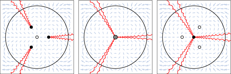
Figure 5: The middle frame depicts the local dynamics of $f_{{\hat{c}}}^{pq}$ near $\hat{U}$ (indicated by the big circle) that can be mildly perturbed in two ways: Case 2^- on the left, and Case 2⁺ on the right. The white, black, and gray dots indicate attracting, repelling, and parabolic fixed points respectively. The red spiky curves indicate the Julia sets.

Definition of $U_{0}$.

We fix a small $R_{0}\in(0,\hat{R})$ such that the disk

$$U_{0}:=\mathbb{D}({\hat{b}},R_{0})\quad(\Subset\hat{U})$$

possesses the property that $f_{\hat{c}}^{p}:U^{\prime}\to U_{0}$ is univalent for each connected component $U^{\prime}$ of $f_{\hat{c}}^{-p}(U_{0})$. Such an $R_{0}$ exists because the orbit $f_{\hat{c}}^{n}(0)$ of $0$ (the critical point) keeps a definite distance from the parabolic cycle for $0\leq n\leq p$. The next proposition will be proved in Section 9:

Proposition 2.4.

For each parameter $c_{t}$ with $t\in\Delta$ if $z_{0}\in J(f_{c_{t}})\cap U_{0}$ is none of the repelling fixed points of $f_{c_{t}}^{pq}$ described as above, then the orbit $z_{kpq}:=f_{c_{t}}^{kpq}(z_{0})~{}(k\in\mathbb{N}_{0})$ leaves $U_{0}$ for some $k>0$.

We choose some $\xi\in(0,1]$ such that

$$\mathrm{dist}\,(0,f_{\hat{c}}^{k}(U_{0}))\geq\frac{3\xi}{4}$$

for any integer $k$ with $-p\leq k\leq p$. Note that by continuity, we have

$$\mathrm{dist}\,(0,f_{c}^{k}(U_{0}))\geq\frac{\xi}{2}$$

for any $c\approx{\hat{c}}$ (taking a smaller $T_{0}$ in the definition of $\Delta$ if necessary) and any $k$ with $-p\leq k\leq p$.

Remark 2.5.

We will frequently use the following property: If $z\in f_{c}^{k}(U_{0})$ for some $c\approx{\hat{c}}$ and $k$ with $-p\leq k\leq p$, then $|Df_{c}(z)|=2|z|\geq\xi$.

Definition of $V_{0}$ and ${\mathcal{V}}(c)$.

Now we take a small $\nu\in(0,R_{0})$ and let

$$V_{0}:=\mathbb{D}({\hat{b}},\nu)\quad(\Subset U_{0}).$$

We also define

$${\mathcal{V}}(c):=\bigcup_{j=0}^{p-1}f_{c}^{-j}(V_{0})$$

for each $c\approx{\hat{c}}$. By Remark 2.5 above, $f_{c}(z)\in{\mathcal{V}}(c)$ implies $|Df_{c}(z)|\geq\xi$ for $c\approx{\hat{c}}$.

S-cycles.

For $c\approx{\hat{c}}$, let $z_{0}$ be any point in the Julia set $J(f_{c})$. The orbit $z_{n}:=f_{c}^{n}(z_{0})~{}(n\in\mathbb{N}_{0})$ may land on $V_{0}$ ($\Subset U_{0}$), and leave $U_{0}$ by Proposition 2.4 (unless it lands exactly on the repelling cycle), then it may come back to $V_{0}$ again. To describe the behavior of such an orbit, we introduce the notion of “S-cycle” for the orbit of $z_{0}$, where “S” indicates that orbit stays near the “singularity” of the hyperbolic metric $\rho(z)|dz|$ on the complement of the postcritical set of $f_{\hat{c}}$ to be defined in Section 4.

Definition (S-cycle).

A finite S-cycle of the orbit $z_{n}=f_{c}^{n}(z_{0})~{}(n\in\mathbb{N}_{0})$ is a finite subset of $\mathbb{N}_{0}$ of the form

$${\sf S}={\left\{n\in\mathbb{N}_{0}\,:\,M\leq n<M^{\prime}\right\}}=[M,M^{\prime})\cap\mathbb{N}_{0}$$

with the following properties:

• $z_{M}\in V_{0}$, and if $M>0$ then $z_{M-1}\notin V_{0}$.

• There exists a minimal $m\geq 1$ such that for $n=M+mpq$, $z_{n-pq}\in U_{0}$ but $z_{n}\notin U_{0}$.

• $M^{\prime}=M+mpq+L$ for some $L\in[1,\infty)$ such that $z_{n}\notin V_{0}$ for $n=M+mpq+i~{}(0\leq i<L)$ and $z_{M^{\prime}}\in V_{0}$.

An infinite S-cycle ${\sf S}$ of the orbit $z_{n}=f_{c}^{n}(z_{0})~{}(n\in\mathbb{N}_{0})$ is an infinite subset of $\mathbb{N}_{0}$ of the form

$${\sf S}={\left\{n\in\mathbb{N}_{0}\,:\,M\leq n<\infty\right\}}=[M,\infty)\cap\mathbb{N}_{0},$$

satisfying either

• Type (I): (S1), (S2), and

  • $z_{n}\notin V_{0}$ for all $n\geq M+mpq$;

or

• Type (II): (S1) and

  • $z_{M+kpq}\in V_{0}$ for any $k\in\mathbb{N}$. Equivalently, $z_{M}$ is a repelling periodic point of period $p$ or period $pq$ in $V_{0}$ (by Proposition 2.4).

By an S-cycle we mean a finite or infinite S-cycle. In both cases, we denote them by ${\sf S}=[M,M^{\prime})$ or ${\sf S}=[M,\infty)$ for brevity.

Remark 2.6.

We may assume without loss of generality that $L$ of the finite S-cycle is at least $p$ by shrinking the radius of the disk $U_{0}$. Indeed, after the orbit $z_{n}~{}(n\in\mathbb{N}_{0})$ leaves $U_{0}$ when $n=M+mpq$, the orbit follows the parabolic cycle for a while and it cannot land immediately on $V_{0}$ by the local dynamics near the perturbed cycle. See Figure 6.

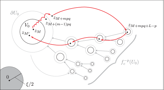
Figure 6: A finite S-cycle $[M,M^{\prime})$ with $M^{\prime}=M+mpq+L$, $p=3$. The dotted arrow indicates there is another connected component of $f_{c}^{-p}(U_{0})$ intersecting with $U_{0}$ which is not drawn.

Decomposition of the orbit by S-cycles.

For a given orbit $z_{n}=f_{c}^{n}(z_{0})~{}(n\in\mathbb{N}_{0})$ of $z_{0}\in J(f_{c})$, the set $\mathbb{N}_{0}$ of indices is uniquely decomposed by using finite or infinite S-cycles in one of the following three types:

• The first type is of the form

  $$\mathbb{N}_{0}=[0,M_{1})\sqcup{\sf S}_{1}\sqcup{\sf S}_{2}\sqcup\cdots,$$ (2.4)

  where $z_{n}\notin V_{0}$ for $n\in[0,M_{1})$ and ${\sf S}_{k}:=[M_{k},M_{k+1})$ is a finite S-cycle for each $k\geq 1$.

• The second type is of the form

  $$\mathbb{N}_{0}=[0,M_{1})\sqcup{\sf S}_{1}\sqcup{\sf S}_{2}\sqcup\cdots\sqcup{\sf S}_{k_{0}}\sqcup\emptyset\sqcup\emptyset\sqcup\cdots$$ (2.5)

  with $k_{0}\geq 1$, where $z_{n}\notin V_{0}$ for $n\in[0,M_{1})$; ${\sf S}_{k}:=[M_{k},M_{k+1})$ is a finite S-cycle for each $1\leq k\leq k_{0}-1$; ${\sf S}_{k_{0}}=[M_{k_{0}},\infty)$ is an infinite S-cycle; and ${\sf S}_{k}=\emptyset$ for $k\geq k_{0}+1$.

• The third type is

  $$\mathbb{N}_{0}=[0,M_{1})\sqcup\emptyset\sqcup\emptyset\sqcup\cdots$$ (2.6)

  with $M_{1}=\infty$ and ${\sf S}_{k}=\emptyset$ for $k\geq 1$, where $z_{n}\notin V_{0}$ for all $n\in\mathbb{N}$.

In the first and second types it is possible that $M_{1}=0$ and $[0,M_{1})$ is empty.

3 Proof of the main theorem assuming three lemmas

The derivative formula.

Let $z_{\ast}$ be any point in $J(f_{\sigma})$ (where $\sigma$ is the center of $\mathbb{X}$), and consider its motion $z=z(c)=H(c,z_{\ast})\in J(f_{c})$ for $c\in\mathbb{X}$. The estimate of the main theorem is based on the following formula:

Proposition 3.1 (The Derivative Formula).

For any $c\in\mathbb{X}$ and $z=z(c)\in J(f_{c})$, we have

$$\frac{d}{dc}{z}(c)=-\sum_{n=1}^{\infty}\frac{1}{Df_{c}^{{n}}({z}(c))}.$$

See [CK1, Proposition 3.2] for the proof. Since $f_{c}$ is hyperbolic, the convergence of the series above is absolute and it is enough to show

$$\left|\sum_{n=1}^{\infty}\frac{1}{Df_{c}^{{n}}({z}(c))}\right|\leq\frac{K}{|c-{\hat{c}}|^{1-1/Q}}$$

for some constant $K>0$ independent of $c$ in a thick internal ray, where $Q:=\max\{2,\,q\}$ and $q$ is the petal number of the parabolic fixed point ${\hat{b}}$.

Now we present three principal lemmas about S-cycles that are valid for sufficiently small $\nu$ (the radius of $V_{0}$) under the radial access condition $c=c_{t}\approx{\hat{c}}$. That is, we only consider $c=c_{t}$ with $t\in\Delta=\Delta(A_{0},T_{0})$ as in the previous section.

Lemma A.

There exists a constant $K_{\mathrm{A}}>0$ such that for any $c\approx{\hat{c}}$, any $z_{0}\in J(f_{c})$, and for any S-cycle ${\sf S}=[M,M^{\prime})$ of the orbit $z_{n}=f_{c}^{n}(z_{0})~{}(n\in\mathbb{N}_{0})$, we have

$$\left|\sum_{i=1}^{M^{\prime}-M}\frac{1}{Df_{c}^{i}(z_{M})}\right|\leq\frac{K_{\mathrm{A}}}{|c-{\hat{c}}|^{1-1/Q}},$$ (3.1)

where we set $M^{\prime}-M:=\infty$ if $M^{\prime}=\infty$.

Lemma B.

There exists a constant $K_{\mathrm{B}}>0$ such that for any $c\approx{\hat{c}}$ and any $M\leq\infty$, if $z_{0}\in J(f_{c})$ satisfies $z_{n}\notin V_{0}$ for any $n\in[0,M)$, then we have

$$\sum_{i=1}^{M}\frac{1}{|Df_{c}^{i}(z_{0})|}\leq K_{\mathrm{B}}.$$ (3.2)

An immediate consequence of Lemma B is:

Corollary 3.2.

For $c\approx{\hat{c}}$, if the orbit of $z=z(c)\in J(f_{c})$ by $f_{c}$ never lands on $V_{0}$, then the derivative satisfies

$${\left|\frac{d}{dc}z(c)\right|}\leq\sum_{n=1}^{\infty}\frac{1}{|Df_{c}^{n}(z(c))|}\leq K_{\mathrm{B}}.$$ (3.3)

Lemma C (S-cycles Expand Uniformly).

There exists a constant $\Lambda>1$ such that for any $c\approx{\hat{c}}$, any $z_{0}\in J(f_{c})$, and for any finite S-cycle ${\sf S}=[M,M^{\prime})$ of the orbit $z_{n}=f_{c}^{n}(z_{0})~{}(n\in\mathbb{N}_{0})$, we have

$$|Df_{c}^{M^{\prime}-M}(z_{M})|\geq\Lambda.$$ (3.4)

The constants $K_{\mathrm{A}}$, $K_{\mathrm{B}}$, and $\Lambda$ above depends only on the choice of ${\hat{c}}$, $\nu$, and the thickness $\delta$ of ${\mathcal{I}}(\theta,\delta)$ (equivalently, the angle $A_{0}$ of $\Delta=\Delta(A_{0},T_{0})$). The proofs of these lemmas will be given later.

By assuming these three lemmas, we can give a proof of the main theorem:

Proof of the main theorem assuming Lemmas A, B, and C.

It is enough to show the theorem for $c\approx{\hat{c}}$. (Indeed, if $c$ stays a uniform distance away from $\partial\mathbb{X}$, the derivative is bounded above by the inequality (1.4).)

For a given $c\approx{\hat{c}}$ and $z_{\ast}\in J(f_{\sigma})$, let $z_{0}=z(c)=H(c,z_{\ast})\in J(f_{c})$. We consider the decomposition $\mathbb{N}_{0}=[0,M_{1})\sqcup{\sf S}_{1}\sqcup{\sf S}_{2}\sqcup\cdots$ as in (2.4), (2.5) or (2.6). Then we have

$${\left|\frac{d}{dc}z(c)\right|} =\left|\sum_{n=1}^{\infty}\frac{1}{Df_{c}^{n}(z_{0})}\right|\leq\sum_{n=1}^{M_{1}}\frac{1}{|Df_{c}^{n}(z_{0})|}+\left|\sum_{k\geq 1}\sum_{n\in{\sf S}_{k}}\frac{1}{Df_{c}^{n+1}(z_{0})}\right|$$

$$\leq\sum_{n=1}^{M_{1}}\frac{1}{|Df_{c}^{n}(z_{0})|}+\sum_{k\geq 1,{\sf S}_{k}\neq\emptyset}\frac{1}{|Df_{c}^{M_{k}}(z_{0})|}\left|\sum_{i=1}^{M_{k+1}-M_{k}}\frac{1}{Df_{c}^{i}(z_{M_{k}})}\right|.$$

By Lemma B, we obviously have $1/|Df_{c}^{M_{1}}(z_{0})|\leq K_{\mathrm{B}}$. By Lemma C, we have

$$|Df_{c}^{M_{k}}(z_{0})|=|Df_{c}^{M_{k}-M_{k-1}}(z_{M_{k-1}})|\cdots|Df_{c}^{M_{2}-M_{1}}(z_{M_{1}})|~{}|Df_{c}^{M_{1}}(z_{0})|\geq\Lambda^{k-1}/K_{\mathrm{B}}$$

as long as ${\sf S}_{k}\neq\emptyset$. Hence by Lemma A, we have

$$\left|\sum_{n=1}^{\infty}\frac{1}{Df_{c}^{n}(z_{0})}\right|\leq K_{\mathrm{B}}+\sum_{k\geq 1}\frac{K_{\mathrm{B}}}{\Lambda^{k-1}}\cdot\frac{K_{\mathrm{A}}}{|c-{\hat{c}}|^{1-1/Q}}=K_{\mathrm{B}}+\frac{K_{\mathrm{B}}\Lambda}{\Lambda-1}\cdot\frac{K_{\mathrm{A}}}{|c-{\hat{c}}|^{1-1/Q}}.$$

We may assume that ${|c-{\hat{c}}|}\leq 1$ such that $K_{\mathrm{B}}\leq K_{\mathrm{B}}/|c-{\hat{c}}|^{1-1/Q}$. Hence by setting $K:=K_{\mathrm{B}}+\dfrac{K_{\mathrm{B}}K_{\mathrm{A}}\Lambda}{\Lambda-1}$, we have ${\left|\dfrac{dz}{dc}\right|}\leq\dfrac{K}{|c-{\hat{c}}|^{1-1/Q}}$ for any $c\approx{\hat{c}}$. $\blacksquare$

4 Postcritical set and hyperbolic metric

In this section we show some properties of the hyperbolic metric on the complement of the postcritical set of $f_{\hat{c}}$.

Postcritical sets.

The postcritical set $P(f_{c})\subset\mathbb{C}$ of the polynomial $f_{c}(z)=z^{2}+c$ is defined by

$$P(f_{c}):=\overline{{\left\{f_{c}(0),\,f_{c}^{2}(0),\,f_{c}^{3}(0),\,\cdots\right\}}}.$$

In this paper we only consider $P(f_{\hat{c}})$, which is a countable set and accumulates only on the parabolic cycle of $f_{\hat{c}}$. In particular, the universal covering of $\mathbb{C}-P(f_{\hat{c}})$ is the unit disk $\mathbb{D}$.

Let $\mathrm{dist}\,(z,P(f_{\hat{c}}))$ be the Euclidean distance between $z$ and $P(f_{\hat{c}})$. The following lemma provides an estimate of $\mathrm{dist}\,(z,P(f_{\hat{c}}))$ for $z\in J(f_{c})-{\mathcal{V}}(c)$ for $c\approx{\hat{c}}$, and plays a very important role.

Lemma D.

There exists a constant $K_{\mathrm{D}}\in(0,1]$ such that for any sufficiently small $\nu\in(0,R_{0})$, we have $\mathrm{dist}\,(z,P(f_{\hat{c}}))\geq K_{\mathrm{D}}\nu$ for any $z\in J(f_{c})-{\mathcal{V}}(c)$ with $c=c_{t}\approx{\hat{c}}~{}(t\in\Delta)$ by taking a sufficiently small $T_{0}$ (which depends on $\nu$) in the definition of $\Delta=\Delta(A_{0},T_{0})$.

The proof will be given later in Section 11.

Hyperbolic metric.

For $c={\hat{c}}$, let $\rho(z)|dz|$ denote the hyperbolic metric of $\mathbb{C}-P(f_{\hat{c}})$, which is induced by the metric $|dz|/(1-|z|^{2})$ of constant curvature $-4$ on the unit disk. The metric $\rho(z)|dz|$ has the following properties:

1. $\rho:\mathbb{C}-P(f_{\hat{c}})\to\mathbb{R}_{+}$ is real analytic and diverges on $P(f_{\hat{c}})\cup\{\infty\}$.

2. if both $z$ and $f_{\hat{c}}(z)$ are in $\mathbb{C}-P(f_{\hat{c}})$, we have

   $$\frac{\rho(f_{\hat{c}}(z))}{\rho(z)}|Df_{\hat{c}}(z)|>1.$$

See [Mc1, §3.2] for example.

There is an important observation: Fix any compact subset $\Gamma$ of $\mathbb{C}-P(f_{\hat{c}})$, and suppose that both $z$ and $f_{c}(z)$ are contained in $\Gamma$ for some $c\approx{\hat{c}}$. Then by continuity of $\rho(f_{c}(z))|Df_{c}(z)|$ with respect to $c$, we have

$$\frac{\rho(f_{c}(z))}{\rho(z)}|Df_{c}(z)|\geq A,\quad\mbox{or equvalently~{}}|Df_{c}(z)|\geq\frac{\rho(z)}{\rho(f_{c}(z))}\cdot A,$$

for some uniform constant $A=A_{\Gamma}>1$ independent of $c\approx{\hat{c}}$.

To give some estimates of the function $\rho(z)$, we need the following:

Proposition 4.1.

The hyperbolic metric $\rho(z)|dz|$ of $\mathbb{C}-P(f_{\hat{c}})$ satisfies

$$\rho(z)\leq\frac{1}{\mathrm{dist}\,(z,P(f_{\hat{c}}))}.$$

This is just an application of a standard fact on hyperbolic metrics. See [A, Theorems 1.10 & 1.11] for example.

Now we are ready to show:

Lemma E.

If the constant $\nu$ is sufficiently small, there exists a constant $K_{\mathrm{E}}\asymp\nu$ with the following property: For any $c\approx{\hat{c}}$, we have

$$\frac{\rho(z)}{\rho(\zeta)}\geq K_{\mathrm{E}}$$

if $z,\zeta\in J(f_{c})-{\mathcal{V}}(c)$.

Proof.

Note that $J(f_{c})\subset\overline{\mathbb{D}(2)}$ for $c\in\mathbb{M}$. Since $\rho$ diverges only at the postcritical set $P(f_{\hat{c}})$ in $\overline{\mathbb{D}(3)}$, there exists a constant $C_{1}>0$ such that $\rho(w)\geq C_{1}$ for any $w\in\overline{\mathbb{D}(3)}-P(f_{{\hat{c}}})$. In particular, we have $\rho(z)\geq C_{1}$. By Lemma D, for $\nu\ll 1$ and $c\approx{\hat{c}}$ we have

$$\mathrm{dist}\,(\zeta,P(f_{\hat{c}}))\geq K_{\mathrm{D}}\nu$$

and thus Propositon 4.1 implies $\rho(\zeta)\leq 1/(K_{\mathrm{D}}\nu)$ for sufficiently small $\nu$. Now we have $\rho(z)/\rho(\zeta)\geq C_{1}K_{\mathrm{D}}\nu=:K_{\mathrm{E}}$. $\blacksquare$

By Lemma E we obtain a kind of uniform expansion of $f_{c}$ with respect to $\rho$:

Lemma F.

There exists a constant $A>1$ such that for $c\approx{\hat{c}}$, if $z,f_{c}(z),\ldots,f_{c}^{n}(z)$ are all contained in $J(f_{c})-{\mathcal{V}}(c)$, we have

$$|Df_{c}^{n}(z)|\geq K_{\mathrm{E}}A^{n}.$$

Proof.

By Lemma D, $J(f_{c})-{\mathcal{V}}(c)$ is contained in a compact set $\Gamma$ in $\mathbb{C}-P(f_{\hat{c}})$ independent of $c\approx{\hat{c}}$. As mentioned in the observation above, there exists a constant $A=A_{\Gamma}>1$ such that for any $c\approx{\hat{c}}$,

$$\frac{\rho(f_{c}(w))}{\rho(w)}|Df_{c}(w)|\geq A$$

if both $w,\,f_{c}(w)\in J(f_{c})-{\mathcal{V}}(c)$.

By the chain rule, we have

$$|Df_{c}^{n}(z)|=\prod_{i=0}^{n-1}|Df_{c}(f_{c}^{i}(z))|\geq\prod_{i=0}^{n-1}\frac{\rho(f_{c}^{i}(z))}{\rho(f_{c}^{i+1}(z))}A\geq\frac{\rho(z)}{\rho(f_{c}^{n}(z))}A^{n}.$$ (4.1)

By applying Lemma E with $\zeta=f_{c}^{n}(z)$, we obtain the desired inequality. $\blacksquare$

5 Proof of Lemma A assuming Lemmas G and H

For any $c=c_{t}\approx{\hat{c}}$, we choose an arbitrary $z_{0}\in J(f_{c})$ and let $z_{n}:=f_{c}^{n}(z_{0})~{}(n\in\mathbb{N}_{0})$. For a given S-cycle ${\sf S}=[M,M^{\prime})$ of this orbit, we may assume that $M=0$ without loss of generality. We divide the proof into two cases.

First we suppose that ${\sf S}$ is either a finite S-cycle or an infinite S-cycle of type (I). Then there exist $m\in\mathbb{N}$ and $L\in\mathbb{N}\cup{\left\{\infty\right\}}$ such that

• $z=z_{0}\in V_{0}$;

• $z_{(m-1)pq}\in U_{0}$ but $z_{mpq}\notin U_{0}$;

• $z_{mpq+i}\notin V_{0}$ if $0\leq i<L$; and

• $M^{\prime}<\infty$ iff $L<\infty$ and $M^{\prime}=mpq+L$.

As in Remark 2.6, by shrinking $U_{0}$ (that is, by taking a smaller $R_{0}$) if necessary, each $z_{mpq+i}$ with $0\leq i\leq p$ remains near $f^{i}(U_{0})$ and we may assume that $L>p$ for any S-cycle.

Recall that under the radial access condition $c=c_{t}\approx{\hat{c}}$, we have a periodic point $b_{t}$ of period $p$ in $U_{0}$ such that $b_{t}\to{\hat{b}}$ as $t\in\Delta$ tends to $0$ (Proposition 2.3). For $c=c_{t}\approx{\hat{c}}$, let $b_{0}(c),b_{1}(c),\ldots,b_{p-1}(c)$ denote the periodic points $b_{t},f_{c_{t}}(b_{t}),\cdots,f_{c_{t}}^{p-1}(b_{t})$ respectively.

The next two lemmas rely on local dynamics of perturbed parabolic cycle.

Lemma G.

Suppose that $q\geq 2$. There exists a constant $K_{\mathrm{G}}>0$ with the following property: For any $c\approx{\hat{c}}$ and $z_{0}\in J(f_{c})\cap U_{0}$ such that $z_{p}$, $z_{2p},\ldots,z_{qp}\in U_{0}$, we have

$$\left|\sum_{l=0}^{q-1}\frac{1}{Df_{c}^{lp}(z_{j})}\right|\leq K_{\mathrm{G}}\big{(}|c-{\hat{c}}|+|z_{j}-b_{j}(c)|\big{)}.$$

for each $0\leq j\leq p-1$.

Lemma H.

There exists a constant $K_{\mathrm{H}}>0$ with the following property: For any $c\approx{\hat{c}}$, $z_{0}\in J(f_{c})\cap V_{0}$, and $m\in\mathbb{N}$ such that $z_{kpq}\in U_{0}$ for $0\leq k\leq m-1$, we have for each $0\leq j\leq p-1$ that

$$\sum_{k=0}^{m-1}\frac{1}{|Df_{c}^{kpq}(z_{j})|}\leq\frac{K_{\mathrm{H}}}{|\,c-{\hat{c}}\,|^{1/2}}\qquad\mbox{if }q=1,$$

and

$$\sum_{k=0}^{m-1}\frac{|c-{\hat{c}}|+|f_{c}^{kpq}(z_{j})-b_{j}(c)|}{|Df_{c}^{kpq}(z_{j})|}\leq\frac{K_{\mathrm{H}}}{|\,c-{\hat{c}}\,|^{1-1/q}}\qquad\mbox{if }q\geq 2.$$

The proofs of Lemmas G and H will be given later.

Finite S-cycles.

Set $f=f_{c}$. For the finite S-cycle ${\sf S}=[0,M^{\prime})$ with $M^{\prime}=mpq+L$, we have

$$\sum_{i=1}^{M^{\prime}}\frac{1}{Df^{i}(z_{0})}$$

$$= \sum_{j=1}^{p}\frac{1}{Df^{j}(z_{0})}\sum_{k=0}^{m-1}\frac{1}{Df^{kpq}(z_{j})}\sum_{l=0}^{q-1}\frac{1}{Df^{lp}(z_{kpq+j})}$$ (5.1)

$$~{}~{}~{}~{}+\sum_{i=1}^{L-p}\frac{1}{Df^{mpq}(z_{0})\,Df^{i}(z_{mpq})}+\sum_{i=1}^{p}\frac{1}{Df^{mpq+(L-p)}(z_{0})\,Df^{i}(z_{mpq+(L-p)})}.$$

When $1\leq j\leq p$, we have $z_{j}\in f^{j}(U_{0})$ and thus

$$|Df^{j}(z_{0})|\geq\xi^{j}$$

in (5.1) by Remark 2.5. Note that by the Koebe distortion theorem,

$$|Df^{mpq}(z_{j})|\geq C_{2}\cdot\frac{\mathrm{diam}\,U_{0}}{\mathrm{diam}\,V_{0}}\geq\frac{C_{3}}{\nu}$$

for some constants $C_{2}$ and $C_{3}$ independent of $c$ and $j\in\{0,1,\ldots,p-1\}$. Consequently,

$$\sum_{j=1}^{p}\frac{1}{|Df^{j}(z_{0})|}\sum_{k=0}^{m-1}\frac{1}{|Df^{kpq}(z_{j})|}\left|\sum_{l=0}^{q-1}\frac{1}{Df^{lp}(z_{kpq+j})}\right|$$

$$\leq \begin{cases}\displaystyle\sum_{j=1}^{p}\frac{1}{\xi^{j}}\sum_{k=0}^{m-1}\frac{1}{|Df^{kpq}(z_{j})|}&\mbox{if }q=1\\ \displaystyle\sum_{j=1}^{p}\frac{1}{\xi^{j}}\sum_{k=0}^{m-1}\frac{K_{\mathrm{G}}\,{\left(|c-{\hat{c}}|+\left|z_{kpq+j}-b_{j}(c)\right|\right)}}{|Df^{kpq}(z_{j})|}&\mbox{if $q\geq 2$ (by using Lemma G)}\end{cases}$$

$$\leq \frac{p}{\xi^{p}}\cdot\max\{1,K_{\mathrm{G}}\}\cdot\frac{K_{\mathrm{H}}}{|c-{\hat{c}}|^{1-1/Q}}\qquad\mbox{(by Lemma H)}$$

where $Q=\max\{2,\,q\}$.

When $n=mpq+i$ with $1\leq i\leq L-p$, we have $z_{mpq},\,z_{mpq+i}\notin{\mathcal{V}}(c)$ and thus

$$|Df^{n}(z_{0})| =|Df^{mpq}(z_{0})|\,|Df^{i}(z_{mpq})|$$

$$\geq|Df^{mpq}(z_{0})|\cdot K_{\mathrm{E}}\cdot A^{i}.$$

Here the constant $A$ above is the same as that of Lemma F. Consequently,

$$\sum_{i=1}^{L-p}\frac{1}{|Df^{mpq}(z_{0})|\,|Df^{i}(z_{mpq})|} \leq \sum_{i=1}^{L-p}\frac{1}{|Df^{mpq}(z_{0})|~{}K_{\mathrm{E}}~{}A^{i}}$$

$$\leq \frac{\nu}{C_{3}~{}K_{\mathrm{E}}}\frac{1}{A-1}.$$

When $n=mpq+(L-p)+i$ with $1\leq i\leq p$, $f(z_{n})\in{\mathcal{V}}(c)$ and thus

$$|Df^{n}(z)| =|Df^{mpq+(L-p)}(z_{0})|\,|Df^{i}(z_{mpq+(L-p)})|$$

$$\geq|Df^{mpq}(z_{0})|\cdot K_{\mathrm{E}}\cdot A^{L-p}\cdot\xi^{i}$$

$$\geq|Df^{mpq}(z_{0})|\cdot K_{\mathrm{E}}\cdot 1\cdot\xi^{p}.$$

Consequently,

$$\sum_{i=1}^{p}\frac{1}{|Df^{mpq+(L-p)}(z_{0})|\,|Df^{i}(z_{mpq+(L-p)})|} \leq \sum_{i=1}^{p}\frac{1}{|Df^{mpq}(z_{0})|~{}K_{\mathrm{E}}~{}\xi^{p}}$$

$$\leq \frac{p\nu}{C_{3}~{}K_{\mathrm{E}}~{}\xi^{p}}.$$

By these estimates, when $M^{\prime}<\infty$, we have:

$$\left|\sum_{i=1}^{M^{\prime}}\frac{1}{Df^{i}(z_{0})}\right| \leq \sum_{j=1}^{p}\frac{1}{|Df^{j}(z_{0})|}\sum_{k=0}^{m-1}\frac{1}{|Df^{kpq}(z_{j})|}\left|\sum_{l=0}^{q-1}\frac{1}{Df^{lp}(z_{kpq+j})}\right|$$

$$\quad+\sum_{i=1}^{L-p}\frac{1}{|Df^{mpq}(z_{0})|\,|Df^{i}(z_{mpq})|}$$

$$\quad+\sum_{i=1}^{p}\frac{1}{|Df^{mpq+(L-p)}(z_{0})|\,|Df^{i}(z_{mpq+(L-p)})|}$$

$$\leq \frac{p}{\xi^{p}}\cdot\max\{1,K_{\mathrm{G}}\}\cdot\frac{K_{\mathrm{H}}}{|c-{\hat{c}}|^{1-1/Q}}+\frac{\nu}{C_{3}~{}K_{\mathrm{E}}}{\left(\frac{1}{A-1}+\frac{p}{\xi^{p}}\right)}.$$

Hence by setting

$$K_{\mathrm{A}}:=\max{\left\{1,K_{\mathrm{G}}\right\}}\cdot\frac{2p}{\xi^{p}}\cdot K_{\mathrm{H}},$$

we obtain our desired estimate

$$\left|\sum_{i=1}^{M^{\prime}}\frac{1}{Df^{i}(z_{0})}\right|\leq\frac{K_{\mathrm{A}}}{|\,c-{\hat{c}}\,|^{1-1/Q}}$$

when $|c-{\hat{c}}|$ is sufficiently small. Note that $K_{\mathrm{A}}$ does not depend on $m$ and $L$.

Infinite S-cycles, Type (I).

If $M^{\prime}=\infty$, then $L=\infty$ and one can easily check

$$\left|\sum_{i=1}^{\infty}\frac{1}{Df^{i}(z_{0})}\right|\leq \frac{p}{\xi^{p}}\cdot\max\{1,K_{\mathrm{G}}\}\cdot\frac{K_{\mathrm{H}}}{|c-{\hat{c}}|^{1-1/Q}}+\frac{\nu}{C_{3}~{}K_{\mathrm{E}}}{\left(\frac{1}{A-1}\right)}$$

$$< \frac{K_{\mathrm{A}}}{|\,c-{\hat{c}}\,|^{1-1/Q}}$$

by the same argument as the case of finite S-cycles.

Infinite S-cycles, Type (II).

Next we suppose that ${\sf S}=[0,\infty)$ is an infinite S-cycle of Type (II). As we have seen in Section 2 (see in particular Propositions 2.3 and 2.4), $z_{0}$ must be a repelling periodic point of period $p$ or $pq$ of $f_{c}$ contained in $V_{0}$ for $c=c_{t}\approx{\hat{c}}~{}(t\in\Delta)$ by taking a smaller $T_{0}>0$ in the definition of $\Delta$ if necessary. Note that Lemmas G and H are valid even in such a case.

Case 1 ($q=1$).

Since the assumption of Lemma H is valid for any large $m$, we have

$$\sum_{k=0}^{\infty}\frac{1}{|Df_{c}^{kp}(z_{j})|}\leq\frac{K_{\mathrm{H}}}{|\,c-{\hat{c}}\,|^{1/2}}$$

for $q=1$ and $0\leq j\leq p-1$. Hence for $c\approx{\hat{c}}$, we have

$${\left|\sum_{i=1}^{\infty}\frac{1}{Df^{i}(z_{0})}\right|} \leq\sum_{k=0}^{\infty}\sum_{j=1}^{p}\frac{1}{|Df^{kp}(z_{j})||Df^{j}(z_{0})|}$$

$$\leq\sum_{k=0}^{\infty}\sum_{j=1}^{p}\frac{1}{|Df^{kp}(z_{j})|\cdot\xi^{j}}\leq\frac{pK_{\mathrm{H}}}{\xi^{p}|\,c-{\hat{c}}\,|^{1/2}}.$$

Case 2^±.

As in Case 1, Lemma H implies

$$\sum_{k=0}^{\infty}\frac{|c-{\hat{c}}|+|f_{c}^{kpq}(z_{j})-b_{j}(c)|}{|Df_{c}^{kpq}(z_{j})|}\leq\frac{K_{\mathrm{H}}}{|\,c-{\hat{c}}\,|^{1-1/q}}$$

for $q\geq 2$ and $0\leq j\leq p-1$. (In Case 2⁺, $b_{j}(c)$ is a repelling periodic point and we have $f_{c}^{kpq}(z_{j})=b_{j}(c)$ for any $k\geq 0$.) Hence for $c\approx{\hat{c}}$, we have

$${\left|\sum_{i=1}^{\infty}\frac{1}{Df^{i}(z_{0})}\right|} \leq\sum_{j=1}^{p}\frac{1}{|Df^{j}(z_{0})|}\sum_{k=0}^{\infty}\frac{1}{|Df^{kpq}(z_{j})|}\left|\sum_{l=0}^{q-1}\frac{1}{Df^{lp}(z_{kpq+j})}\right|$$

$$\leq\sum_{j=1}^{p}\frac{1}{\xi^{j}}\sum_{k=0}^{\infty}\frac{1}{|Df^{kpq}(z_{j})|}\cdot K_{\mathrm{G}}\big{(}|c-{\hat{c}}|+\left|z_{kpq+j}-b_{j}(c)\right|\big{)}$$

$$\leq\frac{p}{\xi^{p}}\cdot K_{\mathrm{G}}\cdot\frac{K_{\mathrm{H}}}{|c-{\hat{c}}|^{1-1/q}}$$

by Lemma G. In both Case 1 and Case 2^±, we conclude that Lemma A is valid with the same constant $K_{\rm A}>0$ defined as above. $\blacksquare$

6 Proof of Lemma B

Without loss of generality, we may assume that either

• $M<\infty$ and $z_{M}\in V_{0}$; or

• $M=\infty$.

For the first case, if $M\leq p$, then $z_{0}\in\bigcup_{k=0}^{p}f_{c}^{-k}(V_{0})$ since $z_{M}\in V_{0}$. Hence

$$|Df_{c}^{i}(z_{0})|\geq\xi^{i}\geq\xi^{p}$$

for $i\in[1,M]$. This implies

$$\sum_{i=0}^{M}\frac{1}{|Df_{c}^{i}(z_{0})|}\leq\frac{M}{\xi^{p}}\leq\frac{p}{\xi^{p}}.$$

If $M>p$, then $z_{M-p}\in f_{c}^{-p}(V_{0})$ and $z_{i}\notin\bigcup_{k=0}^{p}f_{c}^{-k}(V_{0})$ for $i\in[0,M-p)$. Then

• $|Df_{c}^{i}(z_{0})|\geq K_{\mathrm{E}}A^{i}$ for $i\in[1,M-p]$ (by Lemma F)

• $|Df_{c}^{M-p+j}(z_{0})|\geq K_{\mathrm{E}}A^{M-p}\cdot\xi^{j}\geq K_{\mathrm{E}}\xi^{p}$ for $j\in[1,p]$.

This implies:

$$\sum_{i=1}^{M}\dfrac{1}{|Df_{c}^{i}(z_{0})|}\leq\sum_{i=1}^{M-p}\dfrac{1}{K_{\mathrm{E}}A^{i}}+\sum_{j=1}^{p}\dfrac{1}{K_{\mathrm{E}}\xi^{p}}\leq\frac{1}{K_{\mathrm{E}}}{\left(\frac{1}{A-1}+\frac{p}{\xi^{p}}\right)}.$$

By defining

$$K_{\mathrm{B}}:=\frac{1}{K_{\mathrm{E}}}{\left(\frac{1}{A-1}+\frac{p}{\xi^{p}}\right)}$$

we have the desired estimate.

For the second case ($M=\infty$), the orbit never land on ${\mathcal{V}}(c)$ and by Lemma F, we have

$$|Df_{c}^{i}(z_{0})|\geq K_{\mathrm{E}}A^{i}$$

for any $i\in\mathbb{N}$. Hence

$$\sum_{i=1}^{\infty}\dfrac{1}{|Df_{c}^{i}(z_{0})|}\leq\sum_{i=1}^{\infty}\dfrac{1}{K_{\mathrm{E}}A^{i}}\leq\frac{1}{K_{\mathrm{E}}}\cdot\frac{1}{A-1}<K_{\mathrm{B}}.$$

$\blacksquare$

7 Proofs of Propositions 2.2 and 2.3

This section is devoted to the proofs of Propositions 2.2 and 2.3, which describe the local properties of parabolic periodic points and its perturbations along thick internal rays. The argument here relies on some well-known facts originally due to Douady and Hubbard [DH, Exposé XIV] on perturbation of parabolic cycles. Here we will adopt Milnor’s formulation in [Mi, §4]. (See also [T, Thm. 1.1 and Thm. A.1].)

Let ${\hat{c}}$ be a parabolic parameter and ${\hat{b}}$ be a parabolic periodic point of period $p$ of $f_{\hat{c}}$. Let $\hat{\lambda}$ be the multiplier $Df_{\hat{c}}^{p}({\hat{b}})$ of ${\hat{b}}$ that is a primitive $q$-th root of unity.

Proposition 7.1 (Lemma 4.5 of [Mi]).

There exist unique single valued functions $c(\lambda)$ and $z(\lambda)$ defined on a neighborhood of $\hat{\lambda}$ so that $z(\lambda)$ is a periodic point of period $p$ and multiplier $\lambda$ for the map $f_{c(\lambda)}$, with ${\hat{c}}=c(\hat{\lambda})$ and ${\hat{b}}=z(\hat{\lambda})$. This function $c(\lambda)$ has a single critical point at $\hat{\lambda}$ when $q=1$ (Case 1) but is univalent when $q\geq 2$ (Case 2^±).

By applying the argument of [K2, Appendix A.4] one can find a holomorphic family of local coordinates $\zeta=\varphi_{\lambda}(z)$ and $w=\psi_{\lambda}(z)$ defined near $z(\lambda)$ such that $\varphi_{\lambda}(z(\lambda))=\psi_{\lambda}(z(\lambda))=0$,

$$\varphi_{\lambda}\circ f_{c(\lambda)}^{p}\circ\varphi_{\lambda}^{-1}(\zeta) =\lambda\zeta+\zeta^{q+1}+O(\zeta^{2q+1}),~{}\text{and}$$ (7.1)

$$\psi_{\lambda}\circ f_{c(\lambda)}^{pq}\circ\psi_{\lambda}^{-1}(w) =\lambda^{q}w\,(1+w^{q}+O(w^{2q}))$$ (7.2)

where

$$w={\left(\frac{1+\lambda^{q}+\lambda^{2q}+\cdots+\lambda^{(q-1)q}}{\lambda}\right)}^{1/q}\zeta.$$

(Note that the error terms in (7.1) and (7.2) are slightly refined compared with the similar coordinates given in [DH, Prop. 11.1] and [Mi, Lem.4.2].) Then we take a sufficiently small $\hat{R}>0$ such that the domains of these local coordinates contain $\hat{U}=\mathbb{D}({\hat{b}},\hat{R})$ for $\lambda$ sufficiently close to $\hat{\lambda}$. In particular, both $D\varphi^{-1}_{\lambda}(0)$ and $D\psi^{-1}_{\lambda}(0)$ are uniformly bounded away from zero.

Proposition 7.2.

For $\lambda\neq\hat{\lambda}$, one can find exactly $q$ non-zero fixed points of $\psi_{\lambda}\circ f_{c(\lambda)}^{pq}\circ\psi_{\lambda}^{-1}(w)=\lambda^{q}w\,(1+w^{q}+O(w^{2q}))$ of the form $w=w_{\lambda}(1+o(1))$ with multiplier $1+q(1-\lambda^{q})+o(|\lambda-\hat{\lambda}|)$, where $w_{\lambda}$ is a $q$-th root of $(1-\lambda^{q})/\lambda^{q}$.

Proof.

Since the equation of the form $\lambda^{q}w\,(1+w^{q}+O(w^{2q}))=w$ is regarded as a perturbation of the $\lambda=\hat{\lambda}$ case, it has exactly $q$ non-zero roots by Hurwitz’s theorem. To obtain the estimate of the solution, we apply Rouché’s theorem. The multiplier comes from $D(\psi_{\lambda}\circ f_{c(\lambda)}^{pq}\circ\psi_{\lambda}^{-1})(w)=\lambda^{q}(1+(q+1)w^{q}+O(w^{2q}))$ and $|w_{\lambda}|\asymp|\lambda-\hat{\lambda}|^{1/q}$. $\blacksquare$

Now we fix a hyperbolic component $\mathbb{X}$ attached to ${\hat{c}}$ with uniformization $\Phi=\Phi_{\mathbb{X}}:\overline{\mathbb{D}}\to\overline{\mathbb{X}}$, and a Stolz angle $S(\Delta)\subset\mathbb{D}$ at $\hat{\lambda}$ with $\Delta=\Delta(A_{0},T_{0})$. In what follows we will take a sufficiently small $T_{0}$ if necessary. Let us start with Case 2^-.

Proofs of Propositions 2.2 and 2.3 for Case 2^-.

We obtain Case 2^- by letting $\lambda=\lambda_{t}:=(1-t/q)\hat{\lambda}$ with $t\in\Delta$ in Proposition 7.1. Indeed, the hyperbolic component $\mathbb{X}$ is specified by the family of attracting fixed points $z(\lambda)$ of $f_{c(\lambda)}^{p}$ with $\lambda=\lambda_{t}$. Proposition 7.1 implies that $|c_{t}-{\hat{c}}|\asymp|\lambda_{t}-\hat{\lambda}|\asymp|t|$ by setting $c_{t}=c(\lambda_{t})$. This proves Proposition 2.2 for this case.

Items (1), (2) and (4) of Proposition 2.3 are straightforward by applying Proposition 7.2 with $b_{t}:=z(\lambda_{t})$, $\varphi_{t}:=\varphi_{\lambda_{t}}$, and $\psi_{t}:=\psi_{\lambda_{t}}$ for $t\in\Delta$.

Proofs of Propositions 2.2 and 2.3 for Case 1 and Case 2⁺.

In these cases, $q$ non-zero fixed points of $f_{\lambda}^{pq}$ given in Proposition 7.2 should be attracting with multiplier $1-qt$ for $t\in\Delta$, and this specifies the hyperbolic component $\mathbb{X}$ in Case 1 or Case 2⁺. Hence by the equality $1-qt=1+q(1-\lambda^{q})+o(|\lambda-\hat{\lambda}|)$ we obtain $\lambda=\lambda_{t}:=(1+t/q+o(t))\hat{\lambda}$ for $t\in\Delta$. By setting $c_{t}:=c(\lambda_{t})$, Proposition 7.1 implies that $|c_{t}-{\hat{c}}|\asymp|\lambda_{t}-\hat{\lambda}|^{2}\asymp|t|^{2}$ in Case 1, and $|c_{t}-{\hat{c}}|\asymp|\lambda_{t}-\hat{\lambda}|\asymp|t|$ in Case 2⁺. This proves Proposition 2.2 for these cases.

Items (1), (2) and (3) of Proposition 2.3 are straightforward by applying Proposition 7.2 with $b_{t}:=z(\lambda_{t})$, $\varphi_{t}:=\varphi_{\lambda_{t}}$, and $\psi_{t}:=\psi_{\lambda_{t}}$ for $t\in\Delta$. $\blacksquare$

8 Proof of Lemma G

Preliminary.

Lemma G comes from symmetric behavior of the local dynamics of $f_{c}^{p}$ near the periodic point $b(c)$. Indeed, it holds without the radial access condition and the assumption that $z_{0}\in J(f_{c})$. To describe its principle in a generalized form, we adopt Milnor’s formulation as above.

Let $\lambda$ range over a neighborhood $\hat{S}$ of $\hat{\lambda}$ such that the holomorphic maps $c(\lambda)$ and $z(\lambda)$ in Proposition 7.1 are defined. Note that the map $\lambda\mapsto c(\lambda)$ gives an isomorphism between $\hat{S}$ and a neighborhood of ${\hat{c}}=c(\hat{\lambda})$ since we are in the case of $q\geq 2$ (Case 2^±). We claim:

Proposition 8.1.

Suppose that $q\geq 2$. For any $\lambda\in\hat{S}$ and $z_{0}\in\hat{U}=\mathbb{D}(\hat{b},\hat{R})$, suppose that $z_{lp}:=f_{c(\lambda)}^{lp}(z_{0})\in\hat{U}$ for $0\leq l\leq q$. Then we have

$$\left|\sum_{l=0}^{q-1}\frac{1}{Df_{c(\lambda)}^{lp}(z_{0})}\right|=O(|c(\lambda)-{\hat{c}}|)+O(|z_{0}-z(\lambda)|)$$

by taking smaller $\hat{S}$ and $\hat{U}$ if necessary.

Proof of Proposition 8.1.

Let $\epsilon:=\lambda/\hat{\lambda}-1~{}(\lambda\in\hat{S})$ be an alternative parameter such that

$$\lambda=(1+\epsilon)\hat{\lambda}\in\hat{S}.$$

Since we are in the case of $q\geq 2$ (Case 2^±), we have $\hat{\lambda}\neq 1$ and $\lambda\mapsto c(\lambda)$ is univalent (Proposition 7.1). Hence we obtain $|c(\lambda)-{\hat{c}}|\asymp|\lambda-{\hat{\lambda}}|\asymp|\epsilon|$ for $\lambda\in\hat{S}$.

Recall that we have a local coordinate $\zeta=\varphi_{\lambda}(z)$ defined on $\hat{U}$ such that $\varphi_{\lambda}(z(\lambda))=0$ and

$$F_{\lambda}(\zeta):=\varphi_{\lambda}\circ f_{c(\lambda)}^{p}\circ\varphi_{\lambda}^{-1}(\zeta)=\lambda\zeta+\zeta^{q+1}+O(\zeta^{2q+1})$$

as in (7.1). For a given $z_{0}\in\hat{U}$, let $\varphi_{\lambda}^{-1}(\zeta_{0})=z_{0}$ and $\zeta_{lp}:=\varphi_{\lambda}(z_{lp})$.

Then it is easy to check that

$$\zeta_{lp}=F_{\lambda}^{l}(\zeta_{0})=\lambda^{l}\zeta_{0}+\lambda^{l-1}\left(1+\lambda^{q}+\cdots+\lambda^{(l-1)q}\right)\zeta_{0}^{q+1}+O(\zeta_{0}^{2q+1})$$ (8.1)

for any $1\leq l\leq q$. Since the local coordinate $\varphi_{\lambda}(z)$ depends holomorphically on $\lambda$, we have

$$\varphi_{\lambda}^{-1}(\zeta)=z(\lambda)+C_{4}\zeta+C_{5}\zeta^{2}+O(\zeta^{3})$$ (8.2)

for some $C_{4}=C_{4}(\lambda)$ and $C_{5}=C_{5}(\lambda)$ with $C_{4}$ bounded away from zero for $\lambda\in\hat{S}$.

Let

$$\mathcal{A}(z_{0}):=\sum_{l=0}^{q-1}\frac{1}{Df_{c(\lambda)}^{lp}(z_{0})}.$$

Now,

$$Df_{c(\lambda)}^{lp}(z_{0})=D\varphi_{\lambda}^{-1}(\zeta_{lp})~{}DF^{l}_{\lambda}(\zeta_{0})~{}D\varphi_{\lambda}(z_{0}),$$

and

$$\mathcal{A}(z_{0})=1+\frac{D\varphi^{-1}_{\lambda}(\zeta_{0})}{D\varphi_{\lambda}^{-1}(\zeta_{p})}\frac{1}{DF_{\lambda}(\zeta_{0})}+\frac{D\varphi_{\lambda}^{-1}(\zeta_{0})}{D\varphi_{\lambda}^{-1}(\zeta_{2p})}\frac{1}{DF_{\lambda}^{2}(\zeta_{0})}+\cdots+\frac{D\varphi^{-1}_{\lambda}(\zeta_{0})}{D\varphi_{\lambda}^{-1}(\zeta_{(q-1)p})}\frac{1}{DF_{\lambda}^{q-1}(\zeta_{0})}.$$

By (8.1) and (8.2),

$$D\varphi_{\lambda}^{-1}(\zeta_{lp}) = C_{4}+2C_{5}\zeta_{lp}+O(\zeta^{2}_{lp})$$

$$= C_{4}+2C_{5}\lambda^{l}\zeta_{0}+O(\zeta_{0}^{2}),$$

thus

$$\frac{D\varphi_{\lambda}^{-1}(\zeta_{0})}{D\varphi_{\lambda}^{-1}(\zeta_{lp})} = \frac{C_{4}+2C_{5}\zeta_{0}+O(\zeta_{0}^{2})}{C_{4}+2C_{5}\zeta_{lp}+O(\zeta_{lp}^{2})}$$

$$= 1+\frac{2C_{5}}{C_{4}}(1-\lambda^{l})~{}\zeta_{0}+O(\zeta_{0}^{2}).$$

Formula (8.1) also gives

$$\frac{1}{DF_{\lambda}^{l}(\zeta_{0})}=\frac{1}{\lambda^{l}}\left(1+O(\zeta_{0}^{2})\right).$$

Therefore,

$$\mathcal{A}(z_{0}) = 1+\sum_{l=1}^{q-1}\bigg{\{}\left(1+\frac{2C_{5}}{C_{4}}(1-\lambda^{l})\zeta_{0}+O(\zeta_{0}^{2})\right)\cdot\frac{1}{\lambda^{l}}\left(1+O(\zeta_{0}^{2})\right)\bigg{\}}$$

$$= 1+\sum_{l=1}^{q-1}\frac{1}{\lambda^{l}}\left(1+\frac{2C_{5}}{C_{4}}(1-\lambda^{l})\zeta_{0}+O(\zeta_{0}^{2})\right)$$

$$= \frac{1}{\lambda^{q}}\left(\lambda+\lambda^{2}+\cdots+\lambda^{q}+\frac{2C_{5}}{C_{4}}(\lambda+\lambda^{2}+\cdots+\lambda^{q-1}+\lambda^{q}-q\lambda^{q})\zeta_{0}\right)+O(\zeta_{0}^{2})$$

$$= \frac{\lambda+\lambda^{2}+\cdots+\lambda^{q}}{\lambda^{q}}\left(1+\frac{2C_{5}}{C_{4}}\zeta_{0}\right)-\frac{2qC_{5}}{C_{4}}\zeta_{0}+O(\zeta_{0}^{2}).$$

Clearly,

$$\hat{\lambda}+\hat{\lambda}^{2}+\cdots+\hat{\lambda}^{q}=0.$$

Thus, by using the alternative parameter $\epsilon$, we have

$$\lambda+\lambda^{2}+\cdots+\lambda^{q} ~{}=~{}\hbox to0.0pt{$\displaystyle(1+\epsilon)\hat{\lambda}+(1+\epsilon)^{2}\hat{\lambda}^{2}+\cdots+(1+\epsilon)^{q}\hat{\lambda}^{q}$\hss}$$

$$~{}=~{}(\hat{\lambda}+2\hat{\lambda}^{2}+\cdots+q\hat{\lambda}^{q})~{}\epsilon+O(\epsilon^{2})$$

$$~{}=~{}\frac{q\hat{\lambda}}{\hat{\lambda}-1}\epsilon+O(\epsilon^{2}).$$

Hence,

$$\mathcal{A}(z_{0}) = \frac{1}{(1+\epsilon)^{q}}{\left\{\frac{q\hat{\lambda}}{\hat{\lambda}-1}\epsilon+O(\epsilon^{2})\right\}}\left(1+\frac{2C_{5}}{C_{4}}\zeta_{0}\right)-\frac{2q\,C_{5}}{C_{4}}\zeta_{0}{\left(1+O(\zeta_{0})\right)}$$

$$= O(\epsilon)+O(\zeta_{0})$$

where the implicit constants are independent of $\lambda=(1+\epsilon)\hat{\lambda}\in\hat{S}$ and $\zeta_{0}\in\varphi_{\lambda}(\hat{U})$.

Since $C_{4}$ is uniformly bounded away from zero for $\lambda\in\hat{S}$, (8.2) implies $|\zeta_{0}|\asymp|z_{0}-z(\lambda)|.$ Since $|\epsilon|\asymp|c(\lambda)-{\hat{c}}|$, we conclude that

$$|\mathcal{A}(z_{0})|=O(|c(\lambda)-{\hat{c}}|)+O(|z_{0}-z(\lambda)|).$$

$\blacksquare$

Proof of Lemma G.

When $j=0$, we apply Proposition 8.1 by letting $\lambda:=\lambda_{t}$, $c=c_{t}:=c(\lambda_{t})$, $b_{0}(c)=b_{t}:=z(\lambda_{t})$ as in the proof of statements (3) and (4) of Proposition 2.3 given in the previous section. (Note that we have $U_{0}\subset\hat{U}$ and $S(\Delta)\subset\hat{S}$ by taking a smaller $T_{0}$.) Then we immediately obtain

$$\left|\sum_{l=0}^{q-1}\frac{1}{Df_{c}^{lp}(z_{0})}\right|=O(|c-{\hat{c}}|)+O(|z_{0}-b_{0}(c)|).$$

When $1\leq j\leq p-1$, we can apply the same argument as Proposition 8.1 by replacing $\hat{U}$ with $\hat{U}_{j}:=f_{c}^{j}(\hat{U})$ and $b_{0}(c)$ with $b_{j}(c)$. More precisely, having the local coordinate $\varphi_{0}=\varphi_{\lambda_{t}}$ on $\hat{U}$ for $c=c_{t}=c(\lambda_{t})$, we can define a local coordinate $\varphi_{j}:=\varphi_{c}\circ f_{c}^{-j}|_{\hat{U}_{j}}$ on $\hat{U}_{j}$ for each $1\leq j\leq p-1$ by a branch such that $\varphi_{j}(z_{lp+j})=\zeta_{lp}$ for $0\leq l\leq q$. Since $\varphi_{j}^{-1}$ is of the form

$$\varphi^{-1}_{j}(\zeta)=b_{j}(c)+C_{4,j}\zeta+C_{5,j}\zeta^{2}+O(\zeta^{3})$$

where $C_{4,j}$ is a constant bounded away from zero, we have $|z_{j}-b_{j}(c)|\asymp|\zeta_{0}|$ and the same argument as Proposition 8.1 yields

$$\left|\sum_{l=0}^{q-1}\frac{1}{Df_{c}^{lp}(z_{j})}\right|=O(|c-{\hat{c}}|)+O(|z_{j}-b_{j}(c)|).$$

Hence there exists a constant $K_{\mathrm{G}}>0$ independent of $c=c_{t}\approx{\hat{c}}$ and $z_{0}\in U_{0}$ such that

$$\left|\sum_{l=0}^{q-1}\frac{1}{Df_{c}^{lp}(z_{j})}\right|\leq K_{\mathrm{G}}\big{(}|c-{\hat{c}}|+|z_{j}-b_{j}(c)|\big{)}$$

for $0\leq j\leq p-1$. $\blacksquare$

9 Proof of Proposition 2.4

This section is devoted to the proof of Proposition 2.4.

Branched coordinates near infinity.

Let $c=c_{t}=c(\lambda_{t})\in\mathbb{X}\cup\{{\hat{c}}\}$ with $\lambda_{t}\in S(\Delta)\cup\{\hat{\lambda}\}$ and $t\in\Delta\cup\{0\}$. It is convenient to use a branched coordinate $\Psi_{t}:\psi_{t}(\hat{U})\to\overline{\mathbb{C}}_{W}$ given by $W=\Psi_{t}(w):=-\lambda_{t}^{q^{2}}/(q\,w^{q})$ where $\overline{\mathbb{C}}_{W}$ denotes the Riemann sphere in $W$-coordinate. Let $W=\Phi_{t}(z):=\Psi_{t}\circ\psi_{t}(z)$. We may assume that $\Phi_{t}(\hat{U})$ is always contained in ${\left\{W\in\overline{\mathbb{C}}_{W}\,:\,|W|\geq\hat{r}\right\}}$ for some constant $\hat{r}>0$ independent of $t\in\Delta$, with $\hat{r}\hat{R}^{q}\asymp 1$ by taking a smaller $\hat{R}$ if necessary.

In this coordinate we observe the map $f_{c_{t}}^{pq}$ as $G:=\Phi_{t}\circ f_{c_{t}}^{pq}\circ\Phi_{t}^{-1}$ (taking an appropriate branch of $\Phi_{t}^{-1}$) of the form

$$G(W)=G_{t}(W)=\tau\,W+1+O(1/W),$$

where

$$\tau:=\lambda_{t}^{-q^{2}}=\left\{\begin{array}[]{ll}1-qt+O(t^{2})&\text{for Case 1 and Case 2${}^{+}$},\\[5.0pt] 1+qt+O(t^{2})&\text{for Case 2${}^{-}$}\end{array}\right.$$

by Proposition 2.3. For $t\in\Delta$, let

$$B:=\frac{1}{1-\tau}=\pm\frac{1}{qt}+O(1).$$

Note that $B$ is a fixed point of $W\mapsto\tau W+1$ and $G(W)-B=\tau(W-B)+O(1/W)$. By Rouché’s theorem, there is a fixed point $B^{\ast}$ of $G$ of the form $B^{\ast}=B+O(1)=O(1/t)$ with multiplier $\tau^{\ast}:=DG(B^{\ast})=\tau+O(t^{2})$.

Figure 7 illustrates the Julia set in $\overline{\mathbb{C}}_{W}$.

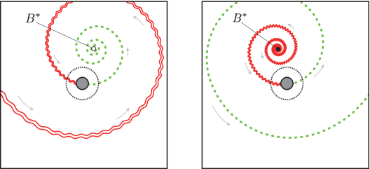
Figure 7: The image of the Julia set (red) by $\Phi_{t}$ in $W$-coordinate for Cases 1 and 2⁺ (left) and Case 2^- (right). The origin of the $W$-plane is the center of the dotted (or black) circle. The radius of the black circle equals $\hat{r}$. The annulus between the dotted circle and the black one encloses the region where the dynamics by $G$ is relatively close to the translation $W\mapsto W+1$ (see Proposition 10.1).

Dynamics of $G$ near infinity.

Let

$$d_{0}:=\frac{\cos A_{0}}{4}>0,$$

where $A_{0}\in[0,\pi/2)$ is given in the definition of $\Delta$ (hence it is determined by the given thickness of the thick internal ray).

Proposition 9.1.

When $|W|>1/(qd_{0}|t|)$, we have

$$|G(W)| <|W|\quad\text{in Cases 1 and 2${}^{+}$, and}$$

$$|G(W)| >|W|\quad\text{in Case 2${}^{-}$}$$

by taking sufficiently small $\hat{R}$ and $T_{0}$ in the definitions of $\hat{U}$ and $\Delta$.

Proof.

Since $G(W)/W=\tau+W^{-1}+O(W^{-2})=1\mp qt+O(t^{2})+W^{-1}+O(W^{-2})$, we have

$$\log{\left|\frac{G(W)}{W}\right|}={\mathrm{Re}\,}\log\frac{G(W)}{W}={\mathrm{Re}\,}{\left(\mp qt+O(t^{2})+W^{-1}+O(W^{-2})\right)}.$$

Now suppose that $|W|>1/(qd_{0}|t|)$. By taking a smaller $T_{0}$ if necessary, for any $t\in\Delta=\Delta(A_{0},T_{0})$ we have

$${\mathrm{Re}\,}(qt)\geq q|t|\cos A_{0}=4qd_{0}|t|,$$

$${\mathrm{Re}\,}(W^{-1})\leq|W^{-1}|\leq qd_{0}|t|,\quad\text{and}\quad{\mathrm{Re}\,}\left(O(t^{2})+O(W^{-2})\right)\leq qd_{0}|t|.$$

Hence

$$\log{\left|\frac{G(W)}{W}\right|}\leq(-4+1+1)qd_{0}|t|<0$$

in Cases 1 and 2⁺, and

$$\log{\left|\frac{G(W)}{W}\right|}\geq(4-1-1)qd_{0}|t|>0$$

in Case 2^-. $\blacksquare$

We first prove Proposition 2.4 for Case 2^-, then prove it for Case 1 and Case 2⁺.

Proof of Proposition 2.4: Case 2^-.

In this case $\tau=1+qt+O(t^{2})$ and thus $B=-1/(qt)+O(1)$. Note that we may assume $|B|>7\hat{r}$ for any $t\in\Delta$ by taking a smaller $T_{0}$ if necessary. We first claim:

Proposition 9.2.

In Case 2^-, for any $W$ with $|W|\geq\hat{r}$ and $|W-B|\geq|B|/2$, we have

$$|G(W)-B|\geq|W-B|+d_{0}$$

by taking sufficiently small $\hat{R}$ and $T_{0}$ in the definitions of $\hat{U}$ and $\Delta$.

Proof.

Since $G(W)-B=\tau(W-B)+O(W^{-1})$ and $|W-B|\geq|B|/2$,

$$|G(W)-B|=|\tau|\,|W-B|+|O(W^{-1})|\geq|W-B|+\frac{|\tau|-1}{2|\tau-1|}+|O(W^{-1})|.$$

Taking smaller $\hat{R}$ (hence a larger $\hat{r}$) and $T_{0}$ if necessary, we obtain

$$\frac{|\tau|-1}{2|\tau-1|}=\frac{{\mathrm{Re}\,}(qt)+O(|t^{2}|)}{2|qt+O(|t^{2}|)|}\geq\frac{q|t|\cos A_{0}\cdot(1+O(|t|))}{2q|t|\cdot(1+O(|t|))}\geq\frac{\cos A_{0}}{2}\cdot\frac{3}{4}$$

and $|O(W^{-1})|\leq(\cos A_{0})/8$. Hence

$$|G(W)-B|\geq|W-B|+{\left(\frac{3}{8}-\frac{1}{8}\right)}\cos A_{0}=|W-B|+d_{0}.$$

$\blacksquare$

Proposition 9.3.

In Case 2^-, there exists a unique linearizing coordinate $L:\mathbb{D}(B,3|B|/4)\to\mathbb{C}$ of the repelling fixed point $B^{\ast}$ of $G$ such that $L(B^{\ast})=0$, $DL(B^{\ast})=1$, and if $G(W)\in\mathbb{D}(B,3|B|/4)$,

$$L\circ G(W)=\tau^{\ast}L(W)$$

where $\tau^{\ast}=DG(B^{\ast})$.

Proof.

By the previous proposition, the disk $\mathbb{D}(B,3|B|/4)$ is compactly contained in $G(\mathbb{D}(B,3|B|/4))$. Hence the univalent branch of $G^{-1}$ on $G(\mathbb{D}(B,3|B|/4))$ is strictly contracting. By the Riemann mapping theorem and the Schwarz lemma, there exists a unique attracting fixed point of $G^{-1}$ in $\mathbb{D}(B,3|B|/4)$, which must be $B^{\ast}$. Hence there is a unique linearizing coordinate $L$ near $B^{\ast}$ that satisfies $L(B^{\ast})=0$, $DL(B^{\ast})=1$, and the relation $L\circ G^{-1}(W)=(\tau^{\ast})^{-1}L(W)$. We obtain the desired linearizing coordinate by extending $L$ to $\mathbb{D}(B,3|B|/4)$ by this relation. $\blacksquare$

Now we are ready to finish the proof of Proposition 2.4 in Case 2^-. Take any $z_{0}\in J(f_{c_{t}})\cap U_{0}$ for a given $t\in\Delta$. Let $W_{0}:=\Phi_{t}(z_{0})$ and $W_{k}:=G^{k}(W)$ for $k\geq 0$.

If $|W_{0}-B|\leq|B|/2$, Proposition 9.3 implies that $|W_{k}-B|>|B|/2$ for some $k\geq 1$ unless $W_{0}=B^{\ast}$. If $W_{0}=B^{\ast}$, then $z_{0}$ is a repelling fixed point of $f_{c}^{pq}$ in $U_{0}$. If $W_{0}\neq B^{\ast}$, by Proposition 9.2, either $|W_{k+j}-B|\geq|W_{k}-B|+jd_{0}\to\infty$ as $j\to\infty$ or $|W_{k+j}|\leq\hat{r}$ for some $j\geq 0$. The former implies that the orbit of $z_{0}$ is attracted to an attracting fixed point of $f_{c}^{pq}$ (see Proposition 9.1) and thus a contradiction. The latter implies that $z_{pq(k+j)}$ is not contained in $U_{0}$ any more. $\blacksquare$

Proof of Proposition 2.4: Cases 1 and 2⁺.

In this case $\tau=1-qt+O(t^{2})$ and thus $B=1/(qt)+O(1)$. The proof is analogous to Case 2^- and we only give an outline.

Since $G^{-1}(W)-B=\tau^{-1}(W-B)+O(W^{-1})$, we have

$$|G^{-1}(W)-B|\geq|W-B|+d_{0}$$ (9.1)

when $|W|\geq\hat{r}$ and $|W-B|\geq|B|/2$. The fixed point $B^{\ast}$ of $G^{-1}$ is repelling and we can find a linearizing coordinate $L$ of $G^{-1}$ in $\mathbb{D}(B,3|B|/4)$.

Let $z_{0}\in J(f_{c_{t}})\cap U_{0}$ for a given $t\in\Delta$. Let $W_{0}:=\Phi_{t}(z_{0})$ and $W_{k}:=G^{k}(W_{0})$ for $k\geq 0$. If $W_{0}=\infty$, then $z_{0}$ is the repelling fixed point of $f_{c_{t}}^{pq}$ (see Proposition 9.1). Suppose that $W_{0}\neq\infty$. Then $W_{0}$ is not contained in $\mathbb{D}(B,|B|/2)$, otherwise $W_{k}$ tends to $B^{\ast}$ as $k\to\infty$. By (9.1), we have $|W_{0}-B|\geq|W_{k}-B|+kd_{0}$ and thus either $|W_{k}-B|<3|B|/4$ or $|W_{k}|\leq\hat{r}$ for some $k\geq 0$. The former implies that $z_{pqk}$ is contained in the attracting basin of an attracting fixed point of $f_{c}^{pq}$, and thus a contradiction. The latter implies that $z_{pqk}$ is not contained in $U_{0}$ any more. $\blacksquare$

10 Proof of Lemma H

In this section we give a proof of Lemma H. The proof employs the branched coordinates and the dynamics of the form $G(W)=\tau W+1+O(1/W)$ as in the previous section.

Dynamics of $G$ near the origin.

Since $\tau\to 1$ as $t\in\Delta$ tends to $0$, the dynamics of $G$ (relatively) near the origin becomes closer to the translation $W\mapsto W+1$:

Proposition 10.1.

For any $t\in\Delta$ and any $W$ with $\hat{r}\leq|W|\leq 1/(5q|t|)$, we have $|G(W)-(W+1)|\leq 1/2$ by taking sufficiently small $\hat{R}$ and $T_{0}$ in the definitions of $\hat{U}$ and $\Delta$. In particular, we have

$$1/2\leq{\mathrm{Re}\,}G(W)-{\mathrm{Re}\,}W\leq 3/2\quad\text{and}\quad|\arg(W-G(W))|\leq\pi/6.$$ (10.1)

Proof.

We have $|(\tau-1)W|=|(\mp qt+O(t^{2}))W|\leq 1/4$ when $|W|\leq(5q|t|)^{-1}$ by taking a smaller $T_{0}$. We also have $|G(W)-(\tau W+1)|=|O(1/W)|\leq 1/4$ when $|W|\geq\hat{r}$ by taking a smaller $\hat{R}$ (hence a larger $\hat{r}$). It follows that $|G(W)-(W+1)|=|(\tau-1)W+O(1/W)|\leq 1/2$ and (10.1) is an immediate consequence. $\blacksquare$

Some additional conditions on $U_{0}$ in $W$-coordinate.

In what follows we suppose that $z_{0}\in J(f_{c_{t}})\cap U_{0}$, and there exists an $m\in\mathbb{N}$ such that $z_{(m-1)pq}\in U_{0}$ but $z_{mpq}\notin U_{0}$. Let $W_{k}:=\Phi_{t}(z_{kpq})$. Then we may assume that $W_{m-1}\in\Phi_{t}(U_{0})$ but $W_{m}\notin\Phi_{t}(U_{0})$.

By taking smaller and appropriate $\hat{R}$ and $R_{0}$ in the definitions of $\hat{U}$ and $U_{0}$ (and taking a smaller $T_{0}$ if necessary), we may assume that the set $\Phi_{t}(\partial U_{0})$ is contained in the annulus

$$\hat{A}:={\left\{W\in\overline{\mathbb{C}}_{W}\,:\,5\hat{r}<|W|<6\hat{r}\right\}}$$

(where $\hat{r}\asymp\hat{R}^{-q}$ is introduced in the previous section) for any $t\in\Delta$. Indeed, we can apply the Koebe distortion theorem to the family of local coordinates $\{\psi_{t}\}$ to control the shape (eccentricity) of the image $\Phi_{t}(\partial U_{0})$. Because ${\mathrm{Re}\,}W_{m}-{\mathrm{Re}\,}W_{m-1}\leq 3/2$ by Proposition 10.1, we may assume in addition that $W_{m}$ is contained in this $\hat{A}$.

Now we claim that $3\pi/4\leq\arg W_{m}\leq 5\pi/4$, equivalently, $|\arg(-W_{m})|\leq\pi/4$. Indeed, since $z_{0}$ is contained in the Julia set, the same argument as Proposition 2.4 yields that the orbit of $W_{0}$ by $G$ must leave the domain of $G$ (by taking a larger $\hat{r}$ if necessary). In other words, there exists an integer $k>m$ such that $|W_{k}|>\hat{r}$ and $|W_{k+1}|\leq\hat{r}$. Since $|\arg(W_{k}-W_{m})|\leq\pi/6$ by the proposition above, the condition $|W_{m}|>5\hat{r}$ implies $|\arg(-W_{m})|\leq\pi/4$. (Here we have used $\cos(5\pi/12)>1/5$. See Figure 8.)

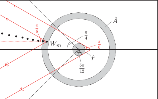
Figure 8: The orbit leaving the domain $\Phi_{t}(U_{0})$ of $G$.

The lemma below is a very important conclusion from the radial access condition:

Lemma I.

There exists a constant $K_{\mathrm{I}}\in(0,1/(5q)]$ such that for any $t\in\Delta$, $z_{0}\in J(f_{c_{t}})\cap U_{0}$ and $k\geq 0$, the condition $|W_{k}|\leq K_{\mathrm{I}}/|t|$ implies $|\arg(-W_{k})|\leq\pi/4$. Moreover, for such a $W_{k}$, we have $|W_{k+1}|<|W_{k}|$.

Hence we can only find $W_{k}$ near the negative real axis in the disk $\mathbb{D}(0,K_{\mathrm{I}}/|t|)$.

Proof.

By the assumption on $|W_{m}|$ as above, we may assume that there exists $j\in\mathbb{N}$ such that

$$W_{m-j},\,W_{m-j+1},\cdots,W_{m}\in{\left\{W\in\overline{\mathbb{C}}_{W}\,:\,|W|\leq(5q|t|)^{-1},\,|\arg(-W)|\leq\pi/4\right\}}$$

and that $|W_{m-j}|\geq(6q|t|)^{-1}$. Note that the condition $|\arg(-W)|\leq\pi/4$ implies $|W|/\sqrt{2}\leq-{\mathrm{Re}\,}W\leq|W|.$

By Proposition 10.1, we have ${\mathrm{Re}\,}W_{m}-{\mathrm{Re}\,}W_{m-j}\leq 3j/2$ and thus

$$3j/2\geq-|W_{m}|+|W_{m-j}|/\sqrt{2}\geq-|W_{m}|+(6\sqrt{2}q|t|)^{-1}.$$

Since the assumption $5\hat{r}<|W_{m}|<6\hat{r}$ implies $|W_{m}|\asymp 1$, we conclude that $j\geq C_{6}/|t|$ for some constant $C_{6}\asymp 1$ independent of $t\in\Delta$ (taking a smaller $T_{0}$ if necessary).

In Case 2^-, as in the proof of Proposition 2.4, there is $k^{\prime}>j\geq 1$ for which $|W_{m-k^{\prime}}-B|>|B|/2$ (otherwise $W_{0}=B^{*}$). We have

$$|W_{m}-B|\geq|W_{m-k^{\prime}}-B|+k^{\prime}d_{0}>|W_{m-k^{\prime}}-B|+C_{6}d_{0}/|t|$$

by Proposition 9.2. Hence

$$|W_{m-k^{\prime}}|\geq|B|-|W_{m-k^{\prime}}-B|>|B|-|W_{m}-B|+C_{6}d_{0}/|t|\geq-|W_{m}|+C_{6}d_{0}/|t|.$$

Since $|W_{m}|\asymp 1$, there exists a constant $K_{\mathrm{I}}\asymp 1$ such that $|W_{m-k^{\prime}}|>K_{\mathrm{I}}/|t|$ for any such $k^{\prime}$ and $t\in\Delta$ (again taking a smaller $T_{0}$ if necessary). Hence if we have $|W_{k}|\leq K_{\mathrm{I}}/|t|$ for some $k$, then $m-j\leq k\leq m$ and thus $|\arg(-W_{k})|\leq\pi/4$. Since $|W_{k}|\leq K_{\mathrm{I}}/|t|$ also implies $|W_{k}|\leq 1/(5q|t|)$, we conclude $K_{\mathrm{I}}\leq 1/(5q)$.

The proof for Cases 1 and 2⁺ is analogous: By (9.1), we have

$$|W_{m-k^{\prime}}-B|\geq|W_{m}-B|+k^{\prime}d_{0}>|W_{m}-B|+C_{6}d_{0}/|t|$$

instead, and this implies

$$|W_{m-k^{\prime}}|\geq|W_{m-k^{\prime}}-B|-|B|>|W_{m}-B|-|B|+C_{6}d_{0}/|t|\geq-|W_{m}|+C_{6}d_{0}/|t|.$$

Then we repeat the same argument as above.

Now, we show the condition $|W_{k}|\leq K_{\mathrm{I}}/|t|$ implies $|W_{k+1}|<|W_{k}|$. By Proposition 10.1, we get $|W_{k+1}-(W_{k}+1)|\leq 1/2$ and thus

$$\left|\frac{W_{k+1}}{W_{k}}\right|\leq\left|1+\frac{1}{W_{k}}\right|+\frac{1}{2|W_{k}|}.$$

Since $|\arg(-W_{k})|\leq\pi/4$ implies $3\pi/4\leq\arg(1/W_{k})\leq 5\pi/4$, we obtain

$$\left|1+\frac{1}{W_{k}}\right|\leq\sqrt{{\left(1-\frac{1}{\sqrt{2}~{}|W_{k}|}\right)}^{2}+{\left(\frac{1}{\sqrt{2}~{}|W_{k}|}\right)}^{2}}$$

and thus

$$\left|\frac{W_{k+1}}{W_{k}}\right| \leq 1-\frac{1}{\sqrt{2}~{}W_{k}}+\frac{1}{2~{}|W_{k}|}+O\left(\frac{1}{|W_{k}|^{2}}\right)$$

$$= 1-\frac{\sqrt{2}-1}{2~{}|W_{k}|}+O\left(\frac{1}{|W_{k}|^{2}}\right)$$

$$< 1$$

by taking a sufficiently large $\hat{r}$ if necessary. $\blacksquare$

Remark 10.2.

Once we have $|W_{k}|\leq K_{\mathrm{I}}/|t|$, then $|W_{j}|\leq K_{\mathrm{I}}/|t|$ for $k\leq j\leq m$.

Proposition 10.3.

For any $t\in\Delta$, any $z_{0}\in J(f_{c_{t}})\cap U_{0}$ that is not a fixed point of $f_{c_{t}}^{pq}$, and any $k$ with $0\leq k\leq m$, we have

$$|DG^{k}(W_{0})|\asymp|\tau|^{k}$$

in Case 1 or Case 2⁺, and

$$|DG^{k}(W_{0})|\asymp|\tau^{\ast}|^{k}$$

in Case 2^-, where $W_{0}=\Phi_{t}(z_{0})$. The implicit constants are independent of $t,z_{0}$, and $k$.

Proof for Case 1 and Case 2⁺.

Since $DG(W)=\tau+O(W^{-2})$,

$$DG^{k}(W_{0})=\tau^{k}\,\prod_{j=0}^{k-1}{\left(1+O({W_{j}}^{-2})\right)}.$$ (10.2)

Hence it is enough to show that $\sum_{j=0}^{k-1}|W_{j}|^{-2}$ is uniformly bounded in $t$, $W_{0}$, and $k$.

As in the proof of Proposition 2.4, $\mathbb{D}(B,3|B|/4)$ is contained in the attracting basin of $B^{*}$. Therefore, we may always assume $|W_{j}|\geq\hat{r}$ and $|W_{j}-B|>|B|/2$ for $j=0,1,\ldots,k$. By (9.1), $|W_{j}-B|$ is strictly decreasing in $j$. This implies that if $|W_{k_{1}}-B|<4|B|$ for some $0\leq k_{1}\leq k$, then $|W_{j}-B|<4|B|$ for all $k_{1}\leq j\leq k$. On the other hand, by Lemma I, if $|W_{k_{2}}|\leq K_{\mathrm{I}}/|t|$ for some $0\leq k_{2}\leq k$, then $|W_{j}|\leq K_{\mathrm{I}}/|t|$ and $|\arg(-W_{j})|\leq\pi/4$ for all $k_{2}\leq j\leq k$ $(\leq m)$. Consequently, we can assume the location of $W_{0},\ldots,W_{k}$ to be

1. $|W_{j}-B|\geq 4|B|$ for $j=0,\ldots,k_{1}-1$,

2. $|W_{j}-B|<4|B|$ and $|W_{j}|>K_{\mathrm{I}}/|t|$ for $j=k_{1},\ldots,k_{2}-1$,

3. $|W_{j}-B|<4|B|$ and $|W_{j}|\leq K_{\mathrm{I}}/|t|$ for $j=k_{2},\ldots,k$.

For the case (i⁺), by (9.1) again we have

$$|W_{j}|\geq|W_{j}-B|-|B|\geq|W_{k_{1}-1}-B|-|B|+(k_{1}-1-j)d_{0}\geq|B|+(k_{1}-1-j)d_{0}.$$

Hence

$$\sum_{j=0}^{k_{1}-1}|W_{j}|^{-2}=O{\left(\sum_{j=0}^{k_{1}-2}\frac{1}{(k_{1}-1-j)^{2}}\right)}+\frac{1}{|B|^{2}}=O{\left(\sum_{j=1}^{\infty}\frac{1}{j^{2}}\right)}+O{\left(|t|^{2}\right)}=O(1).$$

The condition $|W_{j}-B|<4|B|$ implies $|W_{j}|<5|B|=5/(q|t|)+O(1)$. Hence the case (ii⁺) implies $|W_{j}|\asymp|t|^{-1}$ and thus $|W_{j}|^{-2}\asymp|t|^{2}$. From (9.1), we obtain

$$4|B|>|W_{k_{1}}-B|\geq|W_{k_{2}-1}-B|+(k_{2}-1-k_{1})d_{0}\geq(k_{2}-1-k_{1})d_{0}$$

and thus $k_{2}-1-k_{1}=O(|t|^{-1})$. This gives

$$\sum_{j=k_{1}}^{k_{2}-1}|W_{j}|^{-2}=O(|t|).$$

In the (iii⁺) case, we have $|\arg(-W_{j})|\leq\pi/4$ and thus $|W_{j}|/\sqrt{2}\leq-{\mathrm{Re}\,}W_{j}\leq|W_{j}|$. By Proposition 10.1, we have $-{\mathrm{Re}\,}W_{j}\geq-{\mathrm{Re}\,}W_{k}+(k-j)/2.$ Hence, we get $|W_{j}|\geq|W_{k}|/\sqrt{2}+(k-j)/2\geq(k-j)/2$, and

$$\sum_{j=k_{2}}^{k-1}|W_{j}|^{-2}=O{\left(\sum_{j=k_{2}}^{k-1}\frac{1}{(k-j)^{2}}\right)}=O{\left(\sum_{j=1}^{\infty}\frac{1}{j^{2}}\right)}=O(1).$$

Proof for Case 2^-.

First note by Proposition 9.1 that $|W_{j}|\leq 1/(qd_{0}|t|)$ for $0\leq j\leq k$ (otherwise $W_{j}$ must be attracted by $\infty$). Second, by Proposition 9.2, if $|W_{k_{1}}-B|\geq|B|/2$ for some least $k_{1}\leq k$, then $|W_{j}-B|$ is strictly increasing for $j$ with $k_{1}\leq j\leq k$. Hence, $|W_{j}-B|\geq|B|/2$ for such a $j$. Furthermore, if $|W_{k_{2}}|\leq K_{\mathrm{I}}/|t|$ for some $0\leq k_{2}\leq k$, then as in the Case 1 and Case 2⁺, the location of $W_{0},\ldots,W_{k}$ must be

1. $|W_{j}-B|<|B|/2$ for $j=0,\ldots,k_{1}-1$,

2. $|W_{j}-B|\geq|B|/2$ and $|W_{j}|>K_{\mathrm{I}}/|t|$ for $j=k_{1},\ldots,k_{2}-1$,

3. $|W_{j}-B|\geq|B|/2$ and $|W_{j}|\leq K_{\mathrm{I}}/|t|$ for $j=k_{2},\ldots,k$.

Now,

$$\frac{DG^{k}(W_{0})}{(\tau^{\ast})^{k}}$$

$$= \frac{DG^{k_{1}-1}(W_{0})}{(\tau^{\ast})^{k_{1}-1}}\cdot\frac{DG^{k-k_{1}+1}(W_{k_{1}-1})}{(\tau^{\ast})^{k-k_{1}+1}}$$

$$\asymp 1\cdot\frac{DG^{k-k_{1}+1}(W_{k_{1}-1})}{(\tau^{\ast})^{k-k_{1}+1}}\qquad\mbox{(by Proposition \ref{prop_2-_2})}$$

$$\asymp {\left(\frac{\tau}{\tau^{\ast}}\right)}^{k-k_{1}+1}\prod_{j=k_{1}-1}^{k-1}{\left(1+O({W_{j}}^{-2})\right)}\qquad\mbox{(as \eqref{DGk=})}$$

$$\asymp {\left(1+O(t^{2})\right)}^{k-k_{1}+1}\cdot\prod_{j=k_{1}-1}^{k-1}{\left(1+O({W_{j}}^{-2})\right)}\qquad\mbox{(since $\displaystyle\frac{\tau}{\tau^{\ast}}=1+O(t^{2})$.)}$$

Because $|W_{k_{1}-1}|\geq|B|-|W_{k_{1}-1}-B|>|B|-|B|/2=|B|/2=O(1/|t|)$ and because $|W_{k_{1}-1}|\leq 1/(qd_{0}|t|)$, we have $|W_{k_{1}-1}^{-2}|=O(|t|^{2})$.

By Proposition 9.2, we know

$$|W_{k}-B|\geq|W_{k_{1}}-B|+(k-k_{1})d_{0}\geq(k-k_{1})d_{0}$$

and thus $k-k_{1}\leq(|W_{k}|+|B|)/d_{0}=O(|t|^{-1})$. This implies that $(1+O(t^{2}))^{k-k_{1}+2}=1+O(t)$.

It remains to obtain an estimate of $\prod_{j=k_{1}}^{k-1}{\left(1+O(W_{j}^{-2})\right)}$. Again, it is enough to obtain an estimate by showing that $\sum_{j=k_{1}}^{k-1}|W_{j}|^{-2}$ is uniformly bounded in $k$ and $W_{0}$.

For the (ii^-) case, since $|W_{j}|<1/(qd_{0}|t|)$, we obtain $|W_{j}|\asymp|t|^{-1}$. Therefore,

$$\sum_{j=k_{1}}^{k_{2}-1}|W_{j}|^{-2}=O(|t|)\qquad\mbox{(since $k-k_{1}=O(|t|^{-1})$ so is $k_{2}-k_{1}$.)}$$

The (iii^-) case follows exactly as the (iii⁺) case.

The proof of Proposition 10.3 is complete. $\blacksquare$

Lemma H in the branched coordinates.

To give estimates for the sums of the form

$$\sum_{k=0}^{m-1}\frac{1}{|Df_{c}^{kpq}(z_{j})|}\quad\text{and}\quad\sum_{k=0}^{m-1}\frac{|c-{\hat{c}}|+|f_{c}^{kpq}(z_{j})-b_{j}(c)|}{|Df_{c}^{kpq}(z_{j})|}$$

with $0\leq j\leq p-1$, we rewrite them in $W$-coordinates. It is enough to consider the case of $j=0$, since we may apply the same argument as in the proof of Lemma G.

Let $W=\Phi_{t}(z)=\Psi_{t}\circ\psi_{t}(z)$ for $z\in\hat{U}$ such that $W_{k}:=\Phi_{t}(z_{kpq})$ for each $k$. Note that $|D\psi_{t}(z)|\asymp 1$ for any $z\in\hat{U}$, where the implicit constant is independent of $t\in\Delta$. Since $D\Psi_{t}(w)=\lambda_{t}^{q^{2}}/w^{q+1}$, we have

$$|D\Phi_{t}(z)|=|D\Psi_{t}(w)\cdot D\psi_{t}(z)|\asymp|w|^{-(q+1)}\asymp|W|^{1+1/q}.$$

By the chain rule, we obtain

$$|Df_{c_{t}}^{kpq}(z_{0})| =|D(\Phi_{t}^{-1}\circ G^{k}\circ\Phi_{t})(z_{0})|=|D\Phi_{t}^{-1}(W_{k})\cdot DG^{k}(W_{0})\cdot D\Phi_{t}(z_{0})|$$

$$\asymp|W_{k}|^{-1-1/q}\cdot|DG^{k}(W_{0})|\cdot|W_{0}|^{1+1/q}$$

$$={\left|\frac{W_{0}}{W_{k}}\right|}^{1+1/q}\cdot|DG^{k}(W_{0})|.$$

We let

$${\mathcal{S}}_{1}:=\sum_{k=0}^{m-1}{\left|\frac{W_{k}}{W_{0}}\right|}^{1+1/q}\cdot\frac{1}{|DG^{k}(W_{0})|}\asymp\sum_{k=0}^{m-1}\frac{1}{|Df_{c_{t}}^{kpq}(z_{0})|},$$

and

$${\mathcal{S}}_{2}:=\frac{1}{|W_{0}|^{1/q}}\sum_{k=0}^{m-1}{\left|\frac{W_{k}}{W_{0}}\right|}\cdot\frac{1}{|DG^{k}(W_{0})|}\asymp\sum_{k=0}^{m-1}\frac{|f_{c_{t}}^{kpq}(z_{0})-b_{t}|}{|Df_{c_{t}}^{kpq}(z_{0})|},$$

where we used the fact that $|f_{c}^{kpq}(z_{0})-b_{0}(c)|=|z_{kpq}-b_{t}|\asymp|W_{k}|^{-1/q}$. Now Lemma H is reduced to the estimates

$${\mathcal{S}}_{1}=O{\left(\frac{1}{|t|}\right)}\quad\text{and}\quad{\mathcal{S}}_{2}=O{\left(\frac{1}{|t|^{1-1/q}}\right)}.$$

Indeed, Proposition 2.2 implies

$$\sum_{k=0}^{m-1}\frac{1}{|Df_{c_{t}}^{kpq}(z_{0})|}\asymp{\mathcal{S}}_{1}=O{\left(\frac{1}{|t|}\right)}=O{\left(\frac{1}{\sqrt{|c_{t}-{\hat{c}}|}}\right)}$$

in Case 1, and

$$\sum_{k=0}^{m-1}\frac{|c_{t}-{\hat{c}}|+|f_{c_{t}}^{kpq}(z_{0})-b_{t}|}{|Df_{c_{t}}^{kpq}(z_{0})|} \asymp|c_{t}-{\hat{c}}|{\mathcal{S}}_{1}+{\mathcal{S}}_{2}$$

$$=O{\left(|t|\cdot\frac{1}{|t|}+\frac{1}{|t|^{1-1/q}}\right)}=O{\left(\frac{1}{|c_{t}-{\hat{c}}|^{1-1/q}}\right)}$$

in Case 2.

Proof of Lemma H for Case $2^{-}$.

We will use tha fact that $\tau^{\ast}=1+qt+O(t^{2})$ and

$$|\tau^{\ast}|=1+{\mathrm{Re}\,}(qt)+O(|t^{2}|)\geq 1+qd_{0}|t|$$

for $t\in\Delta$ if we take a smaller $T_{0}$ if necessary.

First, suppose that $|W_{0}|\geq K_{\mathrm{I}}/|t|$. Since it must be $|W_{k}|\leq 1/(qd_{0}|t|)$ for any $k=0,1,\ldots,m$ by Proposition 9.1 (otherwise $W_{k}$ is attracted by $\infty$), we have $|W_{0}|\asymp|t|^{-1}$ and $|W_{k}/W_{0}|=O(1)$. Hence by Proposition 10.3, we have

$${\mathcal{S}}_{1}=\sum_{k=0}^{m-1}{\left|\frac{W_{k}}{W_{0}}\right|}^{1+1/q}\cdot\frac{1}{|DG^{k}(W_{0})|}=\sum_{k=0}^{m-1}O(1)\cdot\frac{1}{|\tau^{\ast}|^{k}}=O{\left(\sum_{k=0}^{m-1}\frac{1}{(1+qd_{0}|t|)^{k}}\right)}=O{\left(\frac{1}{|t|}\right)}$$

and

$${\mathcal{S}}_{2}=\frac{1}{|W_{0}|^{1/q}}\sum_{k=0}^{m-1}{\left|\frac{W_{k}}{W_{0}}\right|}\cdot\frac{1}{|DG^{k}(W_{0})|}=|t|^{1/q}\sum_{k=0}^{m-1}O(1)\cdot\frac{1}{|\tau^{\ast}|^{k}}=O{\left(\frac{1}{|t|^{1-1/q}}\right)}.$$

Next, suppose that $|W_{0}|\leq K_{\mathrm{I}}/|t|$. By Proposition 10.1 and Lemma I, we have $|\arg(-W_{k})|\leq\pi/4$ and thus $|W_{k}|/\sqrt{2}\leq-{\mathrm{Re}\,}W_{k}\leq|W_{k}|$ for any $k=0,1,\ldots,m$. By Proposition 10.1 again we have ${\mathrm{Re}\,}W_{0}+k/2\leq{\mathrm{Re}\,}W_{k}$. Hence

$$0\leq|W_{k}|/\sqrt{2}\leq-{\mathrm{Re}\,}W_{k}\leq-{\mathrm{Re}\,}W_{0}-k/2\leq|W_{0}|-k/2$$ (10.3)

and this implies

$${\left|\frac{W_{k}}{W_{0}}\right|}\leq\sqrt{2}\cdot\frac{|W_{0}|-k/2}{|W_{0}|}=O(1).$$

In particular, by letting $k=m$ in (10.3) we have $m\leq 2|W_{0}|=O(|W_{0}|)$.

Since $|W_{0}|\leq K_{\mathrm{I}}/|t|$, we have

$${\mathcal{S}}_{1}=\sum_{k=0}^{m-1}O(1)\cdot\frac{1}{|\tau^{\ast}|^{k}}\leq\sum_{k=0}^{m-1}O(1)\cdot 1^{k}=O(m)=O(|W_{0}|)=O{\left(\frac{1}{|t|}\right)}$$

and

$${\mathcal{S}}_{2} =\frac{1}{|W_{0}|^{1/q}}\sum_{k=0}^{m-1}O(1)\cdot\frac{1}{|\tau^{\ast}|^{k}}\leq\frac{1}{|W_{0}|^{1/q}}\sum_{k=0}^{m-1}O(1)\cdot 1^{k}$$

$$=\frac{O(m)}{|W_{0}|^{1/q}}=O(|\,W_{0}|^{1-1/q}|)=O{\left(\frac{1}{|t|^{1-1/q}}\right)}.$$

This completes the proof for Case 2^-.

Preliminary for Case 1 and Case $2^{+}$.

We will use the fact that $\tau^{-1}=1+qt+O(t^{2})$ and

$$|\tau|^{-1}=1+{\mathrm{Re}\,}(qt)+O(|t^{2}|)\geq 1+qd_{0}|t|$$

for $t\in\Delta$ if we take a smaller $T_{0}$ if necessary.

It is very convenient to use Ueda’s modulus defined as follows (see [U]): For $W\neq\infty$,

$$N(W):=|W-B|-|B|.$$

Then one can easily check that

• $|W|\geq N(W)$; and

• $N(W)\geq|W|/3$ when $|W-B|\geq 4|B|$.

Indeed, $|W|\geq N(W)$ is just the triangle inequality; and when $|W-B|\geq 4|B|$, we have $|W|\geq 3|B|$ and thus $N(W)/|W|=|1-B/W|-|B/W|\geq 1/3$.

Here is another useful fact:

Proposition 10.4.

In Case 1 and Case 2⁺, we have

$$N(G^{-1}(W))\geq|\tau|^{-1}N(W)+d_{0}$$

by taking sufficiently small $\hat{R}$ and $T_{0}$ in the definitions of $\hat{U}$ and $\Delta$.

Proof.

Since $|G^{-1}(W)-B|=|\tau|^{-1}|W-B|+O(|W^{-1}|)$, we have

$$N(G^{-1}(W))=|\tau|^{-1}N(W)+\frac{|\tau|^{-1}-1}{|1-\tau|}+O(|W^{-1}|).$$

By taking a smaller $T_{0}$ if necessary, we have

$$\frac{|\tau|^{-1}-1}{|1-\tau|}=\frac{{\mathrm{Re}\,}t}{|t|}(1+O(|t|))\geq\frac{\cos A_{0}}{2}=2d_{0}$$

for any $t\in\Delta$. By taking a smaller $\hat{R}$ (hence a larger $\hat{r}$) if necessary, we have $O(|W^{-1}|)\leq(\cos A_{0})/4=d_{0}$ for any $|W|\geq\hat{r}$. Hence we have the desired inequality. $\blacksquare$

Proposition 10.5.

In Case 1 and Case 2⁺, we have

$${\left|\frac{W_{k}}{W_{0}}\right|}=O(|\tau|^{k})$$

for any $k=0,1,\ldots,m$.

Proof.

We adopt the argument of Proposition 10.3 and assume that

1. $|W_{j}-B|\geq 4|B|$ for $j=0,\ldots,k_{1}-1$,

2. $|W_{j}-B|<4|B|$ and $|W_{j}|>K_{\mathrm{I}}/|t|$ for $j=k_{1},\ldots,k_{2}-1$,

3. $|W_{j}-B|<4|B|$ and $|W_{j}|\leq K_{\mathrm{I}}/|t|$ for $j=k_{2},\ldots,k$

for some $k_{1}$ and $k_{2}$. Now we consider the product

$${\left|\frac{W_{k}}{W_{0}}\right|}={\left|\frac{W_{k_{1}-1}}{W_{0}}\right|}\cdot{\left|\frac{W_{k_{2}}}{W_{k_{1}-1}}\right|}\cdot{\left|\frac{W_{k}}{W_{k_{2}}}\right|}.$$ (10.4)

In the case of (i⁺), we can apply Proposition 10.4 and it follows that

$$|W_{0}|\geq N(W_{0})\geq|\tau|^{-(k_{1}-1)}N(W_{k_{1}-1})\geq|\tau|^{-k_{1}+1}|W_{k_{1}-1}|/3.$$

Hence $|W_{k_{1}-1}/W_{0}|\leq 3\,|\tau|^{k_{1}-1}$. Since $|W_{k_{1}-1}|\geq 3|B|=3/(q|t|)+O(1)$ and $|W_{k_{2}}|\leq K_{\mathrm{I}}/|t|$, we have $|W_{k_{2}}/W_{k_{1}-1}|=O(1)$. Since $|W_{j}|$ is decreasing in the case of (iii⁺) by Lemma I, we have $|W_{k}/W_{k_{2}}|\leq 1$. Hence by (10.4), we obtain $|W_{k}/W_{0}|=O(|\tau|^{k_{1}-1})$.

To show the estimate $|W_{k}/W_{0}|=O(|\tau|^{k})$, it is enough to show that $|\tau|^{k-(k_{1}-1)}=O(1)$. Because $|W_{k_{1}}-B|\leq 4|B|$ and hence $|W_{k_{1}}|\leq 5|B|$, by (9.1) we have

$$|W_{k_{1}}-B|\geq|W_{k}-B|+(k-k_{1})\,d_{0}\geq(k-k_{1})\,d_{0}$$

and thus $k-k_{1}\leq(|W_{k_{1}}|+|B|)/d_{0}=O(|t|^{-1})$. Hence

$$|\tau|^{k-(k_{1}-1)}=(1-{\mathrm{Re}\,}(qt)+O(t^{2}))^{k-k_{1}}\cdot|\tau|=O(1)$$

and this completes the proof. $\blacksquare$

Proof of Lemma H for Case 1 and Case $2^{+}$.

By Propositions 10.3 and 10.5, we have

$${\mathcal{S}}_{1}=\sum_{k=0}^{m-1}{\left|\frac{W_{k}}{W_{0}}\right|}^{1+1/q}\cdot\frac{1}{|DG^{k}(W_{0})|}=\sum_{k=0}^{m-1}O(|\tau|^{k(1+1/q)})\cdot\frac{1}{|\tau|^{k}}=O{\left(\sum_{k=0}^{m-1}|\tau|^{k/q}\right)}.$$

Since $|\tau|^{1/q}\leq 1-d_{0}|t|$ for $t\in\Delta$ (by taking a smaller $T_{0}$ if necessary), we obtain ${\mathcal{S}}_{1}=O(|t|^{-1})$.

Similarly we have

$${\mathcal{S}}_{2}=\frac{1}{|W_{0}|^{1/q}}\sum_{k=0}^{m-1}{\left|\frac{W_{k}}{W_{0}}\right|}\cdot\frac{1}{|DG^{k}(W_{0})|}=\frac{1}{|W_{0}|^{1/q}}\sum_{k=0}^{m-1}O(|\tau|^{k})\cdot\frac{1}{|\tau|^{k}}=\frac{O(m)}{|W_{0}|^{1/q}}.$$

First we suppose that $|W_{0}-B|<4|B|$. Then we have $|W_{0}|<5|B|=O(|t|^{-1})$. By (9.1),

$$|W_{0}|\geq|W_{0}-B|-|B|\geq|W_{m}-B|-|B|+md_{0}\geq-|W_{m}|+md_{0}.$$

By the assumption that $W_{m}\in\hat{A}$, we have $|W_{m}|<6\hat{r}$ and thus $md_{0}\leq|W_{0}|+6\hat{r}$. We obtain $m=O(|W_{0}|)$ since $5\hat{r}<|W_{0}|=O(|t|^{-1})$. Hence

$${\mathcal{S}}_{2}=\frac{O(m)}{|W_{0}|^{1/q}}=O(|W_{0}|^{1-1/q})=O{\left(\frac{1}{|t|^{1-1/q}}\right)}.$$

Next we suppose that $|W_{0}-B|\geq 4|B|$. There exists a $k\geq 0$ such that

• $|W_{j}-B|\geq 4|B|$ for $0\leq j\leq k$; and

• $|W_{j}-B|<4|B|$ for $k\leq j\leq m$.

(We may regard $k$ and $m$ as $k_{1}-1$ and $k$ in the proof of Proposition 10.5 respectively.) Since $|W_{k}/W_{0}|\leq 3|\tau|^{k}$ as in the proof of Proposition 10.5, and $|W_{k}|\geq 3|B|>1/(q|t|)$ for $t\in\Delta$, we have $3|\tau|^{k}\geq 1/(q|tW_{0}|)$. Hence

$$1<|\tau|^{-k}\leq 3q|tW_{0}|,\quad\mbox{or equivalently}\quad 0<k\log|\tau|^{-1}\leq\log(3q|tW_{0}|).$$

This implies that

$$0<k({\mathrm{Re}\,}(qt)+O(t^{2}))\leq\log(3q|tW_{0}|).$$

Since ${\mathrm{Re}\,}(qt)+O(t^{2})\geq(q|t|\cos A_{0})/2$ for $t\in\Delta$ (by taking a smaller $T_{0}$ if necessary), we conclude

$$k=O{\left(\frac{\log(3q|tW_{0}|)}{|t|}\right)}.$$

As in the proof of Proposition 10.5, we have $m-k=O(1/|t|)$. Since $|W_{0}|\geq 3|B|\geq 2/(q|t|)$ (for $t\in\Delta$ by taking a smaller $T_{0}$ if necessary), we obtain $\log(3q|tW_{0}|)\geq\log 6>1$ and thus

$$m=k+(m-k)=O{\left(\frac{\log(3q|tW_{0}|)}{|t|}\right)}+O{\left(\frac{1}{|t|}\right)}=O{\left(\frac{\log(3q|tW_{0}|)}{|t|}\right)}.$$

Hence we conclude that

$${\mathcal{S}}_{2}=\frac{O(m)}{|W_{0}|^{1/q}}=O{\left(\frac{\log(3q|tW_{0}|)}{|tW_{0}|^{1/q}}\right)}\cdot\frac{1}{|t|^{1-1/q}}=O{\left(\frac{1}{|t|^{1-1/q}}\right)},$$

where we used the fact that $x^{-1/q}\log(3qx)$ is bounded if $3qx\geq 6$. $\blacksquare$

11 Proof of Lemma D

In this section we give a proof of Lemma D. Since the proof heavily relies on Lemma I, we restate Lemma D in terms of the parameter $t\in\Delta\cup\{0\}$. (Note that we have ${\hat{c}}=c_{0}$).

Proposition 11.1.

There exist constants $K_{\mathrm{D}}>0$ and $\nu_{0}\in(0,R_{0})$ such that for any $\nu\in(0,\nu_{0})$, there exists a constant $T_{0}=T_{0}(\nu)\in(0,2\cos A_{0})$ such that for any $t\in\Delta=\Delta(A_{0},T_{0})$, $\zeta\in P(f_{c_{0}})$, and $z\in J(f_{c_{t}})-{\mathcal{V}}(c_{t})$,

$$|\zeta-z|\geq K_{\mathrm{D}}\,\nu.$$

Without loss of generality, we may assume that $K_{\mathrm{D}}\leq 1$.

Proof.

We prove it by contradiction. Suppose that for any $K_{\mathrm{D}}>0$ and $\nu_{0}\in(0,R_{0})$, there exists a $\nu\in(0,\nu_{0})$ such that for any $T_{0}\in(0,2\cos A_{0})$, there exist $t\in\Delta=\Delta(A_{0},T_{0})$, $\zeta\in P(f_{c_{0}})$, and $z\in J(f_{c_{t}})-{\mathcal{V}}(c_{t})$ such that

$$|\zeta-z|<K_{\mathrm{D}}\,\nu.$$

For instance, let $K_{\mathrm{D}}:=1/n$, $\nu_{0}:=R_{0}/n$ for integer $n\geq 1$. Then for any sufficiently large $n$, we may assume that $R_{0}/n<1$ and there exists a $\nu_{n}\in(0,R_{0}/n)$ such that for $T_{0}:=2\nu_{n}^{2q}\cos A_{0}$ we can find sequences $t_{n}\in\Delta=\Delta(A_{0},T_{0})$, $\zeta_{n}\in P(f_{c_{0}})$, and $z_{n}\in J(f_{c_{n}})-{\mathcal{V}}(c_{n})$ with $c_{n}=c_{t_{n}}$ such that

$$|\zeta_{n}-z_{n}|<\frac{1}{n}\cdot\nu_{n}.$$

(Now, $\mathcal{V}(c_{n})=\bigcup_{k=0}^{p-1}f_{c_{n}}^{-k}(V_{0})$ and $V_{0}=\mathbb{D}({\hat{b}},\nu_{n})$.) We may assume that $\zeta_{n}$ and $z_{n}$ tends to the same limit $\hat{\zeta}\in P(f_{c_{0}})$ by passing through a subsequence, since $P(f_{c_{0}})$ is compact and the Julia sets $J(f_{c_{n}})$ are uniformly bounded. Moreover, there exists a $j\geq 0$ such that $f_{c_{0}}^{j}(\hat{\zeta})$ is contained in $\mathbb{D}({\hat{b}},R_{0}/2)\subset U_{0}=\mathbb{D}({\hat{b}},R_{0})$. By replacing $\zeta_{n}$ and $z_{n}$ by $f_{c_{0}}^{j}(\zeta_{n})$ and $f_{c_{n}}^{j}(z_{n})$ respectively, we may assume that $\zeta_{n}\in U_{0}$ and $z_{n}\in U_{0}-V_{0}$ for sufficiently large $n$.

In $w$-coordinate $w=\psi_{0}(z)$ given in Proposition 2.3 for $t=0$, the local dynamics of $f_{c_{0}}^{pq}$ in $U_{0}$ can be observed as $w\mapsto w(1+w^{q}+O(w^{2q}))$ and the orbit of $\psi_{0}(\zeta_{n})$ by this map tends to $0$ tangentially to the attracting direction (that is, the set of $w$’s with ${\mathrm{Im}\,}(w^{q})=0$ and ${\mathrm{Re}\,}(w^{q})<0$). This implies that (by taking sufficiently large $j$ if necessary) $\psi_{0}(\zeta_{n})$ is contained in the set $X:=\{w\in\psi_{0}(U_{0})\,:\,|\arg(-w^{q})|\leq\pi/4\}$.

Figure 9: The sets $X$ and $Y$ in $w$-coordinate for $q=3$.

Next we consider $z_{n}\in U_{0}-V_{0}$ in the local coordinate $w=\psi_{t_{n}}(z)$. Since $\psi_{t_{n}}$ is univalent and $\nu_{n}<|z_{n}-{\hat{b}}|<R_{0}$, there exists a constant $C_{7}>0$ independent of $n$ such that $w_{n}:=\psi_{t_{n}}(z_{n})$ satisfies $|w_{n}|\geq C_{7}\nu_{n}$. In $W$-coordinate $W=\Psi_{t_{n}}(w)=-\lambda_{t_{n}}^{q^{2}}/(qw^{q})$, we have $\arg(-W)=-\arg(w^{q})+O(t_{n})$ since $\lambda_{t_{n}}^{q^{2}}=1+O(t_{n})$. Now, for $W_{n}=\Psi_{t_{n}}(w_{n})=\Psi_{t_{n}}\circ\psi_{t_{n}}(z_{n})$ with sufficiently large $n$, we obtain

$$|W_{n}|\leq\left|\frac{1+O(t_{n})}{qC_{7}^{q}\nu_{n}^{q}}\right|\leq\left|\frac{\sqrt{2\cos A_{0}}}{qC_{7}^{q}}\frac{1+O(|t_{n}|)}{\sqrt{|t_{n}|}}\right|\leq\frac{K_{\mathrm{I}}}{|t_{n}|}.$$

Therefore, by Lemma I, we have $|\arg(-W_{n})|\leq\pi/4$ since $z_{n}\in J(f_{c_{n}})\cap U_{0}$. Hence in $w$-coordinate we have $|\arg(w_{n}^{q})|=|\arg(-W_{n})|+O(|t_{n}|)\leq\pi/4+O(\nu_{n}^{2q})$ for $w_{n}=\psi_{t_{n}}(z_{n})$.

We also have $|\psi_{t_{n}}(z_{n})-\psi_{0}(z_{n})|=O(|t_{n}|)=O(\nu_{n}^{2q})$, since the map $(t,z)\mapsto\psi_{t}(z)$ is holomorphic in both $t$ and $z$. Hence $\psi_{0}(z_{n})$ is contained in $Y:=\{w\in\psi_{0}(U_{0})\,:\,|\arg(w^{q})|\leq\pi/3,\,|w|\geq C_{7}\nu_{n}\cdot(3/4)\}$ for sufficiently large $n$. It follows that $|\psi_{0}(\zeta_{n})-\psi_{0}(z_{n})|$ is larger than the distance between the sets $X$ and $Y$, which is comparable with the radius $\nu_{n}$ of $V_{0}$ (see Figure 9). However, the univalence of $\psi_{0}$ implies that $|\psi_{0}(\zeta_{n})-\psi_{0}(z_{n})|$ is not comparable with $\nu_{n}$ by $|\psi_{0}(\zeta_{n})-\psi_{0}(z_{n})|\asymp|\zeta_{n}-z_{n}|<\nu_{n}/n$. This is a contradiction. $\blacksquare$

12 Proof of Lemma C

We will show that $|Df_{c}^{M^{\prime}-M}(z_{M})|\geq\kappa_{\mathrm{C}}/\nu$ for some constant $\kappa_{\mathrm{C}}$ that does not depend on $c=c_{t}$ with $t\in\Delta$. By choosing $\nu$ sufficiently small, we have $\Lambda:=\kappa_{\mathrm{C}}/\nu>1$.

As in the proof of Lemma A, we assume that $M=0$ and $M^{\prime}=mpq+L$ for which $z_{0}\in V_{0}$ (equivalently, $|z_{0}-{\hat{b}}|<\nu$), $z_{(m-1)pq}\in U_{0}$, $z_{mpq}\notin U_{0}$ (equivalently, $|z_{mpq}-{\hat{b}}|\geq R_{0}$), and $z_{M^{\prime}}\in V_{0}$. By the chain rule we have

$$|Df_{c}^{M^{\prime}}(z_{0})|=|Df_{c}^{mpq}(z_{0})|\cdot|Df_{c}^{L}(z_{mpq})|.$$ (12.1)

First let us give an estimate of $|Df_{c}^{mpq}(z_{0})|$. For $c=c_{t}~{}(t\in\Delta)$, let $b(c)$ be the periodic point $b_{t}$ of period $p$ given in Proposition 2.3 with $b(c)\to{\hat{b}}$ as $c=c_{t}$ tends to ${\hat{c}}$. We may assume that $|b(c)-{\hat{b}}|\leq\nu$ for $c\approx{\hat{c}}$, and by the Koebe distortion Theorem, we have

$$|Df_{c}^{mpq}(z_{0})|\asymp\frac{|z_{mpq}-b(c)|}{|z_{0}-b(c)|}\geq\frac{|z_{mpq}-{\hat{b}}|-|b(c)-{\hat{b}}|}{|z_{0}-{\hat{b}}|+|b(c)-{\hat{b}}|}\geq\frac{R_{0}-\nu}{\nu+\nu}.$$

This implies that $|Df_{c}^{mpq}(z_{0})|\geq C_{8}/\nu$ for some constant $C_{8}>0$ independent of $c\approx{\hat{c}}$, $z_{0}$ and $\nu\ll 1$.

Next we give an estimate of the form $|Df_{c}^{L}(z_{mpq})|\geq C_{9}$, where $C_{9}$ is a constant independent of $c\approx{\hat{c}}$, $\nu\ll 1$, and $z_{0}\in J(f_{c})$. (Then by (12.1) the proof is done by setting $\kappa_{\mathrm{C}}:=C_{8}C_{9}$.)

As in the proof of Lemma A, by shrinking $U_{0}$ if necessary, we may always assume that $L>p$. Since $z_{M^{\prime}}\in V_{0}$, we have $z_{M^{\prime}-p}\in f_{c}^{-p}(V_{0})$ and thus $|Df_{c}^{p}(z_{M^{\prime}-p})|\geq\xi^{p}$. By Proposition 4.1 and inequality (4.1) in Lemma F we obtain

$$|Df_{c}^{L}(z_{mpq})|= |Df_{c}^{L-p}(z_{mpq})||Df_{c}^{p}(z_{M^{\prime}-p})|$$

$$\geq \frac{\rho(z_{mpq})}{\rho(z_{M^{\prime}-p})}A^{L-p}\cdot\xi^{p}$$

$$\geq \rho(z_{mpq})\cdot\mathrm{dist}\,(z_{M^{\prime}-p},P(f_{\hat{c}}))\cdot\xi^{p}.$$

Since $z_{mpq}\notin U_{0}$ and $z_{mpq}$ has a definite distance from the parabolic cycle, the distance between $z_{mpq}$ and the postcritical set $P(f_{\hat{c}})$ is larger than a positive constant independent of $c\approx{\hat{c}}$, $\nu\ll 1$, and $z_{0}\in J(f_{c})$. (Indeed, we may apply the proof of Lemma D to obtain $\mathrm{dist}\,(z_{mpq},P(f_{\hat{c}}))\geq K_{\mathrm{D}}R_{0}$ by taking a smaller $R_{0}$ if necessary.) Hence we always have $\rho(z_{mpq})\asymp 1$. Finally we show that $\mathrm{dist}\,(z_{M^{\prime}-p},P(f_{\hat{c}}))$ has a uniform distance away from zero. Since $z_{M^{\prime}}\in V_{0}$, $\mathrm{dist}\,(z_{M^{\prime}-p},P(f_{\hat{c}}))$ can be close to $0$ only if $z_{M^{\prime}-p}$ belongs to the connected component $V_{0}^{\prime}$ of $f_{c}^{-p}(V_{0})$ contained in $U_{0}$. (See Figure 6.) However, the local dynamics of $f_{c}^{p}$ on $U_{0}$ does not allow any point $z\in J(f_{c})$ satisfying both $z\in V_{0}^{\prime}-V_{0}$ and $f_{c}^{p}(z)\in V_{0}$. (More precisely, we may apply Proposition 10.1 and Lemma I to exclude such a $z$ in the Julia set.) Hence $z_{M^{\prime}-p}$ belongs to a connected component of $f_{c}^{-p}(V_{0})$ that has a definite distance from $P(f_{\hat{c}})$ and $\mathrm{dist}\,(z_{M^{\prime}-p},P(f_{\hat{c}}))$ is bounded below by a positive constant independent of $c\approx{\hat{c}}$, $\nu\ll 1$, and $z_{0}\in J(f_{c})$. In conclusion, $|Df_{c}^{L}(z_{mpq})|$ is bounded away from zero by a constant independent of $c\approx{\hat{c}}$, $\nu\ll 1$, and $z_{0}\in J(f_{c})$. $\blacksquare$

13 Proofs of Theorems 1.2 and 1.3

In this section we prove Theorem 1.2 and Theorem 1.3 together.

Proofs of Theorems 1.2 and 1.3.

Let $\sigma_{0}$ be any point in the thick internal ray ${\mathcal{I}}(\theta,\delta)$ and $\ell:=|\sigma_{0}-{\hat{c}}|$. For each $n=0,1,\ldots$, let

$$E_{n}:={\left\{c\in{\mathcal{I}}(\theta,\delta)\,:\,\frac{\ell}{2^{n+1}}\leq|c-{\hat{c}}|\leq\frac{\ell}{2^{n}}\right\}}.$$

Note that $\mathrm{diam}\,E_{n}\asymp\ell/2^{n}$ and that for any $c\in E_{n}$ we have $|c-{\hat{c}}|\asymp\ell/2^{n}$.

We take a $\sigma_{n}\in E_{n}$ for each $n\geq 1$. Then we can join $\sigma_{n}$ and $\sigma_{n+1}$ by a piecewise smooth path $\gamma_{n}$ of length compatible with $\ell/2^{n}$ contained in $E_{n}\cup E_{n+1}$. By the Main Theorem we have

$${\left|\frac{d}{dc}z(c)\right|}\leq\frac{K}{|c-{\hat{c}}|^{1-1/Q}}\asymp{\left(\frac{\ell}{2^{n}}\right)}^{-1+1/Q}$$

for any $c\in\gamma_{n}$ and $n\geq 0$. Hence

$$|z(\sigma_{n+1})-z(\sigma_{n})|={\left|\int_{\gamma_{n}}\frac{d}{dc}z(c)\,dc\right|}=O{\left({\left(\frac{\ell}{2^{n}}\right)}^{-1+1/Q}\cdot\frac{\ell}{2^{n}}\right)}=O{\left(\frac{1}{2^{n/Q}}\right)}\cdot\ell^{1/Q}.$$

It follows that the sequence $\{z(\sigma_{n})\}_{n\geq 0}$ is Cauchy, and we denote the limit by $z({\hat{c}})$. (One can easily check that the limit does not depend on the choice of the sequences $\{\sigma_{n}\}$ and $\{\gamma_{n}\}$.) Moreover, we have

$$|z(\sigma_{0})-z(\sigma_{n})|\leq O{\left(1+\frac{1}{2^{1/Q}}+\cdots+\frac{1}{2^{(n-1)/Q}}\right)}\cdot\ell^{1/Q}=O(\ell^{1/Q})$$

and thus $|z(\sigma_{0})-z({\hat{c}})|=O(\ell^{1/Q})=O(|\sigma_{0}-{\hat{c}}|^{1/Q})$, where the implicit constants depend only on ${\hat{c}}$ and the thickness $\delta$ of the thick internal ray. This proves (1.2) of Theorem 1.2.

Semiconjugacy.

Next we show that $z({\hat{c}})$ belongs to the Julia set $J(f_{\hat{c}})$. For each $z_{\ast}\in J(f_{\sigma})$ and its motion $z(c)=h_{c}(z_{\ast})=H(c,z_{\ast})$ along the thick internal ray ${\mathcal{I}}(\theta,\delta)$, we define $h_{\hat{c}}(z_{\ast})$ by the limit $z({\hat{c}})$ given as above. Since $h_{c}:J(f_{\sigma})\to J(f_{c})$ is continuous and the convergence of $h_{c}$ to $h_{\hat{c}}$ as $c\in{\mathcal{I}}(\theta,\delta)$ tends to ${\hat{c}}$ is uniform, $h_{\hat{c}}:J(f_{\sigma})\to h_{\hat{c}}(J(f_{\sigma}))$ is continuous as well. Hence by $f_{c}\circ h_{c}=h_{c}\circ f_{\sigma}$ we obtain $f_{\hat{c}}\circ h_{\hat{c}}=h_{\hat{c}}\circ f_{\sigma}$. In particular, this implies that $f_{\hat{c}}\circ h_{\hat{c}}(J(f_{\sigma}))=h_{\hat{c}}(J(f_{\sigma}))$ and thus the image $h_{\hat{c}}(J(f_{\sigma}))$ is a compact forward invariant set contained in the filled Julia set of $f_{\hat{c}}$. Suppose that there exists a $z_{\ast}\in J(f_{\sigma})$ such that $h_{\hat{c}}(z_{\ast})=z({\hat{c}})\in h_{\hat{c}}(J(f_{\sigma}))$ belongs to the Fatou set of $f_{\hat{c}}$. It actually belongs to the basin of attraction of $\hat{b}$, and thus there exists an $l$ such that $f_{{\hat{c}}}^{l+kpq}(z({\hat{c}}))$ is contained in $V_{0}$ for any $k\geq 0$. Since $h_{\hat{c}}$ is continuous, the image of any nearby point of $z_{*}$ under $h_{\hat{c}}$ also belongs to the same basin. In addition, since the points that are not eventually periodic in the dynamics of $f_{\sigma}$ are dense in $J(f_{\sigma})$, we may assume that the orbit $f_{\sigma}^{n}(z_{\ast})~{}(n\in\mathbb{N}_{0})$ of $z_{\ast}$ never lands on the periodic points. By $f_{{\hat{c}}}^{l+kpq}(z({\hat{c}}))=h_{\hat{c}}(f_{\sigma}^{l+kpq}(z_{\ast}))$ and uniform convergence of $h_{c}$ to $h_{\hat{c}}$, we have $h_{c}(f_{\sigma}^{l+kpq}(z_{\ast}))\in V_{0}$ for any $k$ and $c\approx{\hat{c}}$. Since $h_{c}(f_{\sigma}^{l+kpq}(z_{\ast}))\in J(f_{c})$, Proposition 2.4 implies that $h_{c}(f_{\sigma}^{l+kpq}(z_{\ast}))$ is a repelling periodic point contained in $U_{0}$. This is impossible because $z_{\ast}$ is not eventually periodic. This completes the proof of Theorem 1.2.

To confirm that $h_{\hat{c}}$ is a semiconjugacy, we show surjectivity of $h_{{\hat{c}}}:J(f_{\sigma})\to J(f_{\hat{c}})$: First we take any repelling periodic point $\hat{x}\in J(f_{\hat{c}})$. Since there is a holomorphic family $x(c)$ of repelling periodic points for $c$ sufficiently close to ${\hat{c}}$ such that $\hat{x}=x({\hat{c}})$, we have some $z_{0}\in J(f_{\sigma})$ with $h_{c}(z_{0})=x(c)$ for any $c\in{\mathcal{I}}(\theta,\delta)$. In particular, we have $h_{\hat{c}}(z_{0})=\hat{x}$. Next we take any $w\in J(f_{{\hat{c}}})$ and a sequence of repelling periodic points $\hat{x}_{n}$ of $f_{{\hat{c}}}$ that converges to $w$ as $n\to\infty$. (Such a sequence exists since repelling periodic points are dense in the Julia set.) Let $z_{n}\in J(f_{\sigma})$ be the repelling periodic point with $h_{\hat{c}}(z_{n})=\hat{x}_{n}$. Then any accumulation point $y$ of the sequence $z_{n}$ satisfies $h_{\hat{c}}(y)=w$ by continuity.

Finally we check properties (1) – (3) of Theorem 1.3. Property (3) is an immediate consequence of (1.2) in Theorem 1.2. (In particular, we obtain Corollary 1.4.) To show (1) and (2), let $\eta_{c}:=h_{\hat{c}}\circ h_{c}^{-1}:J(f_{c})\to J(f_{\hat{c}})$ for $c\approx{\hat{c}}$ such that $\eta_{c}$ is a semiconjugacy between $f_{c}$ and $f_{\hat{c}}$ and satisfies $|\eta_{c}(z)-z|\leq K^{\prime}|c-{\hat{c}}|^{1/Q}$ by (3). We assume that $c$ is sufficiently close to ${\hat{c}}$ such that $K^{\prime}|c-{\hat{c}}|^{1/Q}<K_{\mathrm{D}}\,\nu/4$, where the constant $K_{\mathrm{D}}\leq 1$ is given in Lemma D. Suppose that $\eta_{c}(z)=\eta_{c}(z^{\prime})$ for some distinct points $z,\,z^{\prime}\in J(f_{c})$. Let $z_{n}:=f_{c}^{n}(z)$ and $z_{n}^{\prime}:=f_{c}^{n}(z^{\prime})$ for $n\in\mathbb{N}$. Then $\eta_{c}\circ f_{c}=f_{\hat{c}}\circ\eta_{c}$ implies $\eta_{c}(z_{n})=\eta_{c}(z_{n}^{\prime})$ for any $n\in\mathbb{N}$, and thus

$$|z_{n}-z_{n}^{\prime}|\leq|\eta_{c}(z_{n})-z_{n}|+|\eta_{c}(z_{n}^{\prime})-z_{n}^{\prime}|=2K^{\prime}|c-{\hat{c}}|^{1/Q}<K_{\mathrm{D}}\nu/2<\nu/2.$$ (13.1)

Suppose that the orbit $z_{n}~{}(n\in\mathbb{N})$ never lands on repelling periodic points of $f_{c}$ in $\hat{U}=\mathbb{D}({\hat{b}},\hat{R})$ described in assertion (3) or (4) of Proposition 2.3. By Proposition 2.4, the orbit $z_{n}^{\prime}~{}(n\in\mathbb{N})$ must behave in the same way. Let $\{n_{k}\}_{k\in\mathbb{N}}$ be a subsequence such that $z_{n},z_{n}^{\prime}\in J(f_{c})-{\mathcal{V}}(c)$ when $n=n_{k}$ for each $k$. By Lemma D, $\mathbb{D}(z_{n},K_{\mathrm{D}}\nu)$ does not contain any point in the postcritical set $P(f_{\hat{c}})$ when $n$ ranges over the subsequence $\{n_{k}\}_{k\in\mathbb{N}}$. Hence we have a univalent branch $g_{n}$ of $f_{c}^{-n}$ defined on $\mathbb{D}(z_{n},K_{\mathrm{D}}\nu)$ that sends $z_{n}$ and $z_{n}^{\prime}$ to $z$ and $z^{\prime}$. However, since $f_{c}$ is hyperbolic, the Koebe distortion theorem (see [A, Theorem 5-3]) implies

$$|z-z^{\prime}|\leq\mathrm{diam}\,g_{n}(\mathbb{D}(z_{n},K_{\mathrm{D}}\nu/2))\asymp\frac{\nu}{|Df_{c}^{n}(z)|}\to 0$$

as $n=n_{k}\to\infty$. This contradicts the assumption $z\neq z^{\prime}$. Hence we may assume that the orbit $z_{n}~{}(n\in\mathbb{N})$ lands on a repelling fixed point of $f_{c}^{pq}$ in $V_{0}=\mathbb{D}({\hat{b}},\nu)$. Let $z_{N}$ be such a repelling fixed point.

Case 1 or Case 2⁺.

By (13.1) and Proposition 2.4, $z_{N}^{\prime}$ must be the only repelling fixed point of $f_{c}^{pq}$ in $V_{0}$ given in assertion (3) of Proposition 2.3, and thus $z_{N}=z_{N}^{\prime}$. Since $z\neq z^{\prime}$, we must have $z_{n}\neq z_{n}^{\prime}=-z_{n}$ for some $n<N$. However, this is impossible because the Julia set $J(f_{\hat{c}})$ and the critical point 0 have a definite distance, and the same holds for $J(f_{c})$ by (1.3) for $c\approx{\hat{c}}$. (Indeed, $J(f_{c})$ converges to $J(f_{\hat{c}})$ as $c$ tends to ${\hat{c}}$ along a thick internal ray. See Corollary 1.4.) Hence we conclude that $\eta_{c}$ is injective. Since $h_{\hat{c}}=\eta_{c}\circ h_{c}$ and $h_{c}$ is a conjugacy, property (1) holds.

Case 2^-.

By the same argument as above, $z_{N}^{\prime}$ must be one of the $q$ repelling fixed points of $f_{c}^{pq}$ in $V_{0}$ given in assertion (4) of Proposition 2.3. Hence we conclude that $\eta_{c}(z_{N})$ is a parabolic periodic point ${\hat{b}}$ and property (2) holds by the relation $h_{\hat{c}}=\eta_{c}\circ h_{c}$. $\blacksquare$

Yi-Chiuan Chen
Institute of Mathematics
Academia Sinica
Taipei 106319, Taiwan
YCChen@math.sinica.edu.tw

Tomoki Kawahira
Graduate School of Economics
Hitotsubashi University
Tokyo 186-8602, Japan
t.kawahira@r.hit-u.ac.jp

References

- [A] L.V. Ahlfors. Conformal Invariants, McGraw-Hill Book Co., 1973.
- [BR] L. Bers and H.L. Royden. Holomorphic family of injections. Acta Math. 157 (1987), 259–286.
- [CK1] Y.-C. Chen and T. Kawahira. From Cantor to semi-hyperbolic parameters along external rays. Trans. Amer. Math. Soc. 372 (2019), 7959–7992.
- [CK2] Y.-C. Chen and T. Kawahira. Simple proofs for the derivative estimates of the holomorphic motion near two boundary points of the Mandelbrot set. J. Math. Anal. App. 473 (2019), 345–356.
- [DH] A. Douady and J. H. Hubbard, Etude dynamique des polynômes complexes I & II. Publ. Math. Orsay, Université de Paris-Sud, Département de Mathématiques, Orsay, 1984/85, 84-2, 85-4.
- [K1] T. Kawahira. Semiconjugacies between the Julia sets of geometrically finite rational maps. Ergodic Theory Dynam. Systems, 23 (2003) 1125–1152.
- [K2] T. Kawahira. Tessellation and Lyubich-Minsky laminations associated with quadratic maps I: Pinching semiconjugacies. Ergodic Theory Dynam. Systems, 29 (2009) no.2, 579–612.
- [L] M.Yu. Lyubich. Some typical properties of the dynamics of rational mappings. Russian Math. Surveys 38 (1983), 154–155.
- [MSS] R. Mañe, P. Sad and D. Sullivan. On the dynamics of rational maps. Ann. Sci. Éc. Norm. Sup. 16 (1983), 193–217.
- [Mc1] C. McMullen. Complex Dynamics and Renormalization, Annals of Mathematics Studies, 135, Princeton University Press, 1994.
- [Mc2] C. McMullen. Hausdorff dimension and conformal dynamics II: Geometrically finite rational maps. Comment. Math. Helv. 75(2000), 535–593.
- [Mi] J. Milnor. Periodic orbits, external rays, and the Mandelbrot set: An expository account. Géométrie complexe et systèms dynamiques, M.Flexor (ed.) et al. Astérisque. 261 (2000), 277–333.
- [P] Ch. Pommerenke. Boundary behavior of conformal maps. Springer-Verlag, 1992.
- [T] L. Tan. Local properties of the Mandelbrot set at parabolic points, In The Mandelbrot set, theme and variations, London Math. Soc. Lecture Note Ser. 274, Cambridge Univ. Press, Cambridge (2000), 133–160.
- [U] T. Ueda. Simultaneous linearization of holomorphic maps with hyperbolic and parabolic fixed points, Publ. RIMS, Kyoto Univ., 44 (2008), 91–105.