The reionising bubble size distribution around galaxies

Abstract

Constraining when and how reionisation began is pivotal for understanding when the first galaxies formed. Lyman-alpha (Ly$\alpha$) emission from galaxies is currently our most promising probe of these early stages. At $z>7$ the majority of galaxies detected with Ly$\alpha$ are in candidate overdensities. Here we quantify the probability of these galaxies residing in large ionised bubbles. We create (1.6 Gpc)³ reionising intergalactic medium (IGM) simulations, providing sufficient volume to robustly measure bubble size distributions around UV-bright galaxies and rare overdensities. We find ${M_{\textsc{uv}}}\,\hbox to0.0pt{\lower 3.5pt\hbox{$\mathchar 0\relax\sim$}\hss}\raise 1.0pt\hbox{$<$}\,-16$ galaxies and overdensities are $\,\hbox to0.0pt{\lower 3.5pt\hbox{$\mathchar 0\relax\sim$}\hss}\raise 1.0pt\hbox{$>$}\,10-1000\times$ more likely to trace ionised bubbles compared to randomly selected positions. The brightest galaxies and strongest overdensities have bubble size distributions with highest characteristic size and least scatter. We compare two models: gradual reionisation driven by numerous UV-faint galaxies versus more rapid reionisation by rarer brighter galaxies, producing larger bubbles at fixed neutral fraction. We demonstrate that recently observed $z\sim 7$ overdensities are highly likely to trace large ionised bubbles, corroborated by their high Ly$\alpha$ detection rates. However, the $z\approx 8.7$ association of Ly$\alpha$ emitters in EGS and GN-z11, with Ly$\alpha$ at $z=10.6$, are unlikely to trace large bubbles in our fiducial model – 11% and 7% probability of $>1$ proper Mpc bubbles, respectively. Ly$\alpha$ detections at such high redshifts could be explained by: a less neutral IGM than previously expected; larger ionised regions at fixed neutral fraction; or if intrinsic Ly$\alpha$ flux is unusually strong in these galaxies. We discuss how to test these scenarios with JWST and the prospects for using upcoming wide-area surveys to distinguish between reionisation models.

1 Introduction

The reionisation of intergalactic hydrogen in the Universe’s first billion years was likely caused by photons emitted from the first galaxies, and is thus intimately linked to their nature (e.g., Stark, 2016; Dayal & Ferrara, 2018; Mesinger, 2019). Constraining the reionisation process thus enables us to infer properties of these first luminous sources, importantly giving us information about the earliest generations of galaxies which are too faint to observe directly, even with JWST. In the past decade, substantial progress has been made in measuring the timing of the late stages of reionisation. The electron scattering optical depth to the CMB indicates reionisation was on-going at $z\sim 7-8$ (Planck Collaboration et al., 2020) and the attenuation of Lyman-alpha (Ly$\alpha$ , 1216 Å) photons by neutral hydrogen in the intergalactic medium (IGM) in the spectra of $z\,\hbox to0.0pt{\lower 3.5pt\hbox{$\mathchar 0\relax\sim$}\hss}\raise 1.0pt\hbox{$>$}\,5$ quasars and galaxies implies the IGM was almost entirely ionised by $z\sim 5.5-6$ (McGreer et al., 2015; Lu et al., 2022; Qin et al., 2021; Bosman et al., 2022) but that the IGM was significantly neutral (volume-averaged neutral fraction ${\overline{x}_{\textsc{hi}}}\,\hbox to0.0pt{\lower 3.5pt\hbox{$\mathchar 0\relax\sim$}\hss}\raise 1.0pt\hbox{$>$}\,0.7$) just $\sim 300$ Myr earlier at $z\sim 8$ (e.g., Davies et al., 2018b; Hoag et al., 2019; Mason et al., 2019b; Bolan et al., 2022).

While we are beginning to reach a consensus on when the end stages of reionisation occurred, we still do not understand how it happened. Which sources drove it and when did it start? The onset of reionisation provides pivotal information about the onset of star formation. Simulations predict the first reionised regions grow around overdensities (e.g., Furlanetto et al., 2004b; Zahn et al., 2007; Trac & Cen, 2007; Mesinger & Furlanetto, 2007; Ocvirk et al., 2020; Hutter et al., 2021; Qin et al., 2022), but, while there are strong hints (Castellano et al., 2016; Tilvi et al., 2020; Hu et al., 2021; Endsley & Stark, 2022; Jung et al., 2022; Larson et al., 2022), this is yet to be robustly confirmed observationally. Furthermore, the ionising emission properties of high-redshift sources are still highly uncertain, and, with current constraints on the reionisation timeline alone, there is a degeneracy between reionisation driven by numerous low mass galaxies with low ionising emissivity (e.g. ionising photon escape fraction $\sim 5\%$), and rarer bright galaxies with high ionising emissivity (e.g., Greig & Mesinger, 2017; Mason et al., 2019a; Finkelstein et al., 2019; Naidu et al., 2020). However, the clustering strength of the dominant source population has a large impact on the expected size distribution of ionised bubbles (e.g., McQuinn et al., 2007a; Mesinger et al., 2016a; Hassan et al., 2018; Seiler et al., 2019). Thus, identifying and measuring large ionised regions at early times provides vital information about the reionisation process.

Before we will detect the 21-cm power spectrum (e.g., Pober et al., 2014; Morales & Wyithe, 2010) the most promising tool to study the early stages of reionisation and the morphology of ionised regions is Ly$\alpha$ emission from galaxies, which is strongly attenuated by neutral hydrogen (e.g., Malhotra & Rhoads, 2006; Stark et al., 2010; Dijkstra, 2014; Mesinger et al., 2015; Mason et al., 2018a). If reionisation starts in overdensities we expect a strong increase in the clustering of Ly$\alpha$ -emitting galaxies (LAEs) in the early stages of reionisation (McQuinn et al., 2007b; Sobacchi & Mesinger, 2015; Hutter et al., 2015). Strong evidence of enhanced clustering has not yet been detected in wide-area Ly$\alpha$ narrow-band surveys (e.g., Ouchi et al., 2017), likely because these surveys have mostly observed at $z<7$, when the IGM is probably still $<50\%$ neutral (e.g., Mason et al., 2019a; Qin et al., 2021) and thus the clustering signal is expected to be weak (Sobacchi & Mesinger, 2015).

However, spectroscopic studies of $z>7$ galaxies selected by broad- and narrow-band imaging in smaller fields have yielded tantalizing hints of spatial inhomogeneity in the early stages of reionisation. In particular, an unusual sample of four UV luminous (${M_{\textsc{uv}}}\sim-22$) galaxies detected in CANDELS (Koekemoer et al., 2011; Grogin et al., 2011) fields (three of which are in the EGS field) with strong Spitzer/IRAC excesses, implying strong rest-frame optical emission, were confirmed with Ly$\alpha$ emission at $z\approx 7.1\,,7.3,\,7.7$, and 8.7 (Zitrin et al., 2015b; Oesch et al., 2015; Roberts-Borsani et al., 2016; Stark et al., 2017). Furthermore, Ly$\alpha$ was recently detected at $z=10.6$ in the UV-luminous galaxy GNz11 (Bunker et al., 2023). The high detection rate of Ly$\alpha$ in these UV bright galaxies is at odds with expectations from lower redshifts, where UV-faint galaxies are typically more likely to show strong Ly$\alpha$ emission (e.g., Stark et al., 2011; Cassata et al., 2015).

This may imply that these galaxies trace overdensities which reionise early, or that they have enhanced Ly$\alpha$ emission due to young stellar populations and hard ionising spectra, or, more likely, a combination of these two effects (Stark et al., 2017; Mason et al., 2018b; Endsley et al., 2021; Roberts-Borsani et al., 2022; Tang et al., 2023). Photometric follow-up around some of these galaxies has found evidence they reside in regions that are $\,\hbox to0.0pt{\lower 3.5pt\hbox{$\mathchar 0\relax\sim$}\hss}\raise 1.0pt\hbox{$>$}\,3\times$ overdense (Leonova et al., 2022; Tacchella et al., 2023). Furthermore, spectroscopic follow-up for Ly$\alpha$ in neighbors of these bright sources has proved remarkably successful: to date, of the $\sim 30$ galaxies detected with Ly$\alpha$ emission at $z>7$, 14 of these lie within a few physical Mpc of three UV luminous galaxies detected in the CANDELS/EGS field at $z\approx 7.3,\,7.7$ and 8.7 (Tilvi et al., 2020; Jung et al., 2022; Larson et al., 2022; Tang et al., 2023). Do these galaxies reside in large ionised regions? Due to the high recombination rate at $z\,\hbox to0.0pt{\lower 3.5pt\hbox{$\mathchar 0\relax\sim$}\hss}\raise 1.0pt\hbox{$>$}\,10$ large ionised regions require sustained star formation over $\,\hbox to0.0pt{\lower 3.5pt\hbox{$\mathchar 0\relax\sim$}\hss}\raise 1.0pt\hbox{$>$}\,100$ Myr (e.g., Shapiro & Giroux, 1987), thus detection of large ionised regions at early times would imply significant early star formation.

Assessing the likelihood of detecting Ly$\alpha$ emitting galaxies during reionisation requires knowledge of the expected distribution of ionised bubble sizes around the observed galaxies. Previous work has focused on predicting the size distribution of all ionised regions during reionisation, as is required for forecasting the 21-cm power spectrum (e.g., Furlanetto & Oh, 2005; Mesinger & Furlanetto, 2007; Geil et al., 2016; Lin et al., 2016). However, as galaxies are expected to be biased tracers of the density field (e.g., Adelberger et al., 1998; Overzier et al., 2006; Barone-Nugent et al., 2014), these ionised bubble size distributions likely underestimate the expected ionised bubble sizes around observable galaxies. The 21-cm galaxy cross-power spectrum for different halo masses (e.g. Lidz et al., 2009; Park et al., 2014) reflects the typical ionised region size around different halo masses. However, the size distributions of ionised regions were not discussed in previous works. Mesinger & Furlanetto (2008b) show the Ly$\alpha$ damping wing optical depth distributions around galaxies of various masses at $z\sim 9$, finding the most massive halos have the lowest optical depth with smallest dispersion in optical depth, which corresponds to being hosted by larger bubble sizes with smaller variance in bubbles compared to lower mass halos, though that work did not model the UV magnitude of the halos and only presented optical depths for halos $M_{h}<2\times 10^{11}\,{M_{\odot}}$. The correlation between galaxy properties and their host ionised bubbles has been explored in some semi-analytic simulations (Mesinger & Furlanetto, 2008b; Geil et al., 2017; Yajima et al., 2018; Qin et al., 2022), finding that more luminous galaxies are likely to reside in large ionised bubbles. However, these studies have been restricted to small volumes, (100 cMpc)³, simulations with only a handful of UV-bright galaxies and overdensities, so Poisson noise is large, or models of cosmological Strömgren spheres which do not account for the overlap of bubbles (Yajima et al., 2018).

In this paper we create robust predictions for the size distribution of ionised bubbles around observable (${M_{\textsc{uv}}}\lesssim-16$) galaxies. We create large volume (1.6 cGpc)³ simulations of the reionising IGM using the semi-numerical code 21cmfast (Mesinger et al., 2011). With these simulations, we can robustly measure the expected bubble size distribution around rare overdensities and UV-bright galaxies (${M_{\textsc{uv}}}\lesssim-22$ or $M_{\mathrm{halo}}\gtrsim 10^{11}{M_{\odot}}$) to compare with observations. We assess how likely the observed $z>7$ associations of Ly$\alpha$ emitters are to be in large ionised bubbles, finding that while $z\sim 7$ observations are consistent with our current consensus on the reionisation timeline, Ly$\alpha$ detections at $z>8$ are very unexpected. We further demonstrate how different reionising source models produce very different predictions for the bubble size distribution at any neutral fraction. We discuss the prospect of using upcoming wide-area surveys to distinguish the reionising source models based on our bubble size distribution predictions by observing a large number of overdensities to chart the growth of the first ionised regions.

This paper is structured as follows: we describe our simulations in Section 2, we present our results on the bubble size distributions as a function of galaxy luminosity and overdensity, and compare with observations in Section 3. We discuss our results in Section 4 and conclude in Section 5. We assume a flat $\Lambda$CDM cosmology with $\Omega_{m}=0.31,\,\Omega_{\Lambda}=0.69,\,h=0.68$ and magnitudes are in the AB system.

2 Methods

In the following sections, we describe our simulation setup and analysis framework. In Section 2.1 we describe our reionisation simulations. In Section 2.2 we describe how we populate simulated halos with galaxy properties and in Section 2.3 we describe how we measure the ionised bubble size distribution using the mean free path method and the watershed algorithm.

2.1 Reionisation simulations

Figure 1: Slices from our simulations at ${\overline{x}_{\textsc{hi}}}=0.2,0.5,0.7,0.9$ for Gradual (upper panel) and Rapid (lower panel). White regions show ionised gas and black regions show neutral gas. We show 1.5 cMpc slices in a $300\times 300$ cMpc region of our (1.6 cGpc)³ coeval cubes. We plot galaxies in this slice, color-coded by $M_{\textsc{uv}}$ , in the leftmost column. Here we only show galaxies with $-22\leq{M_{\textsc{uv}}}\leq-16$ for demonstration purposes.

To study the link between galaxy environment and reionisation, we use the semi-numerical cosmological simulation code, 21cmfast v2 (Mesinger et al., 2011; Sobacchi & Mesinger, 2014; Mesinger et al., 2016b). 21cmfast first creates a 3D linear density field at high redshift, which is evolved to the redshift of interest using linear theory and the Zel’dovich approximation. The ionisation field (and other reionisation observables such as 21cm brightness temperature) is then generated using an excursion-set theory approach assuming an ionisation-density relation and a given reionisation model. In this way, 21cmfast can quickly simulate reionisation on large scales ($>100$ Mpc), with a simple, flexible model for the properties of reionising galaxies.

Here we briefly describe the creation of ionisation boxes before proceeding to our simulation setups, and refer the reader to Mesinger et al. (2011, 2016b) for more details. For a density box at redshift, $z$, a cell (at position x) is flagged as ionised if

$$\zeta f_{\rm{coll}}(\textbf{{x}},z,R,\overline{M}_{\rm min})\geq 1+\overline{n}_{\rm rec}(\textbf{{x}},z,R),$$ (1)

where $f_{\rm{coll}}(\textbf{{x}},z,R,\overline{M}_{\rm min})$ is the fraction of a collapsed matter residing in halos larger than a minimum halo mass, $\overline{M}_{\rm min}$, inside a sphere of radius $R$, and $\overline{n}_{\rm rec}$ is the average cumulative number of recombinations. $\zeta$ is an ionising efficiency parameter:

$$\zeta=20\left(\frac{N_{\rm\gamma}}{4000}\right)\left(\frac{f_{\rm esc}}{0.1}\right)\left(\frac{f_{\rm\ast}}{0.05}\right)\left(\frac{f_{\rm b}}{1}\right),$$ (2)

where $N_{\rm\gamma}$ and $f_{\rm esc}$ are the input reionisation parameters, the number of ionising photons per stellar baryon, and the ionising photon escape fraction, respectively. $f_{\rm\ast}$ is the fraction of galactic gas in stars. $f_{\rm b}$ is the fraction of baryons inside the galaxy. While we expect a variation of these parameters with halo mass and/or time (see e.g., Wise et al., 2014; Kimm & Cen, 2014; Xu et al., 2016; Trebitsch et al., 2017; Lewis et al., 2020; Ma et al., 2020), simply changing $\zeta$ and $\overline{M}_{\rm min}$ can encompass a broad range of scenarios for reionising source models and thus produce different reionising bubble morphologies (e.g., Mesinger et al., 2016a). High values of $\zeta$ and $\overline{M}_{\rm min}$ correspond to reionisation dominated by rare, massive galaxies, which require a larger output of ionising photons to produce a reionisation timeline consistent with observations, while low $\zeta$ and $\overline{M}_{\rm min}$ values correspond to reionisation driven by numerous faint galaxies with weaker ionising emissivity.

In this paper, we simulate large-scale boxes of dark matter halos and the IGM ionisation field in order to produce robust bubble size distributions as a function of galaxy properties with minimal Poisson noise, using two different reionising source models. We produce (1600 cMpc)³ coeval boxes at $z=[7,8,9,10]$, with a grid size of 1024 pixels, resulting in a resolution of $\sim 1.6$ cMpc. We generate a catalogue of dark matter halos from the density fields associated with these boxes using extended Press-Schechter theory (Sheth et al., 2001) and a halo-filtering method (see Mesinger & Furlanetto (2007) for full description of the method) which allows us to generate halos with accurate halo mass function down to $\rm M_{\odot}\gtrsim 10^{8}$. We use identical initial conditions (and thus density field and halo catalogue at each redshift) for all of our models, so in our analysis below we can isolate the impact of the reionisation source model on the bubble size distribution in different galaxy environments.

We create ionisation boxes spanning ${\overline{x}_{\textsc{hi}}}=0.1-0.9$ ($\Delta$$\overline{x}_{\textsc{hi}}$ =0.1), using Equation 1, for two reionising source models, similar to the approach of Mesinger et al. (2016a), which span the plausible range expected by early galaxies:

1. Gradual: Reionisation driven by faint, low mass galaxies down to the atomic cooling limit ($M_{\mathrm{min}}=5\times 10^{8}M_{\odot}$, ${M_{\textsc{uv}}}\lesssim-11.0$). Reionisation driven by numerous faint galaxies leads to a gradual reionisation process, where the IGM can begin to reionise very early. We show in Figure 1 that the ionised regions in this model start slowly and gradually grow and overlap. We use this as our fiducial model.

2. Rapid: Reionisation driven by rarer bright galaxies ($M_{\mathrm{min}}=10^{10}M_{\odot}$, ${M_{\textsc{uv}}}\lesssim-19.5$). As massive galaxies take more time to assemble, reionisation starts later and the morphology is characterised by rarer, larger ionised regions at fixed neutral fractions.

For each model, at each redshift, we vary $\zeta$ so as to compare different reionisation morphologies at the same $\overline{x}_{\textsc{hi}}$ . In the end, we create a total of 72 simulations: 4 (redshift) $\times$2 (reionisation model) $\times$ 9 ($\overline{x}_{\textsc{hi}}$ ) ionisation boxes, and 4 (redshift) halo catalogues. In addition, in Sec. 3.4, to compare our simulations with observations, we expand the $\overline{x}_{\textsc{hi}}$ range at the high-$\overline{x}_{\textsc{hi}}$ end to $\overline{x}_{\textsc{hi}}$ =[0.85,0.90,0.95] at $z=9$ for the two models.

Example slices of the ionisation field from the two sets of simulations are shown in Figure 1. This clearly shows that the Rapid model has larger, rarer bubbles compared to the Gradual model at fixed $\overline{x}_{\textsc{hi}}$ . Underdense regions are more likely to be ionised in the Gradual model. This is because in the Gradual model, faint galaxies, which live in a wider density range, are able to ionise the IGM. While in the Rapid model, only bright, more massive galaxies, which most likely only live in overdensities, can ionise the IGM.

Figure 2 shows potential reionisation timelines of the two reionisation models, for demonstration purposes only. To produce example reionisation histories for our two models we follow the standard procedure (e.g., Robertson, 2010) and generate an ionising emissivity from the product of the halo mass density, integrated down to the two mass limits described above, and an ionising efficiency, $\zeta$. We alter $\zeta$ for both models to fix the redshift of the end of the reionisation to $z\sim 6$. The Gradual model has an earlier onset of reionisation and slower redshift evolution of $\overline{x}_{\textsc{hi}}$ compared to the Rapid model. We note that as we use coeval boxes we do not assume a model reionisation history in this work, rather we will use non-parametric reionisation timeline inferred by Mason et al. (2019b) from independent constraints on the IGM neutral fraction, including the Ly$\alpha$ equivalent width distribution (Mason et al., 2018a; Mason et al., 2019a; Hoag et al., 2019), Ly$\alpha$ emitter clustering (Sobacchi & Mesinger, 2015), Ly$\alpha$ forest dark pixels fraction (McGreer et al., 2015), and QSO damping wings (Davies et al., 2018a; Greig et al., 2019) and the Planck Collaboration et al. (2020) electron scattering optical depth.

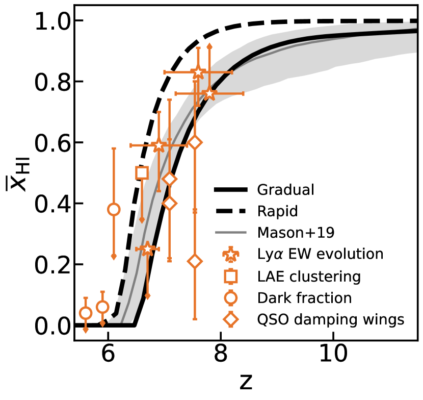
Figure 2: Example reionisation timelines for the Gradual model (solid line) and the Rapid model (dashed line) for demonstration purposes. Different symbols are neutral fractions constrained by Ly$\alpha$ equivalent width (stars, Mason et al., 2018a; Mason et al., 2019a; Bolan et al., 2022), Ly$\alpha$ emitter clustering (squares Sobacchi & Mesinger, 2015), Ly$\alpha$ forest dark pixels fraction (circles, McGreer et al., 2015), and QSO damping wings (diamonds, Davies et al., 2018a; Greig et al., 2019) observations. The grey line with shaded region is the reionisation timeline and its 16-84 percentile inferred using the aforementioned observations (Mason et al., 2019a). In the following we will use this grey posterior for $\overline{x}_{\textsc{hi}}$ for comparing to observations as a function of redshift, the Rapid and Gradual models are shown just to illustrate how these models differ when the ionisation efficiency is fixed (see Section 2.1).

2.2 Galaxy population model

To populate halos with realistic galaxy properties we use a conditional UV luminosity to halo mass relation, to assign UV luminosities, with intrinsic scatter, to our halo catalogue. We follow Ren et al. (2019) and assume UV magnitudes at a given halo mass are drawn from a Gaussian distribution with dispersion $\sigma$ and median $M_{\textsc{uv},c}(M_{\text{h}},\sigma,z)$:

$$p(M_{\textsc{uv}}\mid M_{\text{h}})=\frac{1}{\sqrt{2\pi}\sigma}\exp\left(\frac{-[M_{\textsc{uv}}-M_{\textsc{uv},c}(M_{\text{h}},\sigma,z)]^{2}}{2\sigma^{2}}\right).$$ (3)

The dispersion was originally introduced to explain scatter in the Tully–Fisher relation (Yang et al., 2005). It is a free parameter in our model, and following Whitler et al. (2020) we assume $\sigma=0.5$ mag. Ren et al. (2019) found that this value is consistent with observed luminosity functions over $z\sim 6-10$, and this value is also consistent with the expected variance due to halo assembly times (Ren et al., 2018; Mason et al., 2023). Whitler et al. (2020) found that this scatter has only a minor impact on the transmission of Ly$\alpha$ from galaxies in the reionising IGM, so we do not expect it to significantly change the relationship between galaxy luminosity and the size of the ionised bubbles they reside in.

The median relation $M_{\textsc{uv},c}(M_{\text{h}},\sigma,z)$ is set by calibration to the UV luminosity function. Ren et al. (2019) showed that above $M_{h}\,\hbox to0.0pt{\lower 3.5pt\hbox{$\mathchar 0\relax\sim$}\hss}\raise 1.0pt\hbox{$>$}\,10^{12}{M_{\odot}}$ a flattening is required in $M_{\textsc{uv},c}(M_{\text{h}})$ to maintain consistency with the observed UV LFs – which can be thought of as a critical mass or luminosity threshold for star formation. Given that our halo catalogue contains only a small number (0.001$\%$ of the total catalogue) of $>10^{12}{M_{\odot}}$ halos at $z\sim 7$, and far fewer at $z>7$ due to the steepness of the halo mass function, we do not consider this flattening. We thus use the $M_{\textsc{uv},c}(M_{\text{h}},z)$ relations from the Mason et al. (2015) UV luminosity function model as the median UV magnitudes for Equation 3. Our resulting luminosity functions are consistent with $z\sim 7-10$ observations over the range where observations are currently magnitude complete: $-22\,\hbox to0.0pt{\lower 3.5pt\hbox{$\mathchar 0\relax\sim$}\hss}\raise 1.0pt\hbox{$<$}\,{M_{\textsc{uv}}}\,\hbox to0.0pt{\lower 3.5pt\hbox{$\mathchar 0\relax\sim$}\hss}\raise 1.0pt\hbox{$<$}\,-17$ (e.g., Bouwens et al., 2021, see Appendix A).

2.3 Measuring bubble sizes

We measure the size of ionised regions, $R_{\mathrm{ion}}$ , using both the mean-free-path (MFP) method (Mesinger & Furlanetto, 2007) and the watershed algorithm (Vincent & Soille, 1991), an image segmentation algorithm which was first applied to reionisation simulations by Lin et al. (2016).

Lin et al. (2016) tested a range of approaches for estimating the sizes of ionised bubbles in simulations and determined these two methods were optimal compared to other techniques in the literature because they most accurately recover input ionised bubble size distributions, can account for overlapping bubbles, and produce sizes corresponding to a physically intuitive quantity. Other commonly used approaches for modelling the bubble size distribution, i.e. the excursion set formulation (Furlanetto et al., 2004b; Furlanetto & Oh, 2005) or approaches which grow cosmological Stromgren spheres around halos (e.g., Yajima et al., 2018) will underestimate the largest bubble sizes because these approaches do not include the effect of overlapping bubbles.

Here we describe these two methods, and their advantages and limitations. We will discuss how our resulting bubble size distributions compare to works using other methods in Section 4.1.

2.3.1 Mean free path (MFP)

This method was first used to measure ionised bubble sizes by Mesinger & Furlanetto (2007). It is essentially a Monte-Carlo ray-tracing algorithm, which enables us to measure a probability distribution for ionised bubble sizes by estimating the distance photons travel before they encounter neutral gas. We randomly choose a starting position (or the position of a galaxy, as described later), if the cell is fully ionised, we measure the distance from that position to where we encounter the first neutral or partially ionised cell at a random direction. Given our simulation resolution, the smallest bubble size we can measure is $\sim 1$ cMpc. If the position is neutral, we set ${R_{\mathrm{ion}}}=0$ cMpc. We measure bubble sizes over the full simulation volume by sampling the distance to neutral gas from $10^{5}$ random positions and sightlines to build bubble size distributions for our simulations.

In Section 3.1 we will show the bubble size distribution as a function of galaxy $M_{\textsc{uv}}$ , to estimate the sizes of ionised bubbles around observable galaxies. For this, we use the mean free path method as defined above, but start our measurements at the position of each galaxy in the simulation box.

We also will measure the bubble size distribution as a function of galaxy overdensity to compare with current observations. Galaxy overdensity depends on the dark matter density of the underlying field (e.g. Cole & Kaiser, 1989; Mo et al., 1997; Sheth et al., 2001): $n=\overline{n}(1+b\delta)$, where $n$ is the number density of galaxies observed in a field, $\overline{n}$ is the mean cosmic number density, $b$ is the bias, and $\delta$ is the dark matter density in the field. Since 21cmfast populates halos and calculates $x_{\mathrm{HI}}$ based on galaxy number density via the excursion set formulation (Furlanetto et al., 2004b), we expect a strong relation between bubble size and galaxy overdensity (e.g., Mesinger & Furlanetto, 2007).

We define the observed overdensity, $N/\langle N\rangle$ , as the number, $N$, of galaxies brighter than a given limit in a survey volume relative to the number expected in that volume based on the average in the whole simulation box, $\langle N\rangle$. To measure overdensity using our galaxy catalogue, described in Section 2.2, for a mock survey, we discard galaxies with ${M_{\textsc{uv}}}>M_{\rm UV,lim}$, where $M_{\rm UV,lim}$ is the UV magnitude limit in an observed overdensity. While the galaxy catalogue and $\overline{x}_{\textsc{hi}}$ boxes are generated from the same density field, as described in Section 2.1, galaxies are given sub-grid positions, thus to compare the overdensity and $\overline{x}_{\textsc{hi}}$ fields we convert the resulting galaxy catalogue into a galaxy number count grid of the same size as the $\overline{x}_{\textsc{hi}}$ grids. Then we convolve the galaxy number count grid with a 3-D kernel of the survey volume and divide the value of each cell by $\langle N\rangle$, the mean number count per cMpc³ in the halo box, to obtain the overdensity in each cell.

Cells in the resulting overdensity box correspond to positions with a given overdensity above the magnitude limit within the volume. We can then carry out an analogous procedure to that described above using the mean free path algorithm to find the bubble size distribution as a function of overdensity using the mean free path method, by starting in positions of a given overdensity.

2.3.2 Watershed algorithm

This method was first used to measure ionised bubble sizes in reionisation simulations by Lin et al. (2016). It is an image segmentation algorithm which treats constant values of a scalar field as contour lines corresponding to depth in a tomographic map, which it then “floods” to break up the images into separate water basins (Vincent & Soille, 1991).

We use the implementation of the watershed algorithm in skikit-image (van der Walt et al., 2014). We apply the algorithm to 3D binary $\overline{x}_{\textsc{hi}}$ cubes. We first apply the ‘distance transform’ to calculate the Euclidean distance, $d_{i}$ of every point to the nearest neutral region (if the point is neutral then the distance is zero). We invert the distances to ‘depths’: $d_{i}\rightarrow-d_{i}$. Centres of bubbles are then local minima in the depth cube and the bubble boundaries are identified by flooding regions starting from the local minima, and marking where regions meet – these are contours of constant depth $d_{i}$.

As with any image segmentation algorithm, the identification of local minima will lead to over-segmentation, as every local minimum will be marked as a unique bubble, even if it is overlapping with a larger one, thus a threshold must be used to avoid this. We follow the prescription of Lin et al. (2016) and use the ‘H-minima transform’ to essentially ‘fill in’ small basins. We identify basins with a relative depth of $h$ from the local minimum to the bubble boundary and set $d_{i}\rightarrow d_{i}+h$ for these regions, reducing the depth of the local minima. After the H-minima transform, we can again identify bubbles as above and see that large bubbles are correctly identified. This process may remove small isolated bubbles which had depth $<h$. These can be added back in manually using the initial segmentation cube.

The H-minima threshold $h$ is a free parameter, we use $h=2.5$, which is fixed so that the resulting bubble size distribution is comparable to that obtained with the MFP method above and bubbles do not suffer too much from over-segmentation. We solve for the value of $h$ by minimising the Kullback-Leibler divergence (KL divergence; Kullback, 1968) between the watershed bubble size distribution and MFP bubble distribution in a (500 cMpc)³ sub-volume of our simulation. We obtain a cube with the cells corresponding to unique bubbles labelled. From this we can calculate the volume of each bubble and calculate the size as the radius of each bubble assuming they are spherical: $R=(3V/4\pi)^{1/3}$

The watershed algorithm is a more computationally intensive method than the MFP method, and requires some tuning of the $h$ threshold, so we predominantly use the MFP approach. However, the watershed algorithm has a significant advantage in that it can measure the absolute number of bubbles in a volume. It is also possible to use it to directly connect galaxies and their host bubbles. We will use it in Section 3.5 to make forecasts for the number of large bubbles expected in upcoming wide-area surveys.

3 Results

Previous works have focused on simulating the global bubble size distribution, in order to produce predictions for 21-cm experiments (e.g. Furlanetto & Oh, 2005; Mesinger & Furlanetto, 2007; Geil et al., 2016; Lin et al., 2016). Some 21cm-galaxy cross correlation studies (e.g. Lidz et al., 2009; Park et al., 2014) calculate the correlation scales for various halo masses but do not directly calculate the bubble size distribution. Here we focus on the expected bubble size distribution around observable galaxies, which are likely to be more biased density tracers, and thus we expect are likely to trace the largest bubbles.

In Section 3.1 we present the bubble size distribution as a function of galaxy UV luminosity, and in Section 3.2 we show the bubble size distribution as a function of galaxy overdensity. The impact of different reionising source models on the bubble size distribution is discussed in Section 3.3. We demonstrate in Appendix B that our results do not significantly depend on redshift. In Section 3.4 we use our simulations to interpret recent observations of Ly$\alpha$ emission in overdensities at $z\,\hbox to0.0pt{\lower 3.5pt\hbox{$\mathchar 0\relax\sim$}\hss}\raise 1.0pt\hbox{$>$}\,7$, and we make predictions for upcoming wide-area observations in Section 3.5.

3.1 Bubble size distribution as a function of UV luminosity

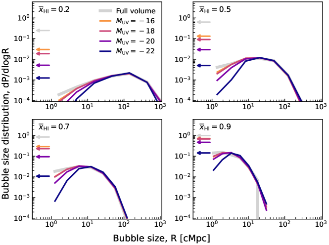
Figure 3: Bubble size distributions as a function of UV luminosity for ${M_{\textsc{uv}}}=-16,-18,-20,-22$. We also show the bubble size distribution from the full volume as a thick grey line in each simulation. The fractions of galaxies in $R<0.8$ cMpc bubbles (below our resolution limit) or neutral cells are marked with arrows. Each panel shows a different volume-averaged IGM neutral fraction, $\overline{x}_{\textsc{hi}}$ . As the neutral fraction decreases, the bubble size distributions shift to higher values, as expected as bubbles grow as reionisation progresses. With increasing UV luminosity, the probability that a galaxy resides in big bubbles increases.

To first order, UV luminosity traces dark matter halo mass and thus density (e.g., Cooray & Milosavljevic, 2005; Tempel et al., 2009; Mason et al., 2015). We thus expect the brightest galaxies to reside in the most massive halos in overdense regions, and therefore these galaxies are likely to sit in large bubbles which reionised early.

We quantify this in Figure 3, where we show the size distribution of ionised bubbles around galaxies of a given UV luminosity as a function of the volume-averaged IGM neutral fraction, $\overline{x}_{\textsc{hi}}$ , in our simulations, compared to the bubble size distribution in the full volume. This is essentially the distribution at the mean density, $\delta=0$. We measure the distribution of bubble sizes in 4 $M_{\textsc{uv}}$ bins: ${M_{\textsc{uv}}}=-16,-18,-20,-22$, with $\Delta{M_{\textsc{uv}}}=0.1$. We show our fiducial Gradual simulation but will compare it to the Rapid simulation in Section 3.3.

In contrast to previous literature we also include the fraction of galaxies (or randomly selected pixels for our full volume bubble size distribution) which are in neutral regions in our simulation. We mark these fractions with arrows in Figure 3. These sources may reside in ionised bubbles below our resolution limit ($\sim 1$ cMpc for bubble radius). Including these occurrences in our bubble size distribution leads to important insights about the environments of galaxies as we discuss below. We note that the ‘full volume’ bubble size distribution excluding neutral cells and those below our resolution limit is equivalent to the bubble size distributions presented in previous literature (e.g., Furlanetto & Oh, 2005; Mesinger & Furlanetto, 2007).

Figure 3 shows that as $\overline{x}_{\textsc{hi}}$ decreases, the bubble size distributions shift to higher values, which is expected as ionised regions grow. Compared to the bubble size distribution in the full volume, we see three important features of the bubble size distributions which we describe below.

First, while the bubble size distribution in the full volume has a high fraction of bubbles with $R\lesssim 1$ cMpc, observable galaxies (${M_{\textsc{uv}}}\lesssim-16$) are $>10-1000\times$ more likely to be in bubbles rather than neutral regions. This is because galaxies are biased tracers of the density field and therefore trace ionised regions more closely. At the end stages of reionisation, ${\overline{x}_{\textsc{hi}}}\,\hbox to0.0pt{\lower 3.5pt\hbox{$\mathchar 0\relax\sim$}\hss}\raise 1.0pt\hbox{$<$}\,0.5$, we find only $\,\hbox to0.0pt{\lower 3.5pt\hbox{$\mathchar 0\relax\sim$}\hss}\raise 1.0pt\hbox{$<$}\,10\%$ of observable galaxies are in small ionised or neutral regions below our resolution limit. This is consistent with the idea of the ‘post-overlap’ phase of reionisation (e.g., Miralda-Escudé et al., 2000), where the majority of galaxies lie within ionised regions and only voids remain to be ionised.

We see a strong trend with UV luminosity, where the brightest galaxies are always least likely to be in small ionised or neutral regions, while UV-faint galaxies have a more bimodal bubble size distribution. The proportion of UV-faint galaxies in small ionised or neutral regions is high early in reionisation: but declines rapidly from $\sim 60\%$ at ${\overline{x}_{\textsc{hi}}}\sim 0.9$ to $\sim 10\%$ at ${\overline{x}_{\textsc{hi}}}\sim 0.5$ for ${M_{\textsc{uv}}}\,\hbox to0.0pt{\lower 3.5pt\hbox{$\mathchar 0\relax\sim$}\hss}\raise 1.0pt\hbox{$>$}\,-18$ galaxies. This is driven by the clustering properties of the UV-faint galaxies as we discuss below. This may explain the low detection rate of Ly$\alpha$ in UV-faint galaxies at $z\,\hbox to0.0pt{\lower 3.5pt\hbox{$\mathchar 0\relax\sim$}\hss}\raise 1.0pt\hbox{$>$}\,8$ (Hoag et al., 2019; Mason et al., 2019a; Morishita et al., 2022) compared to the higher detection rate in UV bright galaxies seen by Jung et al. (2022) at the same redshift.

Second, we see that the bubble size distribution around observable galaxies peaks at a similar size for all $M_{\textsc{uv}}$ bins, which indicates that, on average, these galaxies are in the same bubbles. This peak, corresponding to the mean size of ionised regions, has been described as a ‘characteristic’ scale, $R_{\mathrm{char}}$ (e.g., Furlanetto & Oh, 2005). In the following we refer to the mean size of ionised regions as the characteristic size. We see that the characteristic scale of ionised regions increases by over two orders of magnitude during reionisation. However, we do find an increasing characteristic scale as a function of UV luminosity: galaxies brighter than ${M_{\textsc{uv}}}\,\hbox to0.0pt{\lower 3.5pt\hbox{$\mathchar 0\relax\sim$}\hss}\raise 1.0pt\hbox{$<$}\,-20$ are expected to reside in bubbles $\sim 1.5-2\times$ larger than the characteristic bubble scale in the full volume.

Finally, we see that the width of the bubble size distribution decreases as galaxy UV luminosity increases. This is due to the clustering of galaxies: UV bright galaxies are more likely to be in overdense regions which will reionise early, whereas UV faint galaxies can be both ‘satellites’ in overdense, large ionised regions, or ‘field galaxies’ in less dense regions which remain neutral for longer (see also Hutter et al., 2017, 2021; Qin et al., 2022) This figure demonstrates that UV-faint galaxies will have very significant sightline variance in their Ly$\alpha$ optical depth, and highlights the importance of using realistic bubble size distributions for inference of the IGM neutral fraction (see also, e.g. Mesinger & Furlanetto, 2008a; Mason et al., 2018b).

3.2 Bubble size distribution as a function of galaxy overdensity

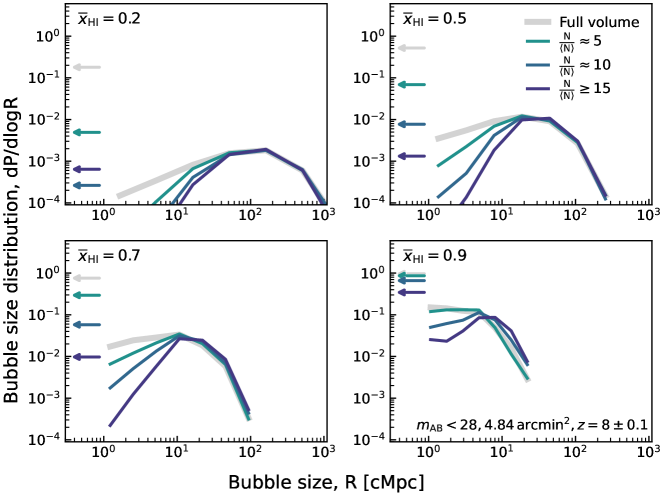
Figure 4: Bubble size distributions as a function of galaxy overdensity at $z=8\pm 0.1$ in a 4.84 arcmin² area ($\sim\left(13\mathrm{cMpc}\right)^{3}$) with a survey limit of $m_{\mathrm{A}B}=28$, for ${N/\langle N\rangle}\approx 5,10$ and $\geq 15$, where $\langle N\rangle=0.84$. We also show the bubble size distribution from the full volume as a thick grey line in each simulation. The fractions of galaxies in $R<0.8$ cMpc bubbles (below our resolution limit) or neutral cells are marked with arrows. Each panel shows a different $\overline{x}_{\textsc{hi}}$ . More overdense regions host larger $R_{\mathrm{ion}}$ early at high $\overline{x}_{\textsc{hi}}$ . As $\overline{x}_{\textsc{hi}}$ decreases, $R_{\mathrm{ion}}$ of less overdense regions begins to catch up and ends up having similar bubble size distribution to those of the most overdense regions. This agrees with the general reionisation picture, that overdense regions are reionised first.

In this section, we investigate the distribution of bubble sizes as a function of galaxy overdensity, $N/\langle N\rangle$ . This distribution should directly reflect how structure formation affects reionisation.

As described in Section 2.3 an observed galaxy overdensity, $N/\langle N\rangle$ , depends on the survey depth and volume. For our investigation here we explore expected overdensities within a medium-deep JWST observation within 1 NIRISS pointing (or $1/2$ of the NIRCam field-of-view), aiming to simulate observations similar to those obtained by the JWST/NIRISS pure-parallel PASSAGE survey (Malkan et al., 2021). We thus use a survey limiting depth of $m_{\mathrm{AB}}=28$ and area 4.84 sq. arcmin with a redshift window of $\Delta z=0.2$. This corresponds to [${M_{\textsc{uv}}}_{\mathrm{,lim}}$, $V_{\mathrm{survey}}$]=[-19, 2014 cMpc³] at $z=8\pm 0.1$. We follow the procedure described in Section 2.3 to create a cube of $N/\langle N\rangle$ using these survey parameters, and then select 200,000 cells to measure the bubble size distribution as a function of overdensity.

Figure 4 shows the bubble size distributions for ${N/\langle N\rangle}\approx 5$, ${N/\langle N\rangle}\approx 10$, and ${N/\langle N\rangle}\gtrsim 15$, along with the bubble size distribution in the full volume as a function of $\overline{x}_{\textsc{hi}}$ , for the Gradual model. As in Section 3.1 we see the clear trend that the bubble size distributions increase to higher values as the universe reionises, but we can now identify where the reionisation process begins. We can see that the most overdense regions reionise first and inhabit the largest ionised bubbles. As in Section 3.1, we investigate three clear trends in the bubble size distribution as a function of galaxy overdensity.

First, overdense regions start and finish carving out ionised bubbles earlier compared to regions at the mean density. We see a much larger proportion of overdense regions already in ${R_{\mathrm{ion}}}>1$ cMpc bubbles early in reionisation. We find at ${\overline{x}_{\textsc{hi}}}=0.9$, when only 10% of the total IGM volume is ionised, $\,\hbox to0.0pt{\lower 3.5pt\hbox{$\mathchar 0\relax\sim$}\hss}\raise 1.0pt\hbox{$>$}\,30\%$ of the ${N/\langle N\rangle}\geq 10$ regions are already in ${R_{\mathrm{ion}}}>1$ cMpc bubbles. By ${\overline{x}_{\textsc{hi}}}=0.5$, all of the ${N/\langle N\rangle}\geq 10$ regions are in ${R_{\mathrm{ion}}}>1$ cMpc bubble. This demonstrates that early in reionisation, we expect only the strongest overdensities to trace large ionised regions.

Second, ionised bubbles around overdense regions are larger than the characteristic bubble size in the full volume, particularly in the early stages of reionisation. At ${\overline{x}_{\textsc{hi}}}=0.8$, the characteristic bubble size around ${N/\langle N\rangle}\geq 10$ regions is ${R_{\mathrm{ion}}}\sim 10$ cMpc, which is $\sim 2\times$ larger than the mean bubble size in the full volume at that time, and large enough for significant Ly$\alpha$ transmission (e.g., Miralda-Escude, 1998; Mason & Gronke, 2020; Qin et al., 2022). Detection of Ly$\alpha$ in a highly neutral universe is thus not unexpected if the LAEs are in highly overdense regions.

The mean bubble size of overdense regions grow more slowly than that of less overdense regions. In the early stage of reionisation, bubbles around the most overdense regions grow in isolation and do not merge with similarly sized bubbles because most overdense regions are far away from each other. By contrast, bubbles created by less overdense regions are more likely to grow rapidly by merging with other bubbles.

Finally, again we see the bubble size distributions are broad, but that the strong overdensities have the narrowest distribution of bubble sizes because they are guaranteed to trace ionised environments, whereas less dense regions can be isolated, and therefore in smaller bubbles, or contained within large scale overdensities in large bubbles.

3.3 Bubble size distribution as a function of reionising source model

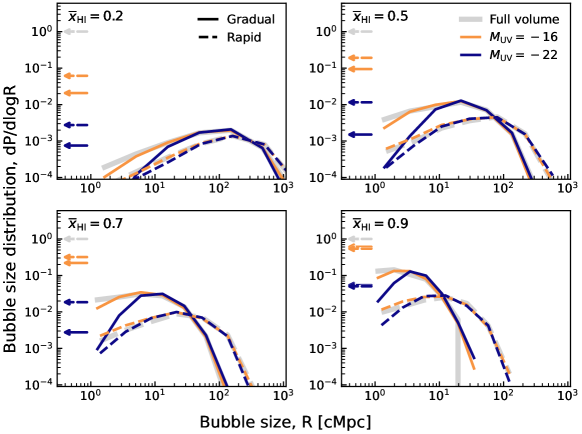
Figure 5: Bubble size distributions as a function of UV luminosity for ${M_{\textsc{uv}}}=-16,-22$, for the Gradual (solid lines) and Rapid (dashed lines) reionisation models. We also show the bubble size distribution in the full volume as a thick grey line for each simulation. The fractions of galaxies in $R<0.8$ cMpc bubbles (below our resolution limit) or neutral cells are marked with arrows. Each panel shows a different volume-averaged IGM neutral fraction. We see that the bubble size distributions are broader for the Rapid models than for the Gradual model at ${\overline{x}_{\textsc{hi}}}\,\hbox to0.0pt{\lower 3.5pt\hbox{$\mathchar 0\relax\sim$}\hss}\raise 1.0pt\hbox{$>$}\,0.5$. The bubble size distributions of the Rapid model peak at ${R_{\mathrm{ion}}}\gtrsim 10$cMpc since as early as ${\overline{x}_{\textsc{hi}}}=0.9$. By contrast the distributions of Gradual models start with ${R_{\mathrm{ion}}}\lesssim 6$ cMpc at ${\overline{x}_{\textsc{hi}}}=0.9$, and gradually evolve to converge with the Rapid models as IGM becomes more ionised.

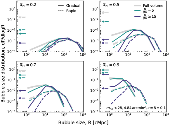
Figure 6: Bubble size distributions as a function of overdensity for ${N/\langle N\rangle}=5,>15$, for the Gradual (solid lines) and Rapid (dashed lines) reionising source models. We also show the total bubble size distribution as a thick grey line in each simulation. The fractions of galaxies in $R<0.8$ cMpc bubbles (below our resolution limit) or neutral cells are marked with arrows. Each panel shows a different volume-averaged IGM neutral fraction. In the Rapid model we see that bubble size distribution of ${N/\langle N\rangle}>7$ already shows little bimodality at ${\overline{x}_{\textsc{hi}}}=0.9$. Galaxies in ${N/\langle N\rangle}>15$ regions are mostly in bubbles of ${R_{\mathrm{ion}}}>7$. In contrast, in Gradual model even galaxies in ${N/\langle N\rangle}>5$ regions are in bubbles of ${R_{\mathrm{ion}}}<7$.

In the previous sections we have shown the bubble size distribution using only our fiducial Gradual  faint-galaxies driven, reionisation model. Here we demonstrate how the bubble size distribution changes if instead reionisation is driven by rarer, brighter galaxies in our Rapid model. We show the bubble size distributions for the two models as a function of the IGM neutral fraction in Figures 5 and  6 for galaxies of given $M_{\textsc{uv}}$ and galaxy overdensities.

Both models have qualitatively similar bubble size distributions but the Rapid model predicts much large bubble sizes at fixed neutral fraction, particularly at the earliest stages of reionisation. A key prediction of the Rapid model is the existence of large ($\sim 30-100$ cMpc) bubbles at the earliest stages of reionisation, ${\overline{x}_{\textsc{hi}}}\sim 0.9$, in order to fill the same volume with ionised hydrogen around the more biased ionising sources.

First, galaxies in the Gradual model are more likely to reside in neutral IGM at the beginning of reionisation, compared to galaxies in the Rapid model. At ${\overline{x}_{\textsc{hi}}}=0.9$, $\sim 80\%$ of the ${M_{\textsc{uv}}}=-16$ galaxies have bubble sizes no greater than $1$ cMpc in the Gradual model. By contrast, in the Rapid model, only $\sim 60\%$ of ${M_{\textsc{uv}}}=-16$ galaxies are in such neutral regions at the same $\overline{x}_{\textsc{hi}}$ . At the mid-point of reionisation (${\overline{x}_{\textsc{hi}}}=0.5$), UV-faint galaxies (${M_{\textsc{uv}}}=-16$) in the Gradual model ($\sim 9\%$) are half as likely to be in small ionised/neutral regions compared to UV-faint galaxies in the Rapid model ($\sim 20\%$). This is because the early ionised regions in the Rapid model are concentrated around the most overdense regions, compared to a more uniform coverage of bubbles seen in the Gradual model (see Figure 1). In the Rapid model isolated faint galaxies cannot create ${R_{\mathrm{ion}}}>1$ cMpc bubbles around themselves, because reionisation is dominated by ${M_{\textsc{uv}}}\,\hbox to0.0pt{\lower 3.5pt\hbox{$\mathchar 0\relax\sim$}\hss}\raise 1.0pt\hbox{$<$}\,19.5$ galaxies in this model. Therefore isolated faint galaxies remain in ${R_{\mathrm{ion}}}<1$ cMpc bubbles even at the mid-point of the reionisation.

Second, galaxies in the Rapid model blow out big ionised bubbles early in the reionisation. However, the bubble sizes do not grow as rapidly as those in the Gradual model. At the beginning of reionisation, the characteristic bubble size in the Rapid model is ${R_{\mathrm{char}}}\approx 10$ cMpc. In the Gradual model, the characteristic bubble size $\sim 3\times$ smaller: no more than 3 cMpc. By the late stages of reionisation (${\overline{x}_{\textsc{hi}}}=0.1$), the mean bubble sizes in the Rapid model are $\sim 300$ cMpc. However, in the Gradual model, the mean bubble size has grown twice as rapidly, reaching $\sim 200$ cMpc. The different evolutionary trends reflect the different bubble-merging histories of the two models. In the Gradual scenario, many faint galaxies create small ionised bubbles and soon merge together to form big bubbles. In the Rapid model, big bubbles form early, however, but due to the rarity of bright ionising galaxies, bubbles are less likely to merge and immediately double in size compared to those in the Gradual model.

We can see from this comparison that there can be a degeneracy between the Gradual and Rapid model. If we find evidence of a large ($>10$ cMpc) bubble at high redshift, it could be explained by a bright-galaxies-driven reionisation at a high neutral fraction, or by the faint-galaxies-driven reionisation but with a lower neutral fraction. However, independent information on the reionisation history and/or information from the dispersion of bubble sizes along multiple sightlines could break this degeneracy. We discuss this in Section 4.2.

3.4 Interpretation of current observations

Table 1: Assumed properties of $z\,\hbox to0.0pt{\lower 3.5pt\hbox{$\mathchar 0\relax\sim$}\hss}\raise 1.0pt\hbox{$>$}\,7$ associations of Ly$\alpha$ emitters used in our simulations.

							$p(R>1\,\mathrm{pMpc})^{\ast}$
Field	$z$	$N_{\mathrm{LAEs}}$	Minimum $M_{\textsc{uv}}$	$\overline{x}_{\textsc{hi}}$ †	Volume‡ [pMpc3]	Overdensity	Full volume	In overdensity	$R_{\mathrm{char}}$ ∗ [pMpc]	References
COSMOS	6.8	9	$-20.4$	$0.44^{+0.09}_{-0.17}$	140	$>3$	0.52 (0.72)	0.93 (0.99)	6.4 (11.2)	[1]
BDF	7.0	3	$-19.5$	$0.56^{+0.09}_{-0.08}$	53	$>3$	0.27 (0.57)	0.84 (0.98)	3.1 (6.3)	[2-5]
EGS	7.7	7	$-19.5$	$0.76^{+0.05}_{-0.09}$	2.6	$>3$	0.07 (0.26)	0.39 (0.67)	1.0 (2.2)	[6-10]
Abell 2744	7.9	0	$-17.7$	$0.80^{+0.06}_{-0.09}$	0.001	$>130$	0.10 (0.29)	0.27 (0.53)	0.5 (1.6)	[11,12]
EGS	8.7	2	$-19.5$	$0.93^{+0.02}_{-0.15}$	12	$>3$	0.01 (0.07)	0.11 (0.42)	0.8 (1.6)	[8,9,13,14]
GOODS-N	10.6	1	$-18.6$	$>0.92$	2.6	$>24$	0.004 (0.02)	0.07 (0.48)	0.5 (1.1)	[15-17]

^† Using the non-parametric reionisation history posteriors by Mason et al. (2019a) including constraints from the CMB optical depth, quasar dark pixel fraction and measurements of the Ly$\alpha$ damping wing in quasars and galaxies. We calculate $p(R>1\,\mathrm{pMpc})$ by marginalising $p(R>1\,\mathrm{pMpc}|{\overline{x}_{\textsc{hi}}})$ over the $\overline{x}_{\textsc{hi}}$ posterior at each redshift inferred by Mason et al. (2019a). ^‡We assume a redshift window of $\Delta z=0.2$ except for the COSMOS and Abell 2744 regions which are spectroscopically confirmed. For those regions we use the volumes estimated by Endsley & Stark (2022) and Morishita et al. (2022) respectively.
^∗ Calculated using Gradual  (Rapid). [1] Endsley & Stark (2022), [2] Vanzella et al. (2011), [3] Castellano et al. (2016), [4] Castellano et al. (2018), [5] Castellano et al. (2022), [6] Oesch et al. (2015), [7] Tilvi et al. (2020), [8] Leonova et al. (2022), [9] Tang et al. (2023), [10] Jung et al. (2022), [11] Morishita et al. (2022), [12] Ishigaki et al. (2016), [13] Zitrin et al. (2015b), [14] Larson et al. (2022), [15] Oesch et al. (2016), [16] Bunker et al. (2023), [17] Tacchella et al. (2023).

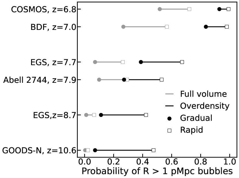
Figure 7: Probability in our models of finding a bubble size $>1$ pMpc around regions similarly overdense to the observed $z\,\hbox to0.0pt{\lower 3.5pt\hbox{$\mathchar 0\relax\sim$}\hss}\raise 1.0pt\hbox{$>$}\,7$ associations of Ly$\alpha$ emitters in our Gradual and Rapid simulations (black lines). Grey lines show the range of probabilities in the full simulation volume. We use the IGM neutral fractions expected at these redshifts (Mason et al., 2019b). The plot is discussed in Section 3.4 and a summary of our simulation setup is given in Table 1. The bubble size distributions for all these fields is shown in Figure 13. It is highly likely for the observed $z\sim 7$ Ly$\alpha$ emitting galaxies to reside in large ionised bubbles. At $z\gtrsim 8$, large bubbles are unexpected even in overdensities.

In this section, we use our simulations to interpret some recent observations of Ly$\alpha$ emission at $z\,\hbox to0.0pt{\lower 3.5pt\hbox{$\mathchar 0\relax\sim$}\hss}\raise 1.0pt\hbox{$>$}\,7$ in candidate overdensities. Here we aim to establish if the enhanced Ly$\alpha$ visibility in these regions can be explained by the sources tracing an ionised overdensity, and how likely that scenario is given our consensus timeline of reionisation and either of our two reionisation models.

We focus on observations of $z\,\hbox to0.0pt{\lower 3.5pt\hbox{$\mathchar 0\relax\sim$}\hss}\raise 1.0pt\hbox{$>$}\,7$ Ly$\alpha$ emission from galaxies in 6 regions in the sky, in candidate overdensities: the COSMOS field at $z\approx 6.8$ (Endsley & Stark, 2022), BDF field at $z\approx 7.0$ (Vanzella et al., 2011; Castellano et al., 2016, 2018, 2022), EGS field with two regions at $z\approx 7.7$ and 8.7 (Oesch et al., 2015; Roberts-Borsani et al., 2016; Tilvi et al., 2020; Leonova et al., 2022; Larson et al., 2022; Jung et al., 2022; Tang et al., 2023), the field behind the galaxy cluster Abell 2744 at $z\approx 7.9$ (Morishita et al., 2022) and the area around the $z=10.6$ galaxy GNz11 (Oesch et al., 2016; Bunker et al., 2023; Tacchella et al., 2023).

To compare with observations at known redshifts, we will switch from comoving to proper distance units. Due to the incompleteness of the observations, here we aim to create bubble size distributions for regions in our simulations that are approximately similar to those observed. Our simulations are coeval boxes at $z=7,8,9,10$, so in the following we use the box closest in redshift to the observations, but use the observed redshift to fix assumed IGM neutral fractions and to calculate physical distances. We demonstrate in Appendix B that our bubble size distributions do not depend significantly on redshift.

We create mock observations assuming the same area as the observed overdensities. For the regions which only have photometric overdensities, due to the large redshift uncertainties in the photometric overdensities, but motivated by the $\Delta z\,\hbox to0.0pt{\lower 3.5pt\hbox{$\mathchar 0\relax\sim$}\hss}\raise 1.0pt\hbox{$<$}\,0.2$ redshift separation of Ly$\alpha$ emitters in all of these regions, we assume a redshift window of $\Delta z=0.2$ for our mock observations. This corresponds to $\sim 5-8$ pMpc at $z\sim 7-10$. In all cases we will assume the observed overdensity of Lyman-break galaxies to be the same in that smaller volume as in the true observed volume. This means we are likely overestimating the true overdensity, in that case our estimated probabilities can be seen as upper limits.

Using these assumed volumes we then use the method described in Section 2.3.1 to convolve our galaxy field with the volume and depth kernel of the observations to create a cube of overdensity matched to each observation setup. We then select regions in the overdensity cube which match the observed overdensity estimates.

We assess the probability of the observed overdensities lying in ionised regions $>1$ pMpc in radius, which would allow $\,\hbox to0.0pt{\lower 3.5pt\hbox{$\mathchar 0\relax\sim$}\hss}\raise 1.0pt\hbox{$>$}\,30\%$ of Ly$\alpha$ flux to be transmitted at the rest frame Ly$\alpha$ line centre (up to $\sim 50\%$ transmission for emission 500 km s^-1 redward of linecentre, e.g., Mason & Gronke, 2020; Qin et al., 2022). While the true Ly$\alpha$ detection rate will depend on the flux limit of the survey and the Ly$\alpha$ flux emitted by the galaxies, before attenuation in the IGM, this threshold gives us a qualitative approach with which to interpret the observations. We defer full forward-modelling of Ly$\alpha$  observations to a future work. At the redshift of each observation we assume a non-parametric estimate of the IGM neutral fraction, $\overline{x}_{\textsc{hi}}$ , inferred by Mason et al. (2019b) described in Section 2.1. We then calculate the final bubble size distribution by marginalising the bubble size distribution at each $\overline{x}_{\textsc{hi}}$ over the inferred $\overline{x}_{\textsc{hi}}$ distribution. We also measure the characteristic bubble sizes, ${R_{\mathrm{char}}}$, for the observed overdensities, which indicates the mean size of ionised regions above our resolution limit around the overdensities.

We present a summary of our simulation setups to compare to these observations in Table 1, the resulting probability of each region residing in a large ionised region in Figure 7, and $R_{\mathrm{char}}$ . The full bubble size distributions are described in Appendix C.

3.4.1 $z\sim 7$ overdensities in COSMOS and BDF fields

In the COSMOS field, Endsley & Stark (2022) detected Ly$\alpha$ in 9/10 ${M_{\textsc{uv}}}\lesssim-20.4$, $z\approx 6.8$ galaxies in a 140 pMpc³ volume. Using these spectroscopic confirmations, they estimate the lower limit of the overdensity of this region is $\gtrsim 3$. They estimate that individual galaxies in this field can create ionised bubbles ${R_{\mathrm{ion}}}\sim 0.69-1.13$ pMpc. Taking into account the ${N/\langle N\rangle}\sim 3$ overdensity and the ionising contribution from ${M_{\textsc{uv}}}<-17$ galaxies, they estimate an ionised bubble radius of ${R_{\mathrm{ion}}}\sim 3$ pMpc in this volume.

We predict that almost 100% of regions this overdense at ${\overline{x}_{\textsc{hi}}}\approx 0.5$ are in $>1$ pMpc bubbles and the characteristic bubble size is ${R_{\mathrm{char}}}=6.4$ pMpc at ${\overline{x}_{\textsc{hi}}}\approx 0.4$. The high LAE fraction detected by Endsley & Stark (2022) is thus consistent with being a typical ionised region in our Gradual model. In the Rapid model, we predict even larger bubble sizes around this overdensity: the characteristic bubble size is ${R_{\mathrm{char}}}=11.2$ pMpc, thus high Ly$\alpha$ transmission would also be expected. In both cases we would expect an excess of Ly$\alpha$ detections in neighbouring UV-faint galaxies.

In the BDF field, Vanzella et al. (2011) and Castellano et al. (2018) detected 3 $z\sim 7.0$ LAEs, with ${M_{\textsc{uv}}}=[-21.1,-20.4,-20.4]$. Two of the galaxies have a projected separation of only 91.3 pkpc, and the third is 1.9 pMpc away (Castellano et al., 2018). The photometric overdensity of $z\sim 7$ Lyman-break galaxies within $\sim 3.86$ arcmin² around these galaxies is $3-4\times$ times higher than expected (Castellano et al., 2016). Based on the star formation rate and age of the galaxies, and assuming a uniform IGM ${\overline{x}_{\textsc{hi}}}=0.5$ surrounding the sources, Castellano et al. (2018) estimated individual bubble sizes of the two galaxies at $\sim 2$ pMpc separation to be ${R_{\mathrm{ion}}}<0.8$ pMpc. We use a 56 arcmin² survey area (corresponding to the BDF field, where the sources have an angular separation of 6 arcmin, Vanzella et al., 2011) at $z=7\pm 0.1$, which is $>3\times$ overdense (Castellano et al., 2016). We see in Figure 7 that we expect nearly all regions ($\sim 84\%$ in our fiducial Gradual model) with this galaxy overdensity to be inside $>1$ pMpc ionised bubbles, enabling significant Ly$\alpha$ escape.

The non-detection of Ly$\alpha$ with equivalent width $>25$ Å in twelve surrounding UV-faint galaxies in this region may thus be surprising, but could be explained by a number of reasons, as discussed by Castellano et al. (2018). For example, even given the predicted most likely bubble size of 4 pMpc the fraction of transmitted Ly$\alpha$ flux may be only $\sim 60\%$ for galaxies at the centre of the bubble (Mason & Gronke, 2020), thus with deeper spectroscopy Ly$\alpha$ may be detected. It could also be possible that infalling neutral gas in this region resonantly scatters Ly$\alpha$ photons emitted redward of systemic (which look blue in the rest-frame of the infalling gas, e.g., Santos, 2004; Weinberger et al., 2018; Park et al., 2021). As UV-faint galaxies are likely to be low mass, and thus have a lower HI column density in the ISM compared to UV-bright galaxies, they may emit more of their Ly$\alpha$ close to systemic redshift, making it more easily susceptible to scattering by infalling gas. Measurements of systemic redshifts for the galaxies in this region may help explain the complex Ly$\alpha$ visibility. Furthermore, given the large photometric redshift uncertainties of the Castellano et al. (2016) sample, it could also be possible that the actual galaxy overdensity associated with the three LAEs is smaller, thus the expected bubble size is smaller and the faint galaxies may not lie in the same bubble as the detected LAEs.

3.4.2 $z\sim 8$ overdensities in EGS and Abell 2744 fields

The EGS field contains the majority of $z>7$ LAEs that have been detected to-date (Zitrin et al., 2015a; Oesch et al., 2015; Roberts-Borsani et al., 2016; Tilvi et al., 2020; Larson et al., 2022; Jung et al., 2022; Tang et al., 2023). Among these LAEs, Tilvi et al. (2020), Jung et al. (2022) and Tang et al. (2023) have reported a total of 8 ${M_{\textsc{uv}}}<-20$ $z\approx 7.7$ LAEs, including the ${M_{\textsc{uv}}}=-22$ LAE detected by Oesch et al. (2015), within a circle of radius $\approx 1$ pMpc. Jung et al. (2022) estimates the ${R_{\mathrm{ion}}}<1.1$ pMpc for the individual galaxies based on the model of Yajima et al. (2018) which relates Ly$\alpha$ luminosity and bubble size. The photometric overdensity around these LAEs has been estimated to be ${N/\langle N\rangle}\sim 3-5$ (Leonova et al., 2022).

We calculate the bubble size distributions using a setup similar to the results of Leonova et al. (2022): an area of 4.5 arcmin² at $z=7.7\pm 0.1$, with a limiting UV magnitude ${M_{\textsc{uv}}}>-19.5$. The result is shown in Figure 7, assuming the neutral fraction ${\overline{x}_{\textsc{hi}}}(z=7.7)=0.76_{-0.09}^{+0.05}$ (Mason et al., 2019b). We find $\sim 40\%$ of regions this overdense are in large ionised bubbles in the Gradual model and 70% of regions in the Rapid model. We conclude this region is likely consistent with our consensus picture of reionisation.

In the Abell 2744 field, Morishita et al. (2022) found no Ly$\alpha$ detections of 7 $z\approx 7.89$, ${M_{\textsc{uv}}}>-20$ galaxies. These galaxies are within a circle of radius $\sim$60 pkpc. This area is ${N/\langle N\rangle}\sim 130$ overdense for galaxies with ${M_{\textsc{uv}}}>-17.5$ (Ishigaki et al., 2016). Morishita et al. (2022) estimated bubble sizes of ${R_{\mathrm{ion}}}\sim 0.07-0.76$ pMpc for individual galaxies, based on their ionising properties derived from rest-frame optical spectroscopy with NIRSpec. We generate the bubble size distributions for a region of $>130\times$ overdensity of ${M_{\textsc{uv}}}\,\hbox to0.0pt{\lower 3.5pt\hbox{$\mathchar 0\relax\sim$}\hss}\raise 1.0pt\hbox{$<$}\,-17.5$ galaxies within a volume of (0.9 cMpc)³. A bubble size of ${R_{\mathrm{ion}}}\sim 1$pMpc or larger is unexpected for regions as overdense as this in our Gradual model at ${\overline{x}_{\textsc{hi}}}\sim 0.8$: we find $p(R>1\mathrm{pMpc})=0.27$.

The redshifts of sources in the EGS and Abell2744 fields are very similar. However, Ly$\alpha$ has only been detected in the EGS field. We can see in Figure 7 and Table 1 that our predicted bubble size distributions for EGS are shifted towards higher bubble sizes than in Abell 2744. Although the Abell 2744 region is overdense in UV-faint galaxies, the volume of this region is very small, thus there may not be sufficient ionising emissivity to produce a large-scale ionised region. Thus non-detection of Ly$\alpha$ in this overdensity is not surprising.

3.4.3 $z\sim 9-11$ overdensities in EGS and GOODS-N fields

The highest redshift association of LAEs in the EGS field is a pair at $z\approx 8.7$ (Zitrin et al., 2015b; Larson et al., 2022), which lies $\sim 4$ pMpc apart. The photometric overdensity around these LAEs has been estimated to be ${N/\langle N\rangle}\sim 3-5$ (Leonova et al., 2022). We calculate the bubble size distributions using a setup similar to the results of Leonova et al. (2022): an area of 27 arcmin² (corresponding to $\sim 6$ HST/WFC3 pointings between the two sources) with $\Delta z=0.2$, with a limiting UV magnitude ${M_{\textsc{uv}}}>-19.5$.

At $z=8.7$ the inferred IGM neutral fraction is ${\overline{x}_{\textsc{hi}}}=0.93_{-0.15}^{+0.02}$. We predict the probability of finding LAEs at ${\overline{x}_{\textsc{hi}}}\approx 0.9$ should be extremely low: in the full simulation volume in our fiducial Gradual model, we obtain $p(R>1\mathrm{pMpc})=0.01$ and there is $<0.2$% probability of finding a bubble with ${R_{\mathrm{ion}}}>4$ pMpc. Around regions as overdense as that observed we find $p(R>1\mathrm{pMpc})=0.11$. Thus in our fiducial model, we find it is extremely unlikely that the $z\approx 8.7$ LAE pair in the EGS field are in one large ionised region.

The visibility of Ly$\alpha$  therefore implies some missing aspect in our understanding of this system. If ${\overline{x}_{\textsc{hi}}}$ is lower, there will be a higher chance to find LAEs: we obtain $p(R>1\mathrm{pMpc})=0.17$ in regions this overdense if ${\overline{x}_{\textsc{hi}}}=0.8$, so $\overline{x}_{\textsc{hi}}$ will need to be substantially lower to find a high probability of large ionised regions. Alternatively, in the Rapid model, $p(R>1\mathrm{pMpc})=0.42$ for such an overdensity, and the bubble size distributions at ${\overline{x}_{\textsc{hi}}}=0.8-0.6$ peak at ${R_{\mathrm{ion}}}\gtrsim 3$ pMpc: the two LAEs could be in one large ionised bubble. Finally, the Ly$\alpha$  visibility of these galaxies could be boosted by high intrinsic Ly$\alpha$ production as suggested by their other strong emission lines, and potential contribution of AGN (Stark et al., 2017; Tang et al., 2023; Larson et al., 2023), and facilitated transmission in the IGM if the Ly$\alpha$ flux is emitted redward of systemic (e.g., Dijkstra et al., 2011; Mason et al., 2018b).

Finally, Bunker et al. (2023) have detected Ly$\alpha$ in GN-z11 at $z=10.6$, in the GOODS-N field (Oesch et al., 2016). 9 fainter galaxy candidates ($m_{\rm AB}\approx 29$) at similar redshift are found within a (10 cMpc)² square centred at GN-z11 (Tacchella et al., 2023). We estimate the overdensity of $m_{\rm AB}<29$ (${M_{\textsc{uv}}}<-18.6$), $z=10\pm 0.1$ galaxies in this field using our $z=10$ UV LF, finding that this region is $\sim 23\times$ overdense. We obtain $p(R>1\mathrm{pMpc})=0.07$ and 0.48 in the Gradual and the Rapid model, respectively. It is thus extremely unlikely that all of the $z\sim 11$ galaxies are in one $R>1\mathrm{pMpc}$ ionised region that allows significant Ly$\alpha$ transmission, in our fiducial Gradual model.

We find ${R_{\mathrm{char}}}=0.5$ and 1.1 pMpc in the Gradual and the Rapid model, respectively. The characteristic bubble size is slightly smaller than the largest distance of galaxies from GN-z11 in this field ($\sim 0.6$ pMpc) estimated by Tacchella et al. (2023) from photometric redshifts, implying that most of these galaxies could reside in the same (small) ionised region.

In summary, our simulations demonstrate that the regions discussed above at $z\sim 7$ are extremely likely ($>90\%$) to be in large ionised bubbles, given their large estimated overdensities. We also find it likely ($\,\hbox to0.0pt{\lower 3.5pt\hbox{$\mathchar 0\relax\sim$}\hss}\raise 1.0pt\hbox{$>$}\,40\%$) that the EGS region at $z\approx 7.7$ is in a large ionised bubble. However, at higher redshifts we find it very unlikely that the $z\approx 8.7$ Ly$\alpha$ -emitters in EGS and the $z\approx 10.6$ galaxies in GOODS-N, including GNz11, are in large ionised regions ($\sim 11\%$ and $\sim 7\%$ respectively) in our fiducial Gradual model.

If the actual overdensities of these regions are smaller than the photometrically estimated values, we will find it even more unlikely for these galaxies to reside in large ionised bubbles, strengthening our result. These results clearly demonstrate the importance of measuring the IGM neutral fraction at $z\,\hbox to0.0pt{\lower 3.5pt\hbox{$\mathchar 0\relax\sim$}\hss}\raise 1.0pt\hbox{$>$}\,8$ and distinguishing between reionising source models (e.g., Bruton et al., 2023), and of understanding intrinsic Ly$\alpha$ production and escape in the ISM in these galaxies (Roberts-Borsani et al., 2022; Tang et al., 2023).

3.5 Forecasts for future observations

Anticipating upcoming large area surveys at $z\,\hbox to0.0pt{\lower 3.5pt\hbox{$\mathchar 0\relax\sim$}\hss}\raise 1.0pt\hbox{$>$}\,7$ we make forecasts for the expected number of large bubbles in the JWST COSMOS-Web survey (Casey et al., 2022), the Euclid Deep survey (Euclid Collaboration et al., 2022; van Mierlo et al., 2022), and the Roman High-Latitude Survey (Wang et al., 2022). These surveys will detect tens of thousands of UV-bright $z>7$ galaxy candidates which could be used to constrain the underlying density field and pinpoint early nodes of reionisation.

The identification of ionised regions in these large surveys has the potential to distinguish between reionisation models. We sample simulated volumes equivalent to the survey areas (0.6 sq. degrees for COSMOS-Web, 53 sq. degrees for Euclid-Deep) at $z=8\pm 0.1$ and use the watershed algorithm (Section 2.3.2) to identify individual bubbles in these volumes. As we describe below the bubble size distribution in a Euclid Deep-like survey volume will suffer minimal cosmic variance, thus our Euclid forecast can be rescaled to forecast for the the Roman High-Latitude Survey (2000 sq. deg). We show in Appendix B that the expected bubble sizes, in comoving units, do not depend strongly on redshift, so our results can be easily shifted to other redshifts without expecting significant differences. As discussed above, to reduce over-segmentation we use the H-minima threshold when calculating the bubble sizes using the watershed algorithm, this sets an effective resolution of 3 cMpc.

In Figure 8 we plot our predicted ‘bubble size function’ down to this resolution limit: the number density of ionised bubbles as a function of bubble size, for our Gradual and Rapid model at ${\overline{x}_{\textsc{hi}}}=[0.5,0.7,0.9]$. The number of bubbles with $R\,\hbox to0.0pt{\lower 3.5pt\hbox{$\mathchar 0\relax\sim$}\hss}\raise 1.0pt\hbox{$>$}\,10$ cMpc can be considered a proxy for a cluster of Ly$\alpha$ -emitting galaxies, as $\sim 30-50\%$ of Ly$\alpha$ flux should be transmitted through regions this large (Mason & Gronke, 2020). As the neutral fraction decreases, as above, we expect to find an increasing number of large ionised regions, and the number of small ionised regions decreases as bubbles overlap. Figure 8 again shows the clear difference in the predicted number and size of ionised regions for the different reionisation models, as discussed in Section 3.3. We mark the survey volume of COSMOS-Web and Euclid Deep, (120cMpc)³ and (530cMpc)³ at $z=8$, respectively, as horizontal lines. The survey volume of the Roman High-Latitude survey (not shown) is (1816cMpc)³.

We note that when ${\overline{x}_{\textsc{hi}}}\,\hbox to0.0pt{\lower 3.5pt\hbox{$\mathchar 0\relax\sim$}\hss}\raise 1.0pt\hbox{$<$}\,0.7$ we expect a significant fraction of bubbles with $R\,\hbox to0.0pt{\lower 3.5pt\hbox{$\mathchar 0\relax\sim$}\hss}\raise 1.0pt\hbox{$>$}\,50$ cMpc (see Figures 3 and 4). COSMOS-Web is thus unlikely to capture the full extent of large ionised bubbles. Kaur et al. (2020) demonstrated that a simulated volume of $>$(250 cMpc)³ is required for convergence of the 21-cm power spectrum during reionisation, so it is likely that a similar volume must be observed to be able to robustly measure the bubble size distribution, thus we expect the Euclid Deep and Roman High Latitude surveys can robustly sample the full bubble size distribution.

However, to detect $R>10$ cMpc ionised bubbles, requires not only a large survey volume, but sufficient survey depth to detect the high redshift UV-bright galaxies which signpost large ionised regions. Only the Roman Space Telescope (RST) (Akeson et al., 2019) is likely to be able to carry out bubble counting. Zackrisson et al. (2020) study the number of galaxies within a $\mathrm{V}_{\rm ion}=1000$ cMpc³ bubble that can be detected with upcoming photometric surveys with instruments such as Euclid, JWST, and RST. They found that the Euclid Deep survey can barely detect one ${M_{\textsc{uv}}}\approx-21$ galaxy in that volume at $z>7$ given its detection limit, meaning that identifying large overdensities will be challenging. By contrast, a $\approx 20$ deg² deep field observation by RST could detect $\sim 10\,{M_{\textsc{uv}}}\,\hbox to0.0pt{\lower 3.5pt\hbox{$\mathchar 0\relax\sim$}\hss}\raise 1.0pt\hbox{$<$}\,-18.5$ galaxies at $z=7-10$ in a $\mathrm{V}_{\rm ion}=1000$ cMpc³ volume. The wide survey area ($\approx$ (400 cMpc)³ at $z\sim 8\pm 0.2$) and survey depth of a RST deep field observation will allow us to identify the UV-bright galaxies which trace large ionised regions. Deeper imaging or slitless spectroscopy around the UV-bright sources, for example with JWST to confirm overdensities, followed by Ly$\alpha$ spectroscopy of these regions would enable estimates of the number density of ionised bubbles.

These results demonstrate that counting the number of overdensities of LAEs in a volume can be a useful estimate of the bubble size distribution, as they will probe ionised regions $\,\hbox to0.0pt{\lower 3.5pt\hbox{$\mathchar 0\relax\sim$}\hss}\raise 1.0pt\hbox{$>$}\,1$ pMpc, and thus $\overline{x}_{\textsc{hi}}$ (especially at ${\overline{x}_{\textsc{hi}}}>0.5$). For example, in our fiducial Gradual model we expect no $R>10$ cMpc bubbles in the COSMOS-Web volume when ${\overline{x}_{\textsc{hi}}}=0.9$. This implies detection of clusters of LAEs in this volume at a given redshift would indicate ${\overline{x}_{\textsc{hi}}}<0.9$ (or a reionisation morphology similar to our Rapid model). We expect tens of large bubbles in this volume when ${\overline{x}_{\textsc{hi}}}<0.7$. However, multiple sightline observations, for example, a counts-in-cells approach can be a more efficient tool to recover the distribution than a single area survey (e.g., Mesinger & Furlanetto, 2008b).

However, bubble size functions in a COSMOS-Web-like survey volume have high cosmic variance, making it challenging to measure $\overline{x}_{\textsc{hi}}$ precisely. In Figure 9 we plot the median number of bubbles that can be observed by a COSMOS-Web-like survey using 50 realisations along with the 16-84 percentile number counts for our Gradual model. The variance is large enough to make the bubble size functions at ${\overline{x}_{\textsc{hi}}}=0.5-0.7$ indistinguishable. We do not plot the variance for the Rapid model for clarity, but when taking that into account, we cannot discriminate between the bubble size functions of Gradual and Rapid with a COSMOS-Web-like survey.

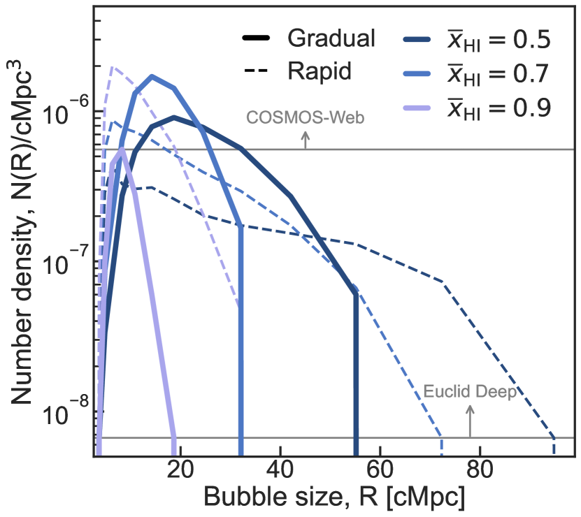
Figure 8: Number density of ionised bubbles for a range of $\overline{x}_{\textsc{hi}}$ and for our Gradual (solid) and Rapid models (dashed), calculated using the watershed algorithm. We show the inverse of the survey volume for COSMOS-Web (120 cMpc)³ and Euclid Deep (530 cMpc)³ as horizontal lines, marking the number density where one bubble is expected in that volume.

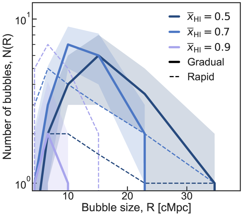
Figure 9: Number of ionised bubbles we predict from multiple realisations of a COSMOS-Web-like survey for our Gradual and Rapid models at a range of neutral fractions. The lines show the median number counts and the shaded regions are the 16-84 percentile of the number counts, demonstrating the large cosmic variance in this volume.

4 Discussion

In the following section we compare our results to those obtained from other simulations (Section 4.1) and discuss the implications of our results for the reionisation history and identifying the primary sources of reionisation (Section 4.2).

4.1 Comparison to other simulations

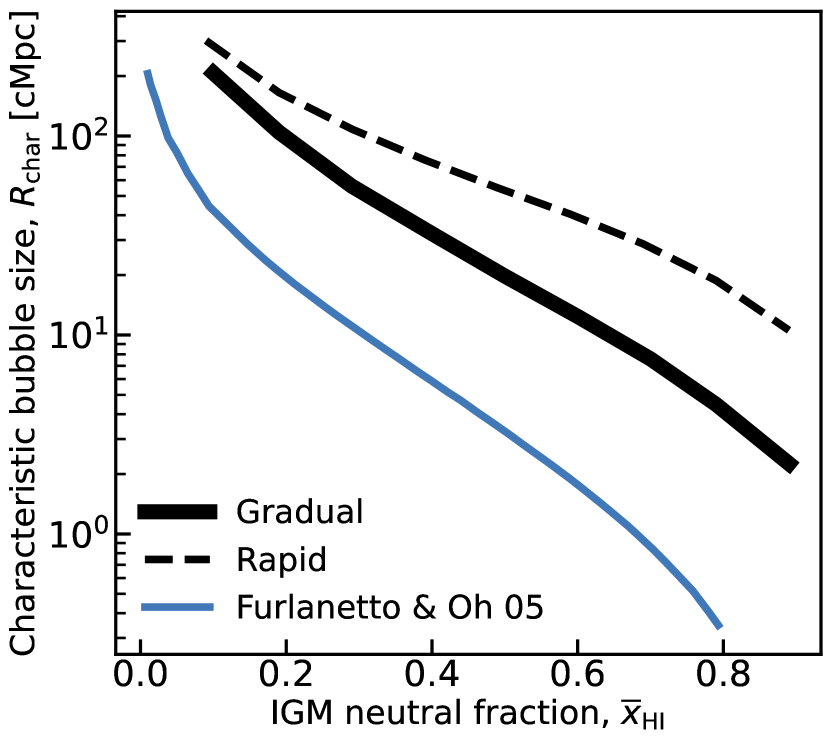
Figure 10: The evolution of ‘characteristic’ bubble sizes as a function of $\overline{x}_{\textsc{hi}}$ for our simulations compared to previous work. We show the mean size of ionised regions in this work (black) for the Gradual and Rapid models (solid and dashed lines respectively), and the characteristic size of ionised region in Furlanetto & Oh (2005) (blue). As discussed in Section 3.3, characteristic sizes of ionised regions in the Rapid model are much larger than those in the Gradual model at fixed $\overline{x}_{\textsc{hi}}$ . The excursion set formalism used by Furlanetto & Oh (2005) can underestimate the sizes of ionised regions by over an order of magnitude as it does not account for overlapping regions.

In this work, we characterise the bubble size distributions around typically observed reionisation-era galaxies for the first time over the full timeline of reionisation. Previously, only the total bubble size distribution has been modelled as a function of the neutral fraction (e.g. Furlanetto & Oh, 2005; Mesinger & Furlanetto, 2007; McQuinn et al., 2007a; Seiler et al., 2019).

In principle, the full bubble size distribution measured in this work should agree with previous works of similar reionisation setups. However, as seen in Figure 10 our mean bubble size is significantly larger than the characteristic bubble size modelled by Furlanetto & Oh (2005). Our bigger size comes from our use of the mean-free-path (MFP) method which is capable of taking into account the size of overlapped bubbles. The Furlanetto & Oh (2005) model underestimates the typical bubble size because they calculate bubbles via the excursion set formalism: as found by Lin et al. (2016), this method can underestimate bubble sizes by an order of magnitude. Our mean bubble size is comparable to those in works which use the mean free path approximation (e.g., Mesinger & Furlanetto, 2007; Seiler et al., 2019), modulo minor differences due to different assumptions for the ionising source population, as expected looking at the difference between our Gradual and Rapid models.

Other works have explored the correlation between ionised bubble size and galaxy luminosity. For example, Geil et al. (2017) and Qin et al. (2022) presented results from the DRAGONS simulation (Poole et al., 2016), finding more luminous galaxies are more likely to reside in large ionised bubbles, and that UV-faint galaxies have a large scatter in their host bubble size, consistent with our results in Section 3.1. However, these works only investigated a single redshift, IGM neutral fraction and reionising source model. Furthermore, the DRAGONS simulation is only (100 cMpc)³, meaning that it does not contain large numbers of rare overdensities and UV-bright galaxies (it contains only 2 galaxies as bright as GNz11, Mutch et al., 2016) and thus their predicted bubble sizes around UV-bright galaxies were subject to substantial Poisson noise. Yajima et al. (2018) presented a model for the sizes of ionised bubbles around galaxies by modelling cosmological Stromgren spheres around each galaxy (e.g., Shapiro & Giroux, 1987; Cen & Haiman, 2000), finding more massive and highly star-forming galaxies (and therefore more luminous) lie in larger ionised bubbles than low mass galaxies. However, this model does not take into account the overlapping of ionised regions, which can happen very early during reionisation (e.g., Lin et al., 2016) and thus their bubble sizes will be underestimated.

Our results in Section 3.1 highlight the importance of considering the expected ionised bubble size as a function of $M_{\textsc{uv}}$ calculated using the MFP method. Previous works which used the characteristic bubble size predicted by Furlanetto & Oh (2005) will thus be underestimating the size of ionised bubbles around observed galaxies at fixed neutral fraction. Jung et al. (2020) estimated the ionised bubble size required to explain the drop in Ly$\alpha$ transmission in the GOODS-N field at $z\sim 7.6$, and compared this bubble size to the Furlanetto & Oh (2005) characteristic bubble size as a function of neutral fraction to estimate ${\overline{x}_{\textsc{hi}}}\sim 0.49\pm 0.19$. Our results in Figure 10 imply that this approach will lead to an underestimate in $\overline{x}_{\textsc{hi}}$ . This likely explains the discrepancy between the neutral fraction estimated by Jung et al. (2020) and that inferred by Bolan et al. (2022) (${\overline{x}_{\textsc{hi}}}=0.83_{-0.11}^{+0.08}$) at a similar redshift, which was obtained by sampling sightlines in inhomogeneous IGM simulations.

4.2 Implications for the reionisation history and identification of primary ionising sources

Our results demonstrate that the visibility of Ly$\alpha$  emission at $z>8$ is unexpected given our consensus timeline for reionisation. The visibility of Ly$\alpha$  therefore implies some missing aspect in our understanding of reionisation.

As discussed in Section 3.4 there are three possibilities: (1) $\overline{x}_{\textsc{hi}}$ is lower than previously inferred; (2) reionisation is dominated by rarer sources providing larger, rarer bubbles; (3) these galaxies have high intrinsic Ly$\alpha$ production (Stark et al., 2017; Tang et al., 2023) and facilitated transmission in the IGM if the Ly$\alpha$ flux is emitted redward of systemic (e.g., Dijkstra et al., 2011; Mason et al., 2018b). These scenarios should be testable with spectroscopic observations in the field of high redshift Ly$\alpha$ -emitters. The most important first step is confirming if the large regions really are ionised. As the Ly$\alpha$ damping wing due to nearby neutral gas strongly attenuates Ly$\alpha$ close to systemic velocity, detecting Ly$\alpha$ with high escape fraction (estimated from Balmer lines) and very low velocity offset would be a key test to infer if the sources lie in large ionised regions. The $z>8$ LAEs that have been detected so far have Ly$\alpha$ velocity offset $>300$ km s^-1 (Tang et al., 2023; Bunker et al., 2023), thus the large ionised regions cannot be confirmed, but spectroscopy of the fainter galaxies (which are more likely to emit Ly$\alpha$ closer to systemic velocity, Prieto-Lyon et al., 2023) in these overdensities could be used to confirm large bubbles. These observations are now possible with JWST/NIRSpec, which can also importantly spectroscopically confirm overdensities. Excitingly, recent observations have discovered strong Ly$\alpha$ at low velocity offsets at $z>7$, implying large ionised regions (Tang et al., 2023; Saxena et al., 2023), and we will discuss quantitative constraints on the sizes of ionised regions in a future work.

We have also shown the bubble size distribution around observable galaxies depends on both the average IGM neutral fraction $\overline{x}_{\textsc{hi}}$ and the reionising source model. As the characteristic bubble size evolves strongly with $\overline{x}_{\textsc{hi}}$ (Figure 10), we may be able to constrain the reionisation history by simply counting overdensities of LAEs as a function of redshift. Trapp et al. (2022) recently used observed overdensities of LAEs to place joint constraints on the IGM neutral fraction and underlying matter density of those regions. That work is complementary to our approach in that it demonstrates a strong link between the overdensity of a region and the expected size of the ionised region around an overdensity.

In Sections 3.3 and  3.5 we show that the reionising source models have a strong impact on the predicted number of galaxies in large ionised bubbles early in reionisation. Finding evidence for a high number density of large ionised regions ($\,\hbox to0.0pt{\lower 3.5pt\hbox{$\mathchar 0\relax\sim$}\hss}\raise 1.0pt\hbox{$>$}\,10$ cMpc) at high redshift would thus provide evidence for reionisation driven by rare, bright sources. However, it is clear from our work that characteristic bubble sizes in different reionisation models at different $\overline{x}_{\textsc{hi}}$ can be degenerate, so focusing purely on observing overdensities likely to reside ionised regions will not be able to break this degeneracy.

As seen clearly in Figure 1, the Rapid model is characterised by biased, isolated large bubbles, thus it is much more likely that galaxies outside of overdensities will still be in mostly neutral regions early in reionisation in this scenario (see Figure 6). Thus to measure $\overline{x}_{\textsc{hi}}$ and fully break the degeneracy between reionisation morphologies requires observing a range of environments over time during reionisation. For example, observing the Ly$\alpha$ transmission from multiple sightlines to galaxies at different redshifts (e.g., Mesinger & Furlanetto, 2008b; Mason et al., 2018c; Whitler et al., 2020; Bolan et al., 2022) and the 21-cm power spectrum as a function of redshift (e.g., Furlanetto et al., 2004a; Geil et al., 2016).

5 Conclusions

We have produced large-scale (1.6 Gpc)³ simulations of the reionising IGM using 21cmfast and explored the size distribution of ionised bubbles around observable galaxies. Our conclusions are as follows:

1. Observable galaxies (${M_{\textsc{uv}}}<-16$) and galaxy overdensities are much less likely to reside in neutral regions compared to regions at the mean density. This is because galaxies are the source of reionisation.

2. The bubble size distribution around UV-bright (${M_{\textsc{uv}}}<-20$) galaxies and strong galaxy overdensities is biased to larger characteristic sizes compared to those in the full volume.

3. At all stages of reionisation we find a trend of increasing characteristic host bubble size and decreasing bubble size scatter with increasing UV luminosity and increasing overdensity.

4. As shown by prior works, we find the bubble size distribution strongly depends on both the IGM neutral fraction and the reionising source model. The difference between these models is most apparent in the early stages of reionisation, ${\overline{x}_{\textsc{hi}}}>0.5$: if numerous faint galaxies drive reionisation, we expect a gradual reionisation with numerous small bubbles, whereas if bright galaxies drive reionisation we expect a more rapid process characterised by larger bubbles biased around only the most overdense regions, with sizes $>30$ cMpc even in a 90% neutral IGM.

5. We use our simulations to interpret recent observations of galaxy overdensities detected with and without Ly$\alpha$ emission at $z\gtrsim 7$. We find the probability of finding a large ionised region with ${R_{\mathrm{ion}}}>1$ pMpc, capable of transmitting significant Ly$\alpha$ flux, at $z\approx 7-8$ is high ($\,\hbox to0.0pt{\lower 3.5pt\hbox{$\mathchar 0\relax\sim$}\hss}\raise 1.0pt\hbox{$>$}\,40-93$%) for large-scale galaxy overdensities, implying that Ly$\alpha$ -emitting galaxies detected at these redshifts are very likely to be in large ionised regions.

6. We find a very low probability of the $z\approx 8.7$ association of Ly$\alpha$ emitters in the EGS field and the $z=10.6$ galaxy GNz11, also detected with Ly$\alpha$ emission, to be in a large ionised bubble ($\sim 11\%$ and $\sim 7\%$, respectively). The Ly$\alpha$ detections at such a high redshift could be explained by either: a lower neutral fraction (${\overline{x}_{\textsc{hi}}}\lesssim 0.8$) than previously inferred; or if UV bright galaxies drive reionisation, which would produce larger bubbles; or if the intrinsic Ly$\alpha$ production in these galaxies is unusually high.

7. We make forecasts for the number density of ionised bubbles as a function of bubble size expected in the JWST COSMOS-Web survey and the Euclid Deep survey. Our fiducial model predicts no ionised regions $>10$ cMpc in the COSMOS-Web volume unless ${\overline{x}_{\textsc{hi}}}<0.9$, with tens of large bubbles expected by ${\overline{x}_{\textsc{hi}}}<0.7$, though with large cosmic variance. We find Euclid and Roman wide-area surveys will have sufficient volume to cover the size distribution of ionised regions with minimal cosmic variance and should be able to detect the UV-bright galaxies which signpost overdensities. Deeper photometric and spectroscopic follow-up around UV-bright galaxies in these surveys to confirm overdensities and Ly$\alpha$ emission could be used to infer $\overline{x}_{\textsc{hi}}$ and discriminate between reionisation models.

Our simulations show that in interpreting observations of $z>6$ galaxies it is important to consider the galaxy environment. We showed the bubble size distribution around observable galaxies and galaxy overdensities can be significantly shifted from the bubble size distribution over the whole cosmic volume. This motivates using realistic inhomogeneous reionisation simulations, or at least tailored bubble size distributions to interpret observations.

Our results imply that the early stages of reionisation are still very uncertain. Identifying and confirming large ionised regions at very high redshift is a first step to understanding these early stages, and thus the onset of star formation. This is now possible with deep JWST/NIRSpec observations which could map the regions around $z>8$ Ly$\alpha$ emitters. The detection of Ly$\alpha$ with high escape fraction and low velocity offset from other galaxies in the observed $z>8$ overdensities could confirm whether the Ly$\alpha$  emitters at $z>8$ are tracing unexpectedly large ionised regions (e.g., Tang et al., 2023; Saxena et al., 2023).

Data Availability

Tables of bubble sizes as a function of $\overline{x}_{\textsc{hi}}$ , $M_{\textsc{uv}}$ , and galaxy overdensity (using the same volume as in Section 3.2) are publicly available here: https://github.com/ting-yi-lu/bubble_size_overdensities_paper.
Bubble size distributions around other overdensities can be distributed upon reasonable request to the authors.

Appendix A Model UV luminosity function

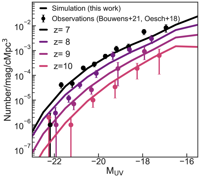
Figure 11: UV luminosity functions from our model at $z\sim 7,8,9$ (solid lines) in comparison to HST measurements of the UV LF by Bouwens et al. (2021) ($z=7-9$) and Oesch et al. (2018) ($z=10$).

In Figure 11 we demonstrate that our model for assigning UV magnitudes to simulated halos (Section 2.2) reproduces observed UV luminosity functions over $z\sim 7-10$ as required for our study. We note the apparent turnover at ${M_{\textsc{uv}}}\,\hbox to0.0pt{\lower 3.5pt\hbox{$\mathchar 0\relax\sim$}\hss}\raise 1.0pt\hbox{$>$}\,-16$ is not physical, but arises due to enforcing a halo mass cut-off at $M_{\rm halo}=5\times 10^{9}M_{\odot}$ in our catalogue due to memory restrictions.

Appendix B Bubble size distributions at different redshifts

Figure 12: Bubble size distributions, $dp/d\log_{10}R$ , as a function of redshift for $z=7$ (solid lines) and $z=8$ (dashed lines) and $z=9$ (dotted lines) for ${M_{\textsc{uv}}}=-16,-22$ at ${\overline{x}_{\textsc{hi}}}=0.5$. We also show the total bubble size distribution as a thick grey line in each redshift. We see a minimal difference at different redshifts, but higher redshifts show slighter higher bubble sizes as we discuss in Appendix B.

Here we compare the bubble size distributions at $z=7-9$. We show the bubble size distributions at ${\overline{x}_{\textsc{hi}}}=0.5$ for each redshift in Figure 12. We see negligible differences as a function of redshift, but that bubble sizes are slightly larger at fixed neutral fraction at higher redshift. This is because we use a fixed halo mass cut-off to calculate the ionising emissivity (as described in Section 2.1), and at higher redshifts the same mass halo will be more biased, resulting in rarer, larger bubbles at fixed $\overline{x}_{\textsc{hi}}$ as in our Rapid model. However, the difference between the bias of halos of fixed mass and different redshifts is much lower than the difference between the bias due to our two mass thresholds for the Gradual and Rapid model, so this redshift effect is minimal.

Appendix C Bubble size distribution models for observed overdensities

In Figure 13 we show the bubble size distribution for the observed overdensities described in Section 3.4. In all plots we show the bubble size distribution in the full volume in the neutral fraction range expected given current constraints on reionisation (Mason et al., 2019b), and the bubble size distribution in regions as overdense as those observed.

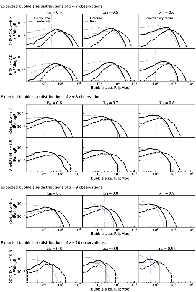
Figure 13: Bubble size distributions for the same overdensity observation setups as the COSMOS (top panel), BDF (second panel), EGS_z8 (third panel), Abell2744 (fourth panel), EGS_z9 (fifth panel), and GOODS-N (bottom panel), at the IGM neutral fractions expected at these redshifts (Mason et al., 2019b), from the Gradual (solid) and Rapid (dashed) models. The bubble size estimated by previous works (Endsley et al., 2022; Castellano et al., 2016; Leonova et al., 2022; Morishita et al., 2022; Jung et al., 2022; Tacchella et al., 2023) are marked with purple vertical lines. A summary of our simulation setup is given in Table 1.

References

- Adelberger et al. (1998) Adelberger K. L., Steidel C. C., Giavalisco M., Dickinson M., Pettini M., Kellogg M., 1998, ApJ, 505, 18
- Akeson et al. (2019) Akeson R., et al., 2019, arXiv e-prints, p. arXiv:1902.05569
- Barone-Nugent et al. (2014) Barone-Nugent R. L., et al., 2014, ApJ, 793, 17
- Bolan et al. (2022) Bolan P., et al., 2022, MNRAS, 517, 3263
- Bosman et al. (2022) Bosman S. E. I., et al., 2022, MNRAS, 514, 55
- Bouwens et al. (2021) Bouwens R. J., et al., 2021, AJ, 162, 47
- Bruton et al. (2023) Bruton S., Lin Y.-H., Scarlata C., Hayes M. J., 2023, arXiv e-prints, p. arXiv:2303.03419
- Bunker et al. (2023) Bunker A. J., et al., 2023, arXiv e-prints, p. arXiv:2302.07256
- Casey et al. (2022) Casey C. M., et al., 2022, arXiv e-prints, p. arXiv:2211.07865
- Cassata et al. (2015) Cassata P., et al., 2015, A&A, 573, A24
- Castellano et al. (2016) Castellano M., et al., 2016, ApJ, 818, L3
- Castellano et al. (2018) Castellano M., et al., 2018, ApJ, 863, L3
- Castellano et al. (2022) Castellano M., et al., 2022, p. arXiv:2207.09436
- Cen & Haiman (2000) Cen R., Haiman Z., 2000, ApJ, 542, L75
- Cole & Kaiser (1989) Cole S., Kaiser N., 1989, MNRAS, 237, 1127
- Cooray & Milosavljevic (2005) Cooray A., Milosavljevic M., 2005, ApJ, 627, 4
- Davies et al. (2018a) Davies F. B., Becker G. D., Furlanetto S. R., 2018a, ApJ, 860, 155
- Davies et al. (2018b) Davies F. B., et al., 2018b, ApJ, 864, 142
- Dayal & Ferrara (2018) Dayal P., Ferrara A., 2018, Phys. Rep., 780, 1
- Dijkstra (2014) Dijkstra M., 2014, Publ. Astron. Soc. Australia, 31, e040
- Dijkstra et al. (2011) Dijkstra M., Mesinger A., Wyithe J. S. B., 2011, MNRAS, 414, 2139
- Endsley & Stark (2022) Endsley R., Stark D. P., 2022, MNRAS, 511, 6042
- Endsley et al. (2021) Endsley R., Stark D. P., Chevallard J., Charlot S., 2021, MNRAS, 500, 5229
- Endsley et al. (2022) Endsley R., Stark D. P., Whitler L., Topping M. W., Chen Z., Plat A., Chisholm J., Charlot S., 2022, arXiv e-prints, p. arXiv:2208.14999
- Euclid Collaboration et al. (2022) Euclid Collaboration et al., 2022, A&A, 662, A112
- Finkelstein et al. (2019) Finkelstein S. L., et al., 2019, arXiv:1902.02792 [astro-ph]
- Furlanetto & Oh (2005) Furlanetto S. R., Oh S. P., 2005, MNRAS, 363, 1031
- Furlanetto et al. (2004a) Furlanetto S. R., Hernquist L., Zaldarriaga M., 2004a, MNRAS, 354, 695
- Furlanetto et al. (2004b) Furlanetto S. R., Zaldarriaga M., Hernquist L., 2004b, ApJ, 613, 1
- Geil et al. (2016) Geil P. M., Mutch S. J., Poole G. B., Angel P. W., Duffy A. R., Mesinger A., Wyithe J. S. B., 2016, MNRAS, 462, 804
- Geil et al. (2017) Geil P. M., Mutch S. J., Poole G. B., Duffy A. R., Mesinger A., Wyithe J. S. B., 2017, MNRAS, 472, 1324
- Greig & Mesinger (2017) Greig B., Mesinger A., 2017, MNRAS, 465, 4838
- Greig et al. (2019) Greig B., Mesinger A., Bañados E., 2019, MNRAS, 484, 5094
- Grogin et al. (2011) Grogin N. A., et al., 2011, ApJS, 197, 35
- Hassan et al. (2018) Hassan S., Davé R., Mitra S., Finlator K., Ciardi B., Santos M. G., 2018, MNRAS, 473, 227
- Hoag et al. (2019) Hoag A., et al., 2019, ApJ, 878, 12
- Hu et al. (2021) Hu W., et al., 2021, Nature Astronomy, 5, 485
- Hutter et al. (2015) Hutter A., Dayal P., Müller V., 2015, MNRAS, 450, 4025
- Hutter et al. (2017) Hutter A., Dayal P., Müller V., Trott C. M., 2017, ApJ, 836, 176
- Hutter et al. (2021) Hutter A., Dayal P., Yepes G., Gottlöber S., Legrand L., Ucci G., 2021, MNRAS, 503, 3698
- Ishigaki et al. (2016) Ishigaki M., Ouchi M., Harikane Y., 2016, ApJ, 822, 5
- Jung et al. (2020) Jung I., et al., 2020, ApJ, 904, 144
- Jung et al. (2022) Jung I., et al., 2022, arXiv e-prints, p. arXiv:2212.09850
- Kaur et al. (2020) Kaur H. D., Gillet N., Mesinger A., 2020, arXiv:2004.06709 [astro-ph]
- Kimm & Cen (2014) Kimm T., Cen R., 2014, ApJ, 788, 121
- Koekemoer et al. (2011) Koekemoer A. M., et al., 2011, ApJS, 197, 36
- Kullback (1968) Kullback S., 1968, Inc., NY
- Larson et al. (2022) Larson R. L., et al., 2022, ApJ, 930, 104
- Larson et al. (2023) Larson R. L., et al., 2023, arXiv e-prints, p. arXiv:2303.08918
- Leonova et al. (2022) Leonova E., et al., 2022, MNRAS, 515, 5790
- Lewis et al. (2020) Lewis J. S. W., et al., 2020, MNRAS, 496, 4342
- Lidz et al. (2009) Lidz A., Zahn O., Furlanetto S. R., McQuinn M., Hernquist L., Zaldarriaga M., 2009, ApJ, 690, 252
- Lin et al. (2016) Lin Y., Oh S. P., Furlanetto S. R., Sutter P. M., 2016, MNRAS, 461, 3361
- Lu et al. (2022) Lu T.-Y., et al., 2022, MNRAS, 517, 1264
- Ma et al. (2020) Ma X., Quataert E., Wetzel A., Hopkins P. F., Faucher-Giguère C.-A., Kereš D., 2020, MNRAS, 498, 2001
- Malhotra & Rhoads (2006) Malhotra S., Rhoads J. E., 2006, ApJ, 647, L95
- Malkan et al. (2021) Malkan M. A., et al., 2021, PASSAGE-Parallel Application of Slitless Spectroscopy to Analyze Galaxy Evolution, JWST Proposal. Cycle 1, ID. #1571
- Mason & Gronke (2020) Mason C. A., Gronke M., 2020, MNRAS, 499, 1395
- Mason et al. (2015) Mason C. A., Trenti M., Treu T., 2015, ApJ, 813, 21
- Mason et al. (2018a) Mason C. A., Treu T., Dijkstra M., Mesinger A., Trenti M., Pentericci L., de Barros S., Vanzella E., 2018a, ApJ, 856, 2
- Mason et al. (2018c) Mason C. A., et al., 2018c, ApJ, 857, L11
- Mason et al. (2018b) Mason C. A., et al., 2018b, ApJ, 857, L11
- Mason et al. (2019a) Mason C. A., et al., 2019a, MNRAS, 485, 3947
- Mason et al. (2019b) Mason C. A., Naidu R. P., Tacchella S., Leja J., 2019b, MNRAS, 489, 2669
- Mason et al. (2023) Mason C. A., Trenti M., Treu T., 2023, MNRAS,
- McGreer et al. (2015) McGreer I. D., Mesinger A., D’Odorico V., 2015, MNRAS, 447, 499
- McQuinn et al. (2007a) McQuinn M., Lidz A., Zahn O., Dutta S., Hernquist L., Zaldarriaga M., 2007a, MNRAS, 377, 1043
- McQuinn et al. (2007b) McQuinn M., Hernquist L., Zaldarriaga M., Dutta S., 2007b, MNRAS, 381, 75
- Mesinger (2019) Mesinger A., 2019, The Cosmic 21-cm Revolution; Charting the first billion years of our universe, doi:10.1088/2514-3433/ab4a73.
- Mesinger & Furlanetto (2007) Mesinger A., Furlanetto S., 2007, ApJ, 669, 663
- Mesinger & Furlanetto (2008a) Mesinger A., Furlanetto S. R., 2008a, MNRAS, 385, 1348
- Mesinger & Furlanetto (2008b) Mesinger A., Furlanetto S. R., 2008b, MNRAS, 386, 1990
- Mesinger et al. (2011) Mesinger A., Furlanetto S., Cen R., 2011, MNRAS, 411, 955
- Mesinger et al. (2015) Mesinger A., Aykutalp A., Vanzella E., Pentericci L., Ferrara A., Dijkstra M., 2015, MNRAS, 446, 566
- Mesinger et al. (2016a) Mesinger A., Greig B., Sobacchi E., 2016a, MNRAS, 459, 2342
- Mesinger et al. (2016b) Mesinger A., Greig B., Sobacchi E., 2016b, MNRAS, 459, 2342
- Miralda-Escude (1998) Miralda-Escude J., 1998, ApJ, 501, 15
- Miralda-Escudé et al. (2000) Miralda-Escudé J., Haehnelt M., Rees M. J., 2000, ApJ, 530, 1
- Mo et al. (1997) Mo H. J., Jing Y. P., White S. D. M., 1997, MNRAS, 284, 189
- Morales & Wyithe (2010) Morales M. F., Wyithe J. S. B., 2010, ARA&A, 48, 127
- Morishita et al. (2022) Morishita T., et al., 2022, arXiv e-prints, p. arXiv:2211.09097
- Mutch et al. (2016) Mutch S. J., et al., 2016, MNRAS, 8, 1
- Naidu et al. (2020) Naidu R. P., Tacchella S., Mason C. A., Bose S., Oesch P. A., Conroy C., 2020, ApJ, 892, 109
- Ocvirk et al. (2020) Ocvirk P., et al., 2020, MNRAS, 496, 4087
- Oesch et al. (2015) Oesch P. A., et al., 2015, ApJ, 804, L30
- Oesch et al. (2016) Oesch P. A., et al., 2016, ApJ, 819, 129
- Oesch et al. (2018) Oesch P. A., Bouwens R. J., Illingworth G. D., Labbe I., Stefanon M., 2018, ApJ, 855, 105
- Ouchi et al. (2017) Ouchi M., et al., 2017, PASJ, 00, 1
- Overzier et al. (2006) Overzier R. A., et al., 2006, ApJ, 637, 58
- Park et al. (2014) Park J., Kim H.-S., Wyithe J. S. B., Lacey C. G., 2014, MNRAS, 438, 2474
- Park et al. (2021) Park H., et al., 2021, ApJ, 922, 263
- Planck Collaboration et al. (2020) Planck Collaboration et al., 2020, A&A, 641, A6
- Pober et al. (2014) Pober J. C., et al., 2014, ApJ, 782, 66
- Poole et al. (2016) Poole G. B., Angel P. W., Mutch S. J., Power C., Duffy A. R., Geil P. M., Mesinger A., Wyithe S. B., 2016, MNRAS, 459, 3025
- Prieto-Lyon et al. (2023) Prieto-Lyon G., et al., 2023, arXiv e-prints, p. arXiv:2304.02666
- Qin et al. (2021) Qin Y., Mesinger A., Bosman S. E. I., Viel M., 2021, MNRAS, 506, 2390
- Qin et al. (2022) Qin Y., Wyithe J. S. B., Oesch P. A., Illingworth G. D., Leonova E., Mutch S. J., Naidu R. P., 2022, MNRAS, 510, 3858
- Ren et al. (2018) Ren K., Trenti M., Mutch S. J., 2018, ApJ, 856, 81
- Ren et al. (2019) Ren K., Trenti M., Mason C. A., 2019, ApJ, 878, 114
- Roberts-Borsani et al. (2016) Roberts-Borsani G. W., et al., 2016, ApJ, 823, 143
- Roberts-Borsani et al. (2022) Roberts-Borsani G., et al., 2022, arXiv e-prints, p. arXiv:2207.01629
- Robertson (2010) Robertson B. E., 2010, ApJ, 716, L229
- Santos (2004) Santos M. R., 2004, MNRAS, 349, 1137
- Saxena et al. (2023) Saxena A., et al., 2023, arXiv e-prints, p. arXiv:2302.12805
- Seiler et al. (2019) Seiler J., Hutter A., Sinha M., Croton D., 2019, MNRAS, 487, 5739
- Shapiro & Giroux (1987) Shapiro P. R., Giroux M. L., 1987, ApJ, 321, L107
- Sheth et al. (2001) Sheth R. K., Mo H. J., Tormen G., 2001, MNRAS, 323, 1
- Sobacchi & Mesinger (2014) Sobacchi E., Mesinger A., 2014, MNRAS, 440, 1662
- Sobacchi & Mesinger (2015) Sobacchi E., Mesinger A., 2015, MNRAS, 453, 1843
- Stark (2016) Stark D. P., 2016, ARA&A, 54, 761
- Stark et al. (2010) Stark D. P., Ellis R. S., Chiu K., Ouchi M., Bunker A., 2010, MNRAS, 408, 1628
- Stark et al. (2011) Stark D. P., Ellis R. S., Ouchi M., 2011, ApJ, 728, L2
- Stark et al. (2017) Stark D. P., et al., 2017, MNRAS, 464, 469
- Tacchella et al. (2023) Tacchella S., et al., 2023, arXiv e-prints, p. arXiv:2302.07234
- Tang et al. (2023) Tang M., et al., 2023, arXiv e-prints, p. arXiv:2301.07072
- Tempel et al. (2009) Tempel E., Einasto J., Einasto M., Saar E., Tago E., 2009, A&A, 495, 37
- Tilvi et al. (2020) Tilvi V., et al., 2020, ApJ, 891, L10
- Trac & Cen (2007) Trac H., Cen R., 2007, ApJ, 671, 1
- Trapp et al. (2022) Trapp A. C., Furlanetto S. R., Davies F. B., 2022, Lyman-alpha Emitters in Ionized Bubbles: Constraining the Environment and Ionized Fraction (arXiv:2210.06504), doi:10.48550/arXiv.2210.06504
- Trebitsch et al. (2017) Trebitsch M., Blaizot J., Rosdahl J., Devriendt J., Slyz A., 2017, MNRAS
- Vanzella et al. (2011) Vanzella E., et al., 2011, ApJ, 730, L35
- Vincent & Soille (1991) Vincent L., Soille P., 1991, IEEE Transactions on Pattern Analysis & Machine Intelligence, 13, 583
- Wang et al. (2022) Wang Y., et al., 2022, ApJ, 928, 1
- Weinberger et al. (2018) Weinberger L. H., Kulkarni G., Haehnelt M. G., Choudhury T. R., Puchwein E., 2018, MNRAS, 479, 2564
- Whitler et al. (2020) Whitler L. R., Mason C. A., Ren K., Dijkstra M., Mesinger A., Pentericci L., Trenti M., Treu T., 2020, MNRAS, 495, 3602
- Wise et al. (2014) Wise J. H., Demchenko V. G., Halicek M. T., Norman M. L., Turk M. J., Abel T., Smith B. D., 2014, MNRAS, 442, 2560
- Xu et al. (2016) Xu H., Wise J. H., Norman M. L., Ahn K., O’Shea B. W., 2016, ApJ, 833, 84
- Yajima et al. (2018) Yajima H., Sugimura K., Hasegawa K., 2018, MNRAS, 477, 5406
- Yang et al. (2005) Yang X., Mo H. J., Jing Y. P., van den Bosch F. C., 2005, MNRAS, 358, 217
- Zackrisson et al. (2020) Zackrisson E., et al., 2020, MNRAS, 493, 855
- Zahn et al. (2007) Zahn O., Lidz A., McQuinn M., Dutta S., Hernquist L., Zaldarriaga M., Furlanetto S. R., 2007, ApJ, 654, 12
- Zitrin et al. (2015a) Zitrin A., et al., 2015a, ApJ, 801, 44
- Zitrin et al. (2015b) Zitrin A., et al., 2015b, ApJ, 810, L12
- van Mierlo et al. (2022) van Mierlo S. E., et al., 2022, A&A, 666, A200
- van der Walt et al. (2014) van der Walt S., et al., 2014, PeerJ, 2, e453