Curie-law crossover in spin liquids
Abstract
The Curie-Weiss law is widely used to estimate the strength of frustration in frustrated magnets. However, the Curie-Weiss law was originally derived as an estimate of magnetic correlations close to a mean-field phase transition, which – by definition – is absent in spin liquids. Instead, the susceptibility of spin liquids is known to undergo a Curie-law crossover between two magnetically disordered regimes. Here, we study the generic aspect of the Curie-law crossover by comparing a variety of frustrated spin models in two and three dimensions, using both classical Monte Carlo simulations and analytical Husimi tree calculations. Husimi tree calculations fit remarkably well the simulations for all temperatures and almost all lattices. We also propose a Husimi Ansatz for the reduced susceptibility , to be used in complement to the traditional Curie-Weiss fit in order to estimate the Curie-Weiss temperature . Applications to materials are discussed.
I Introduction
The Curie-Weiss law is a simple and useful tool to estimate the behavior of the susceptibility for conventional magnets at high temperatures Curie (1895); Weiss (1907); Kittel (2004); Ashcroft and Mermin (1976); Mugiraneza and Hallas (2022)
| (1) |
with the Curie constant, and the Curie-Weiss temperature. In a Landau mean-field treatment Landau (1937), represents the transition temperature. The sign of indicates dominant ferromagnetic () or antiferromagnetic () interactions, while the limit represents the susceptibility of a paramagnet, given by the Curie law, . For more details about the calculation of the Curie-Weiss law in susceptibility measurements, we refer the reader to the recent tutorial by Mugiraneza & Hallas [Mugiraneza and Hallas, 2022].
In frustrated magnets, the Curie-Weiss temperature is often used to measure the “frustration index” Ramirez (1994)
| (2) |
by comparing the transition, or freezing, temperature of a material, , to its mean-field expectation, , for an unfrustrated system. Large values of account for strong frustration in the system. For a spin liquid where theoretically, the frustration index diverges. Being a priori readily accessible to experiments, this quantity has become a convenient tool to gauge how frustrated a system is.
But as many successful, broadly used indicators, a few shortcomings are inevitable. Deviations from the standard Curie-Weiss law have been studied in a variety of magnetic systems, such as spin glasses Nagasawa (1967); Morgownik and Mydosh (1981), the pyrochlore molybdate Y2Mo2O7 Silverstein et al. (2014), the valence bond glass Ba2YMoO6 de Vries et al. (2010), or Kitaev materials with strong spin-orbit coupling Li et al. (2021), to cite but a few. For example in anisotropic lattices, the high-temperature Curie constant and low-temperature transition temperature may be set by different energy scales, giving rise to an artificially large parameter even when the system is barely frustrated Pohle et al. (2016); Schmidt and Thalmeier (2017).
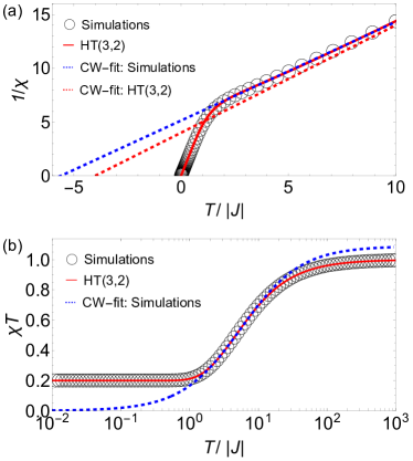
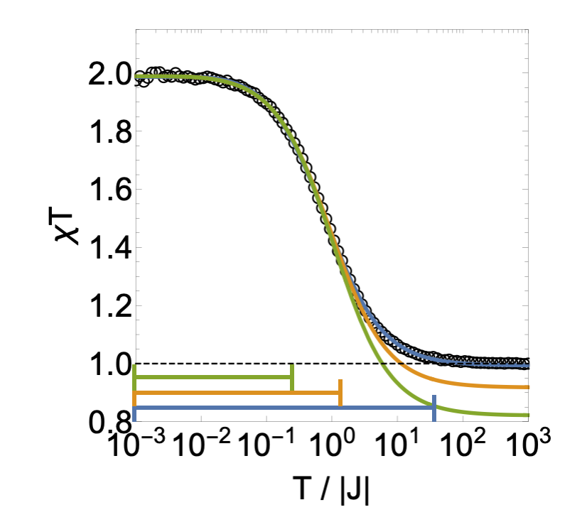
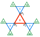
In spin liquids, this deviation has been rationalized as the onset of a Curie-law crossover Jaubert (2009); Jaubert et al. (2013) between the universal high-temperature Curie law and a low-temperature, model-specific, spin-liquid Curie law Isakov et al. (2004a); Isoda (2008); Macdonald et al. (2011); Jaubert et al. (2013). The problem is that fitting the susceptibility of spin liquids with a Curie-Weiss law always gives an answer, but not necessarily the right one, as illustrated for the Ising kagome antiferromagnet in Fig. 1. Beyond the traditional difficulties to measure the Curie-Weiss temperature Mugiraneza and Hallas (2022); Li et al. (2021), frustration precisely prevents the phase transition in spin liquids that would justify the Curie-Weiss fit as a mean-field approximation of a scaling law with critical exponent . Eq. (1) is only valid at high temperature as a first order perturbation of the Curie law. And whether this high-temperature regime is accessible to experiments then becomes an important question Mugiraneza and Hallas (2022); Li et al. (2021). Internal energy scales such as a single-ion crystal field, a band gap, the structural distortion of the lattice or even the melting of the materials might prevent access to the necessary high temperatures. In that case, the values of the Curie constant and Curie-Weiss temperature strongly depend on the temperature range of the fitting procedure Jaubert et al. (2013); Nag and Ray (2017). The latter can even change sign when the exchange coupling is particularly small (see e.g. Refs. [Bramwell et al., 2000; Lummen et al., 2008] for Dy2Ti2O7). And as a high-temperature expansion of the susceptibility, the Curie-Weiss fit is not designed to capture the spin-liquid behavior at low temperatures.
To summarise the issue, applying the Curie-Weiss fit to frustrated magnets means applying a method that has been derived around a mean-field critical point, to a class of systems where this critical point is absent by definition.
Our goal in this paper is to rationalise this conceptual divergence of viewpoints and to build a generic understanding of the Curie-law crossover in spin liquids. Is it possible to quantify how the magnetic susceptibility deviates from the Curie-Weiss law, not just for a specific model but for frustrated magnets in general ? In particular, can we identify generic features ? Practically, understanding the limits of the Curie-Weiss fit will help estimate the appropriate temperature window to measure the Curie-Weiss temperature, and what to do when this window is not experimentally available.
II Summary of results
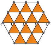
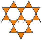
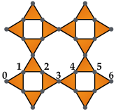
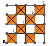
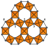
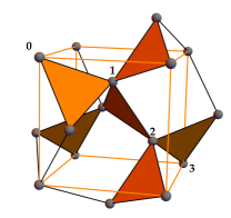
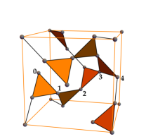
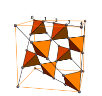
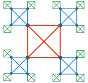
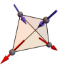
Since our goal is to build a generic picture of the Curie-law crossover for spin liquids, we will study a variety of frustrated lattices in two and three dimensions [Fig. 2], first considering Ising spins, then extending the analysis to include continuous Heisenberg spins, anisotropic exchange, and finally analyzing experimental data of materials with quantum spins. Our motivation here is not to study each model individually. That has already been done extensively in the literature; see e.g. the following references for the two dimensional triangular Stephenson (1964); Rastelli et al. (1977); Isoda (2008), kagome Garanin and Canals (1999); Macdonald et al. (2011), square-kagome Pohle et al. (2016); Jurčišinová and Jurčišin (2018); Richter et al. (2022), checkerboard Canals and Garanin (2002); Henley (2010) and ruby Rehn et al. (2017) lattices, and for the three dimensional trillium Redpath and Hopkinson (2010), hyperkagome Hopkinson et al. (2007), and pyrochlore Canals and Garanin (2001); Isakov et al. (2004a); Jaubert et al. (2013); Bovo et al. (2013, 2018) lattices. Instead, we will compare these models together, understand why similarities appear between some of them, and build an overall intuition for the phenomenon of the Curie-law crossover in spin liquids.
On the theoretical front, comparing unbiased classical Monte Carlo simulations to the analytical Husimi-Tree approximation shows that thermodynamic quantities are, to a large extent, independent of the lattice dimension, and even of the structure of the lattice beyond the minimal frustrated unit cells [Fig. 5]. What essentially matters is simply the type of frustrated unit cell (triangle, tetrahedron, …) and the local connectivity between them. In addition, we also show how to compute correlations on Husimi trees with a non-trivial distribution of sublattices and local easy-axes on trillium and hyperkagome lattices. [Appendix C.4].
On the experimental front, one of our take-home messages is that the reduced susceptibility (that is frequently used by chemists) is a very useful complement to the inverse susceptibility for frustrated magnets. The Curie-law crossover is especially transparent in this quantity, between two horizontal asymptotic lines. thus immediately tells us (i) how far we are from the high-temperature Curie law, and (ii) the presence or absence of a low-temperature spin-liquid Curie law. This is especially useful because some frustrated materials may ultimately order or freeze at a very low temperature . But if the reduced susceptibility reaches a low-temperature plateau at , then it is a solid indication that a strongly correlated regime characteristic of a spin liquid exists over a finite temperature window .
In order to describe the Curie-law crossover in its entirety, we introduce the following fitting Ansatz [Fig. 1(b)]:
| (3) |
inspired by the above analogy between disparate models and Husimi-tree calculations. This empirical Ansatz provides a complementary estimate of the Curie constant and Curie-Weiss temperature,
| (4) |
that is not based on a high-temperature expansion. Hence, if Eq. (4) agrees with values obtained from a Curie-Weiss fit, then it is reasonable to consider them as an accurate description of the material. On the other hand if there is a noticeable mismatch, then it is likely that experimental data have not reached the high-temperature regime where the Curie-Weiss law is valid.
The remainder of this Article is structured as follows. In Sec. III, we introduce the models of classical spin liquids, defined with Ising spins on a variety of frustrated lattices in two and three dimensions [Fig. 2]. These models will be solved numerically with classical Monte Carlo simulations and analytically on their corresponding Husimi trees [Fig. 3].
In Sec. IV, we present thermodynamic quantities for all spin liquids introduced in Sec III and discuss analogies and signatures of their Curie-law crossover. In particular, we discuss the reason for the very good match between Monte-Carlo simulations and Husimi-tree calculations, despite the different lattice structure.
In Sec. V, we discuss the limitations of the conventional Curie-Weiss fit, showing the advantage to use the reduced susceptibility . We introduce and benchmark the Husimi Ansatz [Eq. (3)] to numerical simulations of spin-liquid models with Ising and continuous Heisenberg spins.
In Sec. VI, we apply this Ansatz to experimental data for the pyrochlore NaCaNi2F7 [Krizan and Cava, 2015], the square-kagome KCu6AlBiO4(SO4)5Cl [Fujihala et al., 2020] and the spiral spin liquid FeCl3 [Gao et al., 2022].
In Sec. VII, we conclude with a brief summary and implications for future experiments on spin liquid materials.
Details on the lattice geometries, Monte Carlo simulations, Husimi tree calculations, connection to Coulomb gauge field theory, and structure factors are given in Appendices A, B, C, D and E respectively.
III Models and methods
III.1 The Ising model
In Sec. III and IV, we focus on thermodynamic properties of minimal spin-liquid models,
| (5) |
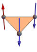
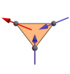
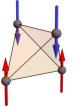
for Ising spins , with , and nearest-neighbour coupling , applied to a variety of lattices, as shown in Fig. 2. We shall consider two types of Ising spins, either collinear along the same global -axis , or oriented along their local easy axis attached to the sublattice of site . The latter is motivated from single-ion anisotropy, as found, for example, in kagome materials like Dy3Mg2Sb3O14 Paddison et al. (2016) and spin ices like Dy2Ti2O7 and Ho2Ti2O7 on the pyrochlore lattice Bramwell and Harris (2020); Udagawa and Jaubert (2021), and EuPtSi Adroja et al. (1990); Hopkinson and Kee (2006); Redpath and Hopkinson (2010) on the trillium lattice. We shall refer to each system as “global-axis” and “local-axis” models, as illustrated in Fig. 4. All local easy axes relevant for this work are defined in Appendix A. Global-axis and local-axis models are equivalent, up to a simple rescaling of the coupling constant Bramwell and Harris (1998); Moessner and Chalker (1998a)
| (6) |
where and are two neighbouring sites. For lattices considered here, the scalar product is the same for all neighbouring pairs, which means that the energy, specific heat and entropy of the two models are the same up to rescaling (6). However, magnetic quantities such as the susceptibility differ. In this work, the exchange coupling is always antiferromagnetic (ferromagnetic ) for global-axis (local-axis) models, in order to stabilise a spin-liquid ground state. From now on, all energies and temperatures are given in units of , understanding that the rescaling of Eq. (6) is always applied for local-axis models.
local axis
| Lattice | S | ||||
| Monte Carlo | Husimi Tree | other methods | Monte Carlo | Husimi Tree | |
| kagome | Wills et al. (2002) | Kanô and Naya (1953) | 1.988(1) | 2 | |
| hyperkagome | Wills et al. (2002) | n/a | 1.500(1) | 3/2 | |
| square-kagome | Pohle et al. (2016) | Pohle et al. (2016) | n/a | ||
| triangular | Redpath and Hopkinson (2010) | ||||
| trillium | Redpath and Hopkinson (2010) | Redpath and Hopkinson (2010) | n/a | 0.969(1) | 1 |
| ruby | Pauling (1935) | n/a | |||
| checkerboard | 0.216(1) | Lieb (1967) | 0.0 | ||
| pyrochlore | 0.205006(9) Nagle (1966) | 2.002(1)Isakov et al. (2004a) | 2 | ||
III.2 Spin liquids on the Husimi tree
The frustrated Ising model [Eq. (5)] on corner-sharing lattices [see Fig. 2] can be solved, regardless of its physical dimension, by numerical methods such as classical Monte Carlo simulations [see Appendix B]. On the analytical front, however, the question is more delicate. Since correlations play a major role, one needs a method beyond standard mean-field theory, but nonetheless valid for frustrated models across different dimensions. The Husimi-Tree (HT) calculation precisely fits our needs, by incorporating the local frustrated constraints of the lattice, irrespectively of its dimension. HT recursively extends from a central frustrated cell – e.g. a triangle or a tetrahedron – into a non-reciprocal lattice, without any internal loop beyond the frustrated cell [Fig. 3]. As a consequence, its boundary is of comparable size to the volume of the bulk Bethe (1935); Baxter (1982) and the HT remains a mean-field approach. It is thus inaccurate at critical points, except above their upper critical dimensions Wada and Ogawa (1998); Jaubert et al. (2008, 2010). But since we explicitly study models away from phase transitions, we expect pertinent analytical insights from the HT, spurred on by encouraging results on frustrated systems in the literature Wada and Ogawa (1998); Monroe (1998a); ichi Yoshida et al. (2002); Jaubert et al. (2008, 2009, 2010); Udagawa et al. (2010); Jaubert et al. (2013); Jurčišinová and Jurčišin (2014); Jurčišinová et al. (2014a, b). Technical aspects of the HT method are explained in Appendix C including the explicit expressions of the thermodynamic quantities and how to include the non-collinear easy-axes of the different sublattices.
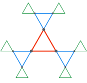
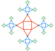
We will compare a variety of physical lattices, with different numbers of internal loops and frustrated unit cells [Fig. 2], to their pseudo-lattice counterparts on the Husimi tree, which do not have any internally closed loops [Fig. 3]. Let us define as the smallest internal loop formed by frustrated cells on the physical lattice. We relate all physical lattices, as introduced in Fig. 2, to their corresponding HT trees, according to the number of sites per frustrated cell and their connectivity:
-
(i)
HT(3,2) [Fig. 3(a)] contains three sites in the frustrated cell, where each site is connected between two cells. It relates to the kagome (), square-kagome () and hyperkagome () lattice. Considering the complexity of the frustrated cell in the square-kagome lattice, we also included the Husimi tree HTS [Fig. 3(b)] to improve the mean-field approximation.
-
(ii)
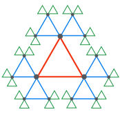
HT(3,3) [Fig. 3(c)] contains three sites in the frustrated cell, where each site is connected between three cells, and relates to the triangular () and trillium () lattice.
-
(iii)
HT(4,2) [Fig. 3(d)] contains four sites in the frustrated cell, where each site is connected between two cells, and relates to the checkerboard (), ruby () and pyrochlore () lattice.
The similarity between a given lattice and its Husimi tree, taken individually, makes sense – except maybe for the triangular lattice, which will be discussed separately in Section IV.4. In this set up we shall investigate the Curie-law crossover by comparing thermodynamic quantities between the physical lattice (as obtained by classical Monte Carlo simulations) and their corresponding pseudo lattice on the Husimi tree in the next section.
IV The Curie-law crossover
The Curie-law crossover describes the evolution of the magnetic susceptibility between two different Curie laws Jaubert et al. (2013), whose origin becomes obvious when considering the reduced susceptibility :
| (7) | |||||
In magnetically disordered systems, as studied here, for all temperatures, while translational invariance implies additionally that
| (8) |
where is an arbitrary “central” spin. In a paramagnet with uncorrelated spins, Eq. (8) gives the Curie constant
| (9) |
At zero temperature, the Curie constant is renormalised by the correlations of the spin liquid
| (10) |
In fact, is nothing less than the integration of spin correlations in real space, with smaller (greater) than 1 for dominating antiferromagnetic (ferromagnetic) correlations.
IV.1 Thermodynamics
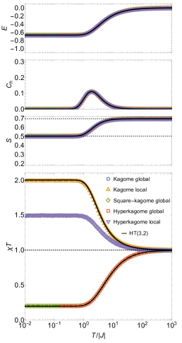
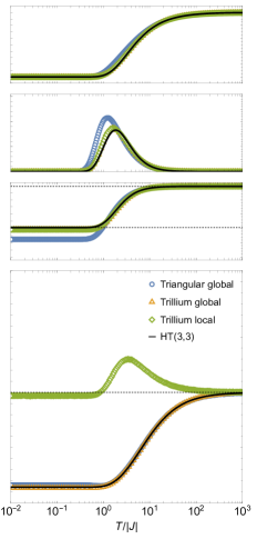
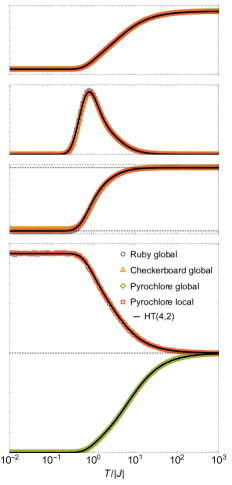
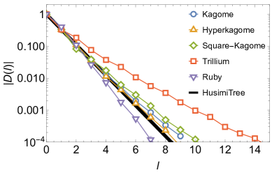
Fig. 5 displays thermodynamic observables: normalized energy , specific heat , entropy and reduced susceptibility , obtained by simulating the Hamiltonian [Eq. (5)] with classical Monte Carlo simulations for the physical lattices [Fig. 2] and analytical calculations on their corresponding Husimi trees [Fig. 3]. As explained in the introduction, these systems have often been studied in the literature; see e.g. Refs. Stephenson (1964); Rastelli et al. (1977); Isoda (2008); Macdonald et al. (2011); Pohle et al. (2016); Jurčišinová and Jurčišin (2018); Richter et al. (2022); Henley (2010); Rehn et al. (2017); Redpath and Hopkinson (2010); Hopkinson et al. (2007); Isakov et al. (2004a); Jaubert et al. (2013); Bovo et al. (2013, 2018); Wills et al. (2002); Kanô and Naya (1953); Wannier (1950, 1973); Pauling (1935); Lieb (1967); Nagle (1966). Our interest here is not to study them individually, but to see how their thermodynamic properties compare to each other. In particular, classical spin liquids are known for their residual entropy as , that measures the degeneracy of the spin-liquid ground state. It can be categorized into three groups Wills et al. (2002); Kanô and Naya (1953); Wannier (1950, 1973); Pauling (1935); Lieb (1967); Nagle (1966) (corresponding to the three columns in Fig. 5), (i) kagome, square-kagome and hyperkagome lattices with , (ii) triangular and trillium lattice with , and (iii) ruby, checkerboard and pyrochlore lattices with . The HT estimate of the residual entropy is also known as Pauling entropy, which, as a side-note, is not always a lower bound [see Appendix C.5].
The behavior of the entropy is accompanied by a change in magnetic correlations from a high-temperature regime with to a model-dependent value at low temperatures [see also Table 1]. The low-temperature Curie constant is not universal, making its value a characteristic property of the underlying spin liquid.
In some models, the value of is easy to understand.
For the ruby, checkerboard and pyrochlore lattice with global axis spins, is zero [Fig. 5 (c)].
This is because their ground state respects the so-called ice rules Bramwell and Harris (1998); Moessner and Chalker (1998a) with two up spins
and two down spins per frustrated cell.
The magnetization is thus not only globally zero on average, , but
also locally zero for all frustrated units.
No fluctuations of the magnetization are allowed in the spin liquid, resulting in and thus a vanishing
reduced susceptibility.
In other words, we get as can be expected for any system with a zero-magnetization plateau.
For triangular frustrated units, the opposite reasoning applies because the magnetization cannot be canceled with three
collinear Ising spins.
Magnetic fluctuations persist down to zero temperature, and and remain finite.
Remarkably, thermodynamic observables match well within each group of lattices, despite their different physical dimensions. It was already knownWills et al. (2002); Kanô and Naya (1953); Wannier (1950, 1973); Pauling (1935); Lieb (1967); Nagle (1966) that some models had very similar residual entropies as . Here this similarity is further illustrated with the value of the spin-liquid Curie law [see Table 1]. But more importantly, thermodynamic quantities are essentially the same for all temperatures within each group of models. For example, the 2D square-kagome model compares well with the 2D kagome, as recently noticed for quantum spins [Richter et al., 2022], but also the 3D hyperkagome, while the 2D ruby model matches with 3D pyrochlore for all temperatures. Furthermore, thermodynamic observables for each group are well reproduced by their corresponding HT, suggesting that correlations barely depend on the physical dimension of the lattice. In the following we will try to understand why.
IV.2 Husimi tree sets the correlation length
As seen in Eq. (10), corresponds to the integration of real-space correlations in the spin liquid [see also Table 1]. Let us consider HT(3,2) whose . This value deviates from Monte-Carlo results on the kagome and hyperkagome lattice within less than 1 %. For the square-kagome lattice, the mismatch drops from 2% to 0.1% by including a more evolved version of the Husimi tree (see HTS in Fig. 3(b)), which contains a larger frustrated unit cell and includes internal loop lengths of four sites. Such a trend suggests the presence of a particularly small correlation length in these systems.
To confirm our suggestion, let us define spin-spin correlations on the HT:
| (11) |
assuming that all spins are collinear along a global axis . The fact that (i) there is no closed loop in the HT (beyond the size of the frustrated unit), (ii) the Hamiltonian is invariant under time-reversal symmetry, and (iii) the HT is by definition locally the same at each vertex, allows us to formulate an exact expression for the spin-spin correlations
| (12) | |||||
The nearest-neighbor spin-spin correlation averaged over the ensemble of ground states can be easily calculated. And it turns out to be the same result for the three kinds of Husimi trees, HT(3,2), HT(3,3) and HT(4,2):
| (13) |
This means that correlations decay exponentially on Husimi trees, following the formula
| (14) |
for all Husimi trees considered here, giving a correlation length
| (15) |
More generally, for a Husimi tree whose frustrated units are made of Ising spins fully connected between each other via antiferromagnetic couplings, the correlation length in the degenerate ground state is
| if is odd, | (16) | ||||
| if is even. | (17) |
Eq. (15) means that correlations decay typically over the nearest-neighbor distance in Husimi trees. This length scale is smaller than any loop in the real lattice, suggesting that correlations in real lattices may decay in a similar way at short distances. Monte Carlo simulations confirm this assumption on the kagome, hyperkagome Hopkinson et al. (2007), square-kagome Pohle et al. (2016) and ruby Rehn et al. (2017) lattice at low temperatures [Fig. 6(a)], whose correlation lengths are roughly the same as . Since the correlation length is expected to decrease upon heating, this short correlation length is consistent with the success of the HT approximation over the whole temperature range for global- and local-axis models alike.
For the sake of clarity, we should point out that the value of is not coming from a cutoff of the correlations beyond . Indeed, it would be tempting to see classical spin liquids as an ensemble of independent clusters of superspins (on each triangle or tetrahedron), and the spin-liquid Curie law as a form of superparamagnetism, as observed with ferromagnetic nanoparticles Néel (1947). However, we cannot recover the value for kagome-type systems from such an argument. Appendix C.4 shows that the resulting error scales like on a Husimi tree of layers. Even if correlations ultimately vanish at long distance, the cutoff necessary to approximately recover the value of is much larger than . To understand the similarity between simulations and analytics, it would be more accurate to see the paths connecting the central spin to the many spins on layer on the infinite-dimensional Husimi tree of Fig. 3 as virtual paths of correlations connecting a pair of nearest neighbors on the corresponding real lattice of Fig. 2. This picture is nearly exact up to the nearest neighbor before closing the minimal loop of size on the real lattice (), which is why deviations between Monte Carlo and Husimi tree grow inversely with in Fig. 6: first hyperkagome, then kagome and finally square-kagome.
IV.3 Coulomb field theory and flat bands
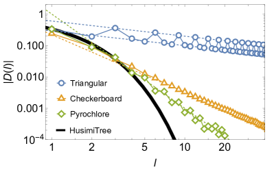
On the other hand, correlations on the checkerboard and pyrochlore lattices are algebraic at low temperature, scaling like [Isakov et al., 2004b], with the physical dimension of the lattice. Their angular dependence is dipolar though, which means that the integration of these correlations over the entire system in Eq. (10) does not diverge, and is well defined. The dipolar nature of these correlations comes from the fact that their ground states are ice models, described by an emergent Coulomb field theory Henley (2010). With respect to the exponential decay of the HT, these algebraic correlations only differ beyond the third or fourth neighbour; see the comparison to the black curve on Fig. 6(b). In that sense the correlation length remains effectively relevant at short distances. That being said, one would have been forgiven to expect larger corrections to coming from the long-range algebraic tail. Here again we are left with the question: why are these corrections so small ?
For models with a global axis, is known to be exactly zero (see discussion in Section IV.1); the ice rules prevent magnetic fluctuations for all tetrahedra, and thus conveniently prevent any corrections. But this does not explain the match of Fig. 5(c) for the local-axis pyrochlore model, a.k.a. spin ice, where . Magnetic fluctuations are allowed in the spin-ice ground state. Additionally, since the spin-ice model is ferromagnetic, the sum of Eq. (8) contains mostly positive terms, as opposed to the alternating series encountered for the integration of correlations in antiferromagnets [Appendix C.4]. For the latter, potential corrections coming from algebraic correlations would partially cancel out; while they would a priori add up in the ferromagnetic model. This suggests that an alternative point of view is necessary.


Let us temporarily step away from Husimi trees and consider the other facet of spin ice, as a U(1) Coulomb gauge field. As mentioned previously this gauge-field texture comes from the ice rules, that can be rewritten as a divergence-free constraint on the magnetisation field [Henley, 2010]. But spin ice is not the only model supporting this type of texture. The ground state of the pyrochlore antiferromagnet with classical Heisenberg spins is a U(1)U(1)U(1) Coulomb gauge field that has often been described as three copies of spin ice Canals and Garanin (2001, 2002); Isakov et al. (2004b); Henley (2010). The susceptibility of these divergence-free fields is readily available using the Self-Consistent Gaussian Approximation (SCGA). It means that with the proper normalisation, SCGA offers an alternative approach to compute and [see Appendix D]. In particular it tells us that the ratio is due to the topology of the magnetic band structure of the pyrochlore lattice Reimers et al. (1991); Conlon and Chalker (2010); Conlon (2010); Benton (2014); the ground state is composed of two degenerate flat bands, accounting for half () of the total number of bands.
To summarise, since comes from the integration of correlations [Eq. (10)], it is remarkable that algebraic correlations in real lattices give almost the same result as exponential correlations in Husimi trees [see pyrochlore and checkerboard results in Fig. 5]. This is because is protected by the absence of local fluctuations for global-axis models, while is a direct consequence of the topology of the band structure for local-axis models.
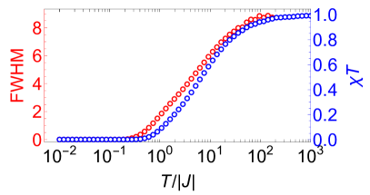
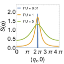
Before closing our discussion on the checkerboard and pyrochlore lattices, let us take advantage of these dipolar correlations, whose signatures in the equal-time structure factor present sharp, singular features known as pinch points Youngblood and Axe (1981); Harris et al. (1997); Henley (2010). Upon heating, these singular features broaden as topological-charge excitations disrupt the Coulomb field [Fig. 7 (a)–(c)] Fennell et al. (2009). By measuring their breadth, pinch points offer a quantitative way to measure the establishment of the spin liquid. Fig. 7(d) shows the full width at half maximum (FWHM) of the pinch point on the checkerboard lattice as a function of temperature. Our point is that the Curie-law crossover, as seen in , is able to grasp the evolution of FWHM, i.e. the build up of the spin liquid. And while only a fraction of spin liquids have characteristic, singular, patterns such as pinch points, the Curie-law crossover is a generic property of all spin liquids. This vindicates the Curie-law crossover as a useful signature of the onset of a spin liquid, and the reduced susceptibility as a suitable observable to measure it.
IV.4 The triangular and trillium lattice
Let us now consider two systems with noticeably different geometries; the triangular and trillium lattice. While the latter is three dimensional and made of corner-sharing triangles, the former is two dimensional and usually seen as made of edge-sharing triangles. From the view point of Husimi trees, HT(3,3) is clearly a reasonable approximation for the trillium lattice, with each spin belonging to three triangles. But, even if less conventional, it can also be used for the triangular lattice Monroe (1998b); Jurčišinová et al. (2014b), since each spin can similarly be seen as shared by three triangles (see colored lattice in Fig. 2(a)). The obvious caveat of this choice of Husimi tree (made of 3 spins) is that loops that are ignored, are of the same size than the frustrated triangular unit cell itself. However, by direct comparison between MC and HT(3,3) results in Fig. 5(b), the reduced susceptibility, , of the two antiferromagnetic models overlap with a quantitative difference appearing only below [Fig. 8].
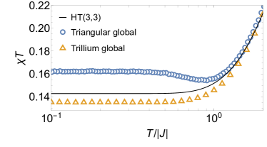
The excellent match above is in part due to the fact that the nearest-neighbour correlations in the degenerate ground state is [Stephenson, 1964], for triangular and trillium systems in accordance with their corresponding Husimi tree [see Eq. (13)]. Indeed, the ground state energy is , where is the number of nearest-neighbour bonds. For , correlations beyond nearest neighbours apparently start to play a role on the real lattices. From Fig. 8, the deviation from the HT curve indicates a dominant antiferromagnetic (resp. ferromagnetic) contribution for the trillium (resp. triangular) lattice [Eq. (8)]. In the triangular case, the third nearest-neighbour correlations are known to be strongly ferromagnetic Stephenson (1964); Rastelli et al. (1977), with , as . It is likely that this increase of ferromagnetic correlations in the ground state causes an upturn of the reduced susceptibility [Fig. 8]. Accordingly, integrated correlations in the triangular Ising antiferromagnet are more antiferromagnetic at finite temperature, for , than in the spin-liquid ground state. Such a non-monotonic behavior of the reduced susceptibility is unusual, but not rare.
It is even more pronounced for the trillium lattice with easy axes. The reduced susceptibility of easy-axes models necessarily increase upon cooling from high temperature, because nearest neighbor correlations are always ferromagnetic (the scalar product in Eq. (6) is always negative). For the trillium lattice, however, one can show that [see Appendix C.4.7]. It means that has to decrease at low temperature.
V Husimi Ansatz for the Curie-law crossover
V.1 Limitation of the Curie-Weiss fit
As mentioned in the introduction, the Curie-Weiss temperature is a mean-field estimate of the transition temperature for a system with connectivity , where the Curie-Weiss law is a consequence of critical scaling invariance with critical exponent . Even though the concept of conventional order does not apply to spin liquids, does represent a meaningful quantity, as a measure of interaction strength. The practical question is, how accurately can this quantity be measured in experiments ?
Best estimates can only be made at high temperatures, since is the first-order correction to the Curie law
| (18) |
And here is the main issue with the Curie-Weiss temperature . In magnets, the high-temperature regime is frequently not accessible, since it is two or three orders of magnitude larger than the characteristic exchange coupling . For example in magnets with valence electrons, is often of the order of K and the high-temperature regime is inaccessible because it lies above the melting point of the crystal. On the other hand for magnets with valence electrons, is much smaller, of the order of K. But ions have a large single-ion degeneracy, lifted by the local crystal field. This crystal field introduces a single-ion anisotropy with an associated energy scale, which varies a lot from one material to another, but the lowest single-ion excitation is usually of the order of K. The high-temperature region is thus difficult to access because the nature of magnetic moments changes with temperature Li et al. (2021). We refer the reader to the useful tutorial written by Mugiraneza & Hallas [Mugiraneza and Hallas, 2022] for a practical, step-by-step, application of the Curie-Weiss fit.
The susceptibility measures the evolution of the spin-spin correlations [Eq. (8)]. And the problem is that, as we have seen throughout this paper, this evolution from paramagnetism to spin liquid takes place over several orders of magnitude in temperatures. It is thus naturally best seen on a logarithmic scale. Applying the Curie-Weiss law, which is a linear fit, can be dangerous. What appears to be a reasonable temperature window on a linear scale might actually only measure a small evolution of the spin-spin correlations. The Curie-Weiss fit will always give a result of course, but the outcome will depend on the window of measurement [Fig. 1]. And if the high-temperature regime is not available, then it is not possible to check if the value is correct or not, causing a potentially (largely) inaccurate estimate of .

V.2 The Husimi Ansatz
To measure the Curie-Weiss temperature in spin liquids, a complementary approach, relying on data points within an experimentally accessible temperature region, would be welcome.
While very high-temperatures are often physically not accessible, very low-temperatures are also not ideal. Irrespectively of the possible difficulty to thermalise the sample, perturbations beyond the spin-liquid Hamiltonian usually set a temperature scale below which the physics of the spin liquid is lost; the system may order or fall out-of-equilibrium. The most appropriate window in experiments is thus at intermediate temperatures, precisely where the crossover between the two Curie laws takes place. And while low- and high-temperature expansions are the least accurate in this regime, Section IV.1 has shown that HT calculations are quantitatively reliable over the entire temperature region for corner-sharing lattices.
Appendix C.2 gives the analytical formula of the susceptibility for different geometries of the Husimi tree. We notice that the reduced susceptibility is always of the form
| (19) |
This expression is sufficiently generic that it should be able to fit any form of . But as it is written, Eq. (19) is unpractical. Fortunately, it turns out that only a few terms are usually necessary. The simplest pertinent form of Eq. (19) is
| (20) |
We shall refer to Eq. (20) as the Husimi Ansatz. In this form the Curie constant and Curie-Weiss temperature can be directly extracted from the fitting parameters:
| (21) | ||||
| (22) |
Eq. (20) will be our primary phenomenological Ansatz for the rest of this paper. Intuitively, we understand that the and parameters correspond to effective energy scales in the Boltzmann factor. However, two energy scales might be too minimal to describe the physics of some models, especially if different types of couplings are involved. This is why we will also consider an extended Ansatz to fit
| (23) |
where the Curie constant and Curie-Weiss temperature become
| (24) | ||||
| (25) |
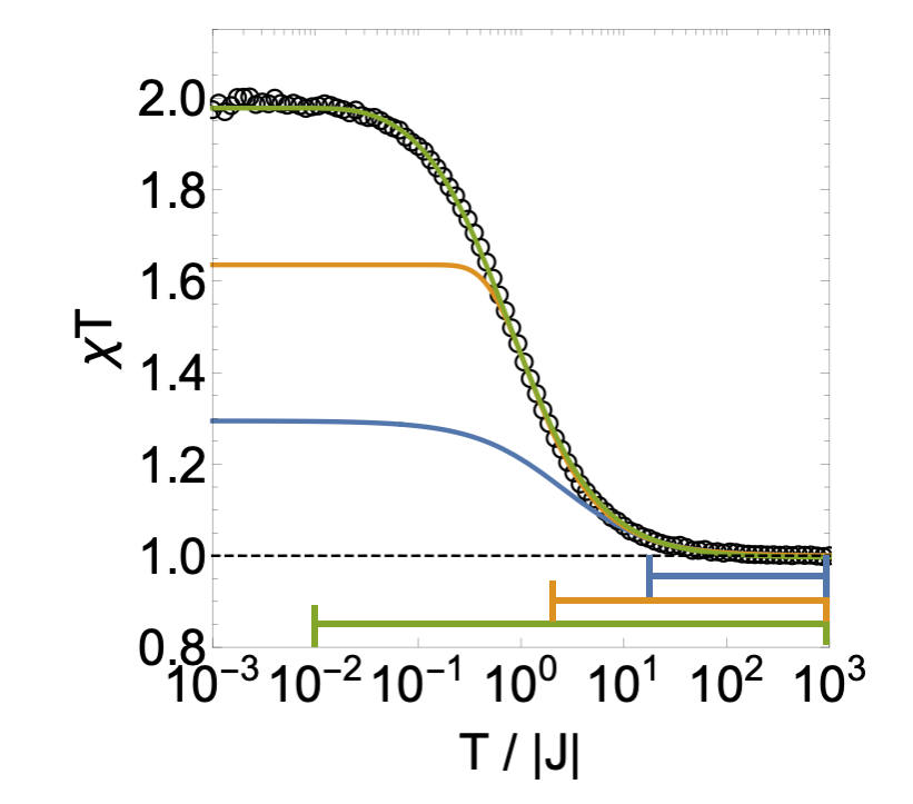
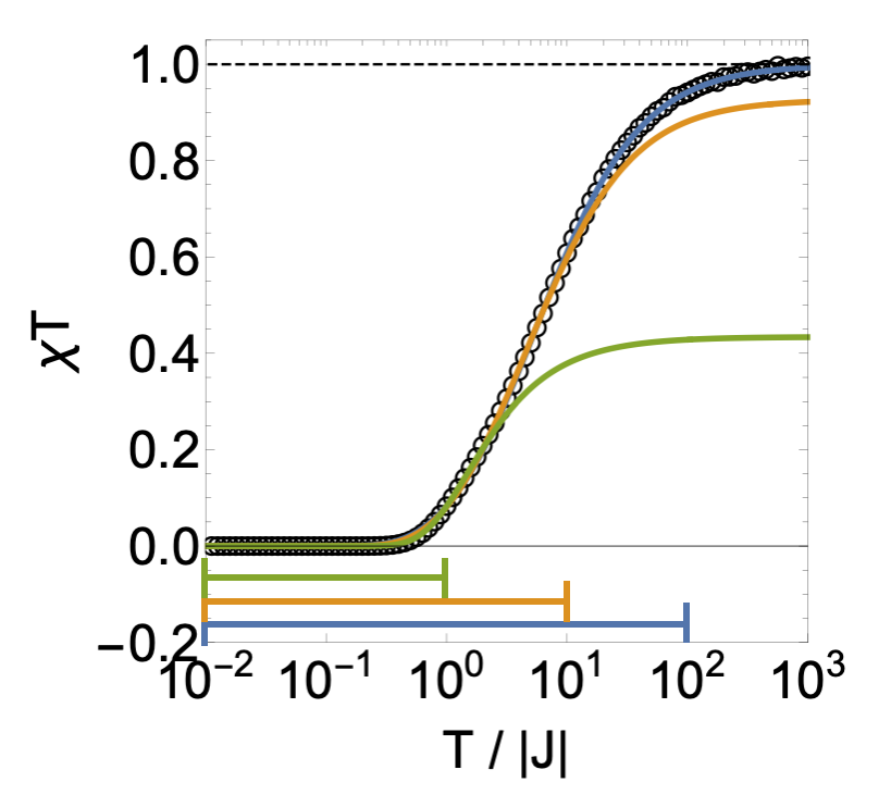
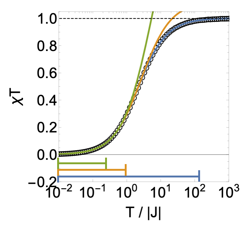
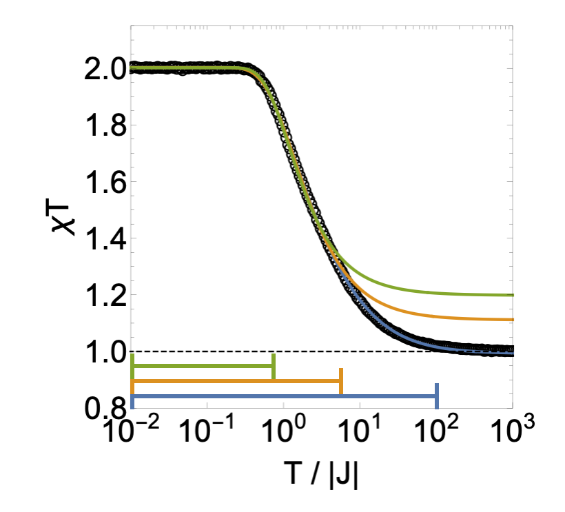
V.3 Benchmark of the Husimi Ansatz
The purpose of this section is to benchmark the Husimi Ansatz of Eq. (20) in a controlled way on various model Hamiltonians. In Fig. 9 we fit the Curie-law crossover with Eq. (20) for pyrochlore models with global-axis and local-axis Ising spins. In order to test the Ansatz on a general framework, beyond the Ising models used to build our Husimi-based intuition, we also consider continuous spins on the Heisenberg antiferromagnet (HAF) Moessner and Chalker (1998b); Canals and Garanin (2001); Henley (2005), and pseudo-Heisenberg antiferromagnet (pHAF) Ross et al. (2011); Onoda and Tanaka (2011); Lee et al. (2012); Taillefumier et al. (2017). The pHAF is defined on the XXZ model as follows:
| (26) |
with along the local [111] easy-axis, as defined in Tab. 4, for parameters Taillefumier et al. (2017). This model is thermodynamically equivalent to the HAF, but with different magnetic correlations, and thus a distinct evolution of the Curie-law crossover.
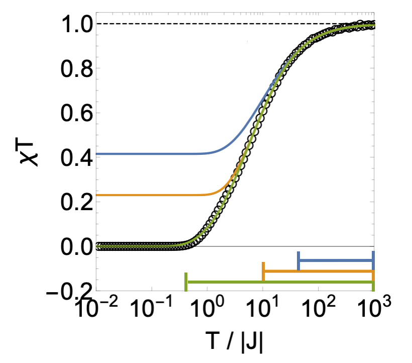
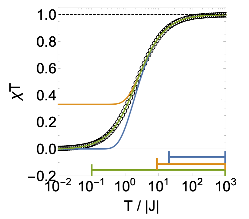
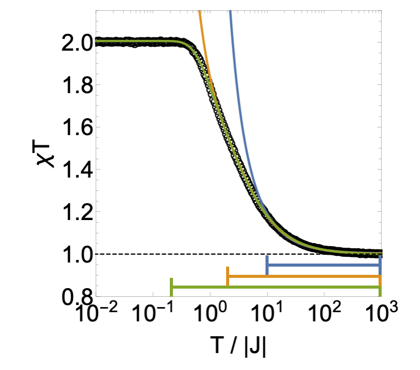
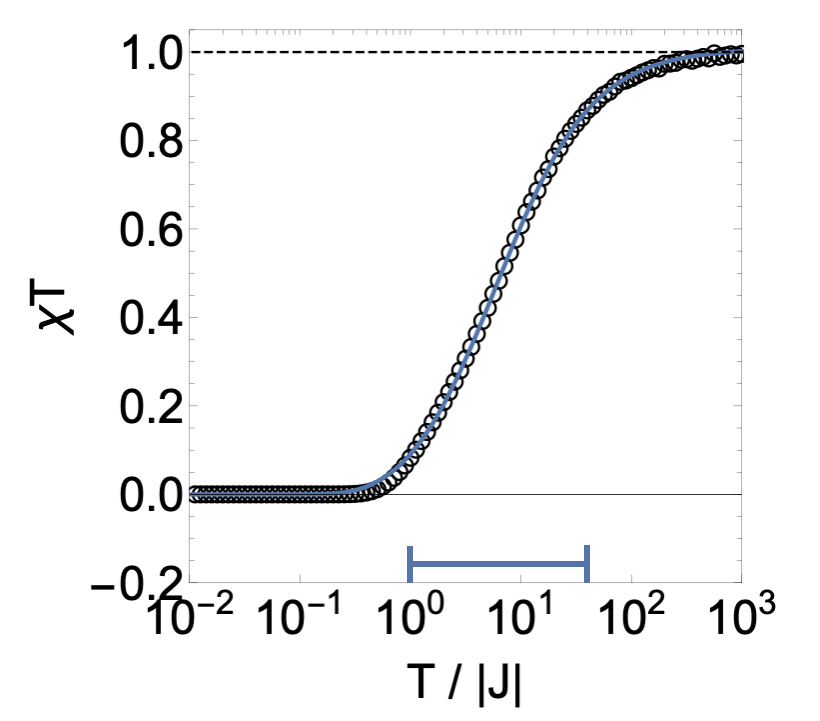
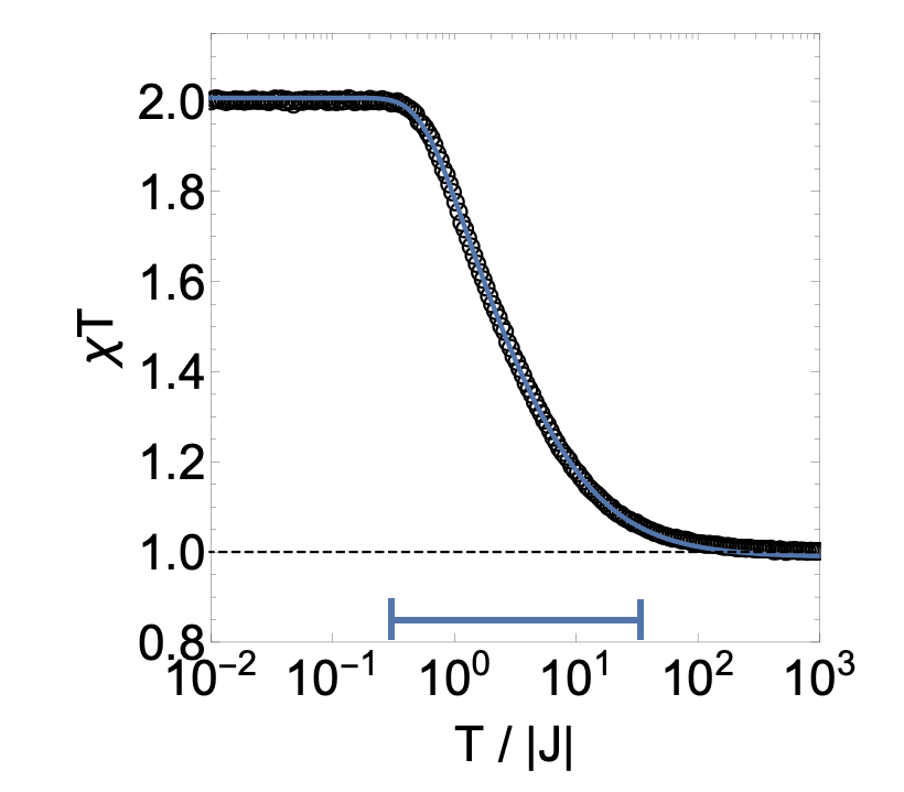
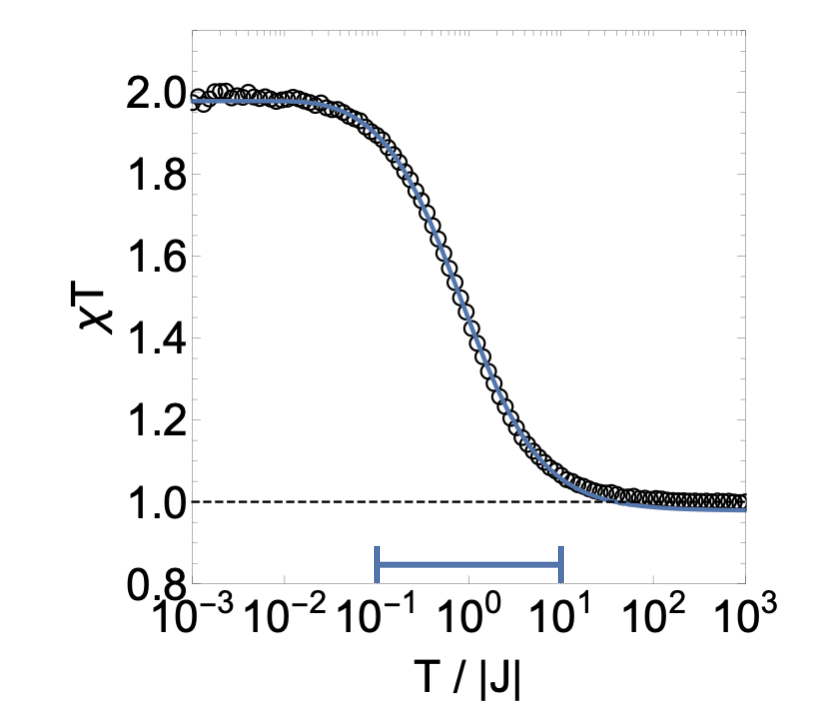
Fig. 9(a) and (b) show vanishing , induced by the zero-divergence constraint on the ground state manifold, imposing zero magnetisation in all tetrahedra (see discussion in Section IV.1). Fig. 9(c) and (d) show , as a result of dominant ferromagnetic correlations. Entering the spin-liquid regime at low for (a) and (c) for models with Ising degrees of freedom shows a rather sharp kink below , while on the opposite, models with continuous degrees of freedom in (b) and (d) enter the low regime rather smoothly.
Results were obtained from classical MC simulations (black circles) and have been fitted with the Husimi Ansatz (solid lines) from Eq. (20) over different temperature windows. Examples of three different fitting windows are shown for high-temperature (1st row), and low-temperature (2nd row) fits. The range of fitting windows are indicated by blue, yellow and green bars on the bottom of each plot, and allow to judge their reliability in comparison to MC data. It becomes clear that fitting windows, which include only one Curie-law regime (either at low or high temperature), do not accurately reproduce the Curie-law crossover. This is especially important for Ising models, because of the relatively sharp kink when entering the spin-liquid regime.
On the other hand, fitting windows including the intermediate temperature window, with only the onset of high- and low-temperature regimes quantitatively reproduce over the full temperature range. The 3rd row of panels shows the “minimal” fitting window. By using Eqs. (21, 22) we can precisely extract the Curie constant and Curie-Weiss temperature from those fits. Fitted and exact solutions match perfectly within error bars (see Tab. 2).
| model | ||||
| fit | exact | fit | exact | |
| Ising global | ||||
| HAF | ||||
| Ising local | ||||
| pHAF | 2/3 | |||
This benchmark shows that the Husimi Ansatz correctly reproduces the Curie-law crossover over the full range of temperatures for several distinct models with Ising and continuous spins. It requires a fitting window spanning typically 1 or 2 orders of magnitude in temperature, in the intermediate regime that is usually accessible to experiments [see the bottom row of Fig. 9]. This is a useful theoretical proof of concept, that now needs to be applied to experiments.
VI The Husimi Ansatz in experiments
Our goal in this section is to show by examples the advantages and limitations of the Husimi Ansatz in real materials, and to encourage its use jointly with the Curie-Weiss fit.
VI.1 NaCaNi2F7
First, let us consider a material where the Ansatz gives similar results to the Curie-Weiss fit. To do so, let us consider one of the closest materials to the canonical HAF.
NaCaNi2F7 is a spin pyrochlore material, well described by a weakly perturbed nearest-neighbour Heisenberg Hamiltonian Plumb et al. (2019); Zhang et al. (2019). It shows spin freezing at , which has been assumed to originate from Na1+/Ca2+ charge disorder, however, no long-range magnetic order has been observed Krizan and Cava (2015).
In Fig. 10, we plot the magnetic susceptibility of NaCaNi2F7, extracted from Ref. [Krizan and Cava, 2015], on a semi-logarithmic scale for and on a linear scale for . The data points are well fitted by the Husimi Ansatz of Eq. (20) over the whole range of accessible temperatures.
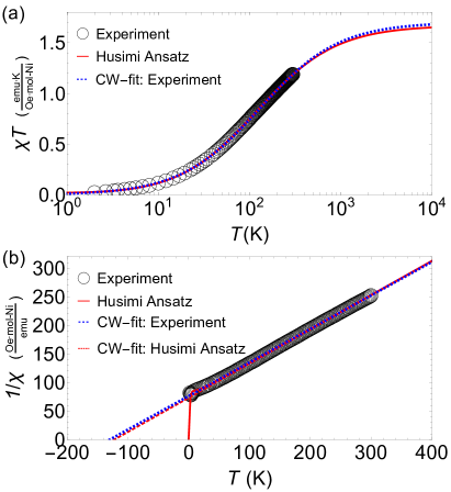
We fit the Husimi Ansatz within physically relevant temperatures , above the freezing transition up to the maximally available datapoints, and obtain a Curie-Weiss temperature , and a Curie constant (emu K)/(Oe mol-Ni), which gives an effective magnetic moment of . All these quantities are in good agreement with a standard Curie-Weiss fit over a temperature window , which reveals with . This strongly suggest, as also qualitatively visible from the straight behavior of in Fig. 10(b), that experimentally measured data points reach the high-temperature regime where a standard Curie Weiss fit becomes a reliable estimate.
VI.2 KCu6AlBiO4(SO4)5Cl
KCu6AlBiO4(SO4)5Cl is a promising quantum spin liquid candidate on the distorted square-kagome lattice, as reported by M. Fujihala et al. in Ref. [Fujihala et al., 2020]. Measurement of specific heat and susceptibility did not find any signatures of long-range order down to , while SR confirmed the absence of spin order and spin freezing down to .
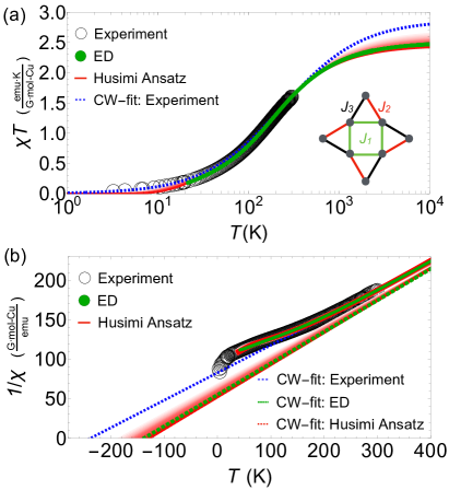
In Fig. 11, we plot the magnetic susceptibility of KCu6AlBiO4(SO4)5Cl, as kindly provided by M. Fujihala [Fujihala et al., 2020], on a semi-logarithmic scale for and on a linear scale for . In comparison to NaCaNi2F7 in Fig. 10(b), it becomes evident that for KCu6AlBiO4(SO4)5Cl shows a rather strong deviation from a linear behavior over nearly the whole range of experimentally accessible temperatures. A Curie-Weiss fit for the high-temperature tail within gives and with a Landé factor Fujihala et al. (2020). The Husimi Ansatz from Eq. (20) gives a noticeably different outcome though. We find . The large error bar comes from the choice of the fitting temperature window [] (see the spread of the red curve in Fig. 11), where we fix at the highest available temperature, and vary between and . The non-linearity of and spread of the Husimi estimate suggest that is too far from the high-temperature limit for a conclusive estimate of . The noticeable difference between the outcomes of the Curie-Weiss fit and Husimi Ansatz, however, makes us wonder which of the two estimates is more reliable.
From a microscopic analysis in [Fujihala et al., 2020] we understand that KCu6AlBiO4(SO4)5Cl is not an ideal square-kagome lattice; the three bonds of a triangle in Fig. 2(c) are inequivalent. All triangles are distorted in the same way and form three distinct “nearest-neighbour” couplings, , on each triangle (see inset in Fig. 11.(a)). M. Fujihala et al. Fujihala et al. (2020) built a microscopic Hamiltonian which describes its magnetic susceptibility at high temperature, using exact diagonalization (ED) and finite-temperature Lanczos methods, as shown on Fig. 11. ED results fit the experimental data very well down to , below which finite-size effects make further estimates difficult. M. Fujihala et al. obtained
| (27) |
with a Landé factor . This high-temperature analysis cannot rule out low-energy perturbations, but it establishes the model of M. Fujihala et al as a solid parametrisation of KCu6AlBiO4(SO4)5Cl in the temperature regime relevant to , which is straightforward to estimate from Eq. (27)
| (28) | |||||
| (29) |
Eq. (29) leads to a couple of remarks. Firstly, the ED results are in better agreement with the Husimi Ansatz than the Curie-Weiss fit, which a posteriori validates the former. Secondly, here simply corresponds to the average value of the three inequivalent exchange couplings. fit within the energy window set by , thus defining the anisotropic energy scale K. Using as a lower bound of our fitting temperature window, we obtain from the Husimi Ansatz with a Landé factor , which is essentially the same result as from ED111It is worth noting that a Landé factor of 2.1 is a more realistic value for Cu(II) ions than the value of 2.25 found with the Curie-Weiss fit.. This suggests that the main difficulty to estimate comes from the lattice anisotropy of KCu6AlBiO4(SO4)5Cl. And while the Curie-Weiss law is not adapted to account for multiple energy scales in this intermediate regime, the Husimi Ansatz has been designed to be a flexible fitting function for the crossover that happens in this intermediate regime. We believe it is the reason why the Husimi Ansatz, albeit its large error bar, gives a better result than the Curie-Weiss fit.
VI.3 FeCl3
VI.3.1 Experiments
As seen from the two previous materials with negative Curie-Weiss temperatures, spin liquids usually show dominant antiferromagnetic couplings. However, there also exist frustrated magnets where the interplay between ferro- and antiferro-magnetism can lead to multiple Curie-law crossovers Pohle et al. (2016); Schmidt and Thalmeier (2017). An important example relevant to materials are spiral spin liquids. They form a class of classical spin liquids where spiral states compete and form a sub-extensive ground state manifold with characteristic ring features in momentum space Niggemann et al. (2019); Pohle et al. (2021); Yao et al. (2021); Huang et al. (2022); Yan and Reuther (2022).
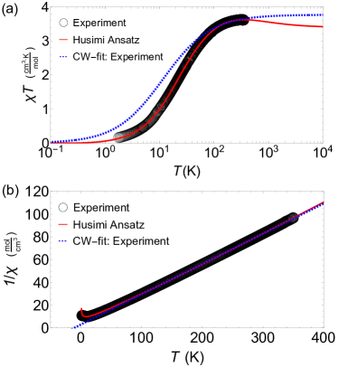
The Van der Waals magnet FeCl3 is a prototype of a spiral spin liquid. At first, investigated as a member of crystallized anhydrous ferric chlorides Lallemand, A. (1935), the history of FeCl3 dates far back into the 1930’s, where it already attracted attention due to its unusual magnetic properties at low temperature. Susceptibility measurements reported a Curie-Weiss temperature of , however, noticing already at that time a deviation from the conventional Curie-Weiss law Starr et al. (1940). Furthermore, inelastic neutron-scattering (INS) measurements Cable et al. (1962), magnetic susceptibility Jones et al. (1969), Möessbauer effect Stampfel et al. (1973), magnetic field Johnson et al. (1981), and NMR measurements Kang et al. (2014) confirmed a phase transition into an unusual spiral ground state at about . But it was only recently, with the work of S. Gao et al. [Gao et al., 2022], that continuous ring features around the -point could be observed in INS experiments; a clear evidence of spiral spin liquid physics in FeCl3.
In Fig. 12 we show the magnetic susceptibility of FeCl3, as kindly provided by M. McGuire [Gao et al., 2022], on a semi-logarithmic scale for and on a linear scale for . In contrast to the materials above (see Fig. 10 and Fig. 11), it seems that reaches the plateau of the high-temperature Curie-Weiss regime already at about . For the traditional vs plot [Fig. 12.(b)], the Curie-Weiss law shows a good fit over the temperature window , which gives , in agreement with previous measurements Starr et al. (1940). However, when plotting the reduced susceptibility instead [Fig. 12.(a)], the Curie-Weiss law is seen to noticeably deviate from experimental data below 50 K. In fact, after careful consideration, experimental data show a broad maximum at about , suggesting that the reduced susceptibility is not monotonic. This motivates us to fit the available experimental data with the extended Husimi Ansatz of Eq. (23) which allows for non-monotonic behavior. It fits the experimental data quantitatively well over the whole temperature range and indeed presents a slight downturn at high temperatures above . Unfortunately, FeCl3 is structurally unstable at higher temperatures and there are not enough data points after the downturn of to extract a reliable estimate of . And since susceptibility measurements are naturally more noisy at high temperature, one should remain cautious. That being said, the Husimi Ansatz suggests a positive Curie-Weiss temperature in FeCl3 – as opposed to previous measurements Lallemand, A. (1935); Starr et al. (1940); Jones et al. (1969) – and thus a multi-step Curie-law crossover with dominant ferromagnetic interactions, that would justify the anomalous behavior of the susceptibility that has been noticed since 1940 Starr et al. (1940).
VI.3.2 Simulations
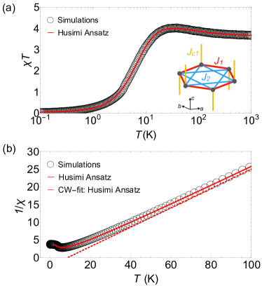
In absence of data points for FeCl3 at high temperature, it is difficult to push the experimental analysis any further. Therefore, to conclude this discussion on the multi-step Curie-law crossover, we shall turn to classical Monte Carlo (MC) simulations. Magnetic Fe3+ () ions cover honeycomb layers, which are stacked in an arrangement along the axis. By comparing LSW theory and SCGA results to INS data, S. Gao et al. [Gao et al., 2022] proposed a series of models with up to nine coupling parameters. For the sake of simplicity, we will focus on their minimal model, which is able to reproduce the ring features of a spiral spin liquid; the -- Heisenberg model (see inset in Fig. 13.(a)).
| (30) |
where
| (31) |
The couplings and respectively account for nearest-neighbor and next nearest-neighbor interactions within individual honeycomb layers, while is the nearest-neighbor antiferromagnetic interlayer coupling.
In Fig. 13 we show the susceptibility, measured from MC simulations of [Eq. (30)]. Now the multistep Curie-law crossover becomes evident, even from simulation data, and the extended Husimi Ansatz from Eq. (23) gives , with a Curie constant . It means that, taken in its extended form, the Husimi Ansatz can also account for a non-monotonic evolution of due to competing ferro- and antiferromagentic couplings.
VI.4 Summary about experimental comparison
In this section, we analyzed magnetic properties for three spin liquid candidates, namely, the pyrochlore fluoride NaCaNi2F7, the square-kagome material KCu6AlBiO4(SO4)5Cl, and the spiral spin liquid on the honeycomb lattice FeCl3. All three materials showed a Curie-law crossover over a wide temperature range, from up to . Considering those examples, it becomes clear that a conventional Curie-Weiss fit applied to spin liquids can be reliable, but does not always have to. Depending on the microscopic model parameters and the nature of the underlying spin liquid, the high-temperature Curie-Weiss regime might not be practically accessible. We showed, that the comparison between the conventional Curie-Weiss fit and the Husimi Ansatz, as introduced in Sec. V.2, allows us to quantify whether the high-temperature regime of a material is reached or not.
NaCaNi2F7 is an example where experiments could reach to the high-temperature regime, and results from Husimi Ansatz and Curie-Weiss fit gave nearly the same results.
On the other hand, KCu6AlBiO4(SO4)5Cl, shows a rather nonlinear behavior of in Fig. 11(b) for the available temperatures in experiment, which results in a mismatch between standard the Curie-Weiss fit and the Husimi Ansatz. The latter, however, agrees with independent ED results.
Last but not least, FeCl3 is probbaly an example of a multi-step Curie-law crossover. Such non-monotonic behavior of magnetic correlations cannot be described by a conventional Curie-Weiss law, and therefore requires extra caution. By comparison to a minimal Heisenberg model we showed that an extended Husimi Ansatz [Eq. (23)] is able to capture such a non-monotonic Curie-law crossover, predicting a Curie-Weiss temperature which is noticeably different compared to the one obtained from a standard Curie-Weiss fit.
In addition, some materials support the physics of a spin liquid at low but finite temperature, before ordering (or spin-freezing) at ultra-low temperatures . The mechanism is simple. Let us consider a pristine spin-liquid model with a Curie-Weiss temperature . By definition, this system doesn’t order. Now, let us add a relevant, but small, perturbation of energy scale inducing a transition at . One expects the spin-liquid physics to persist for a certain temperature window above . But to determine the extent of this window is not easy without a microscopic probe such as neutron scattering, NMR or SR. Fortunately, by plotting the reduced susceptibility on a logarithmic temperature scale, we immediately measure the build-up of magnetic correlations upon cooling [Eq. (10)] and can thus estimate how close we are from the spin-liquid regime. This is the case of NaCaNi2F7 which has a spin-freezing transition at . On Fig. 10.(a), we see that approaches the low-temperature spin-liquid Curie law (with here) at K. It means that NaCaNi2F7 supports the spin-liquid physics of the pyrochlore antiferromagnet over the temperature window . It also means that the Husimi Ansatz can be used successfully even if the system orders at ultra-low temperature.
VII Conclusions
The Curie-Weiss temperature is a useful quantity to estimate the strength of frustration in frustrated magnets [Eq. (2)]. However, the Curie-Weiss law is an estimate of the magnetic susceptibility close to a mean-field critical point, which – by definition – is absent in frustrated magnets. In this Article, we have shown that the concept of a Curie-law crossover Jaubert et al. (2013) is a generic feature for spin liquids and a more accurate description of their thermodynamic properties, that can be used to partially classify them. We systematically study the Curie-law crossover among a variety of frustrated Ising models in two and three dimensions [Fig. 2], and motivate its relevance to thermodynamic signatures, as seen in experiments. Comparing unbiased Monte Carlo simulations with the analytical Husimi-Tree approximation shows that the Curie-law crossover is determined by the type of frustrated unit cell (triangle, tetrahedron, …) and the connectivity between them, rather than the physical dimension of the lattice. As a side note, the Husimi-Tree approximation proves to be quantitatively accurate for all temperatures and for many spin-liquid models [Fig. 5].
As a consequence of the Curie-law crossover, we recommend using the reduced susceptibility , complementary to the usual plot, when studying a potential spin liquid. It is often difficult to estimate whether has reached the asymptotic linear behavior, while quickly indicates how far we are from the high-temperature Curie law.
Based on the success of the Husimi-Tree approximation, we propose an empirical Ansatz [Eq. (3)] as a useful complement to the Curie-Weiss law. The Husimi Ansatz is easy to use and designed to be a flexible fitting function for the crossover in that takes place in the temperature regime which is typically accessible to experiments. This means that the Husimi Ansatz can be used on a broader temperature window than the Curie-Weiss fit, which is necessarily limited to the region where is linear in . In its extended form [Eq. (23)], the Husimi Ansatz can also take into account the competition between ferro- and antiferromagnetic couplings in multi-step Curie-law crossovers.
It should be noted that the approach developed here works for frustrated magnets in general. Frustration doesn’t need to be geometric in origin, it may come from further neighbor or anisotropic spin exchange, as present in Kitaev materials. And even if the simulations and calculations were based on classical spins in this paper, the Husimi Ansatz can be applied to quantum materials in the crossover regime, as done in Section VI.
Acknowledgements.
The authors thank Harald Jeschke, Elsa Lhotel, Rodolphe Clérac, Claire Lhuillier, Nic Shannon, Benjamin Canals for fruitful discussions, and Shang Gao, Jason Krizan and Yukitoshi Motome for critically reading the manuscript. This work was supported by the Theory of Quantum Matter Unit, OIST and “Quantum Liquid Crystals” JSPS KAKENHI Grant No. JP19H05825. L.D.C.J. acknowledges financial support from CNRS (PICS France-Japan MEFLS) and from the French ”Agence Nationale de la Recherche” under Grant No. ANR-18-CE30-0011-01. Numerical calculations were carried out using HPC Facilities provided by OIST, and the Supercomputer Center of the Institute for Solid State Physics, the University of Tokyo.Appendix A Definition of local easy axes
We provide positions and definitions for the local easy axes of Ising spins [see Eq. (6)] for the kagome (Tab. 3), pyrochlore (Tab. 4), hyperkagome (Tab. 5) and trillium lattice (Tab. 6). Models with global and local axes are equivalent up to a rescaling in the exchange coupling given in each table caption.
| site index | position | |
| 1 | ||
| 2 | ||
| 3 |
| site index | position | |
| 1 | ||
| 2 | ||
| 3 | ||
| 4 | ||
| 5 | ||
| 6 | ||
| 7 | ||
| 8 | ||
| 9 | ||
| 10 | ||
| 11 | ||
| 12 | ||
| 13 | ||
| 14 | ||
| 15 | ||
| 16 |
| site index | position | |
| 1 | ||
| 2 | ||
| 3 | ||
| 4 | ||
| 5 | ||
| 6 | ||
| 7 | ||
| 8 | ||
| 9 | ||
| 10 | ||
| 11 | ||
| 12 |
| site index | position | |
| 1 | ||
| 2 | ||
| 3 | ||
| 4 |
Appendix B Monte Carlo simulations
Numerical Monte Carlo (MC) simulations of the Hamiltonian [Eq. (5)] for Ising spins (Ising model) were performed by updating the site dependent Ising variable for systems larger than spins. To account for statistically independent samples at very low temperatures a local single-spin flip Metropolis update algorithm has been used in combination with parallel tempering Swendsen and Wang (1986); Earl and Deem (2005), and a worm-update algorithm Barkema and Newman (1998); Prokof’ev and Svistunov (2001) in the case of the checkerboard, pyrochlore and ruby lattice. A single MC step consists of local single spin-flip updates on randomly chosen sites, and 5 worm updates (checkerboard, pyrochlore and ruby lattice), performed in parallel for replicas at 100 to 200 different temperatures, with replica-exchange initiated by the parallel tempering algorithm every MC step.
MC simulations of the Hamiltonian [Eq. (5)] for Heisenberg spins (Heisenberg model) were performed by using a local heat-bath algorithm Olive et al. (1986); Miyatake et al. (1986), in combination with parallel tempering Swendsen and Wang (1986); Earl and Deem (2005), and over-relaxation Creutz (1987). Here, a single MC step consists of local heat-bath updates on randomly chosen sites, with over-relaxation steps, flipping the spin direction about their local exchange field, and replica-exchange every MC step.
In both cases, simulations for Ising and Heisenberg models, thermodynamic quantities were averaged over statistically independent samples, after MC steps for simulated annealing and MC steps for thermalization.
Appendix C Husimi Tree
C.1 Explicit calculations for the kagome Ising antiferromagnet
In this section, the Husimi tree calculation shall be explained on the example of HT(3,2) [see Figs.3(a) and 14(a)]. Branches of nonintersecting triangular cells spread out from the central unit (shell 0, drawn in red). Let us consider the Hamiltonian Eq. (5) for Ising spins on sites with an additional external magnetic field
| (32) |
At the end of the calculations, the magnetic field will be taken vanishingly small in order to obtain the susceptibility . The magnetisation on one of the central site (chosen arbitrarily) is
| (33) | ||||
| (34) |
being the total partition function. denotes the product over all nearest-neighbour pairs within the central triangular plaquette. is the partition function of the branch of the Husimi tree moving outwards and starting from the central spin with orientation .
Let us label the partition function starting on site belonging to the layer of the tree. The Boltzmann weights are
| (35) | ||||
| (36) |
taking the values , and here [Fig. 14(b)]. Eq. (33) then gives explicitly
| (37) |
where we introduced the ratio between partition functions of a spin on shell , pointing () and a spin pointing down ( Baxter (1982) as
| (38) |
and where successive layers of the Husimi tree are related recursively
| (39) |
To solve the Husimi tree, we calculate the limit and replace it in Eq. (37), 222Please note that we use this numbering of layers – increasing outwards – essentially for pedagogical reasons. Mathematically, the problem is well posed if we consider a change of variable: layer 0 would be on the outer boundary, infinitely far away from the central layer which would be labeled . Following this notation, this is why the limit can be used in Eq. (37).. In absence of an external magnetic field , since the disordered system does not prefer any spin direction. This gives as trivially expected. But other observables such as the energy , specific heat and entropy can be derived analytically from the partition function . These calculations are relatively straightforward and explicit results for the different Husimi trees are given in Appendix C.2.
In this section, we will further show the calculation of the susceptibility. An external magnetic field causes a perturbation away from the trivial value
| (40) |
which can be used together with Eqs. (38),(39) to obtain in first order of
| (41) |
The first-order expansion in is sufficient to compute the magnetic susceptibility, since higher-order terms vanish as . Introducing Eqs. (38)–(41) into Eq. (37) gives the temperature-dependent magnetisation
| (42) |
and the reduced susceptibility
| (43) |
C.2 Analytic Equations
Next to the magnetization and reduced susceptibility [Eq. (43)], thermodynamic observables like energy , specific heat and entropy are directly obtained from the partition function of the Husimi tree [Eq. (34)] Jaubert (2009).
| (44) |
| (45) |
| (46) |
where is fitted such that .
Here we show analytic expressions for thermodynamic observables, as obtained by HT calculations. All thermodynamic observables are plotted in Fig. 5, for , inducing antiferromagnetic correlations between spins.
Husimi tree HT(3,2) corresponding to the kagome and hyperkagome lattices:
| (47) | ||||
| (48) | ||||
| (49) | ||||
| (50) |
where , and .
Husimi tree HTS corresponding to the square-kagome lattice:
| (51) | ||||
| (52) | ||||
| (53) | ||||
| (54) |
where , , , , and .
Husimi tree HT(3,3) corresponding to the triangular and trillium lattice:
| (55) | ||||
| (56) | ||||
| (57) | ||||
| (58) |
where , and .
Husimi tree HT(4,2) corresponding to the checkerboard, ruby and pyrochlore lattice:
| (59) | ||||
| (60) | ||||
| (61) | ||||
| (62) |
where , and .
C.3 High-temperature expansion of the susceptibility
As discussed in Section V.1, contributes to the first order correction of the Curie law:
| (63) |
The same high-temperature expansion can be done for the results from Husimi tree
calculations, where second and higher-order terms will account for the deviation from the
Curie-Weiss law.
Curie-constant , Curie temperature and higher-order corrections
, extracted from the inverse susceptibility for global axes spins
are summarised as follows:
HT(3,2):
| (64) |
HTS:
| (65) |
HT(3,3):
| (66) |
HT(4,2):
| (67) |
Since , all models show negative values for , indicating dominating antiferromagnetic interactions. Furthermore, their absolute values correspond to the number of nearest neighbor sites, and measures the local exchange field (Weiss field or molecular field) acting on every individual spin. The deviation of scales independently of the type of the Husimi tree with in leading order. However, the deviation in second-order terms of differs between Husimi trees, made of triangular plaquettes and square plaquettes. And from this comparison it becomes evident that HTS shows only a small difference of 2% compared to HT(3,2) [see Tab. 1], since their deviation happens from third-order .
C.4 An alternative way to compute
In Appendix C.1, the susceptibility was calculated as the linear response to an external magnetic field , when . At zero temperature it is also possible to calculate it as the sum of spin-spin correlations, following Eq. (8). When applied to the ground-state ensemble, this method allows to extract the value of the spin-liquid Curie constant as has been done for spin-ice related models Gobush and Hoeve (1972); Yanagawa and Nagle (1979); Jaubert (2009); Macdonald et al. (2011); Jaubert et al. (2013). For ease of calculations, let us consider that the Husimi tree is made of layers of spins, centred around a central site instead of a central frustrated unit. It is then common practice to consider this central spin as the spin representative of the bulk of the real lattice. This is because is the furthest away from the boundary of the tree, and thus less sensitive to surface effects. For a HT of layers, the spin-liquid Curie constant of Eq. (10) becomes
| (68) |
where is the correlation between the central spin and one of the spins on layer , in the ground state. is the number of spins in this layer.
C.4.1 Kagome-type Husimi tree with global axis
C.4.2 Trillium-type Husimi tree with global axis
For HT(3,3), the number of sites per layer is . As a consequence, the series of Eq. (68) becomes alternating divergent, because of the boundary
| (70) |
If the size of the boundary grows faster than the correlations decay, then the series diverges. That being said, even if the calculation is mathematically ill posed, it is interesting to notice that the constant term, , is the same as the one obtained from the complete Husimi-tree calculation [see Eq. (58) in the limit and Table 1].
C.4.3 Pyrochlore-type Husimi tree with global axis
C.4.4 Kagome Husimi tree with local easy axes
Considering local axes makes the calculation a bit more complex, because spins are not collinear anymore. For the kagome lattice, the local easy axes are given in Table 3, giving for spins on different sublattices. Eq. (68) then becomes
| (72) |
From now on, (resp. ) are the number of spins on layer belonging to the same (resp. a different) sublattice as the central spin of reference, . By definition, we have for HT(3,2). It is not difficult to see that these sequences are related by recursion
| (73) |
which gives
| (74) | ||||
Injecting Eq. (74) into Eq. (72), and taking the limit , finally gives for the kagome lattice with local easy axes.
C.4.5 Spin-ice Husimi tree with local easy axes
For 3D spin ice on the pyrochlore lattice [Table 4], the calculation is very similar. The scalar product between spins on different sublattices is now , and the number of spins belonging to the same, , and different, , sublattices are
| (75) | ||||
which gives for the pyrochlore lattice with local easy axes. Please note this is the same value, up to a normalisation, as the one calculated for the dielectric constant of cubic ice Gobush and Hoeve (1972); Yanagawa and Nagle (1979).
C.4.6 Hyperkagome Husimi tree with local easy axes
There are four different types of spin orientations in the hyperkagome lattice [see Table 5], labelled 1, 2, 3, 4. Let us assume that the central spin of reference has orientation 1, at no cost in generality. When posing the problem, one quickly sees that the number of spins with orientation 1 in layer is not obvious to calculate, because there are four types of triangles, with orientations . Among the sites with orientation 1 on layer , we need to make a distinction between:
-
•
the spins that have a site with orientation 1 as second neighbor in the internal layers (),
-
•
the spins that do not have a site with orientation 1 as second neighbor in the internal layers.
We have and sites on layer for HT(3,2). If we impose the local geometry of the hyperkagome lattice on HT(3,2), one gets the following recursion relations
| (76) |
Imposing the appropriate initial conditions, one gets
| (77) | |||
| (78) |
whose sum can be simplified into
| (79) |
Since the easy axes of the hyperkagome lattice give for spins with different orientations, we get
| (80) |
for the hyperkagome lattice with local easy axes.
C.4.7 Trillium Husimi tree with local easy axes
There are four sublattices in the minimal unit cell of the trillium lattice, labelled 1, 2, 3, 4. Let us assume that the central spin of reference is on sublattice 1, at no cost in generality. As for the hyperkagome case in Appendix C.4.6, there are four types of triangles, with sublattices . Among the sites that do not belong to sublattice 1 on layer , we need to make a distinction between:
-
•
the spins that were in a triangle with a sublattice-1 site in layer ,
-
•
the spins that were not in a triangle with a sublattice-1 site in layer .
We have and sites on layer for HT(3,3). If we impose the local geometry of the trillium lattice on HT(3,3), one gets the following recursion relations
| (81) |
which gives a self-consistent recursion relation for the number of sites in sublattice 1
| (82) |
whose solution is
| (83) |
Since the easy axes of the trillium lattice give for spins on different sublattices, we get
| (84) |
The sum of Eq. (84) converges to zero for , which is why the Husimi tree for the trillium lattice with easy axes gives [see Table 1]. However, the first term of the sum is positive (it is for ), which means that the build up of correlations at short distance is primarily ferromagnetic. This is consistent with the increase of the reduced susceptibility when cooling from high temperature in Fig. 5(b).
C.5 Comment on the Pauling entropy
For ice problems, the Pauling entropy provides a lower bound on the exact value of the entropy Lieb and Wu (1972). Ice problems are defined as systems of connected vertices, where each link between two vertices has a direction (the spin), and each vertex possesses as many inward as outward links – the so-called ice rules. The ground state of the checkerboard and pyrochlore lattices are ice problems, and their Pauling entropy are indeed lower than their exact residual entropy [Table 1]. The ground state of the ruby lattice is, however, not an ice problem Rehn et al. (2017), even if it is also made of corner-sharing tetrahedra with two spins up and two spins down. This is because the centre of the tetrahedra – the above-mentioned vertices – form a kagome lattice, which is not bipartite but tripartite. There are three kinds of tetrahedra on the ruby lattice, labeled for convenience red, green and blue. If an up spin is mapped to an outward (inward) link in a red (green) tetrahedron, what happens in the blue tetrahedra? It is easy to show that all-in/all-out states then appear in the blue tetrahedra, and the ground-state ensemble is thus not an ice problem. The ground state of the Ising ruby antiferromagnet is actually a spin liquid, as opposed to the U(1) gauge structure on pyrochlore Rehn et al. (2017). Nevertheless, despite these fundamental differences, the thermodynamic quantities of these three models (ruby, checkerboard and pyrochlore) are semi-quantitatively the same for all temperatures, including their residual entropy.
Appendix D appearing in Coulomb gauge field theory
The spin-ice ground state is famously known as a U(1) Coulomb gauge field Henley (2010). This gauge-field texture comes from the ice rules (“2 in - 2 out”), that can be rewritten as a divergence-free constraint on the magnetisation field at position . At lowest order, the probability distribution of is Henley (2005)
| (85) |
where is the volume of the primitive unit cell. From Eq. (85), the entropic stiffness is also the inverse of the variance of the magnetisation in the spin-ice ground state (up to a prefactor), i.e.
| (86) |
It means that is a measure of the (inverse of) the strength of entropic interactions between topological-charge excitations in spin ice Castelnovo et al. (2011). To conclude, the stiffness is also the Lagrange multiplier appearing in the Self-Consistent Gaussian Approximation (SCGA) that ensures the spin-length constraint on average Conlon (2010). For many models with continuous spins, this Lagrange multiplier can be computed analytically in the limit of zero and infinite temperatures, and thus offers an alternative way to compute the ratio and to connect it to the number of flat bands in the system (see discussion in Section IV.3).
Appendix E S(q) – equal-time structure factor
The equal-time (energy-integrated) structure factor is defined as
| (87) | ||||
References
- Curie (1895) P. Curie, Propriétés magnétiques des corps à diverses températures, Ph.D. thesis, Faculty of Sciences, University of Paris, Paris: Gautheir-Villars (1895).
- Weiss (1907) P. Weiss, J. Phys. Theor. Appl. 6, 661 (1907).
- Kittel (2004) C. Kittel, Introduction to Solid State Physics (Wiley, 2004).
- Ashcroft and Mermin (1976) N. Ashcroft and N. Mermin, Solid State Physics, HRW international editions (Holt, Rinehart and Winston, 1976).
- Mugiraneza and Hallas (2022) S. Mugiraneza and A. M. Hallas, Communications Physics 5, 1 (2022).
- Landau (1937) L. D. Landau, Zh. Eksp. Teor. Fiz. 7, 19 (1937).
- Ramirez (1994) A. P. Ramirez, Annu. Rev. Mater. Sci. 24, 453 (1994).
- Nagasawa (1967) H. Nagasawa, Physics Letters A 25, 475 (1967).
- Morgownik and Mydosh (1981) A. F. J. Morgownik and J. A. Mydosh, Phys. Rev. B 24, 5277 (1981).
- Silverstein et al. (2014) H. J. Silverstein, K. Fritsch, F. Flicker, A. M. Hallas, J. S. Gardner, Y. Qiu, G. Ehlers, A. T. Savici, Z. Yamani, K. A. Ross, B. D. Gaulin, M. J. P. Gingras, J. A. M. Paddison, K. Foyevtsova, R. Valenti, F. Hawthorne, C. R. Wiebe, and H. D. Zhou, Phys. Rev. B 89, 054433 (2014).
- de Vries et al. (2010) M. A. de Vries, A. C. Mclaughlin, and J.-W. G. Bos, Phys. Rev. Lett. 104, 177202 (2010).
- Li et al. (2021) Y. Li, S. M. Winter, D. A. S. Kaib, K. Riedl, and R. Valentí, Phys. Rev. B 103, L220408 (2021).
- Pohle et al. (2016) R. Pohle, O. Benton, and L. D. C. Jaubert, Phys. Rev. B 94, 014429 (2016).
- Schmidt and Thalmeier (2017) B. Schmidt and P. Thalmeier, Phys. Rev. B 96, 214443 (2017).
- Jaubert (2009) L. D. C. Jaubert, Topological Constraints and Defects in Spin Ice, Ph.D. thesis, Ecole Normale Supérieure de Lyon (2009).
- Jaubert et al. (2013) L. D. C. Jaubert, M. J. Harris, T. Fennell, R. G. Melko, S. T. Bramwell, and P. C. W. Holdsworth, Phys. Rev. X 3, 011014 (2013).
- Isakov et al. (2004a) S. V. Isakov, K. S. Raman, R. Moessner, and S. L. Sondhi, Phys. Rev. B 70, 104418 (2004a).
- Isoda (2008) M. Isoda, Journal of Physics: Condensed Matter 20, 315202 (2008).
- Macdonald et al. (2011) A. J. Macdonald, P. C. W. Holdsworth, and R. G. Melko, Journal of Physics-Condensed Matter 23, 164208 (2011).
- Nag and Ray (2017) A. Nag and S. Ray, Journal of Magnetism and Magnetic Materials 424, 93 (2017).
- Bramwell et al. (2000) S. T. Bramwell, M. N. Field, M. J. Harris, and I. P. Parkin, Journal of Physics: Condensed Matter 12, 483 (2000).
- Lummen et al. (2008) T. T. A. Lummen, I. P. Handayani, M. C. Donker, D. Fausti, G. Dhalenne, P. Berthet, A. Revcolevschi, and P. H. M. van Loosdrecht, Phys. Rev. B 77, 214310 (2008).
- Stephenson (1964) J. Stephenson, Journal of Mathematical Physics 5, 1009 (1964).
- Rastelli et al. (1977) E. Rastelli, A. Tassi, and L. Reatto, Il Nuovo Cimento B (1971-1996) 42, 120 (1977).
- Garanin and Canals (1999) D. A. Garanin and B. Canals, Phys. Rev. B 59, 443 (1999).
- Jurčišinová and Jurčišin (2018) E. Jurčišinová and M. Jurčišin, Physica A: Statistical Mechanics and its Applications 492, 1798 (2018).
- Richter et al. (2022) J. Richter, O. Derzhko, and J. Schnack, Physical Review B 105, 144427 (2022).
- Canals and Garanin (2002) B. Canals and D. A. Garanin, Eur. Phys. J. B 26, 439 (2002).
- Henley (2010) C. L. Henley, Annual Review of Condensed Matter Physics 1, 179 (2010).
- Rehn et al. (2017) J. Rehn, A. Sen, and R. Moessner, Phys. Rev. Lett. 118, 047201 (2017).
- Redpath and Hopkinson (2010) T. E. Redpath and J. M. Hopkinson, Phys. Rev. B 82, 014410 (2010).
- Hopkinson et al. (2007) J. M. Hopkinson, S. V. Isakov, H.-Y. Kee, and Y. B. Kim, Phys. Rev. Lett. 99, 037201 (2007).
- Canals and Garanin (2001) B. Canals and D. A. Garanin, Canadian Journal of Physics 79, 1323 (2001).
- Bovo et al. (2013) L. Bovo, L. D. C. Jaubert, P. C. W. Holdsworth, and S. T. Bramwell, Journal of Physics: Condensed Matter 25, 386002 (2013).
- Bovo et al. (2018) L. Bovo, M. Twengström, O. A. Petrenko, T. Fennell, M. J. P. Gingras, S. T. Bramwell, and P. Henelius, Nature Communications 9, 1999 (2018), arXiv:1805.09332 [cond-mat.str-el] .
- Krizan and Cava (2015) J. W. Krizan and R. J. Cava, Phys. Rev. B 92, 014406 (2015).
- Fujihala et al. (2020) M. Fujihala, K. Morita, R. Mole, S. Mitsuda, T. Tohyama, S.-i. Yano, D. Yu, S. Sota, T. Kuwai, A. Koda, H. Okabe, H. Lee, S. Itoh, T. Hawai, T. Masuda, H. Sagayama, A. Matsuo, K. Kindo, S. Ohira-Kawamura, and K. Nakajima, Nature Communications 11, 3429 (2020).
- Gao et al. (2022) S. Gao, M. A. McGuire, Y. Liu, D. L. Abernathy, C. d. Cruz, M. Frontzek, M. B. Stone, and A. D. Christianson, Phys. Rev. Lett. 128, 227201 (2022).
- Paddison et al. (2016) J. A. M. Paddison, H. S. Ong, J. O. Hamp, P. Mukherjee, X. Bai, M. G. Tucker, N. P. Butch, C. Castelnovo, M. Mourigal, and S. E. Dutton, Nature Communication 7, 13842 (2016).
- Bramwell and Harris (2020) S. T. Bramwell and M. J. Harris, Journal of Physics: Condensed Matter 32, 374010 (2020).
- Udagawa and Jaubert (2021) M. Udagawa and L. Jaubert, Spin Ice, Springer Series in Solid-State Sciences (Springer International Publishing, 2021).
- Adroja et al. (1990) D. Adroja, B. Padalia, S. Malik, R. Nagarajan, and R. Vijayaraghavan, Journal of Magnetism and Magnetic Materials 89, 375 (1990).
- Hopkinson and Kee (2006) J. M. Hopkinson and H.-Y. Kee, Phys. Rev. B 74, 224441 (2006).
- Bramwell and Harris (1998) S. T. Bramwell and M. J. Harris, Journal of Physics-Condensed Matter 10, L215 (1998).
- Moessner and Chalker (1998a) R. Moessner and J. T. Chalker, Phys. Rev. B 58, 12049 (1998a).
- Wills et al. (2002) A. S. Wills, R. Ballou, and C. Lacroix, Phys. Rev. B 66, 144407 (2002).
- Kanô and Naya (1953) K. Kanô and S. Naya, Progress of Theoretical Physics 10, 158 (1953).
- Wannier (1950) G. H. Wannier, Phys. Rev. 79, 357 (1950).
- Wannier (1973) G. H. Wannier, Phys. Rev. B 7, 5017 (1973).
- Pauling (1935) L. Pauling, Journal of the American Chemical Society 57, 2680 (1935).
- Lieb (1967) E. H. Lieb, Physical Review 162, 162 (1967).
- Nagle (1966) J. F. Nagle, Journal of Mathematical Physics 7, 1484 (1966).
- Lieb and Wu (1972) E. H. Lieb and F. Y. Wu, “Two-dimensional ferroelectric models,” in Phase Transitions and Critical Phenomena, Vol. 1, edited by C. Domb and M. S. Green (Academic, New York, 1972) pp. 331–490.
- Bethe (1935) H. A. Bethe, Proceedings of the Royal Society of London A: Mathematical, Physical and Engineering Sciences 150, 552 (1935).
- Baxter (1982) R. J. Baxter, Exactly Solved Models in Statistical Mechanics (Dover books on physics, Courier Corporation, 1982).
- Wada and Ogawa (1998) K. Wada and Y. Ogawa, Journal of the Physical Society of Japan 67, 112 (1998).
- Jaubert et al. (2008) L. D. C. Jaubert, J. T. Chalker, P. C. W. Holdsworth, and R. Moessner, Phys. Rev. Lett. 100, 067207 (2008).
- Jaubert et al. (2010) L. D. C. Jaubert, J. T. Chalker, P. C. W. Holdsworth, and R. Moessner, Phys. Rev. Lett. 105, 087201 (2010).
- Monroe (1998a) J. L. Monroe, Physica A: Statistical Mechanics and its Applications 256, 217 (1998a).
- ichi Yoshida et al. (2002) S. ichi Yoshida, K. Nemoto, and K. Wada, Journal of the Physical Society of Japan 71, 948 (2002).
- Jaubert et al. (2009) L. D. C. Jaubert, J. T. Chalker, P. C. W. Holdsworth, and R. Moessner, Journal of Physics: Conference Series 145, 012024 (2009).
- Udagawa et al. (2010) M. Udagawa, H. Ishizuka, and Y. Motome, Phys. Rev. Lett. 104, 226405 (2010).
- Jurčišinová and Jurčišin (2014) E. Jurčišinová and M. Jurčišin, Phys. Rev. E 89, 032123 (2014).
- Jurčišinová et al. (2014a) E. Jurčišinová, M. Jurčišin, and A. Bobák, Journal of Statistical Physics 154, 1096 (2014a).
- Jurčišinová et al. (2014b) E. Jurčišinová, M. Jurčišin, and A. Bobák, Physics Letters A 378, 1448 (2014b).
- Néel (1947) L. Néel, Comptes Rendus Hebdomadaires Des Seances De L Academie Des Sciences 224, 1488 (1947).
- Isakov et al. (2004b) S. V. Isakov, K. Gregor, R. Moessner, and S. L. Sondhi, Phys. Rev. Lett. 93, 167204 (2004b).
- Reimers et al. (1991) J. N. Reimers, A. J. Berlinsky, and A. C. Shi, Phys. Rev. B 43, 865 (1991).
- Conlon and Chalker (2010) P. H. Conlon and J. T. Chalker, Phys. Rev. B 81 (2010), DOI 10.1103/PhysRevB.81.224413.
- Conlon (2010) P. Conlon, Aspects of Frustrated Magnetism, Ph.D. thesis, University of Oxford (2010).
- Benton (2014) O. Benton, Classical and Quantum Spin Liquids on the Pyrochlore lattice, Ph.D. thesis, University of Bristol (2014).
- Youngblood and Axe (1981) R. W. Youngblood and J. D. Axe, Phys. Rev. B 23, 232 (1981).
- Harris et al. (1997) M. J. Harris, S. T. Bramwell, D. F. McMorrow, T. Zeiske, and K. W. Godfrey, Phys. Rev. Lett. 79, 2554 (1997).
- Fennell et al. (2009) T. Fennell, P. P. Deen, A. R. Wildes, K. Schmalzl, D. Prabhakaran, A. T. Boothroyd, R. J. Aldus, D. F. McMorrow, and S. T. Bramwell, Science 326, 415 (2009).
- Monroe (1998b) J. L. Monroe, Physica A: Statistical Mechanics and its Applications 256, 217 (1998b).
- Moessner and Chalker (1998b) R. Moessner and J. T. Chalker, Phys. Rev. B 58, 12049 (1998b).
- Henley (2005) C. L. Henley, Phys. Rev. B 71, 014424 (2005).
- Ross et al. (2011) K. A. Ross, L. Savary, B. D. Gaulin, and L. Balents, Phys. Rev. X 1, 021002 (2011).
- Onoda and Tanaka (2011) S. Onoda and Y. Tanaka, Phys. Rev. B 83, 094411 (2011).
- Lee et al. (2012) S. Lee, S. Onoda, and L. Balents, Phys. Rev. B 86, 104412 (2012).
- Taillefumier et al. (2017) M. Taillefumier, O. Benton, H. Yan, L. D. C. Jaubert, and N. Shannon, Phys. Rev. X 7, 041057 (2017).
- Plumb et al. (2019) K. W. Plumb, H. J. Changlani, A. Scheie, S. Zhang, J. W. Krizan, J. A. Rodriguez-Rivera, Y. Qiu, B. Winn, R. J. Cava, and C. L. Broholm, Nature Physics 15, 54 (2019).
- Zhang et al. (2019) S. Zhang, H. J. Changlani, K. W. Plumb, O. Tchernyshyov, and R. Moessner, Physical Review Letters 122, 167203 (2019).
- Note (1) It is worth noting that a Landé factor of 2.1 is a more realistic value for Cu(II) ions than the value of 2.25 found with the Curie-Weiss fit.
- Niggemann et al. (2019) N. Niggemann, M. Hering, and J. Reuther, Journal of Physics: Condensed Matter 32, 024001 (2019).
- Pohle et al. (2021) R. Pohle, H. Yan, and N. Shannon, Phys. Rev. B 104, 024426 (2021).
- Yao et al. (2021) X.-P. Yao, J. Q. Liu, C.-J. Huang, X. Wang, and G. Chen, Frontiers of Physics 16, 53303 (2021).
- Huang et al. (2022) C.-J. Huang, J. Q. Liu, and G. Chen, Phys. Rev. Res. 4, 013121 (2022).
- Yan and Reuther (2022) H. Yan and J. Reuther, Physical Review Research 4, 023175 (2022).
- Lallemand, A. (1935) Lallemand, A., Ann. Phys. 11, 97 (1935).
- Starr et al. (1940) C. Starr, F. Bitter, and A. R. Kaufmann, Phys. Rev. 58, 977 (1940).
- Cable et al. (1962) J. W. Cable, M. K. Wilkinson, E. O. Wollan, and W. C. Koehler, Phys. Rev. 127, 714 (1962).
- Jones et al. (1969) E. R. Jones, O. B. Morton, L. Cathey, T. Auel, and E. L. Amma, The Journal of Chemical Physics 50, 4755 (1969).
- Stampfel et al. (1973) J. P. Stampfel, W. T. Oosterhuis, B. Window, and F. d. Barros, Phys. Rev. B 8, 4371 (1973).
- Johnson et al. (1981) P. B. Johnson, S. A. Friedberg, and J. A. Rayne, Journal of Applied Physics 52, 1932 (1981).
- Kang et al. (2014) B. Kang, C. Kim, E. Jo, S. Kwon, and S. Lee, Journal of Magnetism and Magnetic Materials 360, 1 (2014).
- Isakov et al. (2008) S. V. Isakov, J. M. Hopkinson, and H.-Y. Kee, Phys. Rev. B 78, 014404 (2008).
- Swendsen and Wang (1986) R. H. Swendsen and J.-S. Wang, Phys. Rev. Lett. 57, 2607 (1986).
- Earl and Deem (2005) D. J. Earl and M. W. Deem, Phys. Chem. Chem. Phys. 7, 3910 (2005).
- Barkema and Newman (1998) G. T. Barkema and M. E. J. Newman, Physical Review E 57, 1155 (1998).
- Prokof’ev and Svistunov (2001) N. Prokof’ev and B. Svistunov, Phys. Rev. Lett. 87, 160601 (2001).
- Olive et al. (1986) J. A. Olive, A. P. Young, and D. Sherrington, Phys. Rev. B 34, 6341 (1986).
- Miyatake et al. (1986) Y. Miyatake, M. Yamamoto, J. J. Kim, M. Toyonaga, and O. Nagai, Journal of Physics C: Solid State Physics 19, 2539 (1986).
- Creutz (1987) M. Creutz, Phys. Rev. D 36, 515 (1987).
- Note (2) Please note that we use this numbering of layers – increasing outwards – essentially for pedagogical reasons. Mathematically, the problem is well posed if we consider a change of variable: layer 0 would be on the outer boundary, infinitely far away from the central layer which would be labeled . Following this notation, this is why the limit can be used in Eq. (37).
- Gobush and Hoeve (1972) W. Gobush and C. A. J. Hoeve, The Journal of Chemical Physics 57, 3416 (1972).
- Yanagawa and Nagle (1979) A. Yanagawa and J. F. Nagle, Chemical Physics 43, 329 (1979).
- Castelnovo et al. (2011) C. Castelnovo, R. Moessner, and S. L. Sondhi, Phys. Rev. B 84, 144435 (2011).