An Extended Merton Problem with Relaxed Benchmark Tracking

Abstract

This paper studies a Merton’s optimal portfolio and consumption problem in an extended formulation incorporating the tracking of a benchmark process described by a geometric Brownian motion. We consider a relaxed tracking formulation such that that the wealth process compensated by a fictitious capital injection outperforms the external benchmark at all times. The fund manager aims to maximize the expected utility of consumption deducted by the cost of the capital injection, where the latter term can also be regarded as the expected largest shortfall with reference to the benchmark. By introducing an auxiliary state process with reflection, we formulate and tackle an equivalent stochastic control problem by means of the dual transform and probabilistic representation, where the dual PDE can be solved explicitly. On the strength of the closed-form results, we can derive and verify the feedback optimal control in the semi-analytical form for the primal control problem, allowing us to observe and discuss some new and interesting financial implications on portfolio and consumption decision making induced by the additional risk-taking in capital injection and the goal of tracking.

Keywords: Benchmark tracking, capital injection, expected largest shortfall, consumption and portfolio choice, Neumann boundary condition.

1 Introduction

Since the pioneer studies of Merton (1969) and Merton (1971), the optimal portfolio and consumption problem via utility maximization has attracted tremendous generalizations to address various new demands and challenges coming from more realistic market models, performance measures, trading constraints, and among others. In the present paper, we are interested in a new type of extended Merton problem in the setting of fund management when the fund manager is also concerned about the relative performance with respect to a stochastic benchmark. It has been well documented that, in order to enhance client’s confidence or to attract more new clients, tracking or outperforming a benchmark has become common in practice in fund management. Some typical benchmark processes that fund managers may consider are S$\&$P500 Index, Goldman Sachs Commodity Index, Hang Seng Index, and etc. Other popular examples of benchmark processes in fund and investment management may refer to inflation rates, exchange rates, liability, living cost or education cost indices, etc.

To incorporate the benchmark tracking into the Merton problem and investigate how the optimal portfolio and consumption strategies are affected by the tradeoff between the consumption performance and the goal of tracking, we consider a relaxed benchmark tracking formulation as in Bo et al. (2021) and Bo et al. (2023). It is assumed that the fund manager can strategically inject some fictitious capital into the fund account such that the total capital outperforms the targeted benchmark process at all times. Mathematically speaking, to encode the benchmark tracking procedure into the optimal portfolio and consumption problem, we impose a dynamic floor constraint for the controlled wealth process compensated by the singular control of capital injection. The aim of the fund manager is to maximize the expected utility of consumption amended deducted by the cost of total capital injection, see the primal stochastic control problem (2.4). As a result, the fund manager will attain the ultimate satisfaction in dynamic portfolio and consumption choices and meanwhile will steer the controlled wealth process as close as possible to the targeted benchmark. Moreover, due to the explicit structure of the optimal singular control of capital injection, the total capital injection can record the largest shortfall when the wealth falls below the benchmark process. Therefore, the cost term can also be interpreted as the expected largest shortfall of the wealth process falling below the benchmark level, i.e., our equivalent problem (2) can be viewed as an extended Merton problem amended by the minimization of the benchmark-moderated shortfall risk, see Remark 4.5.

Portfolio management with benchmark tracking has been an important research topic in quantitative finance, which is often used to assess the performance of fund management and may directly affect the fund manager’s performance-based incentives. Various benchmark tracking formulations have been considered in the existing literature. For example, in Browne (1999a), Browne (1999b), and Browne (2000), several active portfolio management objectives are considered including: maximizing the probability that the agent’s wealth achieves a performance goal relative to the benchmark before falling below it to a predetermined shortfall; minimizing the expected time to reach the performance goal; the mixture of these two objectives, and some further extensions by considering the expected reward or expected penalty. Another conventional way to measure and optimize the tracking error is to minimize the variance or downside variance relative to the index value or return, see for instance Gaivoronski et al. (2005), Yao et al. (2006) and Ni et al. (2022), which leads to the linear-quadratic stochastic control problem. In Strub and Baumann (2018), another objective function is introduced to measure the similarity between the normalized historical trajectories of the tracking portfolio and the index where the rebalancing transaction costs can also be taken into account. Recently, to address the optimal tracking of the non-decreasing benchmark process, a new tracking formulation using the fictitious capital injection is studied in Bo et al. (2021) for absolutely continuous monotone benchmark process and in Bo et al. (2023) for running maximum benchmark process, respectively. With the help of an equivalent auxiliary control problem based on an auxiliary state process with reflection, the dual transform and some probabilistic representations of the dual value function, the existence of optimal control can be established in Bo et al. (2021) and Bo et al. (2023). However, as a price to pay for some technical aspects from the monotone benchmark, we are not capable to conclude satisfactory structures and quantitative properties of the optimal portfolio and consumption strategies, leaving the financial implications therein inadequate and vague.

In the present paper, we plan to follow the same tracking formulation using the capital injection such that the total capital dynamically dominates the benchmark process. In contrast to Bo et al. (2021) and Bo et al. (2023), we consider in this paper the stochastic benchmark process as a geometric Brownian motion, which is commonly used to model some market index processes and other benchmark processes, see Browne (2000), Guasoni et al. (2011) and references therein. We mainly follow the equivalent problem transform and methodology developed in Bo et al. (2021) and Bo et al. (2023), but make the new contribution as the optimal portfolio and consumption strategies can be characterized in the more explicit manner when the benchmark process follows a geometric Brownian motion, see Corollary 4.2. In fact, for the dual transformed two dimensional PDE, the classical solution can be obtained fully explicitly, allowing us to further derive the optimal portfolio and consumption control in the semi-analytical feedback form in terms of the primal state variables. Consequently, we are able to analyze and derive some new and notable quantitative properties of the optimal portfolio and consumption strategies induced by the tradeoff between the utility maximization and the goal of tracking (or the minimization of expected shortfall with respect to the benchmark).

In particular, we first highlight that the feedback optimal portfolio and optimal consumption will exhibit convex (concave) property with respect to the wealth level when the fund manager is more (less) risk averse, see Proposition 4.8, which differs significantly from the observations in the Merton problem. Secondly, due to the extra risk-taking from the capital injection, the optimal portfolio and consumption behavior will become more aggressive than their counterparts in the Merton problem, and it is interesting to see from our main result that the optimal portfolio and consumption are both positive at the instant when the capital is injected (see Remark 4.3). Even when there is no benchmark, the allowance of fictitious capital injection already enlarges the space of admissible controls as the no-bankruptcy constraint is relaxed and our credit line is captured by the controlled capital injection. Some detailed comparison results with the Merton solution are summarize in Remark 4.7. Moreover, we also note that the optimal control in our formulation is no longer monotone in the risk aversion parameter comparing with other existing studies, see Figure 6 and discussions therein. At last, to verify that our problem formulation is well defined and financially sound, it is shown in Lemma 4.4 and Remark 4.5 that the expected discounted total capital injection is both bounded below and above, indicating the necessity of capital injection to meet the dynamic benchmark floor constraint and the finite risk in the measure of the expected largest shortfall when wealth process falls below the benchmark.

The remainder of this paper is organized as follows. In Section 2, we introduce the market model and the relaxed benchmark tracking formulation using the fictitious capital injection. In Section 3, by introducing an auxiliary state process with reflection, we formulate an equivalent auxiliary stochastic control problem and drive the associated HJB equation with a Neumann boundary condition. Therein, the dual HJB equation can be solved fully explicitly with aid of the probabilistic representations. The verification theorem on optimal feedback control in semi-analytical form is presented in Section 4 together with some quantitative properties of the optimal portfolio and consumption strategies as well as the expected discounted total capital injection. Some numerical examples and their financial implications are reported in Section 5. Section 6 contains proofs of all main results in the main body of the paper.

2 Market Model and Problem Formulation

Let us consider a financial market model consisting of $d$ risky assets under a filtered probability space $(\Omega,\mathcal{F},\mathbb{F},\mathbb{P})$ with the filtration $\mathbb{F}=(\mathcal{F}_{t})_{t\geq 0}$ satisfying the usual conditions. We consider the Black-Scholes model where the price process vector $S=(S^{1},\ldots,S^{d})^{\top}=(S_{t}^{1},\ldots,S_{t}^{d})_{t\geq 0}^{\top}$ of $d$ risky assets is described by

$$dS_{t}={\rm diag}(S_{t})(\mu dt+\sigma dW_{t}),\quad S_{0}\in(0,\infty)^{d},\ \ t\geq 0.$$ (2.1)

Here, ${\rm diag}(S_{t})$ denotes the diagonal matrix and $W=(W^{1},\ldots,W^{d})^{\top}=(W_{t}^{1},\ldots,W_{t}^{d})_{t\geq 0}^{\top}$ is a $d$-dimensional $\mathbb{F}$-adapted Brownian motion, and $\mu=(\mu_{1},\ldots,\mu_{d})^{\top}\in\mathds{R}^{d}$ denotes the vector of return rate and $\sigma=(\sigma_{ij})_{d\times d}$ is the volatility matrix which is invertible. It is assumed that the riskless interest rate $r=0$, which amounts to the change of numéraire. From this point onwards, all processes including the wealth process and the benchmark process are defined after the change of numéraire.

At time $t\geq 0$, let $\theta_{t}^{i}$ be the amount of wealth that the fund manager allocates in asset $S^{i}=(S_{t}^{i})_{t\geq 0}$, and let $c_{t}$ be the non-negative consumption rate. The self-financing wealth process under the control $\theta=(\theta_{t}^{1},\ldots,\theta_{t}^{d})_{t\geq 0}^{\top}$ and the control $c=(c_{t})_{t\geq 0}$ is given by

$$dV^{\theta,c}_{t} =\theta_{t}^{\top}\mu dt+\theta_{t}^{\top}\sigma dW_{t}-c_{t}dt,\quad t\geq 0,$$ (2.2)

where $V_{0}^{\theta,c}=\textrm{v}\geq 0$ denotes the initial wealth of the fund manager.

In the present paper, it is also considered that the fund manager has concern on the relative performance with respect to an external benchmark process. The benchmark process $Z=\left(Z_{t}\right)_{t\geq 0}$ is described by a geometric Brownian motion that

$$dZ_{t}=\mu_{Z}Z_{t}dt+\sigma_{Z}Z_{t}dW_{t}^{\gamma},\quad Z_{0}=z>0$$ (2.3)

with the return rate $\mu_{Z}\in\mathds{R}$ and the volatility $\sigma_{Z}\geq 0$. Here, $W^{\gamma}=(W^{\gamma}_{t})_{t\geq 0}$ is a linear combination of the $d$-dimensional Brownian motion $W$ with weights $\gamma=(\gamma_{1},\ldots,\gamma_{d})^{\top}\in[-1,1]^{d}$, which itself is a Brownian motion.

Given the benchmark process $Z=(Z_{t})_{t\geq 0}$, we consider the relaxed benchmark tracking formulation in Bo et al. (2021) in the sense that the fund manager strategically chooses the dynamic portfolio and consumption as well as the fictitious capital injection such that the total capital outperforms the benchmark process at all times. That is, the fund manager optimally chooses the regular control $\theta$ as the dynamic portfolio in risky assets, the regular control $c$ as the consumption rate and the singular control $A=(A_{t})_{t\in[0,T]}$ as the cumulative capital injection such that $A_{t}+V_{t}^{\theta,c}\geq Z_{t}$ at any time $t\geq 0$. As an extended Merton problem, the agent aims to maximize that, for all $(\mathrm{v},z)\in\mathds{R}_{+}\times(0,\infty)$ with $\mathds{R}_{+}:=[0,\infty)$,

$$\begin{cases}\displaystyle{\rm w}(\mathrm{v},z):=\sup_{(\theta,c,A)\in\mathbb{U}}\mathbb{E}\left[\int_{0}^{\infty}e^{-\rho t}U(c_{t})dt-\beta\int_{0}^{\infty}e^{-\rho t}dA_{t}\right],\\[13.99995pt] \displaystyle\text{subject to}\leavevmode\nobreak\ Z_{t}\leq A_{t}+V^{\theta,c}_{t},\leavevmode\nobreak\ \leavevmode\nobreak\ \forall t\geq 0.\end{cases}$$ (2.4)

Here, the admissible control set $\mathbb{U}$ is the set of triplet process $(\theta,c,A)=(\theta_{t},c_{t},A_{t})_{t\geq 0}$ such that $(\theta,c)$ is $\mathbb{F}$-adapted processes taking values on $\mathds{R}^{d}\times\mathds{R}_{+}$, and $A$ is a nonnegative, non-decreasing and $\mathbb{F}$-adapted process with r.c.l.l. paths. The constant $\rho>0$ is the subjective discount rate, and the parameter $\beta>0$ describes the cost of capital injection. We consider the CRRA utility function in this paper that

$$U(x)=\begin{cases}\displaystyle\frac{1}{p}x^{p},&p<1\ \text{and}\ p\neq 0,\\[11.99998pt] \displaystyle\ln(x),&p=0.\end{cases}$$ (2.5)

We stress that when $\mu_{Z}=\sigma_{Z}=z=0$ (no benchmark) and the cost parameter $\beta\to+\infty$, the problem (2.4) degenerates to the classical Merton’s problem in Merton (1971) as the capital injection is not allowed in this extreme case. However, when there is no benchmark that $Z_{t}\equiv 0$, but the capital injection is allowed with finite cost parameter $\beta\in(0,\infty)$, our problem formulation in (2.4) may motivate the fund manager to strategically inject capital from time to time to achieve more aggressive portfolio and consumption behavior. That is, for the optimal solution $(\theta^{*},c^{*})$ in the Merton problem, the control triplet $(\theta^{*}_{t},c^{*}_{t},A^{*}_{t}\equiv 0)$ may not attain the optimality in (2.4) with $Z_{t}\equiv 0$. These interesting observations are rigorously verified later in items $(i)$ and $(ii)$ in Remark 4.7.

On the other hand, stochastic control problems with minimum floor constraints have been studied in different contexts, see among El Karoui et al. (2005), El Karoui and Meziou (2006), Di Giacinto et al. (2011), Sekine (2012), and Chow et al. (2020) and references therein. In previous studies, the minimum guaranteed level is usually chosen as constant or deterministic level and some typical techniques to handle the floor constraints are to introduce the option based portfolio or the insured portfolio allocation such that the floor constraints can be guaranteed. When there exists a non-constant benchmark $Z_{t}$, it is actually observed in this paper that one can not find any admissible control $(\theta_{t},c_{t},A_{t}\equiv 0)$ such that the constraint $Z_{t}\leq V_{t}^{\theta,c}$ is satisfied, i.e., the classical Merton problem under the benchmark constraint $Z_{t}\leq V_{t}^{\theta,c}$ is actually not well defined. To dynamically outperform the stochastic benchmark, the capital injection is indeed needed and our problem formulation in (2.4) is a reasonable and tractable one. The detailed elaboration of this observation is given in item $(iii)$ of Remark 4.7.

To tackle the problem (2.4) with the floor constraint, we first reformulate the problem based on the observation that, for a fixed control $(\theta,c)$, the optimal $A$ is always the smallest adapted right-continuous and non-decreasing process that dominates $Z-V^{\theta,c}$. It follows from Lemma 2.4 in Bo et al. (2021) that, for fixed regular control $\theta$ and $c$, the optimal singular control $A^{(\theta,c),*}=(A^{(\theta,c),*}_{t})_{t\geq 0}$ satisfies the following form:

$$A^{(\theta,c),*}_{t}=0\vee\sup_{s\leq t}(Z_{s}-V_{s}^{\theta,c}),\quad\forall t\geq 0.$$ (2.6)

Thus, the control problem (2.4) with the floor constraint admits the equivalent formulation as an unconstrained control problem under a running maximum cost that

$${\rm w}(\mathrm{v},z) =-\beta(z-\mathrm{v})^{+}$$

$$\quad+\sup_{(\theta,c)\in\mathbb{U}^{\rm r}}\ \mathbb{E}\left[\int_{0}^{\infty}e^{-\rho t}U(c_{t})dt-\beta\int_{0}^{\infty}e^{-\rho t}d\left(0\vee\sup_{s\leq t}(Z_{s}-V_{s}^{\theta,c})\right)\right],$$ (2.7)

where $\mathbb{U}^{\rm r}$ denotes the admissible control set of pairs $(\theta,c)=(\theta_{t},c_{t})_{t\geq 0}$ of investment and consumption, which will be specified later.

Some previous studies on stochastic control problems with the running maximum cost can be found in Barron and Ishii (1989), Barles et al. (1994), Bokanowski et al. (2015), Weerasinghe and Zhu (2016) and Kröner et al. (2018), where the viscosity solution approach usually plays the key role. We will adopt the methodology developed in Bo et al. (2021) and Bo et al. (2023) and study an equivalent auxiliary control problem with reflection.

3 Auxiliary Control Problem

In this section, we formulate and study a more tractable auxiliary stochastic control problem, which is mathematically equivalent to the unconstrained optimal control problem (2).

To formulate the auxiliary stochastic control problem, we will introduce a new controlled state process to replace the process $V^{\theta,c}=(V_{t}^{\theta,c})_{t\geq 0}$ given in (2.2). To this end, let us first define the difference process by

$$D_{t}:=Z_{t}-V_{t}^{\theta,c}+\mathrm{v}-z,\quad\forall t\geq 0,$$ (3.1)

with $D_{0}=0$. Moreover, for any $x\in\mathds{R}_{+}$, we consider the running maximum process of $D$ defined by $L_{t}:=x\vee\sup_{s\leq t}D_{s}\geq 0$, $t\geq 0$, with $L_{0}=x\geq 0$.

We first introduce a new controlled state process $X=(X_{t})_{t\geq 0}$ taking values on $\mathds{R}_{+}$, which is defined as the reflected process $X_{t}:=L_{t}-D_{t}$ for $t\geq 0$ that satisfies the following SDE with reflection:

$$X_{t}=\int_{0}^{t}\theta_{s}^{\top}\mu ds+\int_{0}^{t}\theta_{s}^{\top}\sigma dW_{s}-\int_{0}^{t}c_{s}ds-\int_{0}^{t}\mu_{Z}Z_{s}ds-\int_{0}^{t}\sigma_{Z}Z_{s}dW_{s}^{\gamma}+L_{t},\quad\forall t\geq 0$$ (3.2)

with the initial value $X_{0}=x=(\mathrm{v}-z)^{+}\in\mathds{R}_{+}$. For the notational convenience, we have omitted the dependence of $X=(X_{t})_{t\geq 0}$ on the control $(\theta,c)$. In particular, the running maximum process $L_{t}$ which is referred to as the local time of $X$, it increases if and only if $X_{t}=0$, i.e., $L_{t}=D_{t}$. We will change the notation from $L_{t}$ to $L_{t}^{X}$ from this point on wards to emphasize its dependence on the new state process $X$ given in (3.2).

With the above preparations, let us consider the following stochastic control problem given by, for $(x,z)\in\mathds{R}_{+}\times(0,\infty)$,

$$\begin{cases}\displaystyle v(x,z):=\sup_{(\theta,c)\in\mathbb{U}^{\rm r}}J(x,z;\theta,c)\\[8.00003pt] \displaystyle\qquad\quad\leavevmode\nobreak\ =\sup_{(\theta,c)\in\mathbb{U}^{\rm r}}\mathbb{E}\left[\int_{0}^{\infty}e^{-\rho t}U(c_{t})dt-\beta\int_{0}^{\infty}e^{-\rho t}dL_{t}^{X}\Big{|}X_{0}=x,Z_{0}=z\right],\\[8.00003pt] \displaystyle\text{subject\leavevmode\nobreak\ to\leavevmode\nobreak\ the state process}\leavevmode\nobreak\ (X,Z)\leavevmode\nobreak\ \text{satisfies the dynamics\leavevmode\nobreak\ \eqref{state-X}\leavevmode\nobreak\ and\leavevmode\nobreak\ \eqref{eq:Zt}}.\end{cases}$$ (3.3)

Here, the admissible control set $\mathbb{U}^{\rm r}$ is specified as the set of $\mathbb{F}$-adapted control processes $(\theta,c)=(\theta_{t},c_{t})_{t\geq 0}$ such that the reflected SDE (3.2) has a weak solution. It is easy to observe the equivalence between (2) and (3.3) in the sense that

$${\rm w}(\mathrm{v},z)=v((\mathrm{v}-z)^{+},z)-\beta(z-\mathrm{v})^{+},\quad\forall z>0.$$ (3.4)

From the definition of the value function in problem (3.3), we can derive the following structural property.

Lemma 3.1.

Assume that the discount factor $\rho>2\mu_{Z}+\sigma_{Z}^{2}$ (if $2\mu_{Z}+\sigma_{Z}^{2}\leq 0$, this condition is automatically satisfied). Then, $x\to v(x,z)$ is non-decreasing. Furthermore, for all $(x_{1},z_{1})$ and $(x_{2},z_{2})$ in $\mathds{R}_{+}\times(0,\infty)$, we have

$$\left|v(x_{1},z_{1})-v(x_{2},z_{2})\right|\leq\beta|x_{1}-x_{2}|+\beta\left(\sigma_{Z}^{2}+\frac{|\mu_{Z}|}{\rho-\mu_{Z}}+\frac{3}{\rho-2\mu_{Z}-\sigma_{Z}^{2}}\right)|z_{1}-z_{2}|.$$ (3.5)

Here, we recall that $\beta>0$ is the parameter describing the relative importance between the consumption performance and the cost of capital injection in (2.4).

As a direct result of Lemma 3.1, if the value function $v(x,z)$ is $C^{1}$ in $x$, then

$$|v_{x}(x,z)|=v_{x}(x,z)\leq\beta.$$ (3.6)

In Section 4, it will be proved that the value function $z\to v(x,z)$ is also non-increasing. Then, if the value function $v(x,z)$ is $C^{1}$ in $z$, we have

$$|v_{z}(x,z)|=-v_{z}(x,z)\leq\beta\left(\sigma_{Z}^{2}+\frac{|\mu_{Z}|}{\rho-\mu_{Z}}+\frac{3}{\rho-2\mu_{Z}-\sigma_{Z}^{2}}\right).$$ (3.7)

Here, $v_{x}$ (resp. $v_{z}$) represents the first-order partial derivative of $v$ w.r.t. the variable $x$ (resp. $z$).

Based on dynamic programming principle, the value function $v$ defined by (3.3) formally satisfies the following HJB equation given by, on $(0,\infty)^{2}$,

$$\begin{cases}\displaystyle\sup_{\theta\in\mathds{R}^{d}}\left[\theta^{\top}\mu v_{x}+\frac{1}{2}\theta^{\top}\sigma\sigma^{\top}\theta v_{xx}+\theta^{\top}\sigma\gamma\sigma_{Z}z(v_{xz}-v_{xx})\right]+\sup_{c\in\mathds{R}_{+}}\left(U(c)-cv_{x}\right)\\[8.00003pt] \qquad\qquad\qquad\qquad\qquad\qquad-\sigma_{Z}^{2}z^{2}v_{xz}+\frac{1}{2}\sigma_{Z}^{2}z^{2}(v_{xx}+v_{zz})+\mu_{Z}z(v_{z}-v_{x})=\rho v,\\[8.00003pt] \displaystyle v_{x}(0,z)=\beta,\quad\forall z>0.\end{cases}$$ (3.8)

The Neumann boundary condition stems from the martingale optimality condition because the process $L_{t}^{X}$ increases whenever the process $X_{t}$ visits the value $0$ for $t\geq 0$.

Assume that $v\in C^{2}(\mathds{R}_{+}\times(0,\infty))$ with $v_{xx}<0$ and $v_{x}>0$ on $\mathds{R}_{+}\times(0,\infty)$. Then, the feedback optimal control determined by (3.8) is obtained by, for all $(x,z)\in\mathds{R}_{+}\times(0,\infty)$,

$$\begin{cases}\displaystyle\theta^{*}(x,z)=-\left(\sigma\sigma^{\top}\right)^{-1}\frac{v_{x}(x,z)\mu+(v_{xz}-v_{xx})(x,z)z\sigma_{Z}\sigma\gamma}{v_{xx}(x,z)},\\[8.99994pt] \displaystyle c^{*}(x,z)=(U^{\prime})^{-1}(v_{x}).\end{cases}$$ (3.9)

Plugging (3.9) into the above HJB equation (3.8), we arrive at, on $(0,\infty)^{2}$,

$$\begin{cases}\displaystyle-\alpha\frac{v_{x}^{2}}{v_{xx}}+\frac{1}{2}\sigma_{Z}^{2}z^{2}\left(v_{zz}-\frac{v_{xz}^{2}}{v_{xx}}\right)-\eta z\frac{v_{x}v_{xz}}{v_{xx}}+(\eta-\mu_{Z})zv_{x}+\Phi(v_{x})+\mu_{Z}zv_{z}=\rho v,\\[15.00002pt] \displaystyle v_{x}(0,z)=\beta,\quad\forall z>0.\end{cases}$$ (3.10)

Here, the coefficients $\alpha:=\frac{1}{2}\mu^{\top}(\sigma\sigma^{\top})^{-1}\mu$, $\eta:=\sigma_{Z}\gamma^{\top}\sigma^{-1}\mu$, and the function $x\to\Phi(x)$ is the Legendre-Fenchel transform of the utility function $U$, which is defined by

$$\Phi(x):=\sup_{c\in\mathds{R}_{+}}(U(c)-cx),\quad\forall x>0.$$ (3.11)

So that $\Phi(v_{x})=\sup_{c\in\mathds{R}_{+}}(U(c)-cv_{x})=U((U^{\prime})^{-1}(v_{x}))-(U^{\prime})^{-1}(v_{x})v_{x}$. Under the assumption that $v\in C^{2}(\mathds{R}_{+}\times(0,\infty))$ with $v_{xx}<0$ and $0<v_{x}\leq\beta$ on $\mathds{R}_{+}\times(0,\infty)$ (which will be verified later), we introduce the Legendre transform of $v$ only with respect to $x$ that

$$\hat{v}(y,z):=\sup_{x>0}(v(x,z)-xy),\quad\forall(y,z)\in(0,\beta]\times(0,\infty).$$ (3.12)

Then, $v(x,z)=\inf_{y\in(0,\beta]}(\hat{v}(y,z)+xy)$ for all $(x,z)\in\mathds{R}_{+}\times(0,\infty)$. Define $x^{*}(y,z)=v_{x}(\cdot,z)^{-1}(y)$ with $y\to v_{x}(\cdot,z)^{-1}(y)$ being the inverse function of $x\to v_{x}(x,z)$. Thus, $x^{*}=x^{*}(y,z)$ satisfies the equation $v_{x}(x^{*},z)=y$, $\forall z>0$. By a direct calculation, we can obtain

$$\hat{v}(y,z)=v(x^{*},z)-x^{*}y,\quad\hat{v}_{y}(y,z)=-x^{*},\quad\hat{v}_{z}(y,z)=v_{z}(x^{*},z),\quad\hat{v}_{yy}(y,z)=-\frac{1}{v_{xx}(x^{*},z)},$$

$$\hat{v}_{yz}(y,z)=\frac{v_{xz}(x^{*},z)}{v_{xx}(x^{*},z)},\qquad\hat{v}_{zz}(y,z)=v_{zz}(x^{*},z)-\frac{v_{xz}(x^{*},z)^{2}}{v_{xx}(x^{*},z)}.$$

Hence, we deduce the duality for Eq. (3.10) that, on $(0,\beta)\times(0,\infty)$,

$$\begin{cases}\displaystyle-\rho\hat{v}(y,z)+\rho y\hat{v}_{y}(y,z)+\alpha y^{2}\hat{v}_{yy}(y,z)+\mu_{Z}z\hat{v}_{z}(y,z)+\frac{\sigma_{Z}^{2}}{2}z^{2}\hat{v}_{zz}(y,z)\\[10.00002pt] \qquad\qquad\qquad\qquad\qquad\qquad\qquad\qquad\quad-\eta zy\hat{v}_{yz}(y,z)-(\mu_{Z}-\eta)zy+\Phi(y)=0,\\[10.00002pt] \displaystyle\hat{v}_{y}(\beta,z)=0,\quad\forall z>0.\end{cases}$$ (3.13)

By introducing the transform $u(r,h)=\hat{v}(\beta e^{-r},h)$, Eq. (3.13) becomes that, on $(0,\infty)^{2}$,

$$\begin{cases}\displaystyle-\rho u(r,h)+(\alpha-\rho)u_{r}(r,h)+\alpha u_{rr}(r,h)+\mu_{Z}hu_{h}(r,h)+\frac{\sigma_{Z}^{2}}{2}h^{2}u_{hh}(r,h)\\[10.00002pt] \qquad\qquad\qquad\qquad\qquad\qquad\qquad\qquad+\eta hu_{rh}(r,h)-(\mu_{Z}-\eta)\beta he^{-r}+\Phi(\beta e^{-r})=0,\\[10.00002pt] \displaystyle u_{r}(0,h)=0,\quad\forall h>0.\end{cases}$$ (3.14)

Note that Eq. (3.14) is a linear PDE with a Neumann boundary condition, which admits the probabilistic representation that, for all $(r,h)\in\mathds{R}_{+}\times(0,\infty)$,

$$u(r,h):=\mathbb{E}\left[\int_{0}^{\infty}e^{-\rho s}\Phi(\beta e^{-R_{s}^{r}})ds\right]-(\mu_{Z}-\eta)\beta\mathbb{E}\left[\int_{0}^{\infty}e^{-\rho s-R^{r}_{s}}H_{s}^{h}ds\right].$$ (3.15)

Here, the processes $R^{r}=(R_{t}^{r})_{t\geq 0}$ with $r\in\mathds{R}_{+}$ is a drifted-Brownian motion with reflection, and $H^{h}=(H_{t}^{h})_{t\geq 0}$ with $h\in\mathds{R}_{+}$ is a geometric Brownian motion. In other words, they satisfy the following dynamics, for all $t\geq 0$,

$$\begin{cases}\displaystyle R_{t}^{r}=r+(\alpha-\rho)t+\sqrt{2\alpha}B^{1}_{t}+L_{t}^{r}\geq 0,\\[8.99994pt] \displaystyle H_{t}^{h}=h+\int_{0}^{t}\mu_{Z}H_{s}^{h}ds+\varrho\int_{0}^{t}\sigma_{Z}H_{s}^{h}dB^{1}_{s}+\sqrt{1-\varrho^{2}}\int_{0}^{t}\sigma_{Z}H^{h}_{s}dB^{0}_{s},\end{cases}$$ (3.16)

where $B^{1}=(B_{t}^{1})_{t\geq 0}$ and $B^{0}=(B_{t}^{0})_{t\geq 0}$ are two independent scalar Brownian motions. Here, $L^{r}=(L_{t}^{r})_{t\geq 0}$ is a continuous and non-decreasing process that increases only on the time set $\{t\geq 0;\leavevmode\nobreak\ R_{t}^{r}=0\}$ with $L_{0}^{r}=0$, and the correlative coefficient between $B^{1}$ and $B^{0}$ is given by $\varrho:=\frac{(\sigma^{-1}\mu)^{\top}}{|(\sigma^{-1}\mu)^{\top}|}\gamma$.

In lieu of the probabilistic representation (3.15), the following proposition shows that Eq. (3.14) has a closed-form classical solution.

Proposition 3.2.

Assume that the discount rate $\rho>(2\mu_{Z}+\sigma_{Z}^{2})\vee\frac{\alpha p}{1-p}$. Let $\kappa$ denote the positive root of the quadratic equation

$$\alpha\kappa^{2}+(\rho-\eta-\alpha)\kappa+\mu_{Z}-\rho=0,$$ (3.17)

which is given by

$$\kappa=\frac{-(\rho-\eta-\alpha)+\sqrt{(\rho-\eta-\alpha)^{2}+4\alpha(\rho-\mu_{Z})}}{2\alpha}>0.$$ (3.18)

Here $\alpha:=\frac{1}{2}\mu^{\top}(\sigma\sigma^{\top})^{-1}\mu$ and $\eta:=\sigma_{Z}\gamma^{\top}\sigma^{-1}\mu$. Then, for all $(r,h)\in\mathds{R}_{+}\times(0,\infty)$ and $p\in(-\infty,1)$, the function

$$u(r,h)=\begin{cases}\displaystyle\frac{(1-p)^{3}}{p(\rho(1-p)-\alpha p)}\beta^{-\frac{p}{1-p}}e^{\frac{p}{1-p}r}+\frac{(1-p)^{2}}{\rho(1-p)-\alpha p}\beta^{-\frac{p}{1-p}}e^{-r}\\[10.00002pt] \displaystyle\qquad\qquad\qquad+h\left(\beta e^{-r}-\frac{\beta}{\kappa}e^{-\kappa r}\right),&p\neq 0,\\[18.00005pt] \displaystyle\frac{1}{\rho}r-\frac{\ln\beta+2}{\rho}+\frac{\alpha}{\rho^{2}}+\frac{1}{\rho}e^{-r}+h\left(\beta e^{-r}-\frac{\beta}{\kappa}e^{-\kappa r}\right),&p=0,\end{cases}$$ (3.19)

is a classical solution to Eq. (3.14).

The explicit expression (3.19) of the dual equation (3.14) can assist us to obtain a closed-form representation of the classical solution to the duality of the prime HJB equation (3.8) with the Neumann boundary condition. This can further help us to prove the corresponding verification and characterize the optimal portfolio-consumption strategy provided in Theorem 4.1 below.

4 Main Results

We are ready to present the next result on verification theorem of the optimal control for the primal auxiliary control problem (3.3).

Theorem 4.1.

Assume that $\mu_{Z}\geq\eta$. There exists a constant $\rho_{0}>0$ depending on $(\mu,\sigma,\mu_{Z},\sigma_{B},\gamma,p,\beta)$ that is explicitly specified in (6.35) such that if $\rho>\rho_{0}$, it holds that:

• Let $\hat{v}(y,z):=u(\ln\frac{y}{\beta},z)$ for all $(y,z)\in(0,\beta]\times(0,\infty)$ that satisfies

  $$\hat{v}(y,z)=\begin{cases}\displaystyle\frac{(1-p)^{3}}{p(\rho(1-p)-\alpha p)}y^{-\frac{p}{1-p}}+\frac{(1-p)^{2}}{\rho(1-p)-\alpha p}\beta^{-\frac{1}{1-p}}y\\[11.99998pt] \displaystyle\qquad\qquad\qquad+z\left(y-\frac{\beta^{-(\kappa-1)}}{\kappa}y^{\kappa}\right),&p\neq 0,\\[11.99998pt] \displaystyle-\frac{1}{\rho}\ln y-\frac{2}{\rho}+\frac{\alpha}{\rho^{2}}+\frac{1}{\rho\beta}y+z\left(y-\frac{\beta^{-(\kappa-1)}}{\kappa}y^{\kappa}\right),&p=0.\end{cases}$$ (4.1)

  We consider the inverse transform that, for all $(x,z)\in\mathds{R}_{+}\times(0,\infty)$,

  $$v(x,z)=\inf_{y\in(0,\beta]}(\hat{v}(y,z)+yx).$$ (4.2)

  Then, the function $v$ in (4.2) is a classical solution to the HJB equation (3.8) with the Neumann boundary condition.

• Define the following optimal feedback control function by, for all $(x,z)\in\mathds{R}_{+}\times(0,\infty)$,

  $$\begin{cases}\displaystyle\theta^{*}(x,z):=-(\sigma\sigma^{\top})^{-1}\frac{\mu v_{x}+\sigma_{Z}\sigma\gamma z(v_{xz}-v_{xx})}{v_{xx}}(x,z),\\[13.99995pt] \displaystyle c^{*}(x,z):=v_{x}(x,z)^{\frac{1}{p-1}}.\end{cases}$$ (4.3)

  Consider the controlled state process $(X^{*},Z)=(X_{t}^{*},Z_{t})_{t\geq 0}$ that obeys the following SDEs, for all $t\geq 0$,

  $$\begin{cases}\displaystyle X_{t}^{*}=\int_{0}^{t}\theta^{*}(X^{*}_{s},Z_{s})^{\top}\mu ds+\int_{0}^{t}\theta^{*}(X^{*}_{s},Z_{s})^{\top}\sigma dW_{s}-\int_{0}^{t}c^{*}(X_{s}^{*},Z_{s})ds\\[6.00006pt] \displaystyle\qquad\quad-\int_{0}^{t}\mu_{Z}Z_{s}ds-\int_{0}^{t}\sigma_{Z}Z_{s}dW_{s}^{\gamma}+L_{t}^{X^{*}},\\[6.00006pt] \displaystyle Z_{t}=z+\int_{0}^{t}\mu_{Z}Z_{s}ds+\int_{0}^{t}\sigma_{Z}Z_{s}dW_{s}^{\gamma}\end{cases}$$ (4.4)

  with $L^{X^{*}}_{0}=x$. Let $\theta_{t}^{*}=\theta^{*}(X^{*}_{t},Z_{t})$ and $c_{t}^{*}=c^{*}(X_{t}^{*},Z_{t})$ for all $t\geq 0$, the pair $(\theta^{*},c^{*})=(\theta_{t}^{*},c_{t}^{*})_{t\geq 0}\in\mathbb{U}^{\rm r}$ is an optimal investment-consumption strategy. That is, for all admissible $(\theta,c)\in\mathbb{U}^{\rm r}$, we have

  $$\mathbb{E}\left[\int_{0}^{\infty}e^{-\rho t}U(c_{t})dt-\beta\int_{0}^{\infty}e^{-\rho t}dL_{t}^{X}\right]\leq v(x,z),\quad\forall(x,z)\in\mathds{R}_{+}\times(0,\infty),$$

  where the equality holds when $(\theta,c)=(\theta^{*},c^{*})$.

Similar to Corollary 3.7 of Deng et al. (2022), the value function $v$ of the primal problem (3.3) can be recovered via the inverse Legendre transform, which admits a semi-analytical expression involving an implicit function. It follows from (4.2) that $v(x,z)=\inf_{y\in(0,\beta]}(\hat{v}(y,z)+yx)$. Then, $x=g(y,z):=-\hat{v}_{y}(y,z)$. Let us define $f(\cdot,z)$ as the inverse of $g(\cdot,z)$, and hence

$$v(x,z)=\hat{v}(f(x,z),z)+xf(x,z).$$ (4.5)

Here, for $p<1$ with $p\neq 0$, we have that $f(x,z)$ can be uniquely determined by

$$x=\frac{(1-p)^{2}}{\rho(1-p)-\alpha p}(f(x,z)^{-\frac{1}{1-p}}-\beta^{-\frac{1}{1-p}})+z\left(\beta^{-(\kappa-1)}f(x,z)^{\kappa-1}-1\right).$$ (4.6)

On the other hand, in the case when $p=0$, the function $f(x,z)$ can be uniquely determined by

$$x=\frac{1}{\rho f(x,z)}-\frac{1}{\rho\beta}+z\left(\beta^{-(\kappa-1)}f(x,z)^{\kappa-1}-1\right).$$ (4.7)

We then have the following result.

Corollary 4.2.

Assume that $\rho>\rho_{0}$ with $\rho_{0}$ given in Theorem 4.1. Then, the value function $v$ of the primal problem (3.3) is given by, for all $(x,z)\in\mathds{R}_{+}\times(0,\infty)$,

$$v(x,z)=\begin{cases}\displaystyle\frac{(1-p)^{3}}{p(\rho(1-p)-\alpha p)}f(x,z)^{-\frac{p}{1-p}}+\frac{(1-p)^{2}}{\rho(1-p)-\alpha p}\beta^{-\frac{1}{1-p}}f(x,z)\\[10.00002pt] \displaystyle\qquad+z\left(f(x,z)-\frac{\beta^{-(\kappa-1)}}{\kappa}f(x,z)^{\kappa}\right)+xf(x,z),\qquad\qquad p<1,\leavevmode\nobreak\ p\neq 0,\\[10.00002pt] \displaystyle-\frac{1}{\rho}\ln f(x,z)-\frac{2}{\rho}+\frac{\alpha}{\rho^{2}}+\frac{1}{\rho\beta}f(x,z)+z\left(f(x,z)-\frac{\beta^{-(\kappa-1)}}{\kappa}f(x,z)^{\kappa}\right)\\[10.00002pt] \displaystyle\qquad+xf(x,z),\qquad\qquad\qquad\qquad\qquad\qquad\qquad\qquad\qquad p=0.\end{cases}$$ (4.8)

Furthermore, the optimal feedback control function is given by, for all $(x,z)\in\mathds{R}_{+}\times(0,\infty)$,

$$\theta^{*}(x,z)=(\sigma\sigma^{\top})^{-1}\mu\left(\frac{1-p}{\rho(1-p)-\alpha p}f(x,z)^{-\frac{1}{1-p}}+(1-\kappa)\beta^{-(\kappa-1)}zf(x,z)^{\kappa-1}\right)$$

$$\qquad\qquad+(\sigma\sigma^{\top})^{-1}\sigma_{Z}\sigma\gamma z\beta^{-(\kappa-1)}f(x,z)^{\kappa-1},$$

$$c^{*}(x,z)=f(x,z)^{\frac{1}{p-1}}.$$

In the special case when $p=-\frac{\kappa}{1-\kappa}$, where $\kappa$ is given by (3.18), the optimal feedback controls admit explicit expressions that

$$\theta^{*}(x,z) =\left[(\sigma\sigma^{\top})^{-1}\mu\left(\frac{1-p}{\rho(1-p)-\alpha p}+(1-\kappa)\beta^{-(\kappa-1)}z\right)+(\sigma\sigma^{\top})^{-1}\sigma_{Z}\sigma\gamma z\beta^{-(\kappa-1)}\right]$$

$$\quad\times\frac{(\rho(1-p)-\alpha p)(x+z)+(1-p)^{2}\beta^{-\frac{1}{1-p}}}{(1-p)^{2}+(\rho(1-p)-\alpha p)\beta^{\frac{1}{1-p}}z},$$ (4.9)

$$c^{*}(x,z) =\frac{(\rho(1-p)-\alpha p)(x+z)+(1-p)^{2}\beta^{-\frac{1}{1-p}}}{(1-p)^{2}+(\rho(1-p)-\alpha p)\beta^{\frac{1}{1-p}}z},\quad(x,z)\in\mathds{R}_{+}\times(0,\infty).$$ (4.10)

Remark 4.3.

Consider the function $f(x,z)$ defined by (4.5). In view of (4.6) and (4.7), when $x=0$, we have $f(0,z)=\beta$ for all $z>0$. Consequently, in the case when $d=1$, Corollary 4.2 with the setting of $\gamma=1$ and $\mu>0$ yields that

$$\begin{cases}\displaystyle c^{*}(0,z)=\beta^{\frac{1}{p-1}}>0,\\[11.99998pt] \displaystyle\theta^{*}(0,z)=\frac{\mu}{\sigma^{2}}\left(\frac{1-p}{\rho(1-p)-\alpha p}\beta^{\frac{1}{p-1}}+(1-\kappa)z\right)+\frac{\sigma_{Z}}{\sigma}z>0.\end{cases}$$ (4.11)

This implies that, when the state level $X_{t}^{*}=0$ (described as in (4.4)) at time $t>0$, both the optimal portfolio $\theta^{*}_{t}$ and the optimal consumption $c^{*}_{t}$ are strictly positive. That is, at the extreme case when the wealth process $V_{t}^{*}$ equals the benchmark $Z_{t}$, the allowance of capital injection motivates the fund manager to be more risk seeking by strategically choosing positive consumption to attain a higher expected utility.

The following lemma shows that the expectation of the total optimal discounted capital injection is always finite and positive.

Lemma 4.4.

Consider the optimal investment-consumption strategy $(\theta^{*},c^{*})=(\theta_{t}^{*},c_{t}^{*})_{t\geq 0}$ provided in Theorem 4.1. Then, we have:

• The expectation of the discounted capital injection under the optimal strategy $(\theta^{*},c^{*})$ is finite. Namely, for $\rho>\rho_{0}$ with $\rho_{0}>0$ being given in Theorem 4.1, it holds that

  $$\mathbb{E}\left[\int_{0}^{\infty}e^{-\rho t}dA^{*}_{t}\right]\leq M(1+x+z),$$ (4.12)

  for some constant $M>0$ depending on $(\mu,\sigma,\mu_{Z},\sigma_{Z},\gamma,p,\beta)$ only.

• The expectation of the discounted capital injection under the optimal strategy $(\theta^{*},c^{*})$ is positive. Namely, for $\rho>\rho_{0}$ with $\rho_{0}>0$ being given in Theorem 4.1, it holds that

  $$\mathbb{E}\left[\int_{0}^{\infty}e^{-\rho t}dA^{*}_{t}\right]\geq z\frac{1-\kappa}{\kappa}\left(1+\frac{x}{z}\right)^{\frac{\kappa}{\kappa-1}}>0.$$ (4.13)

Here, $x=(\mathrm{v}-z)^{+}$ and the optimal capital injection under the optimal strategy $(\theta^{*},c^{*})$ is given by

$$A^{*}_{t}=0\vee\sup_{s\leq t}(Z_{s}-V_{s}^{\theta^{*},c^{*}}),\quad\forall t\geq 0.$$ (4.14)

We then have the following remarks on the results documented in Lemma 4.4.

Remark 4.5.

First, Lemma 4.4-(i) provides an upper bound of the expected optimal capital injection, i.e. the expectation of the discounted total capital injection is always finite, which is an important fact to support that our problem formulation in (2.4) is well defined as it excludes the possibility of requiring the injection of infinite capital to meet the dynamic benchmark floor constraint. As we can equivalently write $A^{*}_{t}=\sup_{s\leq t}(V_{s}^{\theta^{*},c^{*}}-Z_{s})^{-}$, $A^{*}_{t}$ can be interpreted as a record of the largest (in time) shortfall when the optimal wealth falls below the benchmark process, and $\mathbb{E}\left[\int_{0}^{\infty}e^{-\rho t}dA^{*}_{t}\right]$ can be regarded as a risk measure, namely the expected largest shortfall with respect to the dynamic benchmark, see also the conventional definition of expected shortfall with respect to a random variable at the terminal time in Pham (2002) and references therein. Lemma 4.4-(i) shows that this type of shortfall risk measure is finite in our framework.

On the other hand, Lemma 4.4-(ii) provides a positive lower bound of the expected optimal capital injection, which implies that the capital injection is always necessary to meet the dynamic benchmark floor constraint $Z_{t}\leq A^{*}_{t}+V^{\theta^{*},c^{*}}_{t}$ for all $t\geq 0$. As the capital injection is needed, the admissible control space of the portfolio and consumption pair $(\theta,c)$ is enlarged from the admissible control space in Merton (1971) under no-bankruptcy constraint. Indeed, due to the positive capital injection, we note that the controlled wealth process $V^{\theta^{*},c^{*}}$ may become negative as the fund manager is more risk-taking. To further elaborate that our problem formulation is well defined in the sense that the wealth process $V^{\theta^{*},c^{*}}$ will remain at a reasonable level, we can show that the expectation of the discounted wealth process is always bounded below by a constant. Indeed, as we have $V^{\theta^{*},c^{*}}_{t}\geq Z_{t}-A_{t}^{*}\geq-A_{t}^{*}$ for all $t>0$. Integration by parts yields that, for all $t>0$,

$$\int_{0}^{t}e^{-\rho s}dA_{s}^{*}=e^{-\rho t}A_{t}^{*}-x+\rho\int_{0}^{T}e^{-\rho s}A_{s}^{*}ds.$$ (4.15)

It follows from (4.15) and Lemma 4.4 that

$$\mathbb{E}\left[e^{-\rho t}A_{t}^{*}\right]\leq\mathbb{E}\left[\int_{0}^{t}e^{-\rho s}dA_{s}^{*}\right]+x\leq\mathbb{E}\left[\int_{0}^{\infty}e^{-\rho s}dA_{s}^{*}\right]+x\leq M(1+x+z)+x.$$

Then, this implies that for all $t>0$ and $(x,z)\in\mathds{R}_{+}\times(0,\infty)$,

$$\mathbb{E}\left[e^{-\rho t}V^{\theta^{*},c^{*}}_{t}\right]\geq-M(1+x+z)-x,$$ (4.16)

which gives a constant lower bound of the expectation of the discounted wealth process at any time $t$ under the optimal investment-consumption strategy. That is, the expectation of the discounted wealth has a finite credit line although $V^{\theta^{*},c^{*}}_{t}$ may become negative.

Based on the feedback controls in Corollary 4.2, we can plot in Figure 1 the simulated sample paths of the benchmark process $t\to Z_{t}$, the optimal wealth process $t\to V_{t}^{*}$ and the optimal capital injection process $t\to A_{t}^{*}$, illustrating that the resulting wealth process $V_{t}^{*}$ in problem (2.4) is close to the targeted benchmark $t\to Z_{t}$ under the relaxed tracking formulation. We observe from Figure 1 that $V_{t}^{*}>A_{t}^{*}$ when $t\leq 0.48$ and no capital injection is needed. Later, during $0.48\leq t\leq 0.55$, the wealth falls below the benchmark that $V_{t}^{*}<Z_{t}$ and the funder manager implements the optimal capital injection such that the floor constraint is fulfilled. In particular, at time $t=0.55$, the shortfall $Z_{t}-V_{t}^{*}$ attains the maximum value, which is the largest value of $A_{t}^{*}$. After that, for time $t\in(0.55,1]$, the optimal total capital injection $A_{t}^{*}$ keeps the constant. There is no need of new capital injection during this period, as the tracking constraint $V_{t}^{*}+A_{t}^{*}\geq Z_{t}^{*}$ can still be maintained because although the wealth process $V_{t}^{*}$ sometimes falls below the benchmark $Z_{t}$, the shortfall $Z_{t}-V_{t}^{*}$ during $t\in(0.55,1]$ does not exceed the previous largest record at time $t=5.5$. This, again, can help to explain why $\mathbb{E}\left[\int_{0}^{\infty}e^{-\rho t}dA^{*}_{t}\right]$ can be viewed as the expected largest (in time) shortfall for the benchmark tracking procedure.

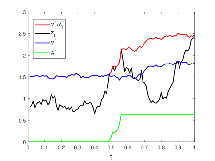
Figure 1: Sample paths of $t\to V_{t}^{*}$, $t\to Z_{t}$ and $t\to A_{t}^{*}$ via Monte Carlo simulation. The model parameters are set to be $\mathrm{v}=2,\leavevmode\nobreak\ z=0.8,\leavevmode\nobreak\ \rho=4,\leavevmode\nobreak\ \mu=1.5,\leavevmode\nobreak\ \sigma=2,\leavevmode\nobreak\ \mu_{Z}=1.7,\leavevmode\nobreak\ \sigma_{Z}=1,\leavevmode\nobreak\ \gamma=1,\leavevmode\nobreak\ \beta=2,\leavevmode\nobreak\ p=-\frac{\kappa}{1-\kappa}=-2.6357$.

We next present some structural properties satisfied by the optimal pair $(\theta^{*},c^{*})=(\theta^{*}_{t},c_{t}^{*})_{t\geq 0}$ of portfolio and consumption obtained in Theorem 4.1. To establish the structural properties of the optimal pair of investment and consumption, we focus on the case where the dimension of risky assets $d=1$ and the return rate $\mu>r=0$ as in Merton (1971).

The following lemma characterizes the asymptotic behavior of the optimal feedback control functions obtained in Theorem 4.1 when the initial wealth level tends to infinity.

Lemma 4.6.

Consider the optimal feedback control functions $\theta^{*}(x,z)$ and $c^{*}(x,z)$ for $(x,z)\in\mathds{R}_{+}\times(0,\infty)$ provided in Theorem 4.1. Then, for any $z>0$ fixed, and $\rho>\rho_{0}$ with $\rho_{0}>0$ given in (6.35), we have

$$\lim_{x\to+\infty}\frac{\theta^{*}(x,z)}{x} =\begin{cases}\displaystyle\frac{\mu}{\sigma^{2}(1-p)},&p>p_{1},\\[13.99995pt] \displaystyle\frac{1+C^{*}(1-\kappa)(1-p)\beta^{-(\kappa-1)}z}{1+C^{*}\beta^{-(\kappa-1)}z}\frac{\mu}{\sigma^{2}(1-p)}\\[10.00002pt] \displaystyle\qquad\quad+\frac{\sigma_{Z}}{\sigma}\frac{C^{*}\beta^{-(\kappa-1)}z}{1+C^{*}\beta^{-(\kappa-1)}z},&p=p_{1},\\[13.99995pt] \displaystyle(1-\kappa)\frac{\mu}{\sigma^{2}}+\frac{\sigma_{Z}}{\sigma},&p<p_{1},\end{cases}$$ (4.17)

and

$$\lim_{x\to+\infty}\frac{c^{*}(x,z)}{x} =\begin{cases}\displaystyle\leavevmode\nobreak\ \leavevmode\nobreak\ \leavevmode\nobreak\ \leavevmode\nobreak\ \leavevmode\nobreak\ \leavevmode\nobreak\ \leavevmode\nobreak\ C^{*},&p>p_{1},\\[10.00002pt] \displaystyle\frac{C^{*}}{1+C^{*}\beta^{-(1-\kappa)}z},&p=p_{1},\\[10.00002pt] \leavevmode\nobreak\ \leavevmode\nobreak\ \leavevmode\nobreak\ \leavevmode\nobreak\ \leavevmode\nobreak\ \leavevmode\nobreak\ \leavevmode\nobreak\ \leavevmode\nobreak\ 0,&p<p_{1}.\end{cases}$$ (4.18)

Here, the constant $C^{*}:=\frac{\rho(1-p)-\alpha p}{(1-p)^{2}}$ and $p_{1}\in(-\infty,0)$ is defined by

$$p_{1}:=-\frac{\kappa}{1-\kappa}.$$ (4.19)

Remark 4.7.

Based on Lemma 4.4 and Lemma 4.6, we have some further comparison discussions on our optimal tracking problem (2.4) and the classical Merton’s problem in Merton (1971):

• In the case $\mathrm{v}\geq z\geq 0,\leavevmode\nobreak\ \mu_{Z}=\sigma_{Z}=0$ and $\beta=+\infty$, (i.e., the benchmark process is always zero and the cost of capital injection is infinity), then the optimal tracking problem (2.4) degenerates into the Merton problem. Indeed, in this degenerate case, the equation $\alpha\kappa^{2}+(\rho-\eta-\alpha)\kappa+\mu_{Z}-\rho=0$ in Proposition 3.2 reduces to $\alpha\kappa^{2}+(\rho-\alpha)\kappa-\rho=0$, which yields that $\kappa=1$. As $\kappa=1$ and $\beta=+\infty$ in Eq. (4.6), we can see that, for all $x\geq 0$,

  $$x=\frac{(1-p)^{2}}{\rho(1-p)-\alpha p}f(x,z)^{-\frac{1}{1-p}}.$$ (4.20)

  Then, it follows from (4.20) and Corollary 4.2 that

  $$\theta^{*}(x,z)=\theta^{\rm{Mer}}(x):=\frac{\mu}{\sigma^{2}(1-p)}x,\quad c^{*}(x,z)=c^{\rm{Mer}}(x):=\frac{\rho(1-p)-\alpha p}{(1-p)^{2}}x,$$ (4.21)

  which is exactly the optimal solution of the classical Merton’s problem. Moreover, using (4.21), we can easily see that the local time $L_{t}=0$ for all $t\geq 0$, thus there is no capital injection in this case.

• In the case $\mathrm{v}\geq z\geq 0$, $\mu_{Z}=\sigma_{Z}=0$ and $\beta\in(0,+\infty)$, the benchmark is constant $z$, but the fund manager is still allowed to inject capital and the cost of capital injection is finite, we find that the optimal portfolio and consumption strategies differ from those in Merton’s problem. In fact, as in the above case (i), we still have $\kappa=1$ in Eq. (4.6). Hence, for all $x\geq 0$,

  $$x=\frac{(1-p)^{2}}{\rho(1-p)-\alpha p}\left(f(x,z)^{-\frac{1}{1-p}}-\beta^{-\frac{1}{1-p}}\right).$$ (4.22)

  Then, it follows from (4.20) and Corollary 4.2 that

  $$\begin{cases}\displaystyle\theta^{*}(x,z)=\theta^{\rm{Mer}}(x)+\underbrace{\frac{\mu}{\sigma^{2}}\frac{1-p}{\rho(1-p)-\alpha p}\beta^{-\frac{1}{1-p}}}_{\text{positive adjustment by capital injection}},\\[30.00005pt] \displaystyle c^{*}(x,z)=c^{\rm{Mer}}(x)+\underbrace{\qquad\beta^{-\frac{1}{1-p}}\qquad}_{\text{positive adjustment by capital injection}}.\end{cases}$$ (4.23)

  Although both the Merton problem without capital injection and our problem in (2.4) are solvable, due to the encouragement of risk-taking from the possible capital injection, the fund manager in our problem (2.4) adopts more aggressive optimal portfolio and consumption strategies with additional positive adjustment terms as shown in (4.21) and (4.23). It is also observed that these positive adjustments on the optimal portfolio and consumption strategies are independent of the wealth level. In particular, the adjustment term is decreasing w.r.t. the cost parameter $\beta$. When $\beta$ tends to infinity, it is clear that the impact of capital injection becomes vanishing and we therefore have $\lim_{\beta\to\infty}\theta^{*}(x,z)=\theta^{\rm{Mer}}(x)$ and $\lim_{\beta\to\infty}c^{*}(x,z)=c^{\rm{Mer}}(x)$ for all $x\geq 0$.

• In the case $\mathrm{v}\geq z>0$ and $\mu_{Z}>\eta$, the injection is indeed necessary for the agent in our optimal tracking problem (2.4). Lemma 4.4 shows this fact under the optimal strategy. For the general case, let us show it by contradiction. Assume that there exists a pair $(\theta^{M},c^{M})\in\mathbb{U}^{r}$ such that $V^{\theta^{M},c^{M}}_{t}\geq Z_{t}$, a.s., for all $t\in\mathds{R}_{+}$. Then we also have that $A^{\theta^{M},c^{M}}=0$ a.s., for all $t\in\mathds{R}_{+}$. Consider $(\tilde{V}^{\theta},\tilde{A}_{t}^{\theta})$ and $\tilde{\mathrm{w}}(\mathrm{v},z)$ defined in (6.39) and (6.40). Note that $c^{M}_{t}>0$ for all $t\in\mathds{R}_{+}$. Then, it follows from (2.2), (4.14) and (6.39) that $\tilde{V}_{t}^{\theta^{M}}\geq V^{\theta^{M},c^{M}}_{t}$ for all $t\in\mathds{R}_{+}$, and by (6.41), hence

  $$0<\tilde{\mathrm{w}}(\mathrm{v},z) =\inf_{\theta}\mathbb{E}\left[\int_{0}^{\infty}e^{-\rho t}d\tilde{A}_{t}^{\theta}\right]\leq\mathbb{E}\left[\int_{0}^{\infty}e^{-\rho t}d\tilde{A}_{t}^{\theta^{M}}\right]$$

  $$\leq\mathbb{E}\left[\int_{0}^{\infty}e^{-\rho t}dA^{\theta^{M},c^{M}}_{t}\right]=0,$$ (4.24)

  which yields the desired contradiction. That is, if we consider the classical Merton’s problem by requiring the strict benchmark outperforming constraint $V_{t}\geq Z_{t}$, a.s., for all $t\geq 0$, then the admissible set of Merton problem under the outperforming constraint is empty, i.e. there does not exist a pair $(\theta,c)\in\mathbb{U}^{r}$ such that $V^{\theta,c}_{t}\geq Z_{t}$, a.s., for all $t\geq 0$. Therefore, we have to consider the relaxed benchmark outperforming constraint using the strategic fictitious capital injection and allow the fund manager to be more risk-taking such that the wealth process is allowed to be negative from time to time.

In the next result, we examine the quantitative properties of $c^{*}(x,z)$ and $\theta^{*}(x,z)$ on the wealth variable $x\in\mathds{R}_{+}$.

Proposition 4.8.

Consider the optimal feedback control functions $\theta^{*}(x,z)$ and $c^{*}(x,z)$ for $(x,z)\in\mathds{R}_{+}\times(0,\infty)$ provided in Theorem 4.1. Then, for any $z>0$ fixed, and $\rho>\rho_{0}$ with $\rho_{0}>0$ given in (6.35), we have:

• $x\to c^{*}(x,z)$ is increasing;

• If $p\in(p_{1},1)$, $x\to c^{*}(x,z)$ is strictly convex; if $p\in(-\infty,p_{1})$, $x\to c^{*}(x,z)$ is strictly concave; and, if $p=p_{1}$, then $c^{*}(x,z)$ is linear in $x$;

• For the correlative coefficient $\gamma=1$, $x\to\theta^{*}(x,z)$ is increasing;

• For the correlative coefficient $\gamma=1$, if $p\in(-\infty,p_{1})\cup(p_{2},1)$, $x\to\theta^{*}(x,z)$ is strictly convex; if $p\in(p_{1},p_{2})$, $x\to\theta^{*}(x,z)$ is strictly concave; and, if $p=p_{1}$ or $p=p_{2}$, $\theta^{*}(x,z)$ is linear in $x$.

Here, $p_{1}$ is given in (4.19) and the critical point $p_{2}>p_{1}$ is given by

$$p_{2}:=\frac{\sigma\sigma_{Z}-\mu\kappa}{\mu(1-\kappa)+\sigma\sigma_{Z}}\in(-\infty,1).$$ (4.25)

We then have the following remarks on the results in Proposition 4.8.

Remark 4.9.

In the setting of utility maximization of consumption without benchmark tracking, Carroll and Kimball (1996) has discussed the concavity of the optimal feedback consumption function in terms of the wealth level induced by the income uncertainty. It was pointed out therein that the concavity of consumption can imply several interesting economic insights including the real-life observations that the financial risk-taking is often strongly related to wealth. However, it has also been shown in various extended models that the optimal consumption function may turn out to be convex within some wealth intervals when the consumption performance and risk-taking are affected by the past-average dependent habit formation (see Liu and Li (2023)), the consumption drawdown constraint (see Angoshtari et al. (2019) and Li et al. (2023)) or the possible negative terminal debt (see Chen and Vellekoop (2017)).

In our extended Merton problem, the risk aversion attitude from the utility function has been distorted by the relaxed benchmark tracking constraint. Indeed, the allowance of strategic capital injection not only enlarges the set of admissible controls, but also incentivizes the fund manager to be more risk-taking in choosing aggressive portfolio and consumption plans. From Proposition 4.8, one can observe that when the fund manager is very risk averse such that $p\leq p_{1}$, the risk aversion attitude from the utility function plays the dominant role and hence the optimal consumption functions exhibits concavity as observed in Carroll and Kimball (1996); when the fund manager is much less risk averse or close to risk neutral, i.e. $p>p_{1}$, the risk-taking component from the capital injection starts to distort the fund manager’s decision making, leading to convex optimal consumption function. In this case, when the wealth increases, the fund manager is willing to inject more capital to achieve the increasing marginal consumption.

5 Numerical Examples and Financial Implications

In addition to the quantitative properties with respect to wealth variable $x$ in Lemma 4.8, in this section, we will present some numerical examples to illustrate some other quantitative properties and financial implications of the optimal feedback control functions and the expectation of the discounted total capital injection. To ease the discussions, we only consider the case $d=1$ of the underlying stock in all examples.

First, to numerically illustrate the possible convexity and concavity of the optimal feedback portfolio and consumption functions resulting from different risk aversion parameter $p$ as stated in Proposition 4.8, we plot different cases in Figures 2 and 3 respectively. In particular, the increasing marginal portfolio (marginal consumption) shown in panel $(b)$ of Figure 2 (Figure 3) can be possibly explained by the increasing ratio between the marginal utility of portfolio (marginal utility of consumption) and the marginal capital injection.

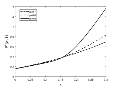
Figure 2: The optimal portfolio $x\to\theta^{*}(x,1)$. The model parameters are set to be $\rho=7,\leavevmode\nobreak\ \sigma=1,\leavevmode\nobreak\ \mu_{Z}=1,\leavevmode\nobreak\ \sigma_{Z}=1,\leavevmode\nobreak\ \gamma=1,\leavevmode\nobreak\ \beta=3$ and $\mu=0.1$ in Figure (a), $\mu=1$ in Figure (b).

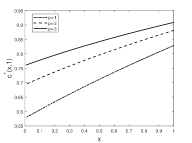
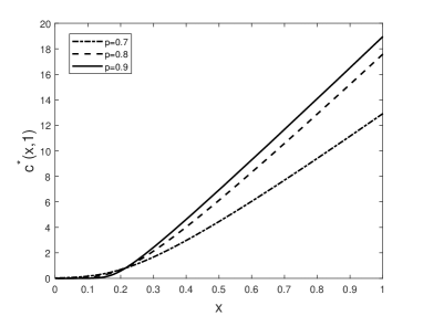
Figure 3: The optimal consumption $x\to c^{*}(x,1)$. The model parameters are set to be $\rho=7,\leavevmode\nobreak\ \mu=1,\leavevmode\nobreak\ \sigma=1,\leavevmode\nobreak\ \sigma_{Z}=1,\leavevmode\nobreak\ \gamma=1,\leavevmode\nobreak\ \beta=3$ and $\mu_{Z}=6.5$ in Figure (a), $\mu_{Z}=2$ in Figure (b)

We next illustrate in Figures 4 the sensitivity analysis of the optimal feedback portfolio and consumption as well as the expectation of the discounted capital injection with respect to the return parameter $\mu_{Z}$ in the benchmark dynamics. As expected, the expectation of the discounted capital injection is a decreasing function of the wealth variable $x$. More importantly, being consistent with the intuition, it is shown in Figure 4 that when the benchmark process has higher return, the fund manager will invest more in the risky asset and inject more capital to outperform the targeted benchmark, and meanwhile will strategically reduce the consumption amount due to the pressure of fulfilling the benchmark floor constraint.

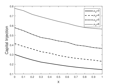
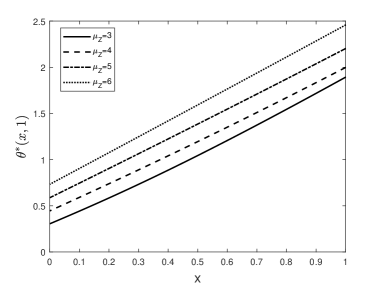
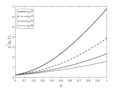
Figure 4: (a): The expectation of the total optimal discounted capital injection. (b): The optimal portfolio $x\to\theta^{*}(x,1)$. (c): The optimal consumption $x\to c^{*}(x,1)$. The model parameters are set to be $z=1,\leavevmode\nobreak\ \rho=8,\leavevmode\nobreak\ \mu=1,\leavevmode\nobreak\ \sigma=1,\leavevmode\nobreak\ \sigma_{Z}=1,\gamma=1,\leavevmode\nobreak\ p=0.5,\leavevmode\nobreak\ \beta=2$.

We then plot in Figure 5 the sensitivity results of the optimal feedback portfolio and consumption and the expectation of the discounted capital injection with respect to the cost parameter of capital injection. As $\beta$ increases, the fund manager is more hindered to inject capital and hence will strategically surpress the consumption plan to fulfil the benchmark constraint. Meanwhile, from panel $(b)$ of Figure 5, it is observed that the fund manager will also reduce the investment in the risky asset, which can be explained by the reduced volatility of the controlled wealth process that may help to avoid unnecessary capital injection in the tracking of the benchmark. More importantly, panel $(a)$ of Figure 5 shows that there is no monotonicity of the expected capital injection with respect to the cost parameter $\beta$ even when the wealth level is large. From a different perspective, it is possible to design the best choice of the cost parameter $\beta$ in our model such that the resulting expectation of discount capital injection can be minimized.

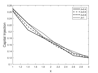
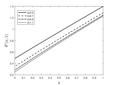
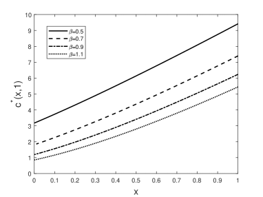
Figure 5: (a): The expectation of the total optimal discounted capital injection. (b): The optimal portfolio $x\to\theta^{*}(x,1)$. (c): The optimal consumption $x\to c^{*}(x,1)$. The model parameters are set to be $z=1,\leavevmode\nobreak\ \rho=5,\leavevmode\nobreak\ \mu=0.5,\leavevmode\nobreak\ \sigma=1,\leavevmode\nobreak\ \mu_{Z}=2,\leavevmode\nobreak\ \sigma_{Z}=1,\leavevmode\nobreak\ \gamma=1,\leavevmode\nobreak\ p=0.4$.

In Merton (1971), it has been shown that a more risk-averse agent would invest less wealth in the risky asset, see also further extensions to general utility functions in Borell (2007) and Xia (2011). As a sharp contrast, in Figure 6, we plot the optimal feedback portfolio and consumption functions with respect to the variable of risk aversion parameter $p$, illustrating that both $\theta^{*}$ and $c^{*}$ are not necessarily monotone in $p$ depending on different wealth regimes. These new and sophisticated phenomena are consequent on the fact that the risk aversion of the fund manager is distorted by the risk-taking from capital injection in our problem formulation to fulfil the benchmark constraint. When the wealth level is sufficiently large, the less risk averse (i.e. as $p$ tends to $1$) fund manager would invest and consume more aggressively; but when the wealth level is relatively low, the less risk averse fund manager has more concern on the cost of capital injection and will strategically reduce the portfolio and consumption plan.

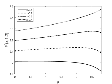
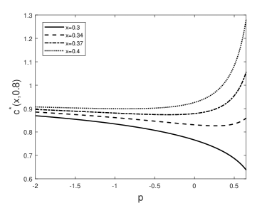
Figure 6: (a): The optimal portfolio $p\to\theta^{*}(x,1.2)$. The model parameters are set to be $\rho=5,\leavevmode\nobreak\ \mu=1,\leavevmode\nobreak\ \sigma=1,\leavevmode\nobreak\ \mu_{Z}=3,\leavevmode\nobreak\ \sigma_{Z}=1,\leavevmode\nobreak\ \gamma=1,\leavevmode\nobreak\ \beta=2$. (b): The optimal consumption $p\to c^{*}(x,0.8)$. The model parameters are set to be $\rho=5,\leavevmode\nobreak\ \mu=1,\leavevmode\nobreak\ \sigma=1,\leavevmode\nobreak\ \mu_{Z}=2,\leavevmode\nobreak\ \sigma_{Z}=1,\leavevmode\nobreak\ \gamma=1,\leavevmode\nobreak\ \beta=4$.

6 Proofs

This section collects all proofs of main results in previous sections.

Proof of Lemma 3.1.

Let $(x,z)\in\mathds{R}_{+}\times(0,\infty)$. For any $\epsilon>0$, denote by $(\theta^{\epsilon}(x,z),c^{\epsilon}(x,z)))\in\mathbb{U}^{\rm r}$ the $\epsilon$-optimal control strategy for (3.19) with the initial state $(x,z)$. In other words, it holds that

$$v(x,z)\leq J(x,z;\theta^{\epsilon}(x,z),c^{\epsilon}(x,z))+\epsilon.$$ (6.1)

Then, for any $x_{1}>x_{2}\geq 0$, we have from (6.1) that

$$v(x_{1},z)-v(x_{2},z) \geq J(x_{1},z;\theta^{\epsilon}(x_{2},z),c^{\epsilon}(x_{2},z))-J(x_{2},z;\theta^{\epsilon}(x_{2},z),c^{\epsilon}(x_{2},z))-\epsilon$$

$$=-\beta\mathbb{E}\left[\int_{0}^{\infty}e^{-\rho s}d(L_{s}^{x_{1}}-L_{s}^{x_{2}})\right]-\epsilon,$$ (6.2)

where $L_{s}^{x}$ for $s\in\mathds{R}_{+}$ is the local time process with $L_{0}^{x}=x$. Thus, integration by parts yields that, for all $T>0$,

$$\int_{0}^{T}e^{-\rho s}dL_{s}^{x}=e^{-\rho T}L_{T}^{x}-x+\rho\int_{0}^{T}L_{s}^{x}e^{-\rho s}ds.$$

Using the solution representation of “the Skorokhod problem”, it follows that, for all $s\geq 0$,

$$L_{s}^{x}=\sup_{\ell\in[0,s]}\left(x+\int_{0}^{\ell}\theta_{r}^{\top}\mu dr+\int_{0}^{\ell}\theta_{r}^{\top}\sigma dW_{r}-\int_{0}^{\ell}c_{r}dr-\int_{0}^{\ell}\mu_{Z}Z_{r}d{r}-\int_{0}^{\ell}\sigma_{Z}Z_{r}dW_{r}^{\gamma}\right)^{-}.$$

By this, we have $x\to L_{s}^{x}$ is non-increasing. Moreover, it holds that, $\mathbb{P}$-a.s.

$$\sup_{s\geq 0}\left|L_{s}^{x_{1}}-L_{s}^{x_{2}}\right|\leq|x_{1}-x_{2}|.$$ (6.3)

Using the fact $L_{s}^{x_{1}}-L_{s}^{x_{2}}\leq 0$ whenever $x_{1}>x_{2}\geq 0$, it follows from MCT that

$$\mathbb{E}\left[\int_{0}^{\infty}e^{-\rho s}d(L_{s}^{x_{1}}-L_{s}^{x_{2}})\right] =\lim_{T\to\infty}\mathbb{E}\left[\int_{0}^{T}e^{-\rho s}d(L_{s}^{x_{1}}-L_{s}^{x_{2}})\right]$$

$$=\lim_{T\to\infty}\left\{\mathbb{E}\left[e^{-\rho T}(L_{T}^{x_{1}}-L_{T}^{x_{2}})\right]+\rho\mathbb{E}\left[\int_{0}^{T}e^{-\rho s}(L_{s}^{x_{1}}-L_{s}^{x_{2}})ds\right]\right\}\leq 0.$$ (6.4)

Hence, we have from (6) that $v(x_{1},z)-v(x_{2},z)\geq-\epsilon$. Since $\epsilon>0$ is arbitrary, we get $v(x_{1},z)\geq v(x_{2},z)$. This conclude that $x\to v(x,z)$ is non-decreasing.

On the other hand, it follows from (6.3), (6) that

$$\left|v(x_{1},z)-v(x_{2},z)\right| \leq\beta\sup_{(\theta,c)\in\mathbb{U}^{\rm r}}\mathbb{E}\left[\int_{0}^{\infty}e^{-\rho s}d(L_{s}^{x_{2}}-L_{s}^{x_{1}})\right]$$

$$=\beta\sup_{(\theta,c)\in\mathbb{U}^{\rm r}}\lim_{T\to\infty}\mathbb{E}\left[e^{-\rho T}(L_{T}^{x_{2}}-L_{T}^{x_{1}})+\rho\int_{0}^{T}e^{-\rho s}(L_{s}^{x_{2}}-L_{s}^{x_{1}})ds\right]$$

$$\leq\beta\lim_{T\to\infty}\mathbb{E}\left[e^{-\rho T}|x_{1}-x_{2}|+\rho|x_{1}-x_{2}|\int_{0}^{T}e^{-\rho s}ds\right]$$

$$=\beta|x_{1}-x_{2}|.$$ (6.5)

Next, we fix $x\in\mathds{R}_{+}$. Let $L^{x,z}=(L_{t}^{x,z})_{t\geq 0}$ be the local time process of $X$ with $Z_{0}^{z}=z>0$ and $L_{0}^{x,z}=x$. Using the solution representation of “the Skorokhod problem” again, we can obtain that, for all $s\geq 0$,

$$\begin{cases}\displaystyle L_{s}^{x,z}=\sup_{\ell\in[0,s]}\left(x+\int_{0}^{\ell}\theta_{r}^{\top}\mu dr+\int_{0}^{\ell}\theta_{r}^{\top}\sigma dW_{r}-\int_{0}^{\ell}c_{r}dr-\int_{0}^{t}\mu_{Z}Z_{\ell}^{z}d{\ell}-\int_{0}^{t}\sigma_{Z}Z_{\ell}^{z}dW_{\ell}^{\gamma}\right)^{-},\\[11.99998pt] \displaystyle Z_{s}^{z}=z\exp\left[\left(\mu_{Z}-\frac{1}{2}\sigma_{Z}^{2}\right)s+\sigma_{Z}W^{\gamma}_{s}\right].\end{cases}$$

For any $z_{1},z_{2}>0$, by using BDG inequality and Jensen equality, it holds that

$$\mathbb{E}\left[\left|L_{s}^{x,z_{1}}-L_{s}^{x,z_{2}}\right|\right] \leq\mathbb{E}\left[\sup_{\ell\in[0,s]}\left|\int_{0}^{\ell}\mu_{Z}(Z_{r}^{1}-Z_{r}^{2})dr\right|\right]+\mathbb{E}\left[\sup_{\ell\in[0,s]}\left|\int_{0}^{\ell}\sigma_{Z}(Z_{r}^{1}-Z_{r}^{2})dW_{r}^{\gamma}\right|\right]$$

$$\leq|z_{1}-z_{2}||e^{\mu_{Z}s}-1|+3\sigma_{Z}\mathbb{E}\left[\left|\int_{0}^{s}(Z_{r}^{1}-Z_{r}^{2})^{2}dr\right|^{\frac{1}{2}}\right]$$

$$\leq|z_{1}-z_{2}||e^{\mu_{Z}s}-1|+3\sigma_{Z}\mathbb{E}\left[\int_{0}^{s}(Z_{r}^{1}-Z_{r}^{2})^{2}dr\right]^{\frac{1}{2}}$$

$$=\left[|e^{\mu_{Z}s}-1|+3\sigma_{Z}\left(\frac{e^{(2\mu_{Z}+\sigma_{Z}^{2})s}-1}{2\mu_{Z}+\sigma_{Z}^{2}}\right)^{\frac{1}{2}}\right]|z_{1}-z_{2}|.$$ (6.6)

Then, in a similar fashion, we can also show that, for all $(x,z_{1},z_{2})\in\mathds{R}_{+}^{3}$,

$$|v(x,z_{1})-v(x,z_{2})|\leq\beta\left(\sigma_{Z}^{2}+\frac{|\mu_{Z}|}{\rho-\mu_{Z}}+\frac{3}{\rho-2\mu_{Z}-\sigma_{Z}^{2}}\right)|z_{1}-z_{2}|.$$ (6.7)

Therefore, we deduce from (6.7) and (6.7) that

$$|v(x_{1},z_{1})-v(x_{2},z_{2})| \leq|v(x_{1},z_{1})-v(x_{2},z_{1})|+|v(x_{2},z_{1})-v(x_{2},z_{2})|$$

$$\leq\beta|x_{1}-x_{2}|+\beta\left(\sigma_{Z}^{2}+\frac{|\mu_{Z}|}{\rho-\mu_{Z}}+\frac{3}{\rho-2\mu_{Z}-\sigma_{Z}^{2}}\right)|z_{1}-z_{2}|.$$

Thus, we complete the proof of the lemma. ∎

Proof of Proposition 3.2.

It follows from the probabilistic representation (3.15) that we consider the candidate solution admitting the form $u(r,h)=l(r)+h\psi(r)$ for Eq. (3.14). In particular, the functions $r\to l(r)$ and $r\to\psi(r)$ satisfy the following equations, respectively:

$$-\rho l(r)+(\alpha-\rho)l_{r}(r)+\alpha l_{rr}(r)+\Phi(\beta e^{-r}) =0,$$ (6.8)

$$(\mu_{Z}-\rho)\psi(r)+(\alpha+\eta-\rho)\psi_{r}(r,h)+\alpha\psi_{rr}(r,h)-(\mu_{Z}-\eta)\beta e^{-r} =0.$$ (6.9)

By solving Eq.s (6.8) and (6.9), we obtain, for $p\in(-\infty,1)$,

$$l(r) =\begin{cases}\displaystyle\frac{(1-p)^{3}}{p(\rho(1-p)-\alpha p)}{\beta}^{-\frac{p}{1-p}}e^{\frac{p}{1-p}r}+C_{1}e^{-r}+C_{2}e^{\frac{\rho}{\alpha}r},&p\neq 0,\\[18.00005pt] \displaystyle\frac{1}{\rho}r-\frac{\ln\beta+2}{\rho}+\frac{\alpha}{\rho^{2}}+C_{1}e^{-r}+C_{2}e^{\frac{\rho}{\alpha}r},&p=0,\end{cases}$$

$$h(r) =\beta e^{-r}+C_{3}e^{-\kappa r}+C_{4}e^{-\hat{\kappa}r},$$

where $C_{i}$ with $i=1,\ldots,4$ are unknown real constants which will be determined later. Above, the constant $\kappa\in(0,1)$ is specified by (3.18), and the constant $\hat{\kappa}$ is given by

$$\hat{\kappa}:=\frac{-(\rho-\eta-\alpha)-\sqrt{(\rho-\eta-\alpha)^{2}+4\alpha(\rho-\mu_{Z})}}{2\alpha}<0.$$

Using the probability representation (3.15), we look for such functions $l(r)$ and $\psi(r)$ with $C_{2}=C_{4}=0$ and such that the Neumann boundary conditions $l^{\prime}(r)=0$ and $\psi^{\prime}(r)=0$ holds. This implies that

$$C_{1}=\frac{(1-p)^{2}}{\rho(1-p)-\alpha p}\beta^{-\frac{1}{1-p}},\quad C_{3}=-\frac{\beta}{\kappa}.$$

With the above specified constants $C_{i}$ with $i=1,\ldots,4$, we can easily verify that $u(r,h)=l(r)+h\psi(r)$ given by (3.19) satisfies Eq. (3.14). Thus, we complete the proof of the proposition. ∎

Proof of Theorem 4.1.

We first prove the item (i). For $(x,z)\in\mathds{R}_{+}\times(0,\infty)$, as (4.5), let $f(x,z)\in(0,\beta]$ satisfying $\hat{v}_{y}(f(x,z),z)=-x$. Then as (4.5), we have

$$v(x,z)=\inf_{y\in(0,\beta]}(\hat{v}(y,z)+yx)=\hat{v}(f(x,z),z)+xf(x,z).$$ (6.10)

Under the assumption that $\mu_{Z}\geq\eta$ and the quadratic equation (3.17) of $\kappa$, it is easy to see that $\mathcal{K}(1)=\mu_{Z}-\eta\geq 0$ and $\mathcal{K}(0)=\mu_{Z}-\rho<0$, where we define the mapping $\mathcal{K}(x)=\alpha x^{2}+(\rho-\eta-\alpha)x+\mu_{Z}-\rho$. Therefore, it follows that the root in (3.18) satisfies $\kappa\in(0,1]$. By applying the closed-form representation (4.1) of $\hat{v}$, it follows that, for the case $p\neq 0$,

$$\hat{v}_{y}(y,z) =\frac{(1-p)^{2}}{\rho(1-p)-\alpha p}\left(\beta^{-\frac{1}{1-p}}-y^{-\frac{1}{1-p}}\right)+z\left(1-\beta^{-(\kappa-1)}y^{\kappa-2}\right)\leq 0,\quad\forall y\in(0,\beta],$$

$$\hat{v}_{yy}(y,z) =\frac{1-p}{\rho(1-p)-\alpha p}y^{-\frac{1}{1-p}-1}+z(1-\kappa)\beta^{-(\kappa-1)}y^{\kappa-2}>0,\quad\forall y\in(0,\beta],$$

that is, the function $\hat{v}(y,z)$ is indeed convex in $y\in(0,\beta]$.

On the other hand, for the case $p=0$, it holds that

$$\hat{v}_{y}(y,z) =-\frac{1}{\rho y}+\frac{1}{\rho\beta}+z\left(1-\beta^{-(\kappa-1)}y^{\kappa-1}\right)\leq 0,\quad\forall y\in(0,\beta],$$

$$\hat{v}_{yy}(y,z) =\frac{1}{\rho y^{2}}+z(1-\kappa)\beta^{-(\kappa-1)}y^{\kappa-1}>0,\quad\forall y\in(0,\beta].$$

In summary, we have verified that $(0,\beta]\ni y\to\hat{v}(y,z)$ is indeed decreasing and strictly convex for any $z>0$ fixed. Moreover, since $\hat{v}_{y}(\beta,z)=0$, one has

$$\lim_{y\to 0}\hat{v}_{y}(y,z)=-\infty.$$

Thus, $f$ and $v$ defined by (4.2) is well-defined on $\mathds{R}_{+}\times(0,\infty)$. Therefore, using (6.10), a direct calculation yields that $v$ solves the primal HJB equation (3.8).

We next prove the item (ii). Note that the feedback control functions $(x,z)\to\theta^{*}(x,z)$ and $(x,z)\to c^{*}(x,z)$ given by (4.3) are continuous on $\mathds{R}_{+}\times(0,\infty)$. We then claim that, there exist a pair of positive constants $(M_{\theta},M_{c})$ such that, for all $(x,z)\in\mathds{R}_{+}\times(0,\infty)$,

$$|\theta^{*}(x,z)|\leq M_{\theta}(1+x+z),\quad|c^{*}(x,z)|\leq M_{c}(1+x+z).$$ (6.11)

In view of the duality transform, we arrive at $|c^{*}(x,z)|=f(x,z)^{\frac{1}{p-1}}$ and

$$|\theta^{*}(x,z)| \leq|(\sigma\sigma^{\top})^{-1}\mu|\left|\frac{v_{x}}{v_{xx}}(x,z)\right|+|\sigma_{Z}\gamma^{\top}\sigma^{-1}|\left|\frac{zv_{xz}}{v_{xx}}(x,z)\right|+|\sigma_{Z}\gamma^{\top}\sigma^{-1}|z$$ (6.12)

$$=|(\sigma\sigma^{\top})^{-1}\mu|f(x,z)\hat{v}_{yy}(f(x,z),z)+|\sigma_{Z}\gamma^{\top}\sigma^{-1}||z\hat{v}_{yz}(f(x,z),z)|+|\sigma_{Z}\gamma^{\top}\sigma^{-1}|z.$$

Moreover, it follows from the dual relationship (6.10) that $x=-v_{y}(f(x,z),z)$. For the case $p<1$ with $p\neq 0$, we have

$$y\hat{v}_{yy}(y,z) =\frac{1-p}{\rho(1-p)-\alpha p}y^{-\frac{1}{1-p}}+(1-\kappa)\beta^{-(\kappa-1)}zy^{\kappa-1},\quad z\hat{v}_{yz}(y,z)=z(1-\beta^{-(\kappa-1)}y^{\kappa-1}).$$

Thus, for all $y\in(\frac{\beta}{2},\beta]$ and $z>0$, it holds that $|f(x,z)^{\frac{1}{p-1}}|\leq(\frac{\beta}{2})^{\frac{1}{p-1}}$ and

$$y\hat{v}_{yy}(y,z) \leq\left(\frac{\beta}{2}\right)^{-\frac{1}{1-p}}+(1-\kappa)2^{1-\kappa}z,\quad|\hat{v}_{yz}(y,z)z|\leq(2^{1-\kappa}-1)z\leq z.$$ (6.13)

For the case $y\in(0,\frac{\beta}{2}]$ and $z>0$, we have

$$-\frac{y\hat{v}_{yy}(y,z)}{v_{y}(y,z)} =\frac{\frac{1-p}{\rho(1-p)-\alpha p}y^{-\frac{1}{1-p}}+(1-\kappa)\beta^{-(\kappa-1)}zy^{\kappa-1}}{\frac{(1-p)^{2}}{\rho(1-p)-\alpha p}(y^{-\frac{1}{1-p}}-\beta^{-\frac{1}{1-p}})+z\left(\beta^{-(\kappa-1)}y^{\kappa-1}-1\right)}$$

$$\leq\frac{\frac{1-p}{\rho(1-p)-\alpha p}y^{-\frac{1}{1-p}}}{\frac{(1-p)^{2}}{\rho(1-p)-\alpha p}(y^{-\frac{1}{1-p}}-\beta^{-\frac{1}{1-p}})}+\frac{(1-\kappa)\beta^{-(\kappa-1)}zy^{\kappa-1}}{z\left(\beta^{-(\kappa-1)}y^{\kappa-1}-1\right)}$$

$$\leq\frac{1}{(1-p)(1-2^{-\frac{1}{1-p}})}+\frac{1-\kappa}{1-2^{\kappa-1}},$$ (6.14)

$$-\frac{|z\hat{v}_{yz}(y,z)|}{v_{y}(y,z)} =\frac{(\beta^{-(\kappa-1)}y^{\kappa-1}-1)z}{\frac{(1-p)^{2}}{\rho(1-p)-\alpha p}(y^{-\frac{1}{1-p}}-\beta^{-\frac{1}{1-p}})+z\left(\beta^{-(\kappa-1)}y^{\kappa-1}-1\right)}\leq 1,$$ (6.15)

$$-\frac{y^{-\frac{1}{1-p}}}{v_{y}(y,z)} =\frac{y^{-\frac{1}{1-p}}}{\frac{(1-p)^{2}}{\rho(1-p)-\alpha p}(y^{-\frac{1}{1-p}}-\beta^{-\frac{1}{1-p}})+z\left(\beta^{-(\kappa-1)}y^{\kappa-1}-1\right)}$$

$$\leq\frac{1}{\frac{(1-p)^{2}}{\rho(1-p)-\alpha p}(1-\beta^{-\frac{1}{1-p}}y^{\frac{1}{1-p}})}\leq\frac{\rho(1-p)-\alpha p}{(1-p)^{2}}\frac{1}{1-2^{\frac{1}{1-p}}}.$$ (6.16)

For the case where $p=0$, we deduce that

$$y\hat{v}_{yy}(y,z) =\frac{1}{\rho y}+z(1-\kappa)\beta^{-(\kappa-1)}y^{\kappa-1},\quad\hat{v}_{yz}(y,z)=1-\beta^{-(\kappa-1)}y^{\kappa-1}.$$

Then, for all $y\in(\frac{\beta}{2},\beta]$ and $z>0$, it follows that $|f(x,z)^{-1}|\leq(\frac{\beta}{2})^{-1}$ and

$$y\hat{v}_{yy}(y,z) \leq\frac{2}{\rho\beta}+(1-\kappa)2^{1-\kappa}z,\quad|\hat{v}_{yz}(y,z)z|\leq(2^{1-\kappa}-1)z\leq z.$$ (6.17)

For $y\in(0,\frac{\beta}{2}]$ and $z>0$, we can obtain

$$-\frac{y\hat{v}_{yy}(y,z)}{v_{y}(y,z)} =\frac{\frac{1}{\rho y}+z(1-\kappa)\beta^{-(\kappa-1)}y^{\kappa-1}}{\frac{1}{\rho y}-\frac{1}{\rho\beta}+z\left(\beta^{-(\kappa-1)}y^{\kappa-1}-1\right)}=\frac{\beta}{\beta-y}+\frac{(1-\kappa)\beta^{-(\kappa-1)}}{\beta^{-(\kappa-1)}-y^{1-\kappa}}$$

$$\leq\frac{1}{2}+\frac{1-\kappa}{1-2^{\kappa-1}},$$ (6.18)

$$-\frac{|z\hat{v}_{yz}(y,z)|}{v_{y}(y,z)} =\frac{(\beta^{-(\kappa-1)}y^{\kappa-1}-1)z}{\frac{1}{\rho y}-\frac{1}{\rho\beta}+z\left(\beta^{-(\kappa-1)}y^{\kappa-1}-1\right)}\leq 1,$$ (6.19)

$$-\frac{|z\hat{v}_{yz}(y,z)|}{v_{y}(y,z)} =\frac{(\beta^{-(\kappa-1)}y^{\kappa-1}-1)z}{\frac{(1-p)^{2}}{\rho(1-p)-\alpha p}(y^{-\frac{1}{1-p}}-\beta^{-\frac{1}{1-p}})+z\left(\beta^{-(\kappa-1)}y^{\kappa-1}-1\right)}\leq 1,$$ (6.20)

$$-\frac{y^{-1}}{v_{y}(y,z)} =\frac{y^{-1}}{\frac{1}{\rho y}-\frac{1}{\rho\beta}+z(\beta^{-(\kappa-1)}y^{\kappa-1}-1)}\leq\frac{y^{-1}}{\frac{1}{\rho y}-\frac{1}{\rho\beta}}\leq 2\rho.$$ (6.21)

Therefore, by applying (6.12)-(6.21), we deduce that $|\theta^{*}(x,z)|\leq M_{\theta}(1+x+z)$ and $c^{*}(x,z)\leq M_{c}(1+x+z)$, where the positive constants $M_{\theta}$ and $M_{c}$ are defined respectively as

$$M_{\theta} :=|(\sigma\sigma^{\top})^{-1}\mu|\left[\left(\frac{\beta}{2}\right)^{-\frac{1}{1-p}}+(1-\kappa)2^{1-\kappa}+\frac{1}{(1-p)(1-2^{-\frac{1}{1-p}})}+\frac{1-\kappa}{1-2^{\kappa-1}}\right]+2|\sigma_{Z}\gamma^{\top}\sigma^{-1}|,$$ (6.22)

$$M_{c} :=\left(\frac{\beta}{2}\right)^{\frac{1}{p-1}}+\frac{\rho(1-p)-\alpha p}{(1-p)^{2}}\frac{1}{1-2^{\frac{1}{1-p}}}.$$ (6.23)

Hence, it follows from (6.11) that, for any $T>0$, SDE (4.4) satisfied by $X^{*}$ admits a weak solution on $[0,T]$ (c.f. Łaukajtys and Słomiński (2013)), which gives that $(\theta^{*},c^{*})\in\mathbb{U}^{\rm r}$.

On the other hand, fix $(T,x,z)\in(0,\infty)\times\mathds{R}_{+}\times(0,\infty)$ and $(\theta,c)\in\mathbb{U}^{\rm r}$. By applying Itô’s formula to $e^{-\rho T}v(X_{T},Z_{T})$, we arrive at

$$e^{-\rho T}v(X_{T},Z_{T})+\int_{0}^{T}e^{-\rho s}U(c_{s})ds$$

$$\quad=v(x,z)+\int_{0}^{T}e^{-\rho s}v_{x}(X_{s},Z_{s})\theta_{s}^{\top}\sigma dW_{s}+\int_{0}^{T}e^{-\rho s}\sigma_{Z}Z_{s}(v_{z}-v_{x})(X_{s},Z_{s})dW^{\gamma}_{s}$$

$$\qquad+\int_{0}^{T}e^{-\rho s}v_{x}(X_{s},Z_{s})dL_{s}^{X}+\int_{0}^{T}e^{-\rho s}({\cal L}^{\theta_{s},c_{s}}v-\rho v)(X_{s},Z_{s})ds,$$ (6.24)

where, for any $(\theta,c)\in\mathds{R}^{d}\times\mathds{R}_{+}$, the operator ${\cal L}^{\theta,c}$ acting on $C^{2}(\mathds{R}_{+}\times(0,\infty))$ is defined by

$${\cal L}^{\theta,c}g :=\theta^{\top}\mu g_{x}+\frac{1}{2}\theta^{\top}\sigma\sigma^{\top}\theta g_{xx}+\theta^{\top}\sigma\gamma\sigma_{Z}z(g_{xz}-g_{xx})+U(c)-cg_{x}$$

$$\quad-\sigma_{Z}^{2}z^{2}g_{xz}+\frac{1}{2}\sigma_{Z}^{2}z^{2}(g_{xx}+g_{zz})+\mu_{Z}z(g_{z}-g_{x}),\quad\forall g\in C^{2}(\mathds{R}_{+}\times(0,\infty)).$$

Taking the expectation on both sides of (6), we deduce from the Neumann boundary condition $v_{x}(0,z)=\beta$ that

$$\mathbb{E}\left[\int_{0}^{T}e^{-\rho s}U(c_{s})ds-\beta\int_{0}^{T}e^{-\rho s}dL_{s}\right]=v(x,z)-\mathbb{E}\left[e^{-\rho T}v(X_{T},Z_{T})\right]$$

$$\qquad\qquad+\mathbb{E}\left[\int_{0}^{T}e^{-\rho s}({\cal L}^{\theta_{s},c_{s}}v-\rho v)(X_{s},Z_{s})ds\right]\leq v(x,z)-\mathbb{E}\left[e^{-\rho T}v\left(X_{T},Z_{T}\right)\right].$$ (6.25)

Here, the last inequality in (6) holds true due to $({\cal L}^{\theta,c}v-\rho v)(x,z)\leq 0$ for all $(x,z)\in\mathds{R}_{+}\times(0,\infty)$ and $(\theta,c)\in\mathds{R}^{d}\times\mathds{R}_{+}$.

We next show the validity of the following transversality condition:

$$\limsup_{T\to\infty}\mathbb{E}\left[e^{-\rho T}v(X_{T},Z_{T})\right]\geq 0,$$ (6.26)

$$\lim_{T\to\infty}\mathbb{E}\left[e^{-\rho T}v(X_{T}^{*},Z_{T})\right]=0.$$ (6.27)

In view of (4.1), it follows that $x\to v(x,z)$ is non-decreasing. Thus, we get

$$\limsup_{T\to\infty}\mathbb{E}\left[e^{-\rho T}v(X_{T},Z_{T})\right]\geq\limsup_{T\to\infty}\mathbb{E}\left[e^{-\rho T}v(0,Z_{T})\right].$$ (6.28)

Using (4.1) again, it holds that $|v_{z}(x,z)|\leq(\frac{1}{\kappa}-1)\beta$ for all $(x,z)\in\mathds{R}_{+}\times(0,\infty)$. Therefore, for all $(x,z)\in\mathds{R}_{+}\times(0,\infty)$,

$$|v(0,z)| \leq|v(0,z)-v(0,0)|+|v(0,0)|\leq\left(\frac{1}{\kappa}-1\right)\beta z+|v(0,0)|.$$ (6.29)

Note that $\rho>\mu_{Z}$. Then, we can obtain

$$\lim_{T\to\infty}\mathbb{E}\left[e^{-\rho T}|v(0,Z_{T})|\right]\leq\left(\frac{1}{\kappa}-1\right)\beta\lim_{T\to\infty}e^{-\rho T}\mathbb{E}\left[Z_{T}\right]=\left(\frac{1}{\kappa}-1\right)\beta\lim_{T\to\infty}e^{-(\rho-\mu_{Z})T}=0.$$ (6.30)

So that, the desired result (6.26) follows from (6.28) and (6.30).

In terms of (4.1), one has $|v_{x}(x,z)|\leq\beta$ for all $(x,z)\in\mathds{R}_{+}\times(0,\infty)$. Hence, for all $(x,z)\in\mathds{R}_{+}\times(0,\infty)$,

$$|v(x,z)| \leq|v(x,z)-v(x,0)|+|v(x,0)-v(0,0)|+|v(0,0)|\leq\frac{\beta}{\kappa}\left(x+z\right)+|v(0,0)|.$$ (6.31)

For any $t\in\mathds{R}_{+}$, by applying Itô’s rule to $|X^{*}_{t}|^{2}$, we obtain

$$\mathbb{E}\left[|X_{t}^{*}|^{2}\right] =x^{2}+2\int_{0}^{t}\mathbb{E}\left[\theta^{*}(X_{s}^{*},Z_{s})^{\top}\mu X^{*}_{s}\right]ds+\int_{0}^{t}\mathbb{E}\left[\theta^{*}(X_{s}^{*},Z_{s})^{\top}\sigma\sigma^{\top}\theta^{*}(X_{s}^{*},Z_{s})\right]ds$$

$$\quad-2\int_{0}^{t}\mathbb{E}\left[c^{*}(X_{s}^{*},Z_{s})X_{s}^{*}\right]ds-\int_{0}^{t}\mathbb{E}\left[2\mu_{Z}Z_{s}X_{s}^{*}\right]ds+\sigma_{Z}^{2}\mathbb{E}\left[\int_{0}^{t}|Z_{s}|^{2}ds\right]$$

$$\quad-2\int_{0}^{t}\mathbb{E}\left[\theta^{*}(X_{s}^{*},Z_{s})^{\top}\sigma_{Z}\sigma\gamma Z_{s}\right]ds$$

$$\leq x^{2}+2\int_{0}^{t}\mathbb{E}\left[\theta^{*}(X_{s}^{*},Z_{s})^{\top}\mu X_{s}^{*}\right]ds+\int_{0}^{t}\mathbb{E}\left[\theta^{*}(X_{s}^{*},Z_{s})^{\top}\sigma\sigma^{\top}\theta^{*}(X_{s}^{*},Z_{s})\right]ds$$

$$\quad-\int_{0}^{t}\mathbb{E}\left[2\mu_{Z}Z_{s}X_{s}^{*}\right]ds+\sigma_{Z}^{2}\mathbb{E}\left[\int_{0}^{t}|Z_{s}|^{2}ds\right]-2\int_{0}^{t}\mathbb{E}\left[\theta^{*}(X_{s}^{*},Z_{s})^{\top}\sigma_{Z}\sigma\gamma Z_{s}\right]ds$$

$$\leq x^{2}+(4M_{\theta}|\mu|+2M_{\theta}^{2}|\sigma\sigma^{\top}|+|\mu_{Z}|+\sigma_{Z}^{2}+4M_{\theta}|\sigma_{Z}\sigma\gamma|)\int_{0}^{t}(1+\mathbb{E}[|X_{s}^{*}|^{2}]+\mathbb{E}[|Z_{s}|^{2}])ds$$

$$\leq x^{2}+2Kt(1+z^{2}e^{(2|\mu_{Z}|+3\sigma_{Z}^{2})t})+K\int_{0}^{t}\mathbb{E}[|X_{s}^{*}|^{2}]ds,$$ (6.32)

where the positive constant $K$ is specified as

$$K:=4M_{\theta}|\mu|+2M_{\theta}^{2}|\sigma\sigma^{\top}|+|\mu_{Z}|+\sigma_{Z}^{2}+4M_{\theta}|\sigma_{Z}\sigma\gamma|.$$ (6.33)

We then have from Gronwall’s inequality that, for all $t\in\mathds{R}_{+}$,

$$\mathbb{E}\left[|X_{t}^{*}|^{2}\right]\leq x^{2}+2Kt\left[1+Ke^{Kt}+z^{2}e^{(2|\mu_{Z}|+3\sigma_{Z}^{2})t}\left(1+\frac{Ke^{Kt}}{2|\mu_{Z}|+3\sigma_{Z}^{2}}\right)\right](1+x^{2}).$$ (6.34)

Let us define the following constant given by

$$\rho_{0}:=\frac{\alpha|p|+1}{1-p}+2|\mu_{Z}|+3\sigma_{Z}^{2}+K+1.$$ (6.35)

Then, using the estimates (6.31), (6) and (6.34), it follows that, for the discount rate $\rho>\rho_{0}$,

$$\lim_{T\to\infty}\mathbb{E}\left[e^{-\rho T}v(X_{T}^{*},Z_{T})\right]\leq\frac{\beta}{\kappa}\lim_{T\to\infty}\mathbb{E}\left[e^{-\rho T}(X_{T}^{*}+Z_{T})\right]=0.$$

Toward this end, letting $T\to\infty$ in (6), we obtain from (6.31) and DCT that, for all $(\theta,c)\in\mathbb{U}^{\rm r}$,

$$\mathbb{E}\left[\int_{0}^{\infty}e^{-\rho s}U(c_{s})ds-\beta\int_{0}^{\infty}e^{-\rho s}dL_{s}^{X}\right]\leq v(x,z),\quad\forall(x,z)\in\mathds{R}_{+}\times(0,\infty),$$

where the equality holds when $(\theta,c)=(\theta^{*},c^{*})$, and the proof of the theorem is completed. ∎

Proof of Lemma 4.4.

We first prove the item (i). For $(\mathrm{v},z)\in\mathds{R}_{+}\times(0,\infty)$, we have from (2.4) and Lemma 3.1 that

$$\beta\mathbb{E}\left[\int_{0}^{\infty}e^{-\rho t}dA^{*}_{t}\right] =\mathbb{E}\left[\int_{0}^{\infty}e^{-\rho t}U(c^{*}_{t})dt\right]-{\rm w}(\mathrm{v},z)-\beta(z-\mathrm{v})^{+}$$

$$=\mathbb{E}\left[\int_{0}^{\infty}e^{-\rho t}U(c^{*}_{t})dt\right]-v(x,z)$$

$$\leq\mathbb{E}\left[\int_{0}^{\infty}e^{-\rho t}U(c^{*}_{t})dt\right]+M(1+x+z),$$ (6.36)

where $M>0$ is a real constant depending on $(\mu,\sigma,\mu_{Z},\sigma_{Z},\gamma,p,\beta)$ and $x=(\mathrm{v}-z)^{+}$. In the sequel, we let $M>0$ be a generic positive constant dependent on $(\mu,\sigma,\mu_{Z},\sigma_{Z},\gamma,p,\beta)$, which may be different from line to line. Thus, in order to prove (4.13), it suffices to show that

$$\mathbb{E}\left[\int_{0}^{\infty}e^{-\rho t}U(c^{*}_{t})dt\right]<M(1+x+z).$$ (6.37)

In fact, by using (6), $\mathbb{E}[\int_{0}^{\infty}e^{-\rho t}U(c^{*}_{t})dt]$ can be not equal to $-\infty$ since ${\rm w}(\mathrm{v},z)$ is finite and $\beta\mathbb{E}[\int_{0}^{\infty}e^{-\rho t}dA^{*}_{t}]$ is nonnegative. The estimate (6.37) obviously holds for the case $p<0$ since $\mathbb{E}\left[\int_{0}^{\infty}e^{-\rho t}U(c^{*}_{t})dt\right]$ is negative in this case. Hence, we only focus on the case with $p\in[0,1)$. For $p\in(0,1)$, it follows from (6.11), (6.34) and the condition $\rho>\rho_{0}$ that

$$\mathbb{E}\left[\int_{0}^{\infty}e^{-\rho t}\frac{(c_{t}^{*})^{p}}{p}dt\right]\leq\frac{M_{c}^{p}}{p}\mathbb{E}\left[\int_{0}^{\infty}e^{-\rho t}(1+|X^{*}_{t}|+|Z_{t}|)^{p}dt\right]$$

$$\leq\frac{M_{c}^{p}}{p}\int_{0}^{\infty}e^{-\rho t}(1+\mathbb{E}[|X^{*}_{t}|]+\mathbb{E}[Z_{t}])dt\leq\frac{1}{p}(M_{c})^{p}\int_{0}^{\infty}e^{-\rho t}[1+\mu_{Z}tz+\mathbb{E}[|X^{*}_{t}|^{2}]^{\frac{1}{2}}]dt$$

$$\leq\frac{M_{c}^{p}}{p}\int_{0}^{\infty}e^{-\rho t}$$ (6.38)

$$\quad\times\left\{2+\mu_{Z}zt+\left(x^{2}+2Kt\left[1+Ke^{Kt}+z^{2}e^{(2|\mu_{Z}|+3\sigma_{Z}^{2})t}\left(1+\frac{Ke^{Kt}}{2|\mu_{Z}|+3\sigma_{Z}^{2}}\right)\right](1+x^{2})\right)^{\frac{1}{2}}\right\}dt$$

$$<M(1+x+z).$$

Here, $x=({\rm v}-z)^{+}$ via (3.19), and $M_{c}>0$ is the constant given by (6.23).

For the case with $p=0$, by using $\ln(x)<x$ for all $x>0$, and a similar discussion as (6), we can also get the estimate (6.37).

Next, we prove the item (ii). For any admissible portfolio $\theta=(\theta_{t})_{t\geq 0}$, let us introduce that, for all $t\in\mathds{R}_{+}$,

$$\tilde{V}_{t}^{\theta} =\textrm{v}+\int_{0}^{t}\theta_{s}^{\top}\mu ds+\int_{0}^{t}\theta_{s}^{\top}\sigma dW_{s},\quad\tilde{A}_{t}^{\theta}=0\vee\sup_{s\leq t}(Z_{s}-\tilde{V}^{\theta}_{s}).$$ (6.39)

Recall the optimal pair of investment and consumption $(\theta^{*},c^{*})=(\theta_{t}^{*},c_{t}^{*})_{t\geq 0}$ given by Theorem 4.1. Note that $c^{*}_{t}>0$ for all $t\in\mathds{R}_{+}$. Then, it follows from (2.2), (4.14) and (6.39) that $\tilde{V}_{t}^{\theta^{*}}\geq V^{\theta^{*},c^{*}}_{t}$ for all $t\in\mathds{R}_{+}$, and hence

$$\mathbb{E}\left[\int_{0}^{\infty}e^{-\rho t}dA^{*}_{t}\right]>\mathbb{E}\left[\int_{0}^{\infty}e^{-\rho t}d\tilde{A}_{t}^{\theta^{*}}\right]\geq\inf_{\theta}\mathbb{E}\left[\int_{0}^{\infty}e^{-\rho t}d\tilde{A}_{t}^{\theta}\right]=:\tilde{\mathrm{w}}(\mathrm{v},z).$$ (6.40)

It is not difficult to verify that, for all $(\mathrm{v},z)\in\mathds{R}_{+}\times(0,\infty)$,

$$\tilde{\mathrm{w}}(\mathrm{v},z)=z\frac{1-\kappa}{\kappa}\left(1+\frac{(\mathrm{v}-z)^{+}}{z}\right)^{\frac{\kappa}{\kappa-1}}>0,$$ (6.41)

where the constant $\kappa\in(0,1)$ is given by (3.18). Thus, we deduce from (6.40) and (6.41) that

$$\mathbb{E}\left[\int_{0}^{\infty}e^{-\rho t}dA^{*}_{t}\right]\geq z\frac{1-\kappa}{\kappa}\left(1+\frac{(\mathrm{v}-z)^{+}}{z}\right)^{\frac{\kappa}{\kappa-1}}>0,$$ (6.42)

which completes the proof. ∎

Proof of Lemma 4.6.

It follows from the duality relationship that $x=-\hat{v}_{y}(y,z)$ and

$$\theta^{*}(x,z) =-\frac{\mu}{\sigma^{2}}\frac{v_{x}}{v_{xx}}(x,z)-\frac{\sigma_{Z}}{\sigma}\left(\frac{zv_{xz}}{v_{xx}}(x,z)-z\right)$$

$$=\frac{\mu}{\sigma^{2}}f(x,z)\hat{v}_{yy}(f(x,z),z)-\frac{\sigma_{Z}}{\sigma}(z\hat{v}_{yz}(f(x,z),z)-z).$$ (6.43)

Hence, we have from (6) that

$$\lim_{x\to+\infty}\frac{\theta^{*}(x,z)}{x} =\lim_{x\to+\infty}\frac{\mu f(x,z)\hat{v}_{yy}(f(x,z),z)-\sigma_{Z}\sigma(z\hat{v}_{yz}(f(x,z),z)-z)}{-\sigma^{2}\hat{v}_{y}(f(x,z),z)}$$

$$=\lim_{y\to 0}\frac{\mu y\hat{v}_{yy}(y,z)-\sigma_{Z}\sigma z\hat{v}_{yz}(y,z)}{-\sigma^{2}\hat{v}_{y}(y,z)}.$$ (6.44)

By using (4.1), for $p<1$ with $p\neq 0$, it holds that

$$\lim_{y\to 0}\frac{y\hat{v}_{yy}(y,z)}{-v_{y}(y,z)} =\lim_{x\to+\infty}\frac{\frac{1-p}{\rho(1-p)-\alpha p}y^{-\frac{1}{1-p}}+(1-\kappa)\beta^{-(\kappa-1)}zy^{\kappa-1}}{\frac{(1-p)^{2}}{\rho(1-p)-\alpha p}(y^{-\frac{1}{1-p}}-\beta^{-\frac{1}{1-p}})+z\left(\beta^{-(\kappa-1)}y^{\kappa-1}-1\right)}$$

$$=\lim_{y\to 0}\frac{\frac{1-p}{\rho(1-p)-\alpha p}+(1-\kappa)\beta^{-(\kappa-1)}zy^{\kappa-1+\frac{1}{1-p}}}{\frac{(1-p)^{2}}{\rho(1-p)-\alpha p}(1-\beta^{-\frac{1}{1-p}}y^{\frac{1}{1-p}})+z\left(\beta^{-(\kappa-1)}y^{\kappa-1+\frac{1}{1-p}}-y^{\frac{1}{1-p}}\right)}$$

$$=\frac{1}{1-p}\lim_{y\to 0}\frac{1+C^{*}(1-\kappa)(1-p)\beta^{-(\kappa-1)}zy^{\kappa+\frac{p}{1-p}}}{1+zC^{*}\beta^{-(\kappa-1)}y^{\kappa+\frac{p}{1-p}}},$$ (6.45)

$$\lim_{y\to 0}\frac{z\hat{v}_{yz}(y,z)}{-v_{y}(y,z)} =\lim_{y\to 0}\frac{(\beta^{-(\kappa-1)}y^{\kappa-1}-1)z}{\frac{(1-p)^{2}}{\rho(1-p)-\alpha p}(y^{-\frac{1}{1-p}}-\beta^{-\frac{1}{1-p}})+z\left(\beta^{-(\kappa-1)}y^{\kappa-1}-1\right)}$$

$$=\lim_{y\to 0}\frac{(\beta^{-(\kappa-1)}y^{\kappa+\frac{p}{1-p}}-y^{\frac{1}{1-p}})z}{\frac{(1-p)^{2}}{\rho(1-p)-\alpha p}(1-\beta^{-\frac{1}{1-p}}y^{\frac{1}{1-p}})+z\left(\beta^{-(\kappa-1)}y^{\kappa+\frac{p}{1-p}}-y^{\frac{1}{1-p}}\right)}$$

$$=\lim_{y\to 0}\frac{C^{*}\beta^{-(\kappa-1)}y^{\kappa+\frac{p}{1-p}}z}{1+C^{*}\beta^{-(\kappa-1)}y^{\kappa+\frac{p}{1-p}}z}.$$ (6.46)

By discussing the three cases of $p>p_{1}$, $p=p_{1}$ and $p<p_{1}$, respectively, we can deduce the desired result (4.17) following from (6.45) and (6.46). Furthermore, we can easily verify that the limit (4.17) also holds true for the case with $p=0$.

Next, it follows from the relationship $x=-\hat{u}_{y}(y,z)$ and (4.1) that, for $p<1$ with $p\neq 0$,

$$\lim_{x\to+\infty}\frac{c^{*}(x,z)}{x} =\lim_{x\to+\infty}\frac{f(x,z)^{\frac{1}{1-p}}}{-\hat{v}_{y}(f(x,z),z)}=\lim_{y\to 0}\frac{y^{\frac{1}{1-p}}}{-\hat{v}_{y}(y,z)}$$

$$=\lim_{y\to 0}\frac{y^{-\frac{1}{1-p}}}{\frac{(1-p)^{2}}{\rho(1-p)-\alpha p}(y^{-\frac{1}{1-p}}-\beta^{-\frac{1}{1-p}})+z\left(\beta^{-(\kappa-1)}y^{\kappa-1}-1\right)}$$

$$=\lim_{y\to 0}\frac{C^{*}}{(1-\beta^{-\frac{1}{1-p}}y^{\frac{1}{1-p}})+zC^{*}\left(\beta^{-(\kappa-1)}y^{\kappa+\frac{p}{1-p}}-y^{\frac{1}{1-p}}\right)}$$

$$=\lim_{y\to 0}\frac{C^{*}}{1+C^{*}\beta^{-(\kappa-1)}y^{\kappa+\frac{p}{1-p}}z}.$$ (6.47)

Thanks to (6), we can obtain the desired result (4.18) via a direct calculation, which also holds for the case $p=0$. ∎

Proof of Lemma 4.8.

We first prove the item (i). For $(x,z)\in\mathds{R}_{+}\times(0,\infty)$, recall that $f(x,z)\in(0,\beta]$ satisfying the following equation:

$$\hat{v}_{y}(f(x,z),z)=-x.$$ (6.48)

Taking the derivative with respect to $x$ on the both sides of (6.48), we deduce that

$$f_{x}(x,z)=-\frac{1}{\hat{v}_{yy}(f(x,z),z)}.$$ (6.49)

Then, it follows from (3.15) and (6.49) that

$$\frac{\partial c^{*}(x,z)}{\partial x}=\frac{\partial f(x,z)^{\frac{1}{p-1}}}{\partial x}=\frac{1}{p-1}f(x,z)^{\frac{1}{p-1}-1}f_{x}(x,z)=\frac{f(x,z)^{\frac{1}{p-1}-1}}{(1-p)\hat{v}_{yy}(f(x,z),z)}>0.$$ (6.50)

This implies that $x\to c^{*}(x,z)$ is increasing.

Next, we deal with the item (ii). Taking the derivative with respect to $x$ on the both sides of (6.49) again, we obtain

$$f_{xx}(x,z)=\frac{1}{\hat{v}^{2}_{yy}(f(x,z),z)}\hat{v}_{yyy}(f(x,z),z)f_{x}(x,z)=-\frac{\hat{v}_{yyy}(f(x,z),z)}{\hat{v}^{3}_{yy}(f(x,z),z)}.$$ (6.51)

Hence, it follows from (3.15), (6.50) and (6.51) that

$$\frac{\partial^{2}c^{*}(x,z)}{\partial x^{2}} =\frac{1}{p-1}f(x,z)^{\frac{2-p}{p-1}}f_{xx}(x,z)+\frac{2-p}{(p-1)^{2}}f(x,z)^{\frac{3-2p}{p-1}}f_{x}(x,z)^{2}$$

$$=-\frac{1}{p-1}f(x,z)^{\frac{2-p}{p-1}}\frac{\hat{v}_{yyy}(f(x,z),z)}{\hat{v}^{3}_{yy}(f(x,z),z)}+\frac{2-p}{(p-1)^{2}}f(x,z)^{\frac{3-2p}{p-1}}\frac{1}{\hat{v}^{2}_{yy}(f(x,z),z)}$$

$$=\frac{1}{1-p}\frac{f(x,z)^{\frac{3-2p}{p-1}}}{\hat{v}^{3}_{yy}(f(x,z),z)}\left[f(x,z)\hat{v}_{yyy}(f(x,z),z)+\frac{2-p}{1-p}\hat{v}_{yy}(f(x,z),z)\right].$$ (6.52)

We then obtain from (4.1) and (6) that

$$\frac{\partial^{2}c^{*}(x,z)}{\partial x^{2}} =\frac{1-\kappa}{1-p}\frac{f(x,z)^{\frac{3-2p}{p-1}+\kappa-1}}{\hat{v}^{3}_{yy}(f(x,z),z)}\beta^{-(\kappa-1)}z\left(\kappa+\frac{p}{1-p}\right),$$ (6.53)

which implies the desired item (ii).

Toward this end, we move to the proof of the item (iii). By applying Theorem 4.1, it holds that

$$\theta^{*}(x,z) =-\frac{\mu}{\sigma^{2}}\frac{v_{x}}{v_{xx}}(x,z)-\frac{\sigma_{Z}}{\sigma}\left(\frac{zv_{xz}}{v_{xx}}(x,z)-z\right)$$

$$=\frac{\mu}{\sigma^{2}}f(x,z)\hat{v}_{yy}(f(x,z),z)-\frac{\sigma_{Z}}{\sigma}(z\hat{v}_{yz}(f(x,z),z)-z).$$

This yields that

$$\frac{\partial\theta^{*}(x,z)}{\partial x}$$

$$\quad=f_{x}(x,z)\left(\frac{\mu}{\sigma^{2}}\left(\hat{v}_{yy}(f(x,z),z)+f(x,z)\hat{v}_{yyy}(f(x,z),z)\right)-\frac{\sigma_{Z}}{\sigma}z\hat{v}_{yyz}(f(x,z),z)\right).$$ (6.54)

In lieu of (4.1), we can see that

$$(\hat{v}_{yy}+y\hat{v}_{yyy})(y,z) =-\frac{1}{\rho(1-p)-\alpha p}y^{\frac{2-p}{p-1}}-z(1-\kappa)^{2}\beta^{-\kappa-1)}y^{\kappa-2},$$ (6.55)

$$\hat{v}_{yyz}(y,z) =(1-\kappa)\beta^{-\kappa-1)}y^{\kappa-2}.$$ (6.56)

Then, from (6), (6.55) and (6.56), we deduce that

$$\frac{\partial\theta^{*}(x,z)}{\partial x} =\frac{\mu}{\sigma^{2}}\frac{f(x,z)^{\kappa-2}}{\hat{v}_{yy}(f(x,z),z)}$$

$$\quad\times\left[\frac{1}{\rho(1-p)-\alpha p}f(x,z)^{-(\frac{p}{1-p}+\kappa)}+(1-\kappa)\beta^{-(\kappa-1)}z\left(1-\kappa+\frac{\sigma_{Z}\sigma}{\mu}\right)\right].$$ (6.57)

Note that $\frac{\partial\theta^{*}(x,z)}{\partial x}>0$ for all $x\in\mathds{R}_{+}$. Then, we obtain that $x\to\theta^{*}(x,z)$ is increasing.

Finally, it remains to prove the item (iv). In fact, it follows from (6) that

$$\frac{\partial^{2}\theta^{*}(x,z)}{\partial x^{2}}=-\frac{\mu}{\sigma^{2}}\frac{1}{\hat{v}^{2}_{yy}(f(x,z),z)}$$

$$\leavevmode\nobreak\ \times\left[\frac{1}{\rho(1-p)-\alpha p}\frac{2-p}{p-1}f(x,z)^{\frac{3-2p}{p-1}}+f(x,z)^{\kappa-3}(1-\kappa)(\kappa-2)\beta^{-(\kappa-1)}z\left(1-\kappa+\frac{\sigma_{Z}\sigma}{\mu}\right)\right]$$

$$\leavevmode\nobreak\ +\frac{\mu}{\sigma^{2}}\frac{\hat{v}_{yyy}(f(x,z),z)}{\hat{v}^{3}_{yy}(f(x,z),z)}\left[\frac{1}{\rho(1-p)-\alpha p}f(x,z)^{\frac{2-p}{p-1}}+f(x,z)^{\kappa-2}(1-\kappa)\beta^{-(\kappa-1)}z\left(1-\kappa+\frac{\sigma_{Z}\sigma}{\mu}\right)\right]$$

$$\leavevmode\nobreak\ =\frac{\mu}{\sigma^{2}}\frac{1}{\hat{v}^{3}_{yy}(f(x,z),z)}\left[\frac{1}{\rho(1-p)-\alpha p}f(x,z)^{\frac{3-2p}{p-1}}\left(\frac{2-p}{1-p}\hat{v}_{yy}(f(x,z),z)+f(x,z)\hat{v}_{yyy}(f(x,z),z)\right)\right.$$

$$\leavevmode\nobreak\ +\left.f(x,z)^{\kappa-3}(1-\kappa)\beta^{-(\kappa-1)}z\left(1-\kappa+\frac{\sigma_{Z}\sigma}{\mu}\right)\left((2-\kappa)\hat{v}_{yy}(f(x,z),z)+f(x,z)\hat{v}_{yyy}(f(x,z),z)\right)\right]$$

$$\leavevmode\nobreak\ =\frac{\mu}{\sigma^{2}}\frac{\beta^{-(\kappa-1)}(1-\kappa)z}{\hat{v}_{yy}^{3}(f(x,z),z)}\frac{1-p}{\rho(1-p)-\alpha p}f(x,z)^{-\frac{5-4p}{p-1}+\kappa}\left(\frac{p}{1-p}+\kappa\right)\left(\frac{p}{1-p}+\kappa-\frac{\sigma\sigma_{Z}}{\mu}\right).$$ (6.58)

Note that, it holds that

$$\left(\frac{p}{1-p}+\kappa\right)\left(\frac{p}{1-p}+\kappa-\frac{\sigma\sigma_{Z}}{\mu}\right)\begin{cases}\displaystyle>0,&\text{if}\leavevmode\nobreak\ p\in(\infty,p_{1})\cup(p_{2},1);\\[8.00003pt] \displaystyle=0,&\text{if}\leavevmode\nobreak\ p=p_{1}\leavevmode\nobreak\ \text{or}\leavevmode\nobreak\ p=p_{2};\\[8.00003pt] \displaystyle<0,&\text{if}\leavevmode\nobreak\ p\in(p_{1},p_{2}).\end{cases}$$ (6.59)

The desired result (iv) follows from (6) and (6.59). ∎

Acknowledgements The authors would like to thank Martin Larsson and Johannes Ruf for proposing the relaxed benchmarking tracking using the capital injection during their visit to the Hong Kong Polytechnic University in 2018. L. Bo and Y. Huang are supported by National Key R&D Program of China under grant no. 2022YFA1000033 and National Natural Science Foundation of China under grant no. 11971368. X. Yu is supported by the Hong Kong RGC General Research Fund (GRF) under grant no. 15304122 and the Hong Kong Polytechnic University research grant under no. P0039251.

References

- Angoshtari et al. (2019) B. Angoshtari, E. Bayraktar and V. R. Young (2019): Optimal dividend distribution under drawdown and ratcheting constraints on dividend rates. SIAM J. Financial Math. 10(2), 547-577.
- Barles et al. (1994) G. Barles, C. Daher and M. Romano (1994): Optimal control on the norm of a diffusion process. SIAM J. Contr. Optim. 32(3), 612-634.
- Barron and Ishii (1989) E. N. Barron and H. Ishii (1989): The Bellman equation for minimizing the maximum cost. Nonlinear Anal.: TMA 13(9), 1067-1090.
- Bo et al. (2021) L. Bo, H. Liao and X. Yu (2021): Optimal tracking portfolio with a ratcheting capital benchmark. SIAM J. Control. Optim. 59(3), 2346-2380.
- Bo et al. (2023) L. Bo, Y. Huang and X. Yu (2023): A stochastic control problem arising from relaxed wealth tracking with a monotone benchmark process. Preprint, arXiv:2302.08302.
- Bokanowski et al. (2015) O. Bokanowski, A. Picarelli and H. Zidani (2015): Dynamic programming and error estimates for stochastic control problems with maximum cost. Appl. Math. Optim. 71, 125-163.
- Borell (2007) C. Borell (2007): Monotonicity properties of optimal investment strategies for log-Brownian asset prices. Math. Finan. 17(1), 143-153.
- Boyle and Tian (2007) P. Boyle and W. Tian (2007): Portfolio management with constraints. Math. Finan. 17(3), 319-343.
- Browne (1999a) S. Browne (1999a): Reaching goals by a deadline: Digital options and continuous-time active portfolio management. Adv. Appl. Prob. 31, 551-577.
- Browne (1999b) S. Browne (1999b): Beating a moving target: Optimal portfolio strategies for outperforming a stochastic benchmark. Finan. Stoch. 3, 275-294.
- Browne (2000) S. Browne (2000): Risk-constrained dynamic active portfolio management Manag. Sci. 46(9), 1188-1199.
- Carroll and Kimball (1996) C. D. Carroll and M. S. Kimball (1996): On the concavity of the consumption function. Econometrica. 64(4), 981-992.
- Chen and Vellekoop (2017) A. Chen and M. Vellekoop (2017): Optimal investment and consumption when allowing terminal debt. Euro. J. Oper. Res. 258, 385-397.
- Chow et al. (2020) Y. Chow, X. Yu and C. Zhou (2020): On dynamic programming principle for stochastic control under expectation constraints. J. Optim. Theor. Appl. 185(3), 803-818.
- Deng et al. (2022) S. Deng, X. Li, H. Pham and X. Yu (2022): Optimal consumption with reference to past spending maximum. Finan. Stoch. 26, 217-266.
- Gaivoronski et al. (2005) A. Gaivoronski, S. Krylov and N. Wijst (2005): Optimal portfolio selection and dynamic benchmark tracking. Euro. J. Oper. Res. 163, 115-131.
- Di Giacinto et al. (2011) M. Di Giacinto, S. Federico and F. Gozzi (2011): Pension funds with a minimum guarantee: a stochastic control approach. Finan. Stoch. 15, 297-342.
- Guasoni et al. (2011) P. Guasoni, G. Huberman and Z. Y. Wang (2011): Performance maximization of actively managed funds. J. Financial Econom. 101, 574-595.
- El Karoui et al. (2005) N. El Karoui, M. Jeanblanc and V. Lacoste (2005): Optimal portfolio management with American capital guarantee. J. Econ. Dyn. Contr. 29, 449-468.
- El Karoui and Meziou (2006) N. El Karoui and A. Meziou (2006): Constrained optimization with respect to stochastic dominance: application to portfolio insurance. Math. Finan. 16(1), 103-117.
- Li et al. (2023) X. Li, X. Yu and Q. Zhang (2023): Optimal consumption and life insurance under shortfall aversion and a drawdown constraint. Insur.: Math. Econ. 108, 25-45.
- Liu and Li (2023) H. Liu and L. Li (2023): On the concavity of consumption function under habit formation. J. Math. Econ. 106, 102829.
- Ni et al. (2022) C. Ni, Y. Li, P. Forsyth and R. Carroll (2022): Optimal asset allocation for outperforming a stochastic benchmark target. Quant. Finance 22(9), 1595-1626.
- Kröner et al. (2018) A. Kröner, A. Picarelli and H. Zidani (2018): Infinite horizon stochastic optimal control problems with running maximum cost. SIAM J. Contr. Optim. 56(5), 3296-3319.
- Łaukajtys and Słomiński (2013) W. Łaukajtys and L. Słomiński (2013): Penalization methods for the Skorokhod problem and reflecting SDEs with jumps. Bernoulli. 19(5A), 1750-1775.
- Merton (1969) R. C. Merton (1969): Lifetime portfolio selection under uncertainty: the continuous time case. Rev. Econ. Stat. 51(3), 247-257.
- Merton (1971) R. C. Merton (1971): Optimum consumption and portfolio rules in a continuous-time model. J. Econ. Theor. 3(4), 373-413.
- Pham (2002) H. Pham (2002): Minimizing shortfall risk and applications to finance and insurance problems. Ann. Appl. Probab. 12(1), 143-172.
- Sekine (2012) J. Sekine (2012): Long-term optimal portfolios with floor. Finan. Stoch. 16, 369-401.
- Strub and Baumann (2018) O. Strub and P. Baumann (2018): Optimal construction and rebalancing of index-tracking portfolios. Euro. J. Oper. Res. 264, 370-387.
- Weerasinghe and Zhu (2016) A. Weerasinghe and C. Zhu (2016): Optimal inventory control with path-dependent cost criteria. Stoch. Process. Appl. 126, 1585-1621.
- Xia (2011) J. Xia (2011): Risk aversion and portfolio selection in a continuous-time model. SIAM J. Contr. Optim. 49(5), 1916-1937.
- Yao et al. (2006) D. Yao, S. Zhang and X. Zhou (2006): Tracking a financial benchmark using a few assets. Oper. Res. 54(2), 232-246.