Protection Against Graph-Based False Data Injection Attacks on Power Systems

Abstract

Graph signal processing (GSP) has emerged as a powerful tool for practical network applications, including power system monitoring. Recent research has focused on developing GSP-based methods for state estimation, attack detection, and topology identification using the representation of the power system voltages as smooth graph signals. Within this framework, efficient methods have been developed for detecting false data injection (FDI) attacks, which until now were perceived as non-smooth with respect to the graph Laplacian matrix. Consequently, these methods may not be effective against smooth FDI attacks. In this paper, we propose a graph FDI (GFDI) attack that minimizes the Laplacian-based graph total variation (TV) under practical constraints. We present the GFDI attack as the solution for a non-convex constrained optimization problem. The solution to the GFDI attack problem is obtained through approximating it using $\ell_{1}$ relaxation. A series of quadratic programming problems that are classified as convex optimization problems are solved to obtain the final solution. We then propose a protection scheme that identifies the minimal set of measurements necessary to constrain the GFDI output to a high graph TV, thereby enabling its detection by existing GSP-based detectors. Our numerical simulations on the IEEE-$57$ and IEEE-$118$ bus test cases reveal the potential threat posed by well-designed GSP-based FDI attacks. Moreover, we demonstrate that integrating the proposed protection design with GSP-based detection can lead to significant hardware cost savings compared to previous designs of protection methods against FDI attacks.

I Introduction

Power system state estimation (PSSE) is a crucial component of modern energy management systems (EMSs) that fulfills various purposes, including monitoring, analysis, security, control, and management of power delivery [1]. PSSE is conducted using power measurements to estimate the voltages (states) at the system buses. To ensure the reliability of the measurements, residual-based bad data detection (BDD) methods are integrated into the EMS [1]. However, BDD methods are not able to detect well-designed attacks, known as unobservable false data injection (FDI) attacks [2, 3], which can cause significant damage by misleading the PSSE system[4, 5, 6]. These attacks are achieved by manipulating measurements based on the power network topology [2], where the topology matrix is either known or can be estimated from historical data [7, 8, 9, 10].

Defending power systems against unobservable FDI attacks involves two primary approaches. The first approach is to prevent attacks by protecting a subset of measurements using techniques such as encryption, continuous monitoring, and separation from the Internet [11]. This often involves identifying a minimal set of measurements required to prevent an adversary from constructing a feasible sparse FDI attack [12, 13, 11, 14, 15]. These works aim to ensure network observability and maintain the grid’s immunity to well-coordinated attacks. Synchronized phasor measurement unit (PMU) placement has also been suggested for the optimal deployment of protective measurements [11, 16, 17, 18]. However, current methodologies do not consider recent developments of graph signal processing (GSP)-based detectors against FDI. The second main approach to protect power systems is to develop detection methods against unobservable FDI attacks that rely on system characteristics. These methods include compressive sensing algorithms [19, 20, 21, 22] that require certain structural properties for the system powers and a differential model with multi-time measurements. Another detection technique is the moving target defense [23], where the system configuration is actively changed. Detection and identification methods based on machine learning, Kalman filters, and data mining have also been suggested [24, 25, 26, 27, 28, 29, 30, 31]. However, these data-driven methods require a large set of historical and real-time power system data, which is usually unavailable.

Designing unobservable FDI attacks has also been investigated in the literature (see, e.g., [3] and references therein). Several studies, such as [2, 11, 32], have examined the generation of valid unobservable FDI attacks with constraints on the adversary resources and access to the system sensors. Other researchers have focused on generating unobservable FDI attacks where the adversary has incomplete knowledge of the power grid topology [33, 34]. In some cases, designing an unobservable FDI attack involves manipulating discrete data to reflect a false system topology [35]. Data-driven techniques such as partial component analysis (PCA) [8, 36], random matrix theory [37, 8], and learning [38] have been used as well. However, these approaches do not consider the graphical representation of the power system, and, thus, may not fully leverage the benefits of GSP techniques in detecting and mitigating FDI attacks. Thus, incorporating graph-based techniques into the design of FDI attack detection and mitigation methods can significantly enhance the resilience of power systems against cyber attacks.

GSP is a new and emerging field that extends concepts and techniques from traditional digital signal processing (DSP) to data on graphs. GSP theory includes methods such as the Graph Fourier Transform (GFT), graph filters [39, 40, 41], and sampling and recovery of graph signals [42, 43, 44]. In recent years, tools from graph theory and GSP have shown promise in the design of cyber-attack detection methods for power systems [45, 12, 46, 47, 48, 49, 50, 51]. Specifically, theoretical analysis and experimental studies have demonstrated that the system state vectors are low-pass graph signals [47, 48, 50]. The works in [47, 48, 50, 51] leveraged this property to design GSP-based detectors that are able to detect unobservable FDI attacks. Since then, GSP and graph neural network (GNN) approaches have been widely adopted and applied in a variety of scenarios for FDI attack detection (see, e.g., [52, 53, 54, 55, 56, 57]). The analysis and the detection design have been formulated for both Direct Current (DC) and Alternating Current (AC) models, and with various types of measurements, such as PMU data. However, the vulnerability of existing GSP-based detection methods to graph low-pass attacks has not been investigated, but has only been mentioned as a topic for future research [51]. Moreover, there is no practical method for generating an FDI attack that exploits the graphical properties of the states.

In this paper, we investigate the resilience of PSSE against FDI attacks by leveraging the low graph total variation (TV) property of power system state variables. First, we introduce a novel type of unobservable FDI attack, called the graph false data injection (GFDI) attack, which is specifically designed to bypass GSP-based detectors. Then, we propose a low-complexity solution to the non-convex GFDI attack optimization problem, which involves quadratic programming [58]. Moreover, we propose a protection scheme that identifies the minimal set of secured sensors needed to prevent the damage of the unobservable GFDI attack. We then present a practical greedy algorithm for the implementation of this scheme. Our simulation results demonstrate the vulnerability of existing GSP-based detectors to the proposed GFDI attack design. Moreover, the simulations reveal that the proposed protection scheme significantly increases the graph TV of the GFDI attack, even when securing only a small portion of measurements, and thus makes the GFDI attack detectable by the existing GSP-based detectors. Hence, the proposed protection scheme, when combined with a GSP-detector, provides a cost-effective hybrid defense layer against FDI attacks.

The remainder of this paper is organized as follows. In Section II, we introduce the necessary background on GSP-based detection, PSSE, and unobservable FDI attacks. The GFDI attack is introduced in Section III. This attack is then used in Section IV to develop the GSP-based protection scheme. Next, a simulation study is presented in Section V, and the conclusions appear in Section VI.

In this paper, vectors are denoted by boldface lowercase letters and matrices are denoted by boldface uppercase letters. The operators $\lvert\lvert\cdot\rvert\rvert$, $\lvert\lvert\cdot\rvert\rvert_{0}$, and $\lvert\lvert\cdot\rvert\rvert_{\infty}$ denote the Euclidean norm, the zero semi-norm, and the max-norm, respectively. The operators $(\cdot)^{T}$ and $(\cdot)^{-1}$ are the transpose and inverse operators, respectively. The notation ${\bf{H}}^{\mathcal{S}}$ is the submatrix formed by the $\lvert\mathcal{S}\rvert$ rows of ${\bf{H}}$ indicated by the indices in $\mathcal{S}$, where $\lvert\cdot\rvert$ is the cardinality of the input set. Finally, ${\text{diag}}({\bf{a}})$ is the diagonal matrix whose $n$th diagonal entry is $a_{n}$.

II GSP-based FDI attack detection

II-A GSP background

We consider connected, undirected graphs, $\mathcal{G}(\mathcal{V},\xi)$, defined by a set of $N$ nodes, $\mathcal{V}$, labeled $1,\ldots,N$, and a set of edges, $\xi$. Associated with each edge $(k,l)\in\mathcal{V}\times\mathcal{V}$ is a nonnegative weight denoted by $\omega_{k,l}$, unless there is no edge between nodes $k$ and $l$, and then, $\omega_{k,l}=0$. The graph nodes represent the entities of interest (e.g., users, items, sensors, etc.), and the edges define the interactions between them. These interactions are captured by the graph Laplacian matrix,

$${\bf{L}}_{k,l}=\begin{cases}\sum_{m\in\mathcal{N}_{k}}\omega_{k,m}&k=l\\ -\omega_{k,l}&\leavevmode\nobreak\ (k,l)\in\xi\\ 0&\text{otherwise},\end{cases}$$ (1)

where $\mathcal{N}_{k}$ is the set of buses connected to bus $k$.

Given a graph $\mathcal{G}(\mathcal{V},\xi)$, a graph signal is defined by the mapping:

$${\bf{s}}:\leavevmode\nobreak\ \mathcal{V}\rightarrow\mathbb{R}^{N},$$ (2)

where each coordinate of the state variable in ${\bf{s}}$ is assigned to one of the system nodes, i.e., $s_{n}$ denotes the signal value at node $n$. Equivalently to in DSP literature, the graph signal can also be represented in the (graph) spectral domain. This representation is provided by the following graph Laplacian eigendecomposition:

$${\bf{L}}={\bf{U}}{\mbox{\boldmath$\Lambda$}}{\bf{U}}^{T}.$$ (3)

In (3), the diagonal matrix, ${\mbox{\boldmath$\Lambda$}}={\text{diag}}(\lambda_{1},\ldots,\lambda_{n})$, contains the eigenvalues of ${\bf{L}}$, which are referred to as the graph frequencies in the GSP literature. These eigenvalues are real and are assumed to be ordered as

$$0=\lambda_{1}<\lambda_{2}\leq\ldots\leq\lambda_{n},$$ (4)

where the strict inequality between $\lambda_{1}$ and $\lambda_{2}$ follows because we only consider connected graphs. In addition, ${\bf{U}}$ is a matrix whose $n$th column, ${\bf{u}}_{n}$, is the eigenvector of ${\bf{L}}$ associated with $\lambda_{n}$, and ${\bf{U}}^{T}={\bf{U}}^{-1}$. The GFT of the graph signal ${\bf{s}}$ is

$$\tilde{{\bf{s}}}\stackrel{{\scriptstyle\triangle}}{{=}}{\bf{U}}^{T}{\bf{s}}.$$ (5)

The resulting signal, $\tilde{{\bf{s}}}$, has properties analogous to the discrete Fourier transform of time series [40, 59]. The inverse GFT (IGFT) is given by ${\bf{s}}\stackrel{{\scriptstyle\triangle}}{{=}}{\bf{U}}\tilde{{\bf{s}}}$.

Analogous to classical DSP theory, a graph filter is a system with a graph signal as an input and another graph signal as an output. The filtering process is often defined by the filter frequency response $f(\cdot)$ as [40]

$$f({\bf{L}})={\bf{U}}f({\mbox{\boldmath$\Lambda$}}){\bf{U}}^{T},$$ (6)

where $f({\mbox{\boldmath$\Lambda$}})={\text{diag}}(f(\lambda_{1}),\ldots,f(\lambda_{n}))$, and $f(\lambda_{n})$ is the graph filter frequency response at the graph frequency $\lambda_{n}$.

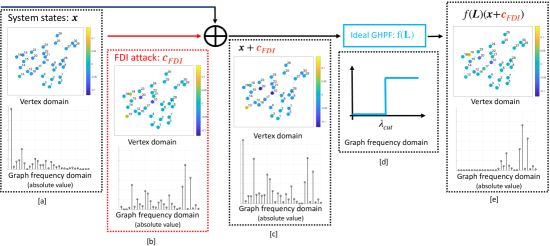
Figure 1: Illustration of GSP-based detection of FDI attacks for the IEEE-30 bus system: the system states are presented in block [a] in both the vertex and graph frequency domains, where it can be seen that the states are smooth, low-frequency graph signals. In block [b], the state attack (${\bf{c}}$ from (15)) is presented, and block [c] presents the contaminated states. It can be seen that, in contrast to the states, the state attack in [b] and the contaminated states in [c] are not smooth graph signals and they have significant energy at the higher graph frequencies. After filtering the contaminated states by the GHPF defined in (11) (shown in block [d]), the filtered signal in block [e] contains only energy at the higher graph frequencies. Consequently, the attack can be discovered by the detector in (18).

II-B GSP smoothness measures

The graph TV of a graph signal ${\bf{s}}$ is defined as [41]

$$TV^{\mathcal{G}}({\bf{s}})\stackrel{{\scriptstyle\triangle}}{{=}}{\bf{s}}^{T}{\bf{L}}{\bf{s}}=\frac{1}{2}\sum_{k=1}^{N}\sum_{n=1}^{N}\omega_{k,n}\big{(}s_{k}-s_{n}\big{)}^{2},$$ (7)

where the last equality is obtained by substituting (1). The TV in (7) is a smoothness measure, which is used to quantify changes w.r.t. the variability that is encoded by the weights of the graph [40]. By substituting (3) and (5) in (7), we obtain

$$TV^{\mathcal{G}}({\bf{s}})=\sum_{k=1}^{N}\lambda_{k}\tilde{s}_{k}^{2}.$$ (8)

According to (8), if ${\bf{s}}$ is smooth, its GFT representation from (5), $\tilde{{\bf{s}}}$, decreases as the graph frequency increases. Thus, low graph TV forces the graph spectrum of the signal to be concentrated in the small eigenvalues region.

The concept of smoothness w.r.t. the graph has been generalized in GSP theory. In GSP theory, the smoothness of the graph signal ${\bf{s}}$ is given by

$$T^{f}({\bf{s}})=\lvert\lvert f({\bf{L}}){\bf{s}}\rvert\rvert^{2},$$ (9)

where $f({\bf{L}})$ is a graph high pass filter (GHPF). The GHPF is a graph filter as defined in (6), where its frequency response, $f(\lambda_{i})$, maintains lower values at the higher graph frequencies. In particular, using the graph frequency response

$$f^{TV}(\lambda_{i})=\sqrt{\lambda_{i}},\leavevmode\nobreak\ i=1,\ldots,N,$$ (10)

we obtain that the smoothness measure in (9) for this case is reduced to the graph TV from (8). Another example is the ideal GHPF, which is defined by the frequency response [60]

$$f^{id}(\lambda_{i})=\begin{cases}0&\lambda_{i}\leq\lambda_{cut}\\ 1&\lambda_{i}>\lambda_{cut}\end{cases}\leavevmode\nobreak\ \leavevmode\nobreak\ \leavevmode\nobreak\ i=1,\ldots,N,$$ (11)

where the cutoff frequency, $\lambda_{cut}$, can be determined based on the application.

II-C Unobservable FDI attacks

A power system is a network of buses (generators or loads) connected by transmission lines that can be represented as an undirected weighted graph, ${\mathcal{G}}({\mathcal{V}},\xi)$, where the set of nodes, $\mathcal{V}$, is the set of $N$ buses, and the edge set, $\xi$, is the set of $P$ transmission lines between these buses. We denote the set of all sensor measurements by $\mathcal{M}$, and the set of transmission lines by $\xi$. We consider the DC model, in which each transmission line, $(k,n)\in\xi$, that connects buses $k$ and $n$ is characterized by a susceptance value $b_{k,n}$, where the branch resistances are neglected [1]. The following noisy and attacked measurement model is considered [1]:

$${\bf{z}}={\bf{H}}{\mbox{\boldmath$\theta$}}+{\bf{a}}+{\boldsymbol{\nu}},$$ (12)

where ${\bf{z}}=[z_{1},\dots,z_{M}]^{T}\in{\mathbb{R}}^{M}$ is the vector of active powers, ${\mbox{\boldmath$\theta$}}=[\theta_{1},\dots,\theta_{N}]^{T}\in{\mathbb{R}}^{N}$ are the state variables (voltage phases), and ${\bf{H}}\in{\mathbb{R}}^{M\times N}$ is the measurements matrix, defined as follows. If row $r$ is associated with the power flow measurement on line $(k,n)$, then

$$H_{\{r,j\}}=\begin{cases}b_{k,n}&j=k\\ -b_{k,n}&j=n\\ 0&\text{otherwise}.\end{cases}$$ (13)

Otherwise, if row $r$ is associated with the power injection measurement in substation $k$, then

$$H_{\{r,j\}}=\begin{cases}\sum_{n\in\mathcal{N}_{k}}b_{k,n}&j=k\\ -b_{k,j}&j\in\mathcal{N}_{k}\\ 0&\text{otherwise},\end{cases}$$ (14)

where $\mathcal{N}_{k}$ is defined in (1). Hence, the measurement matrix is determined by the topology of the network, the susceptance of the transmission lines, and the meter locations. In addition, ${\bf{a}}\in{\mathbb{R}^{M}}$ models an FDI attack and ${\boldsymbol{\nu}}\in{\mathbb{R}}^{M}$ is the measurement noise modeled as a zero-mean Gaussian vector with covariance ${\bf{R}}$.

In the considered setting, any subset of measurements can be regarded as part of the set encompassing active power injections and power flows, as described by the model in (12) with the measurement matrices in (13) and (14). For the sake of simplicity and to ensure that the attack on the states will have an impact on the PSSE approach, in this paper we assume observability of the system. That is, it is assumed that the set of measurements is such that all state variables can be estimated from the available measurements through standard PSSE.

An FDI attack is defined to be unobservable if

$${\bf{a}}={\bf{H}}{\bf{c}},$$ (15)

where the state attack ${\bf{c}}\in{\mathbb{R}}^{N}$ is a nonzero arbitrary vector. The attack in (15) cannot be detected by classical residual-based BDD methods [2]. This can be seen by substituting (15) into (12), which results in

$${\bf{z}}={\bf{H}}({\mbox{\boldmath$\theta$}}+{\bf{c}})+{\boldsymbol{\nu}}.$$ (16)

Thus, the residual calculated with assaulted measurements, ${\bf{z}}-{\bf{H}}(\hat{{\mbox{\boldmath$\theta$}}}+{\bf{c}})$, is the same as it is for normal measurements, ${\bf{z}}_{normal}={\bf{H}}{\mbox{\boldmath$\theta$}}+{\boldsymbol{\nu}}$ (see, e.g., [2, 3]). At the same time, these attacks can be designed to have severe physical [61, 62] and economic consequences [63, 64].

II-D GSP-based FDI attack detection

The problem of detecting FDI attacks based on the DC model in (12) can be formulated as the following hypothesis-testing problem:

$$\begin{cases}\mathcal{H}_{0}:\leavevmode\nobreak\ \hat{{\mbox{\boldmath$\theta$}}}={\mbox{\boldmath$\theta$}}+\bar{{\boldsymbol{\nu}}}\\ \mathcal{H}_{1}:\leavevmode\nobreak\ \hat{{\mbox{\boldmath$\theta$}}}={\mbox{\boldmath$\theta$}}+{\bf{c}}+\bar{{\boldsymbol{\nu}}},\end{cases}$$ (17)

where $\hat{{\mbox{\boldmath$\theta$}}}$ is the PSSE output based on ${\bf{z}}$, and $\bar{{\boldsymbol{\nu}}}$ is the error or noise term associated with the estimation. Recently, it has been shown that GSP-based detectors in the form of [47, 48, 50, 49, 51]:

$$T^{f}(\hat{{\mbox{\boldmath$\theta$}}})\mathop{\gtrless}_{\mathcal{H}_{0}}^{\mathcal{H}_{1}}\gamma,$$ (18)

where $T^{f}(\cdot)$ is defined in (9), are able to solve the hypothesis-testing problem in (17). In this case, the Laplacian matrix of the graph, ${\bf{L}}$, is selected to be the nodal admittance matrix, ${\bf{B}}$, which is a submatrix of ${\bf{H}}$, composed of the rows in ${\bf{H}}$ associated with the power injection measurements described in (14). This selection is applied by setting the edge weights of the graph as $\omega_{k,l}=-b_{k,l}$, where $b_{k,n}<0$ is the susceptance of line $(k,n)\in\xi$. Thus, by by substituting $\omega_{k,l}=-b_{k,l}$ in (1) we obtain the nodal admittance matrix, ${\bf{B}}$.

The GSP-based detector in (18) is based on the assumption that the state vector, $\theta$, is a smooth graph signal w.r.t. to ${\bf{L}}={\bf{B}}$, i.e., that $TV^{G}({\mbox{\boldmath$\theta$}})={\mbox{\boldmath$\theta$}}^{T}{\bf{L}}{\mbox{\boldmath$\theta$}}$ is small compared to other signals in the system, as shown in [50, 48]. In contrast, the state attack vector, ${\bf{c}}$, is a general arbitrary vector that is not smooth w.r.t. the graph. The GSP-based detector in (18) was implemented in [47] with the ideal GHPF defined in (11), and in [50] with the graph TV filter from (10), both with ${\bf{L}}={\bf{B}}$. The detector in (18) can be extended and used for the AC model, as explained in Subsection V-C.

III Graph False Data Injection (GFDI) Attacks

The graph-based detection methodology presented in Section II, which provides the PSSE approach with an additional defense layer against FDI attacks, is illustrated in Fig. 1. In this section, we demonstrate how an adversary could use graph-based information to design an attack that is concentrated in the spectral region of the small eigenvalues and, thus, is more likely to bypass the GSP detection methods (an illustration is provided in Fig. 2). In particular, in Subsection III-A, we formulate the GFDI attack as a constrained optimization problem. Then, in Subsection III-B, we derive the solution for the GFDI attack optimization problem. Finally, some remarks are given in Subsection III-C.

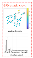
Figure 2: Example of a GFDI attack on the IEEE $30$-bus test case from Fig. 1. It can be seen that the attack energy is located at the lower graph frequencies. Therefore, in contrast to the unobservable FDI attack in Fig. 1[b], when added to the system states, the output will not obtain abnormal energy in the high graph frequencies and, thus, may bypass the GSP-based detectors.

III-A Attack design

The proposed GFDI attack is a special case of unobservable FDI attacks specifically designed to bypass the graph-based detector in (18). The main idea is to design the attack as the output of a smooth fake state signal. Mathematically, let ${\bf{a}}={\bf{H}}{\bf{c}}$ from (15) be the attack vector, and ${\bf{L}}={\bf{B}}$ be the graph Laplacian matrix. Note that ${\bf{B}}$ is the DC nodal admittance matrix, which is a submatrix of ${\bf{H}}$. The state FDI attack, ${\bf{c}}$, is encouraged to be a smooth signal w.r.t. the graph $\mathcal{G}$, i.e., to minimize the graph TV, which according to (7) satisfies

$$TV^{\mathcal{G}}({\bf{c}})={\bf{c}}^{T}{\bf{L}}{\bf{c}}.$$ (19)

Alternatively, as explained in Remark III-C3, the graph TV measure in (19) can be replaced by its generalization in (9), which is used for the GSP-based detection in (18). Simultaneously, the attack should have a substantial impact on the state estimation in order to cause damage. Therefore, in order to make the attack “meaningful”, the adversary further constrains that [11]

$$\lvert\lvert{\bf{c}}\rvert\rvert_{\infty}\geq\tau,$$ (20)

with some positive threshold, $\tau$. In other words, the deviation in the PSSE output in (17) caused by at least one element in ${\bf{c}}$ should be larger than the threshold $\tau$.

In addition, the attack design considers practical limitations. First, as in other FDI attacks (see, e.g., [2, 65]), the attack should be sparse. Specifically, similar to previous works (see, e.g., [21, 66, 22, 67, 11, 68]), the sparsity constraint is applied directly on the state attack vector ${\bf{c}}$, i.e., the number of the manipulated state variables is considered to be small. For a sparsity parameter $k\in\mathbb{R}_{+}$, the attack is constrained by

$$\lvert\lvert{\bf{c}}\rvert\rvert_{0}\leq k,$$ (21)

where $\lvert\lvert\cdot\rvert\rvert_{0}$ is the $\ell_{0}$ semi-norm defined as the number of nonzero elements of its argument.

Simulations performed in [2] show that the assumption in (21) stems directly from the commonly-used sparsity restriction on the number of manipulated meters, which states that the attack vector, ${\bf{a}}$, is sparse.

Finally, it is assumed that certain security constraints are imposed by the system designer. Specifically, we assume that a set of indices corresponding to the measurement set is protected. The measurement constraint for the attacker can be expressed as

$${\bf{H}}^{\mathcal{S}}{\bf{c}}={\bf{0}}.$$ (22)

In the above, we denote by ${\bf{H}}^{\mathcal{S}}$ the matrix formed by the $\lvert\mathcal{S}\rvert$ rows of ${\bf{H}}$ indicated by the indices in $\mathcal{S}$. The constraint in (22) implies that the measurements in the set $\mathcal{S}$ do not contribute to the attack vector ${\bf{a}}$ in (15).

To conclude, the attack has two main conflicting goals: to be less detectable by GSP tools (as described in (19)), while causing a significant impact on the power system (as described in (20)). These two goals should be achieved while adhering to the physical constraints on the possible attacked locations: a quantitative constraint (described in (21)) and a qualitative constraint on the specific sensors (described in (22)). This can be formalized by the following optimization problem:

$$\underset{{\bf{c}}\in\mathbb{R}^{N}}{\min}\leavevmode\nobreak\ {\bf{c}}^{T}{\bf{L}}{\bf{c}}$$ (23)

$$\text{s.t.}\begin{cases}\lvert\lvert{\bf{c}}\rvert\rvert_{\infty}\geq\tau\\ \lvert\lvert{\bf{c}}\rvert\rvert_{0}\leq k\\ {\bf{H}}^{\mathcal{S}}{\bf{c}}={\bf{0}}.\end{cases}$$

Roughly speaking, the proposed GFDI attack in (23) is the smoothest attack possible that ensures sufficient damage and considers practical limitations of sparsity and restricted measurements. It can be seen that without the extra constraint in (20), a trivial optimal solution to the optimization in (23) is ${\bf{c}}={\bf{0}}$, which means that the attacker does not attack the system.

In the following, we show the necessity of the constraints from the GFDI optimization problem in (23).

1. No impact: The impact parameter $\tau$ must satisfy $\tau>0$. This is since otherwise, i.e., if $\tau=0$, then the solution of (23) is ${\bf{c}}={\bf{0}}$, which implies zero-attack (${\bf{a}}={\bf{0}}$).

2. Sparsity: The sparsity parameter $k$ must satisfy $k<N$. Otherwise, for $k=N$ the solution of (23) is in the linear space spanned by the first eigenvector of the Laplacian matrix, i.e., ${\bf{c}}\in\mathrm{span}(\mathbf{1})$. This can be seen from the fact that the smallest eigenvalue of the Laplacian is $0$, which guarantees that ${\bf{c}}^{T}{\bf{L}}{\bf{c}}=0$. This is the lowest value of TV possible, since ${\bf{L}}$ is a positive semidefinite matrix. Moreover, it can be verified from (13) and (14) that a solution ${\bf{c}}\in\mathrm{span}(\mathbf{1})$ results in an attack vector ${\bf{H}}{\bf{c}}={\bf{0}}$. Thus, ${\bf{c}}\in\mathrm{span}(\mathbf{1})$ is a feasible solution since it satisfies ${\bf{H}}^{\mathcal{S}}{\bf{c}}={\bf{0}}$. However, in this case, the system is not really attacked in the sense of ${\bf{a}}$, and thus, this is a degenerative case. It should also be noted that in the case where the constraint $\lvert\lvert{\bf{c}}\rvert\rvert_{0}\leq k$ is replaced with $\lvert\lvert{\bf{a}}\rvert\rvert_{0}\leq k$, the solution is bound to satisfy ${\bf{c}}\in\mathrm{span}(\mathbf{1})$ such that it has no impact on the actual states. Thus, in the considered setting, $\lvert\lvert{\bf{c}}\rvert\rvert_{0}\leq k$ is the appropriate sparsity constraint.

3. No availability: A feasible solution may not exist when the secured set $\mathcal{S}$ includes a substantial number of sensors. In the extreme case where $\mathcal{S}$ contains all the system sensors, it is obvious that an FDI attack is infeasible. However, if an unobservable FDI attack that satisfies the sparsity and impact restriction in (23) is available for a selected set $\mathcal{S}$, then a GFDI attack is available as well, i.e., (23) has a solution.

III-B GFDI attack implementation

The optimization problem in (23) is composed of a quadratic objective function, ${\bf{c}}^{T}{\bf{L}}{\bf{c}}$, with: 1) a concave inequality constraint, $\|{\bf{c}}\|_{\infty}\geq\tau$, since the $\ell_{\infty}$-norm is a convex function [58]; 2) a non-convex sparsity constraint, $\lvert\lvert{\bf{c}}\rvert\rvert_{0}$; and 3) a linear constraint, ${\bf{H}}^{\mathcal{S}}{\bf{c}}={\bf{0}}$. Hence, (23) is a non-convex optimization problem. In this subsection, we derive a solution for this problem.

The following theorem suggests an equivalent optimization problem for the GFDI attack optimization problem in (23).

Theorem 1.

The solution of the GFDI attack optimization problem in (23), $\hat{{\bf{c}}}$, can be obtained by solving the following series of optimization problems:

$$\underset{i=\{1,\ldots,N\}}{\min}\underset{{\bf{c}}\in\mathbb{R}^{N}}{\min}\leavevmode\nobreak\ {\bf{c}}^{T}{\bf{L}}{\bf{c}}$$ (24)

$$\text{s.t.}\begin{cases}c_{i}=\tau\\ \lvert\lvert{\bf{c}}\rvert\rvert_{0}\leq k\\ {\bf{H}}^{\mathcal{S}}{\bf{c}}={\bf{0}}.\end{cases}$$

Proof.

The proof is given in Appendix A. ∎

It can be seen that in the inner minimization in (24), the $\ell_{\infty}$ inequality constraint from (23) is replaced with the $i$th linear constraint, $c_{i}=\tau$. In addition, it can be seen that the inner optimization problem in (24) is composed of a quadratic objective function with sparsity and linear constraints. Hence, the major issue for the attacker is that solving optimization problems with $\ell_{0}$ constraints is, in general, NP-hard. Following standard sparse recovery techniques [69], the $\ell_{0}$-norm can be replaced by its $\ell_{1}$-norm relaxation version that promotes sparsity. Thus, the attacker can solve the following convex relaxation:

$$\underset{{\bf{c}}\in\mathbb{R}^{N}}{\min}\leavevmode\nobreak\ {\bf{c}}^{T}{\bf{L}}{\bf{c}}$$ (25)

$$\text{s.t.}\begin{cases}c_{i}=\tau\\ \lvert\lvert{\bf{c}}\rvert\rvert_{1}\leq k\\ {\bf{H}}^{\mathcal{S}}{\bf{c}}={\bf{0}}.\end{cases}$$

That is, instead of solving (23), the adversary should solve a series of $N$ convex optimization problems obtained by setting $i=\{1,\ldots,N\}$ in (25). The final step comprises selecting the minimum from the $N$ solutions.

By introducing the nonnegative vector variables ${\bf{u}}\geq{\bf{0}}$ and ${\bf{v}}\geq{\bf{0}}$, where the vector inequality indicates elementwise inequalities, the problem in (25) can be formulated as a quadratic programming problem, as follows:

$$\underset{{\bf{c}}\in\mathbb{R}^{N}}{\min}\leavevmode\nobreak\ {\bf{c}}^{T}{\bf{L}}{\bf{c}}$$ (26)

$$\text{s.t.}\begin{cases}c_{i}=\tau\\ {\bf{H}}^{\mathcal{S}}{\bf{c}}={\bf{0}}\\ {\bf{c}}={\bf{u}}-{\bf{v}}\\ {\bf{1}}^{T}({\bf{u}}+{\bf{v}})\leq k\\ {\bf{u}}\geq{\bf{0}},{\bf{v}}\geq{\bf{0}},\end{cases}$$

where ${\bf{1}}$ is the all-one vector. The quadratic programming problem in (26) can be efficiently solved using interior point methods[58], e.g., using the Matlab function quadprog.

After solving (26), if a feasible solution is found, then case $i$ is added to the set of possible solutions, $\mathcal{I}$, and the solution is denoted by ${\bf{c}}^{*,i}$. In order for the solution ${\bf{c}}^{*,i}$ to be at most $k$-sparse, as required by the original constraints of the problem in (24), we apply a hard-thresholding step and only keep the $k$ largest (in the sense of the absolute value of the magnitudes) components of ${\bf{c}}^{*,i}$, while zeroing out the remaining entries. On the other hand, if a feasible solution is not available, then case $i$ is not included in $\mathcal{I}$.

After solving (26) for $i=1,\ldots,N$, we determine the optimal position to attack the system by choosing the optimal solution among the candidates in $\mathcal{I}$:

$$\hat{i}=\arg\underset{i\in\mathcal{I}}{\min}\leavevmode\nobreak\ ({\bf{c}}^{*,i})^{T}{\bf{L}}{\bf{c}}^{*,i}.$$ (27)

Next, we calculate the optimal attack by setting $\hat{{\bf{a}}}={\bf{H}}\hat{{\bf{c}}}$, where $\hat{{\bf{c}}}={\bf{c}}^{*,\hat{i}}$ and $\hat{i}$ is given in (27). However, due to the thresholding step applied after solving (26), there is no guarantee that the resulting $\hat{{\bf{c}}}$ maintains the constraint on the secured sensors from (26), i.e., there is no guarantee that $\hat{{\bf{a}}}_{\mathcal{S}}={\bf{H}}^{\mathcal{S}}\hat{{\bf{c}}}={\bf{0}}$. Therefore, in order for the final solution $\hat{{\bf{c}}}$ to be a feasible solution, we set the elements in $\hat{{\bf{a}}}$ that correspond to the set $\mathcal{S}$ to zero, i.e., we set

$$\hat{{\bf{a}}}_{\mathcal{S}}={\bf{0}}.$$ (28)

Algorithm 1 GFDI attack creation

0:    ${\bf{L}}$, $k$, $\tau$, $\mathcal{S}$, ${\bf{H}}$

0:  $\hat{i}$, $\hat{{\bf{c}}}$, and $\hat{{\bf{a}}}$

1:  Initialize $\mathcal{I}=\emptyset$

2:  for $i\in\{1,\ldots,N\}$ do

3:     solve (26) (e.g., by Matlab quadprog)

4:     if a feasible solution, ${\bf{c}}^{*,i}$, is found  then

5:        update $\mathcal{I}=\mathcal{I}\cup i$

6:        set $c^{*,i}_{m}=0$ for $m>k$ and $\lvert c^{*,i}_{j_{1}}\rvert\geq\ldots\geq\lvert c^{*,i}_{j_{N}}\rvert$

7:     else

8:        go to line 2

9:     end if

10:  end for

11:  if  $\mathcal{I}=\emptyset$ then

12:     return  “no feasible solution”

13:  else

14:     compute: $\hat{i}=\arg\underset{i\in\mathcal{I}}{\min}\leavevmode\nobreak\ ({\bf{c}}^{*,i})^{T}{\bf{L}}{\bf{c}}^{*,i}$

15:     set $\hat{{\bf{c}}}={\bf{c}}^{*,{\hat{i}}}$ and $\hat{{\bf{a}}}={\bf{H}}\hat{{\bf{c}}}$

16:     update $\hat{{\bf{a}}}_{\mathcal{S}}={\bf{0}}$

17:     return  $\hat{i}$, $\hat{{\bf{c}}}$, and $\hat{{\bf{a}}}$

18:  end if

III-C Remarks

III-C1 Attack Unobservability

Due to Step $16$ in Algorithm 1, the attack $\hat{{\bf{a}}}$ can be viewed as the following superposition:

$$\hat{{\bf{a}}}={\bf{H}}\hat{{\bf{c}}}+\tilde{{\bf{a}}},$$ (29)

where the vector $\tilde{{\bf{a}}}$ is such that $\tilde{{\bf{a}}}_{S}=\hat{{\bf{a}}}^{S}-{\bf{H}}^{\mathcal{S}}\hat{{\bf{c}}}$ and $\tilde{{\bf{a}}}_{\{\mathcal{M}\setminus\mathcal{S}\}}={\bf{0}}$. Consequently, the proposed attack cannot be considered as a pure unobservable attack in the sense of (15). Nonetheless, we expect that $\|\tilde{{\bf{a}}}\|\leq\epsilon$, where $\epsilon$ is a significantly low value. This implies that

$$\|\hat{{\bf{a}}}-{\bf{H}}\hat{{\bf{c}}}\|_{2}^{2}\leq\epsilon.$$

Hence, this attack can be referred to as a generalized unobservable FDI attack (see Section 4.1. in [2]) and is still expected to be undetected by classical residual-based BDD methods if a certain degree of noise is present.

III-C2 Known topology

An assumption behind the GFDI attack design in (23) is that ${\bf{L}}$ is known. In other words, it is required that the adversary knows the power system network configuration. The same assumption is required for generating the unobservable FDI attack in (15) [2, 65]. The assumption that ${\bf{H}}$ (and consequently its submatrix ${\bf{B}}$) is known or can be estimated from historical data [7, 8, 9, 10], gives the adversary more power than usually is possible in reality. We note that this is a well-adopted practice in the cyber-security community, which increases the system’s resilience.

III-C3 Generalization to graph filters

The objective function of the GFDI optimization problem in (23) can be generalized by replacing the graph TV measure in (19) with a general GSP-based smoothness measure in (18), which measures the energy of the estimated PSSE after it has been filtered by a selected GHPF. In this case, the quadratic programming optimization in (26) is modified by replacing the cost function with $f({\bf{c}})=\|f({\bf{L}}){\bf{c}}\|^{2}$, where $f({\bf{L}})$ is a general graph filter as defined in (6). In particular, we can obtain the following two special cases: 1) if the GHPF is selected as (7), then we obtain the same result provided by the graph TV measure, described above and summarized in Algorithm 1; and 2) if the GHPF is selected as (11), then the attack obtained will be a graph low pass signal with energy located only in the $k$ smallest graph frequencies, as conceptualized in [51]. Thus, the proposed approach also suggests an implementation for the theoretical idea in [51].

III-C4 Applicability of the GFDI attack for the AC model

The nonlinear AC provides a more accurate representation of the power flow equations than the DC model presented in Section II [65]. As described in Section II, constructing an unobservable FDI attack for the DC model required knowledge of the system configuration represented by ${\bf{H}}$. In contrast, constructing an unobservable FDI attack for the AC model requires knowledge of both ${\bf{H}}$ and the current state of the system [65], which is often considered unrealistic. However, since the DC model is a linearization of the AC model, a DC-based attack could work approximately on the AC model [65]. We show the applicability of our attack design on both the DC and the AC models in the simulation study in Section V.

IV Strategic protection of the power network

In addition to GSP-based detection, the operator may install additional security hardware to disable access to selected measurements for an adversary. In this section our goal is to demonstrate how to harvest the graph-based knowledge, used for the design of the GFDI attack in Section III, in order to strategically select the protected measurements. Specifically, we aim to identify the minimal set of measurements required to prevent the possibility of a GFDI attack. This section is organized as follows. In Subsection IV-A we discuss the protection scheme design. Then, in Subsection IV-B we provide a practical implementation. We conclude with remarks in Subsection IV-C.

IV-A Protection scheme design

In practice, our protection scheme identifies a minimal set of state variables (denoted by $\mathcal{D}$), such that if secured (not manipulated), it would disable the possibility of generating a GFDI attack. After identifying $\mathcal{D}$, we can then deduce the set of secured measurements (denoted by $\mathcal{S}$) in one of the following two ways: 1) the set $\mathcal{S}$ is composed from the power measurements positioned in the buses in set $\mathcal{D}$ (power injections) and in the lines entering these buses (power flows); and 2) the set $\mathcal{S}$ is composed from PMU measurements installed at the same locations as in set $\mathcal{D}$. In our implementation, we adopt the first option.

The proposed protection scheme is formulated by the following heuristic optimization problem:

$$\hat{\mathcal{D}}=\arg\underset{\mathcal{D}\subseteq\mathcal{V}}{\min}\leavevmode\nobreak\ \lvert\mathcal{D}\rvert\leavevmode\nobreak\ s.t.\leavevmode\nobreak\ (\hat{{\bf{c}}})^{T}{\bf{L}}\hat{{\bf{c}}}>\delta,$$ (30)

where $\hat{{\bf{c}}}$ is the output of the GFDI attack optimization problem in (23), which is implemented by Algorithm 1. Thus, the problem in (30) searches for the set $\mathcal{D}$ with the minimal cardinality, for which the graph TV of the optimal GFDI solution exceeds a user-defined threshold $\delta>0$, and therefore, can be detected by GSP methods. Selecting a minimal set of secured state variables enables the operator to reduce the installation cost of security hardware.

The underlying assumption behind the strategic protection design in (30) is its effectiveness against the proposed GFDI attack, along with its capability to provide a defense against various potential smooth attack vectors that may not be the optimal GFDI attack. Furthermore, this framework can be extended to other GSP-based attacks described in Remark III-C3 by using the generalization to other GHPFs. Future research is needed to identify an optimal protection strategy that can defend the system against a broad spectrum of smooth attacks.

IV-B Implementation

The problem in (30) is a combinatorial optimization problem with a non-submodular objective function. Thus, the number of possible instances for $\mathcal{D}$ grows exponentially with the system size, $N$. Moreover, it can be seen that, for each instance, the objective function requires implementing Algorithm 1. Thus, (30) will suffer from high computational complexity due to the exhaustive search and is not practical for large networks. Therefore, we propose a low-complexity greedy algorithm for selecting the state variables to be protected, as described in Algorithm 2.

We start with an empty set, $\mathcal{D}=\emptyset$, and iteratively compose $\mathcal{D}$ as follows. In each iterative step, the GFDI problem in (24) is first solved by Algorithm 1, taking into account the set $\mathcal{S}$ composed from the power measurements positioned at the buses in the current set $\mathcal{D}$ (power injections) and in the lines entering these buses (power flows). Then, the state variable at position $i$, where the attack obtains the maximal value $\tau$, is added to the secured state variable set $\mathcal{D}$.

Algorithm 2 Protection scheme

0:  ${\bf{L}}$, $k$, $\tau$, $\delta$

0:  $\mathcal{D}$

1:  Initialize: $\mathcal{D}=\emptyset$

2:  repeat

3:     derive $\mathcal{S}$ from $\mathcal{D}$ by including power injections in the buses in $\mathcal{D}$ and power flows entering the same buses

4:      get $\hat{i}$ and $\hat{{\bf{c}}}$ from GFDI Algorithm

5:     add $\hat{i}$ to $\mathcal{D}$

6:  until $(\hat{{\bf{c}}})^{T}{\bf{L}}\hat{{\bf{c}}}>\delta$

7:  return  $\mathcal{D}$

IV-C Remarks

IV-C1 Generalization to graph filters

If the GFDI optimization problem is realized with a general graph filter as explained in Remark $2)$ in Subsection III-C, then the constraint in (30) should be replaced accordingly. The following is conducted by replacing the graph TV measure in (30) with $\|f({\bf{L}}){\bf{c}}\|^{2}$, which is obtained by substituting ${\bf{s}}=\hat{\bf{c}}$ in (9). In this case, row $4$ of Algorithm 2 calls Algorithm 1 with the changes discussed in Remark $2)$ in Subsection III-C.

IV-C2 Comparison to previous protection schemes

The proposed protection scheme differs from previous designs in that it does not aim to prevent the adversary from launching an FDI attack. Rather, it seeks to eliminate the possibility of an attack with low graph TV. Consequently, the proposed designs forces the GFDI output to be a non-smooth attack, which, with high probability, would be detected by a GSP-based detector. As a result, there are two minor drawbacks and one significant advantage. The first drawback is that a GSP-based detector must be installed in the system control center. However, since these detectors are software-based, they can be implemented easily. The second drawback is that if an attack is detected, the system still operates with unreliable measurements, which is currently a common limitation of detection policies. On the other hand, the relaxation provided by enabling a GFDI attack instead of no FDI attack at all significantly reduces the number of secured measurements required, as demonstrated in the simulation study (see Fig. 5).

V Simulation study

This section demonstrates the performance of the proposed GFDI attack and GSP-based protection policy by numerical simulations. The simulations are conducted on the IEEE-$57$ and IEEE-$118$ bus test cases, where the topology matrix and measurement data are extracted using the Matpower toolbox for Matlab [70]. In Subsection V-A, we describe the FDI attack construction methods, and protection policies used as reference. The simulation setup is then provided in Subsection V-B. Next, we present the analysis conducted for the GFDI attack in Subsection V-C and for the GSP-based protection policy in Subsection V-D.

V-A Methods

V-A1 FDI attack constructions

The GFDI attack (denoted as GFDI) implemented by Algorithm 1 is compared to previous unobservable FDI attacks. Considering that an unobservable FDI attacks satisfies ${\bf{a}}={\bf{H}}{\bf{c}}$, where ${\bf{H}}$ is a known parameter, the attack can be equivalently defined using the state attack ${\bf{c}}$. The previous designs include the following:

1. Random unobservable FDI attack [2] (denoted as rand): This attack is constructed by: 1) selecting $k$ elements randomly for the support of the state attack, ${\bf{c}}$; and 2) assigning random values at these index locations according to the Gaussian distribution, $\mathcal{N}(0,1)$.

2. Random unobservable FDI attack with GFDI support (denoted as rand+GFDI): The state attack support is the one obtained from the GFDI solution in Algorithm 1, where random values are assigned to the selected indices following the Gaussian distribution, $\mathcal{N}(0,1)$.

3. The sparsest unobservable FDI attack with the lowest graph TV (denoted as sparse-low): The attack defined by the linear programming problem in Equation (14) in [11] solved using the Matlab function linprog. If there is more than one solution, the one with the lowest graph TV is chosen as the attack.

4. The sparsest unobservable FDI attack with average graph TV (denoted as sparse-avg): The attack defined by the linear programming problem in Equation (14) in [11] solved using the Matlab function linprog. In this case, if there is more than one solution, the one closest to the average graph TV is chosen.

The attacks are scaled to satisfy $\lvert\lvert{\bf{c}}\rvert\rvert_{\infty}=\tau$.

V-A2 Protection policies

The proposed GSP-based protection policy, suggested in Section IV in the presence of a GFDI attack, is compared with the following protection policies:

1. Random-based protection policy, where the elements in $\mathcal{D}$ are selected randomly.

2. Sparsest-based protection policy, where the elements in $\mathcal{D}$ are selected to increase the number of nonzero elements in ${\bf{c}}$ required for a feasible unobservable FDI attack described by Equation (14) in [11]. The policy is defined in Algorithm $3$ in [11].

V-B Simulation setup

The simulations were conducted on the IEEE-$57$ and IEEE-$118$ bus test cases. Detection thresholds were computed from simulated historical data obtained by $10,000$ off-line simulations of (12) under the null hypothesis. All numerical results were obtained using $10,000$ Monte Carlo simulations. The FDI attacks in both settings are modeled by the GFDI attack and Attacks A.1-A.4.

V-B1 DC model

For the DC model, the measurements are computed using (12). The state vector, ${\bf{x}}$, is assumed to be a smooth graph signal that has a low graph TV, as defined in (7), and is modeled as follows [71, 72]. In particular, we first set $\tilde{x}_{1}=0$ and generate

$$\tilde{{\bf{x}}}_{2:end}\sim\mathcal{N}({\bf{0}},\beta\boldsymbol{\Lambda}^{-1}_{2:end,2:end}),$$ (31)

where $\beta$ is a smoothness level selected as $\beta=0.05$. Then, we use the IGFT defined below (5) to obtain ${\bf{x}}={\bf{U}}\tilde{{\bf{x}}}$.

The measurement noise is modeled as a zero-mean Gaussian noise with variance $0.001{\bf{I}}$. In addition, one of the additive attacks presented in Subsection V-A is added to the measurements.

V-B2 AC model

For the AC model, the measurements are modeled by

$${\bf{z}}_{AC}={\bf{v}}({\bf{Y}}{\bf{v}})^{*}+{\bf{a}}+{\bf{e}}_{c},$$ (32)

where ${\bf{v}}$ are the complex voltages located at the system buses and ${\bf{Y}}$ is the admittance matrix. The voltage phases are generated according to (31). The voltage magnitudes, which are assumed to be close to $1$, are generated according to

$$\lvert{\bf{v}}\rvert\overset{i.i.d}{\sim}\mathcal{N}(1,0.01).$$ (33)

The matrix ${\bf{Y}}$ follows the structure in (1), but, in this case, the weights are complex [47]. As discussed in Subsection III-C, the same attack used on the DC model is also used on the AC model. Hence, one of the attacks in Subsection V-A is added to the measurements. The measurement noise, ${\bf{e}}_{c}$, is modeled as a circularly-symmetric complex Gaussian vector with zero-mean and a variance of $0.001$, i.e., ${\bf{e}}_{c}\sim\mathcal{CN}({\bf{0}},0.001{\bf{I}})$.

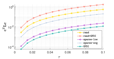
(a) Graph TV

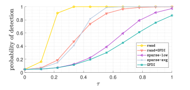
(b) Probability of detection

Figure 3: The GFDI attack is compared to Attacks A.1-A.4. In (a) and (b), the graph TV of the attacks and the probability of detection, respectively, are presented versus $\tau$. The curves of the probability of detection are generated w.r.t. to the GTV-GHPF detector for the DC model.

V-C GFDI attack analysis

Figure 3.(a) presents the graph TV of the attacks as a function of the attack impact $\lvert\lvert{\bf{c}}\rvert\rvert_{\infty}=\tau$ (see (19)) for $k=5$ and $\mathcal{S}=\emptyset$ over the IEEE-$57$ bus test case. It can be seen that the GFDI attack ($\hat{{\bf{c}}}$ from Algorithm 1) has the lowest graph TV, while the other attacks generally demonstrate a rapid increase in the graph TV as $\tau$ increases. These results can be interpreted as an indication of the vulnerability of the different attacks to the GSP-based detectors in the form of (18). For this scenario, there is only one nonzero element in Attacks A.3-A.4. Thus, A.3 is the attack with the lowest TV from all FDI attacks limited to manipulate only one state variable. It can be seen that enabling the adversary to manipulate more than one element, as performed in the GFDI attack, results in better detection performance.

Figure 3.(b) presents the probability of detection as a function of the attack impact, $\lvert\lvert{\bf{c}}\rvert\rvert_{\infty}=\tau$, for $k=5$ and $\mathcal{S}=\emptyset$ over the IEEE-$57$ bus test case. The detection is conducted by the GTV-GHPF detector, which is obtained by applying (9) with the GHPF in (10) and with a false alarm probability of $0.05\%$. The results show that the probability of detection increases as $\tau$ increases, as expected. Comparing the results in Fig. 3.(b) with those in Fig. 3.(a) confirms the assumption that smooth attacks are harder to detect by GSP-based detectors. As a result, the GFDI ($\hat{{\bf{a}}}$ from Algorithm 1) is the attack that is the hardest to detect. The sparse-low attack that is suggested in this paper takes the attack with the lowest graph TV from all the possible results provided by solving (14) in [11], and provides the closes probability of detection to the proposed GFDI attack. However, it is important to note that the authors of [11], who introduced the sparsest attack, did not discuss the influence of graph TV on detection. Thus, selecting the attack with the lowest graph TV, i.e., the sparse-low attack, can be seen as an additional contribution of this paper. Compared to the GFDI attack, the random FDI attacks and the sparse-avg attack are easily detected.

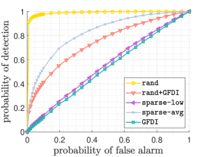
(a) DC model

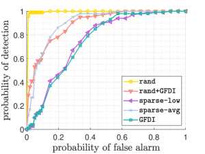
(b) AC model

Figure 4: The GFDI attack is compared to Attacks A.1-A.4. In (a) and (b), the ROC curves of the attacks are generated w.r.t. to the GTV-GHPF detector for the DC model and the AC model, respectively.

Figure 4.(a) presents the ROC curves (probability of detection versus probability of false alarm) of the GTV-GHPF detector for the different unobservable FDI attacks under the DC simulation setup with $\tau=0.2$, $k=5$, and $\mathcal{S}=\emptyset$ over the IEEE-$57$ bus test case. It can be seen that the GFDI attack ($\hat{{\bf{a}}}$ from Algorithm 1) is the hardest to detect, while it performs slightly better than the sparse-low attack Figure. 4.(b) presents the ROC curves of the GTV-GHPF detector for the different unobservable FDI attacks under the AC simulation setup with $\tau=0.07$ and $k=5$ over the IEEE-$30$ bus test case. It can be seen that the relationship between attack designs in Fig. 4.(b), where attacks with low graph TV are less likely to be detected by the GSP-based detectors, is similar to those in Fig. 4.(a). An extension of the GTV-GFHP to the AC is provided as follows.

• GTV-GHPF: Based on our results in [50, 49], an alert to an attack is provided if the GSP-based detector in (18) when using the GTV-GHPF in (10) indicates an attack for at least one of the following cases: 1) ${\bf{L}}={\bf{B}}$, ${\bf{y}}=\Re\{\hat{\boldsymbol{\theta}}\}$, where $\hat{\boldsymbol{\theta}}$ are the phases of $\hat{{\bf{v}}}$; and/or 2) ${\bf{L}}={\bf{B}}$, ${\bf{y}}=\lvert\hat{\bf{v}}\rvert-\boldsymbol{1}\lvert\hat{v}_{1}\rvert$.

Similar detection results to those presented in Figs. 3.(b), 4.(a), and 4.(b) were found when using the Ideal-GHPF detector, obtained by substituting (11) in (18). In addition, we verified that the BDD detector cannot detect any of the attacks, since they are all unobservable. Extensions of the Ideal-GFHP and BDD detectors for the AC model can be obtained as follows.

• Ideal-GHPF: Attack alert is provided if the GSP-based detector in (18) when using the ideal GHPF in (11) indicates an attack for at least one of the following cases: 1) ${\bf{L}}=\Re\{{\bf{Y}}\}$, ${\bf{y}}=\Re\{\hat{{\bf{v}}}\}$; 2) ${\bf{L}}=\Re\{{\bf{Y}}\}$, ${\bf{y}}=\Im\{\hat{{\bf{v}}}\}$; 3) ${\bf{L}}=-\Im\{{\bf{Y}}\}$, ${\bf{y}}=\Re\{\hat{{\bf{v}}}\}$; and/or 4) ${\bf{L}}=-\Im\{{\bf{Y}}\}$, ${\bf{y}}=\Im\{\hat{{\bf{v}}}\}$. The vector $\hat{{\bf{v}}}$ is the AC PSSE output.

• BDD: The BDD detector for the AC model ${\lvert\lvert{\bf{z}}_{AC}-\hat{{\bf{v}}}({\bf{Y}}\hat{{\bf{v}}})^{*}\rvert\rvert_{2}^{2}\gtrless_{\mathcal{H}_{0}}^{\mathcal{H}_{1}}}$, where $\hat{{\bf{v}}}$ is the AC PSSE output.

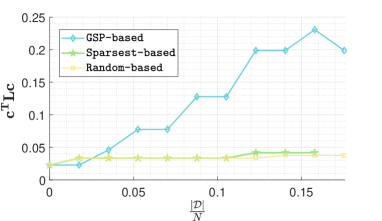
(a) Protection policy analysis (IEEE-57)

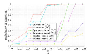
(b) Protection impact on detection (IEEE-57)

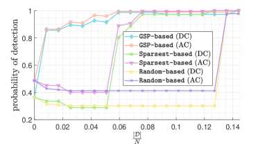
(c) Protection impact on detection (IEEE-118)

Figure 5: The GSP-based protection policy is compared to Policies P.1-P.2. The IEEE-$57$ bus test case is observed in (a) and (b), where in (a), the GFDI attack graph TV and in (b), the probability of detecting the GFDI attack by the GTV-detector, are presented versus the ratio of the secured state variables out of the total number of states, $\frac{\lvert\mathcal{D}\rvert}{N}$. In (c), the case in (b) is examined over the IEEE-$118$ bus test case.

V-D GSP-based protection policy analysis

Figure 5 illustrates the influence of securing system state variables, according to the different protection policies, on the GFDI attack. In Fig. 5.(a) the graph TV of the GFDI attack ($\hat{{\bf{c}}}$ from Algorithm 1) is presented versus the ratio between the secured state variables and the total number of states for the IEEE-$57$ bus test case with $\tau=0.6$ and $k=3$. The results indicate that using a GSP-based policy leads to an immediate increase in graph TV as the number of protected state variables increases. In comparison, Policies P.1-P.2 have only a minor effect on the graph TV. In addition, it is important to mention that when at least $0.175\%$ of the state variables are secured, Policy P.2 prevents the generation of the smooth attack. Figure 5.(b) examines the probability of detecting the GFDI attack by the GTV-GHPF detector, with a false alarm probability of $0.05\%$, for the IEEE-$57$ bus test case under both the DC and AC models. For the simulations conducted on the DC and AC models, we used $(\tau,k)=(0.6,3)$ and $(\tau,k)=(0.25,3)$, respectively. It can be seen that protecting a low percentage of state variables according to the locations provided by a GSP-based protection policy can significantly enhance the detection probability. This is also true in Fig. 5.(c), which examines the probability of detecting the GFDI attack by the GTV-GHPF detector, with a false alarm probability of $0.05\%$, for the IEEE-$118$ bus test case under both the DC and AC models. For the simulations conducted under the DC and AC models, we used $(\tau,k)=(0.55,5)$ and $(\tau,k)=(0.28,5)$, respectively. It can be seen in Figs. 5.(b) and 5.(c) that protecting state variables according to the locations provided by a sparse-based protection policy also enhances the detection probability. However, this policy necessitates securing a significantly higher proportion of state variables. Moreover, it should be noted that the sparsest-based policy was created to prevent the possibility of an attack being generated, which requires, in general, securing at least $30\%$ of the state variables. Finally, it can be seen that protecting state variables according to the locations provided by a random-based protection policy does not promote enhanced detection probability unless a large portion of state variables is secured. Moreover, similar behavior is witnessed for both the DC and AC models, where for both models, the proposed protection scheme significantly enhances the detection probability by protecting only a small percentage of state variables.

VI Conclusions

We introduce a new, GSP-based, defensive approach against FDI attacks in power systems. First, from the adversary’s point of view, we present a new unobservable FDI attack, the GFDI attack, that utilizes the graph properties of the states to bypass the recently developed GSP-based detectors. Then, from the perspective of the system operator, we present countermeasures against the GFDI attacks. The proposed protection scheme aims to select a minimal set of sensors to prevent the success of GFDI attacks by forcing the attack to have a high graph TV and, thus, enabling its detection by advanced GSP tools. This approach requires a smaller set of secured states than existing designs, which translates to a lower construction cost and a shorter installation time for new hardware. The proposed GFDI attack design and protection scheme are applicable for both DC and AC models. Our numerical simulations show that existing detection methods have a significantly lower detection probability for the proposed GFDI attack compared to previous attack designs, indicating the significant threat posed by the GFDI attack to power systems. Moreover, the simulations demonstrate that our proposed GSP-based protection scheme requires a smaller set of secured sensors compared to existing designs, resulting in lower construction costs and shorter installation times. Therefore, our approach provides a new and cost-effective solution for enhancing the resilience of power systems against FDI attacks. Future research should include a practical investigation of the GSP-based detectors, attacks, and protection schemes under various real-world settings. Other research directions involve extending the GFDI attack design and the proposed protection scheme to partially observable systems, as well as optimizing the protection scheme. In addition, the proposed approach, including the attack and protection design, could be extended to general sensor networks that are based on GSP data tasks.

Appendix A Proof for Theorem 1

Let ${\bf{c}}^{*}$ and ${\bf{c}}^{**}$ be the optimal solutions of (23) and (24), respectively. In the following, we first show that $({\bf{c}}^{**})^{T}{\bf{L}}{\bf{c}}^{**}\leq({\bf{c}}^{*})^{T}{\bf{L}}{\bf{c}}^{*}$ and then that ${\bf{c}}^{**}$ is in the feasible set of (23). If both requirements are met, then ${\bf{c}}^{**}$ is a feasible solution in the minimization problem (23) with a cost function smaller than the cost function associated with the optimal solution, ${\bf{c}}^{*}$. Therefore, ${\bf{c}}^{**}$ is the optimal solution of (23), i.e., ${\bf{c}}^{*}={\bf{c}}^{**}$.

Without loss of generality, let the index $j$ be such that $\lvert\lvert{\bf{c}}^{*}\rvert\rvert_{\infty}=\lvert c^{*}_{j}\rvert$ and define $\bar{{\bf{c}}}^{*}={\text{sign}}(c^{*}_{j})\frac{\lvert c_{j}^{*}\rvert}{\tau}{\bf{c}}^{*}$, where ${\text{sign}}(\cdot)$ denotes the sign function, which assigns $1$ to positive argument and $-1$ for negative ones. As a result, we obtain that

$$(\bar{{\bf{c}}}^{*})^{T}{\bf{L}}\bar{{\bf{c}}}^{*}=(\tau/\lvert c_{j}^{*}\rvert)^{2}({\bf{c}}^{*})^{T}{\bf{L}}{\bf{c}}^{*}\leq({\bf{c}}^{*})^{T}{\bf{L}}{\bf{c}}^{*},$$ (34)

where $\lvert\lvert{\bf{c}}^{*}\rvert\rvert_{\infty}=\lvert c^{*}_{j}\rvert\geq\tau$. In addition, it can be observed that the definition of $\bar{{\bf{c}}}^{*}$ ensures $\bar{c_{j}}^{*}=\tau$. Moreover, because ${\bf{c}}^{*}$ is a feasible solution in (23), and thus, satisfies the last constraint in (23), we obtain that

$${\bf{H}}^{\mathcal{S}}\bar{{\bf{c}}}^{*}={\text{sign}}(c^{*}_{j})\frac{\lvert c_{j}^{*}\rvert}{\tau}{\bf{H}}^{\mathcal{S}}{\bf{c}}^{*}={\bf{0}},$$

and

$$\|\bar{{\bf{c}}}^{*}\|_{0}=\|{\text{sign}}(c^{*}_{j})\frac{\lvert c_{j}^{*}\rvert}{\tau}{\bf{c}}^{*}\|_{0}=\|{\bf{c}}^{*}\|_{0}\leq k.$$

Thus, $\bar{{\bf{c}}}^{*}$ is also a feasible solution for the inner minimization of (24) for the case $i=j$. Consequently, $\bar{{\bf{c}}}^{*}$ is a feasible solution in (24). As a result, its cost function is ensured to be higher than or equal to the cost function of the optimal result in (24), i.e., $({\bf{c}}^{**})^{T}{\bf{L}}{\bf{c}}^{**}\leq(\bar{{\bf{c}}}^{*})^{T}{\bf{L}}\bar{{\bf{c}}}^{*}$. Hence, from (34) we obtain $({\bf{c}}^{**})^{T}{\bf{L}}{\bf{c}}^{**}\leq({\bf{c}}^{*})^{T}{\bf{L}}{\bf{c}}^{*}$. Now, let $i$ be the case that minimizes the outer minimization in (24), then the optimal solution of (24), ${\bf{c}}^{**}$, satisfies $\lvert c^{**}_{i}\rvert=\tau$, $\lvert\lvert{\bf{c}}^{**}\rvert\rvert_{0}\leq k$, and ${\bf{H}}^{\mathcal{S}}{\bf{c}}^{**}={\bf{0}}$. Hence, ${\bf{c}}^{**}$ is a feasible solution for (23).

Gal Morgenstern received his B.Sc. (cum laude) and M.Sc. degrees in 2019 and 2020, respectively, from Ben-Gurion University of the Negev, Israel, in Electrical and Computer Engineering. He is currently in his last year as a Ph.D. research student at the School of Electrical and Computer Engineering at Ben-Gurion University of the Negev, Beer-Sheva, Israel. He was awarded the Israeli Ministry of Science and Technology Zabutinsky scholarship in 2019, and the Kreitman Negev scholarship in 2019, and has been selected to participate in the UN-funded Next Generation Internet (NGI) Explorers Program in 2021. His main research interests include statistical signal processing and graph signal processing, with applications to power system cyber security.

Jip Kim is an assistant professor in the Department of Energy Engineering at Korea Institute of Energy Technology (KENTECH). Prior to joining KENTECH, Jip worked as a postdoctoral research scientist at the Electrical Engineering department at Columbia University from 2021 to 2022. He received the Ph.D. degree in Electrical Engineering from the Smart Energy Research Laboratory at New York University (NYU), the B.S and M.S degrees in Electrical Engineering from Yonsei University and Seoul National University. His research focuses on developing mathematical models and optimization algorithms to solve power system engineering and energy economics problems.

James Anderson is an assistant professor in the Department of Electrical Engineering at Columbia University, where he is also a member of the Data Science Institute. From 2016 to 2019 he was a senior postdoctoral scholar in the Department of Computing + Mathematical Sciences at the California Institute of Technology. Prior to Caltech, he held a Junior Research Fellowship at St John’s College at the University Oxford and was also affiliated with the Department of Engineering Science. He was awarded a DPhil (PhD) from Oxford in 2012 and the BSc and MSc degrees from the University of Reading in 2005 and 2006 respectively. His research interests include distributed, robust, and optimal control and large-scale optimization with applications to smart power grids.

Gil Zussman received the Ph.D. degree in electrical engineering from the Technion in 2004 and was a postdoctoral associate at MIT in 2004–2007. He has been with Columbia University since 2007, where he is a Professor of Electrical Engineering and Computer Science (affiliated faculty). His research interests are in the area of networking, and in particular in the areas of wireless, mobile, and resilient networks. He is an IEEE Fellow, received the Fulbright Fellowship, two Marie Curie Fellowships, the DTRA Young Investigator Award, and the NSF CAREER Award. He is a co-recipient of 7 paper awards including the ACM SIGMETRICS’06 Best Paper Award, the 2011 IEEE Communications Society Award for Advances in Communication, and the ACM CoNEXT’16 Best Paper Award. He has been the TPC chair of IEEE INFOCOM’23, ACM MobiHoc’15, and IFIP Performance 2011, and is the Columbia PI of the NSF PAWR COSMOS testbed.

Tirza Routtenberg received the B.Sc. degree (magna cum laude) in Biomedical Engineering from the Technion Israel Institute of Technology, Haifa, Israel, in 2005, and the M.Sc. (magna cum laude) and Ph.D. degrees in Electrical Engineering from Ben-Gurion University of the Negev, Beer-Sheva, Israel, in 2007 and 2012, respectively. She was a Postdoctoral fellow with the School of Electrical and Computer Engineering, Cornell University, in 2012-2014. Since October 2014, she is a faculty member at the School of Electrical and Computer Engineering, Ben-Gurion University of the Negev, Beer-Sheva, Israel. In 2022–2023, she is a William R. Kenan, Jr. Visiting Professor for Distinguished Teaching at Princeton University. Her research interests include signal processing in smart grids, statistical signal processing, and graph signal processing. She is an associate editor of IEEE Transactions on Signal and Information Processing Over Networks and of IEEE Signal Processing Letters. She is a co-recipient of 4 Best Student Paper Awards at ICASSP 2011, CAMSAP 2013, ICASSP 2017, and IEEE Workshop on SSP 2018. She was awarded the Negev scholarship in 2008, the Lev-Zion scholarship in 2010, the Marc Rich Foundation Prize in 2011, and the Toronto Prize for Excellence in Research in 2021.

References

- [1] A. Abur and A. G. Exposito, Power system state estimation: theory and implementation. CRC press, 2004.
- [2] Y. Liu, P. Ning, and M. K. Reiter, “False data injection attacks against state estimation in electric power grids,” ACM Trans. Inf. Syst. Secur., vol. 14, no. 1, p. 13, 2011.
- [3] G. Liang, J. Zhao, F. Luo, S. R. Weller, and Z. Y. Dong, “A review of false data injection attacks against modern power systems,” IEEE Trans. Smart Grid, vol. 8, no. 4, pp. 1630–1638, 2017.
- [4] L. Xie, Y. Mo, and B. Sinopoli, “Integrity data attacks in power market operations,” IEEE Trans. Smart Grid, vol. 2, no. 4, pp. 659–666, 2011.
- [5] L. Jia, J. Kim, R. J. Thomas, and L. Tong, “Impact of data quality on real-time locational marginal price,” IEEE Trans. Power Syst., vol. 29, no. 2, pp. 627–636, 2014.
- [6] S. Soltan, D. Mazauric, and G. Zussman, “Analysis of failures in power grids,” IEEE Trans. Control. Netw. Syst., vol. 4, no. 2, pp. 288–300, 2015.
- [7] V. Kekatos, G. B. Giannakis, and R. Baldick, “Online energy price matrix factorization for power grid topology tracking,” IEEE Trans. Smart Grid, vol. 7, no. 3, pp. 1239–1248, 2015.
- [8] J. Kim, L. Tong, and R. J. Thomas, “Subspace methods for data attack on state estimation: A data driven approach,” IEEE Trans. Signal Process, vol. 63, no. 5, pp. 1102–1114, 2014.
- [9] S. Grotas, Y. Yakoby, I. Gera, and T. Routtenberg, “Power systems topology and state estimation by graph blind source separation,” IEEE Trans. Signal Process, vol. 67, no. 8, pp. 2036–2051, 2019.
- [10] M. Halihal and T. Routtenberg, “Estimation of the admittance matrix in power systems under Laplacian and physical constraints,” in ICASSP, 2022, pp. 5972–5976.
- [11] T. T. Kim and H. V. Poor, “Strategic protection against data injection attacks on power grids,” IEEE Trans. Smart Grid, vol. 2, no. 2, pp. 326–333, 2011.
- [12] S. Bi and Y. J. Zhang, “Graphical methods for defense against false-data injection attacks on power system state estimation,” IEEE Trans. Smart Grid, vol. 5, no. 3, pp. 1216–1227, 2014.
- [13] R. Deng, G. Xiao, and R. Lu, “Defending against false data injection attacks on power system state estimation,” IEEE Trans. Ind. Informat., vol. 13, no. 1, pp. 198–207, 2015.
- [14] M. H. Ansari, V. T. Vakili, B. Bahrak, and P. Tavassoli, “Graph theoretical defense mechanisms against false data injection attacks in smart grids,” J. Mod. Power Syst. Clean Energy, vol. 6, no. 5, pp. 860–871, 2018.
- [15] K. C. Sou, “Protection placement for power system state estimation measurement data integrity,” IEEE Trans. Control. Netw. Syst., vol. 7, no. 2, pp. 638–647, 2019.
- [16] J. Chen and A. Abur, “Placement of PMUs to enable bad data detection in state estimation,” IEEE Trans. Power Syst., vol. 21, no. 4, pp. 1608–1615, 2006.
- [17] J. Kim and L. Tong, “On phasor measurement unit placement against state and topology attacks,” in SmartGridComm, 2013, pp. 396–401.
- [18] K. Sun, I. Esnaola, A. M. Tulino, and H. V. Poor, “Asymptotic learning requirements for stealth attacks on linearized state estimation,” IEEE Trans. Smart Grid, 2023.
- [19] L. Liu, M. Esmalifalak, Q. Ding, V. A. Emesih, and Z. Han, “Detecting false data injection attacks on power grid by sparse optimization,” IEEE Trans. Smart Grid, vol. 5, no. 2, pp. 612–621, 2014.
- [20] J. Hao, R. J. Piechocki, D. Kaleshi, W. H. Chin, and Z. Fan, “Sparse malicious false data injection attacks and defense mechanisms in smart grids,” IEEE Trans. Ind. Informat., vol. 11, no. 5, pp. 1–12, 2015.
- [21] P. Gao, M. Wang, J. H. Chow, S. G. Ghiocel, B. Fardanesh, G. Stefopoulos, and M. P. Razanousky, “Identification of successive unobservable cyber data attacks in power systems through matrix decomposition,” IEEE Trans. Signal Process, vol. 64, no. 21, pp. 5557–5570, 2016.
- [22] G. Morgenstern and T. Routtenberg, “Structural-constrained methods for the identification of false data injection attacks in power systems,” IEEE Access, vol. 10, pp. 94 169–94 185, 2022.
- [23] M. Ghaderi, K. Gheitasi, and W. Lucia, “A blended active detection strategy for false data injection attacks in cyber-physical systems,” IEEE Trans. Control. Netw. Syst., vol. 8, no. 1, pp. 168–176, 2020.
- [24] M. Esmalifalak, L. Liu, N. Nguyen, R. Zheng, and Z. Han, “Detecting stealthy false data injection using machine learning in smart grid,” IEEE Syst. J., vol. 11, no. 3, pp. 1644–1652, 2017.
- [25] Y. Wang, M. M. Amin, J. Fu, and H. B. Moussa, “A novel data analytical approach for false data injection cyber-physical attack mitigation in smart grids,” IEEE Access, vol. 5, pp. 26 022–26 033, 2017.
- [26] Y. He, G. J. Mendis, and J. Wei, “Real-time detection of false data injection attacks in smart grid: A deep learning-based intelligent mechanism,” IEEE Trans. Smart Grid, vol. 8, no. 5, pp. 2505–2516, 2017.
- [27] F. Almutairy, L. Scekic, R. Elmoudi, and S. Wshah, “Accurate detection of false data injection attacks in renewable power systems using deep learning,” IEEE Access, vol. 9, pp. 135 774–135 789, 2021.
- [28] X. Wang, D. Shi, J. Wang, Z. Yu, and Z. Wang, “Online identification and data recovery for PMU data manipulation attack,” IEEE Trans. Smart Grid, vol. 10, no. 6, pp. 5889–5898, 2019.
- [29] J. Kim, S. Bhela, J. Anderson, and G. Zussman, “Identification of intraday false data injection attack on der dispatch signals,” in 2022 SmartGridComm, 2022, pp. 40–46.
- [30] K. Manandhar, X. Cao, F. Hu, and Y. Liu, “Detection of faults and attacks including false data injection attack in smart grid using kalman filter,” IEEE Trans. Control. Netw. Syst., vol. 1, no. 4, pp. 370–379, 2014.
- [31] A. Chattopadhyay and U. Mitra, “Security against false data-injection attack in cyber-physical systems,” IEEE Trans. Control. Netw. Syst., vol. 7, no. 2, pp. 1015–1027, 2019.
- [32] R. B. Bobba, K. M. Rogers, Q. Wang, H. Khurana, K. Nahrstedt, and T. J. Overbye, “Detecting false data injection attacks on dc state estimation,” in CPSWEEK, vol. 2010. Stockholm, Sweden, 2010.
- [33] M. A. Rahman and H. Mohsenian-Rad, “False data injection attacks with incomplete information against smart power grids,” in GLOBECOM, 2012, pp. 3153–3158.
- [34] X. Liu, Z. Bao, D. Lu, and Z. Li, “Modeling of local false data injection attacks with reduced network information,” IEEE Trans. Smart Grid, vol. 6, no. 4, pp. 1686–1696, 2015.
- [35] J. Kim and L. Tong, “On topology attack of a smart grid: Undetectable attacks and countermeasures,” IEEE J. Sel. Areas Commun, vol. 31, no. 7, pp. 1294–1305, 2013.
- [36] Z.-H. Yu and W.-L. Chin, “Blind false data injection attack using pca approximation method in smart grid,” IEEE Trans. Smart Grid, vol. 6, no. 3, pp. 1219–1226, 2015.
- [37] S. Lakshminarayana, A. Kammoun, M. Debbah, and H. V. Poor, “Data-driven false data injection attacks against power grids: A random matrix approach,” IEEE Trans. Smart Grid, vol. 12, no. 1, pp. 635–646, 2020.
- [38] J. Tian, B. Wang, and X. Li, “Data-driven and low-sparsity false data injection attacks in smart grid.” Secur. Commun. Netw., 2018.
- [39] A. Sandryhaila and J. M. Moura, “Discrete signal processing on graphs,” IEEE Trans. Signal Process, vol. 61, no. 7, pp. 1644–1656, 2013.
- [40] A. Ortega, P. Frossard, J. Kovačević, J. M. Moura, and P. Vandergheynst, “Graph signal processing: Overview, challenges, and applications,” Proceedings of the IEEE, vol. 106, no. 5, pp. 808–828, 2018.
- [41] D. I. Shuman, S. K. Narang, P. Frossard, A. Ortega, and P. Vandergheynst, “The emerging field of signal processing on graphs: Extending high-dimensional data analysis to networks and other irregular domains,” IEEE Signal Process. Mag., vol. 30, no. 3, pp. 83–98, 2013.
- [42] S. Chen, R. Varma, A. Sandryhaila, and J. Kovačević, “Discrete signal processing on graphs: Sampling theory,” IEEE Trans. Signal Process, vol. 63, no. 24, pp. 6510–6523, 2015.
- [43] A. G. Marques, S. Segarra, G. Leus, and A. Ribeiro, “Sampling of graph signals with successive local aggregations,” IEEE Trans. Signal Process, vol. 64, no. 7, pp. 1832–1843, 2015.
- [44] A. Kroizer, T. Routtenberg, and Y. C. Eldar, “Bayesian estimation of graph signals,” IEEE Trans. Signal Process, vol. 70, pp. 2207–2223, 2022.
- [45] S. Soltan, M. Yannakakis, and G. Zussman, “Power grid state estimation following a joint cyber and physical attack,” IEEE Trans. Control. Netw. Syst., vol. 5, no. 1, pp. 499–512, 2016.
- [46] S. Soltan and G. Zussman, “Expose the line failures following a cyber-physical attack on the power grid,” IEEE Trans. Control. Netw. Syst., vol. 6, no. 1, pp. 451–461, 2019.
- [47] E. Drayer and T. Routtenberg, “Detection of false data injection attacks in smart grids based on graph signal processing,” IEEE Syst J, vol. 14, no. 2, pp. 1886–1896, 2019.
- [48] R. Ramakrishna and A. Scaglione, “Grid-graph signal processing (grid-gsp): A graph signal processing framework for the power grid,” IEEE Trans. Signal Process, vol. 69, pp. 2725–2739, 2021.
- [49] L. Dabush and T. Routtenberg, “Detection of false data injection attacks in unobservable power systems by laplacian regularization,” in IEEE SAM, 2022, pp. 415–419.
- [50] L. Dabush, A. Kroizer, and T. Routtenberg, “State estimation in partially observable power systems via graph signal processing tools,” Sensors, vol. 23, no. 3, p. 1387, 2023.
- [51] E. Shereen, R. Ramakrishna, and G. Dán, “Detection and localization of pmu time synchronization attacks via graph signal processing,” IEEE Trans. Smart Grid, vol. 13, no. 4, pp. 3241–3254, 2022.
- [52] O. Boyaci, A. Umunnakwe, A. Sahu, M. R. Narimani, M. Ismail, K. R. Davis, and E. Serpedin, “Graph neural networks based detection of stealth false data injection attacks in smart grids,” IEEE Syst. J., vol. 16, no. 2, pp. 2946–2957, 2021.
- [53] M. Jorjani, H. Seifi, and A. Y. Varjani, “A graph theory-based approach to detect false data injection attacks in power system ac state estimation,” IEEE Trans. Industr. Inform., vol. 17, no. 4, pp. 2465–2475, 2020.
- [54] M. A. Hasnat and M. Rahnamay-Naeini, “A graph signal processing framework for detecting and locating cyber and physical stresses in smart grids,” IEEE Trans. Smart Grid, vol. 13, no. 5, pp. 3688–3699, 2022.
- [55] S. H. Haghshenas, M. A. Hasnat, and M. Naeini, “A temporal graph neural network for cyber attack detection and localization in smart grids,” in ISGT, 2023, pp. 1–5.
- [56] O. Boyaci, M. R. Narimani, K. Davis, and E. Serpedin, “Cyberattack detection in large-scale smart grids using chebyshev graph convolutional networks,” in ICEEE, 2022, pp. 217–221.
- [57] Z. Liu, F. Chen, and S. Duan, “Distributed subspace projection graph signal estimation with anomaly interference,” IIEEE Trans. Netw. Sci. Eng., 2023.
- [58] S. Boyd, S. P. Boyd, and L. Vandenberghe, Convex optimization. Cambridge university press, 2004.
- [59] X. Zhu and M. Rabbat, “Approximating signals supported on graphs,” in 2012 ICASSP, 2012, pp. 3921–3924.
- [60] A. Sandryhaila and J. M. F. Moura, “Discrete signal processing on graphs: Frequency analysis,” IEEE Trans. Signal Processing, vol. 62, no. 12, pp. 3042–3054, June 2014.
- [61] J. Liang, L. Sankar, and O. Kosut, “Vulnerability analysis and consequences of false data injection attack on power system state estimation,” IEEE Trans. power systems, vol. 31, no. 5, pp. 3864–3872, 2015.
- [62] J. Liang, O. Kosut, and L. Sankar, “Cyber attacks on AC state estimation: Unobservability and physical consequences,” in IEEE PES General Meeting— Conference & Exposition, 2014, pp. 1–5.
- [63] C. Liu, M. Zhou, J. Wu, C. Long, and D. Kundur, “Financially motivated FDI on SCED in real-time electricity markets: Attacks and mitigation,” IEEE Trans. Smart Grid, vol. 10, no. 2, pp. 1949–1959, 2019.
- [64] L. Jia, R. J. Thomas, and L. Tong, “Impacts of malicious data on real-time price of electricity market operations,” in 2012 HICSS, 2012, pp. 1907–1914.
- [65] O. Kosut, L. Jia, R. J. Thomas, and L. Tong, “Malicious data attacks on the smart grid,” IEEE Trans. Smart Grid, vol. 2, no. 4, pp. 645–658, 2011.
- [66] M. Ozay, I. Esnaola, F. T. Y. Vural, S. R. Kulkarni, and H. V. Poor, “Distributed models for sparse attack construction and state vector estimation in the smart grid,” in 2012 SmartGridComm, 2012, pp. 306–311.
- [67] J. Tian, B. Wang, J. Li, Z. Wang, B. Ma, and M. Ozay, “Exploring targeted and stealthy false data injection attacks via adversarial machine learning,” IEEE Internet of Things Journal, vol. 9, no. 15, pp. 14 116–14 125, 2022.
- [68] G. Liang, S. R. Weller, J. Zhao, F. Luo, and Z. Y. Dong, “False data injection attacks targeting dc model-based state estimation,” in 2017 IEEE Power & Energy Society General Meeting, 2017, pp. 1–5.
- [69] M. Elad, Sparse and Redundant Representations: From Theory to Applications in Signal and Image Processing. Springer Science & Business Media, 2010.
- [70] R. D. Zimmerman, C. E. Murillo-Sánchez, and R. J. Thomas, “MATPOWER: Steady-state operations, planning, and analysis tools for power systems research and education,” IEEE Trans. power systems, vol. 26, no. 1, pp. 12–19, 2010.
- [71] L. Dieci and T. Eirola, “On smooth decompositions of matrices,” SIAM Journal on Matrix Analysis and Applications, vol. 20, no. 3, pp. 800–819, 1999.
- [72] X. Dong, D. Thanou, P. Frossard, and P. Vandergheynst, “Learning laplacian matrix in smooth graph signal representations,” IEEE Trans. Signal Process, vol. 64, no. 23, pp. 6160–6173, 2016.