Inductive Program Synthesis via Iterative Forward-Backward Abstract Interpretation

Abstract.

A key challenge in example-based program synthesis is the gigantic search space of programs. To address this challenge, various work proposed to use abstract interpretation to prune the search space. However, most of existing approaches have focused only on forward abstract interpretation, and thus cannot fully exploit the power of abstract interpretation. In this paper, we propose a novel approach to inductive program synthesis via iterative forward-backward abstract interpretation. The forward abstract interpretation computes possible outputs of a program given inputs, while the backward abstract interpretation computes possible inputs of a program given outputs. By iteratively performing the two abstract interpretations in an alternating fashion, we can effectively determine if any completion of each partial program as a candidate can satisfy the input-output examples. We apply our approach to a standard formulation, syntax-guided synthesis (SyGuS), thereby supporting a wide range of inductive synthesis tasks. We have implemented our approach and evaluated it on a set of benchmarks from the prior work. The experimental results show that our approach significantly outperforms the state-of-the-art approaches thanks to the sophisticated abstract interpretation techniques.

1. Problem and Our Approach

Inductive program synthesis aims to synthesize a program that satisfies a given set of input-output examples. The popular top-down search strategy is to enumerate partial programs with missing parts and then complete them to a full program.

Though such a strategy is effective for synthesizing small programs, it hardly scales to large programs without being able to rapidly reject spurious candidates due to the exponential size of the search space.

Therefore, various techniques have been proposed to prune the search space  (Wang et al., 2017a; Feng et al., 2017; Polikarpova et al., 2016; Gulwani, 2011; Lee, 2021). In particular, abstract interpretation (Rival and Yi, 2020; Cousot, 2021) has been widely used for pruning the search space of inductive program synthesis (So and Oh, 2017; Wang et al., 2017a; Feng et al., 2017; Singh and Solar-Lezama, 2011; Wang et al., 2017b). There are two kinds of abstract interpretation: forward abstract interpretation that simulates program executions and backward abstract interpretation that simulates reverse executions.

Most of the previous methods are solely based on forward abstract interpretation. They symbolically execute each partial program using their abstract semantics and compute a sound over-approximation of all possible outputs of programs derivable from the partial program. If the over-approximated output does not subsume the desired output, the program can be safely discarded.

However, forward abstract interpretation alone is not sufficient because it just tells us the feasibility of a partial program, but not about how to complete it. Backward abstract interpretation, on the other hand, can be used to derive necessary preconditions for the missing parts of a partial program.

In this paper, we propose a new abstract interpretation-based pruning method for inductive program synthesis that uses both forward and backward reasoning in an iterative manner. For each partial program with missing expressions, a forward analysis computes (over-approximated) invariants over the program’s final outputs and the results of intermediary operations from the given input examples. Based on the result of the forward analysis and the desired output examples, a backward analysis computes necessary preconditions that must be satisfied by the missing expressions in order for the program to produce the desired output. These two analyses are synergistically combined in a way that the result of one analysis refines the result of the other, and are iterated until convergence. If any of the necessary preconditions cannot be satisfied, the partial program is discarded because it cannot produce the desired output.

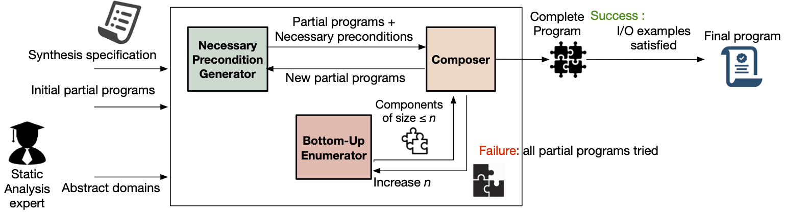
Figure 1. High-level architecture of our synthesis algorithm.

Fig. 1 depicts the overall architecture of our synthesis algorithm, inspired by a recently proposed synthesis strategy (Lee, 2021). The algorithm takes synthesis specification comprising input-output examples, initial partial programs with missing parts as input. Additionally, it requires an abstract domain designed by domain experts that characterizes the abstract semantics of the target language. Our algorithm consists of three key modules, namely Bottom-up enumerator, Necessary precondition generator, and Composer:

• Bottom-up enumerator: Given input-output examples and a number $n$ which is initially $1$, the bottom-up enumerator generates components. The components are expressions (of size $\leq n$) that are to be used to complete the missing parts of partial programs. The bottom-up enumerator exhaustively generates components of the size bound modulo observational equivalence.

• Necessary precondition generator: Given a partial program with missing parts, the necessary precondition generator computes necessary preconditions that must be satisfied by the missing expressions in order for the program to satisfy the specification. To do so, it iteratively performs a forward and a backward abstract interpretations. The resulting necessary precondition maps each missing expression to abstract values, which represent an over-approximation of the possible values that the missing expression is allowed to generate in order for the program to satisfy the specification.

• Composer: Given a partial program annotated with necessary preconditions and components, the composer selects which hole to fill with which component and generates a new partial program. When putting a component in a missing part, the composer checks if the necessary precondition of the missing part is satisfied by the component. If no component satisfies any of the necessary preconditions, the partial program is discarded. If a solution cannot be found until all the combinations of components and missing parts are tried, the current set of components is determined to be insufficient. In this case, the bottom-up enumerator is invoked to add larger components (by increasing $n$), and the process is repeated.

Our algorithm is guaranteed to find a solution if it exists because the Bottom-up enumerator will eventually generate components to complete the synthesis that satisfies the input-output examples.

We have applied our approach to the SyGuS (Alur et al., 2013) specification language. SyGuS is a standard formation that has established various synthesis benchmarks through annual competitions (Past SyGuS Competition, 2020). SyGuS employs a formal grammar to describe the space of possible programs. Such a grammar is expressible in some SMT theory. We devise highly precise abstract domains specialized for the operators in theories of bitvectors and SAT. By targetting the standard formulation, our synthesis algorithm is applicable for a broad class of SyGuS problems with arbitrary grammars in those theories.

We implemented our algorithm in a tool called Simba. We evaluated Simba on a set of 5 benchmarks from the prior work on various applications: 500 benchmarks from program deobfuscation (David et al., 2020), 369 benchmarks from program optimization (Lee et al., 2020), and 1006 benchmarks from the SyGuS competition (synthesizing side-channel resistant circuits and bit-twiddling tricks) (Past SyGuS Competition, 2020). Our evaluation results show that Simba is more scalable than the state-of-the-art tools for inductive SyGuS problems Duet (Lee, 2021) and Probe (Barke et al., 2020). For example, for the 544 non-conditional bitvector-manipulation problems, Simba is able to solve 519 problems in less than 34.8 seconds on average per problem, compared to only 456 and 409 by Duet and Probe using 165.3 and 63.7 seconds on average, respectively. Simba provides significant speedup over the state-of-the-art tools.

We summarize the main contributions of our work:

• A novel and general synthesis algorithm that prunes the search space effectively by using both forward and backward abstract interpretation: Unlike existing synthesis algorithms, our algorithm uses both forward and backward reasoning thus fully exploit the power of abstract interpretation to prune the search space.

• A highly precise abstract domain for bitvectors and SAT: We devise precise forward and backward abstract transfer functions for bitvector and boolean operators. The resulting abstract domains are highly precise and can be used for inductive SyGuS problems with arbitrary grammars in the theories of bitvectors and SAT.

• Implementation and evaluation of our algorithm: We implemented our algorithm in a tool called Simba and evaluated it on a set of 5 benchmarks from a variety of applications. The results show significant performance gains over the existing state-of-the-art synthesis techniques.

1.0.0.1 Limitations.

Our method requires a highly precise abstract domain for the target application. In this paper, we have shown that our algorithm is effective for synthesizing bit-vector and Boolean expressions thanks to our highly precise abstract domains. However, whether our algorithm is effective for other applications (e.g., synthesizing programs with loops, or synthesizing string-manipulating programs) remains an open question. We discuss possible directions for future work in Section 7.

2. Overview

We illustrate our method on the problem of synthesizing a bit-manipulating program. The desired program is a function $f$ that takes as input a bit-vector of fixed-width $4$ denoted $x$ and turns off all bits left to the rightmost 0-bit in $x$. Let us represent bit-vectors as binary numbers. For example, given a bit-vector $1011_{2}$, the function is supposed to return $0011_{2}$.

This problem is represented in SyGuS language, which formulates a synthesis problem as a combination of a syntactic specification and a semantic specification. The syntactic specification for $f$ is the following grammar:

$$\begin{array}[]{rclr}S&\rightarrow&x\;|\;0001_{2}&\text{input bit-vector and bit-vector literals}\\ &\mid&S\land S\;|\;S\lor S\;|\;S\oplus S&\text{bitwise logical binary operators}\\ &\mid&S+S\;|\;S\times S\;|\;S/S\;|\;S>\!>S&\text{bitwise arithmetic binary operators}\end{array}$$

where $S$ is the start non-terminal symbol, and the operators are the ones supported in the theory of bit-vectors ($\oplus$ denotes the bitwise exclusive-or operator and $>\!>$ denotes the arithmetic right shift operator where the leftmost bits are filled with the most significant bit of the left operand). The semantic specification for $f$ follows the programming-by-example (PBE) paradigm and comprises input-output examples. For ease of exposition, we assume only one input-output example is given: $f(1011_{2})=0011_{2}$. A solution to the synthesis problem is $f(x)=((x+0001_{2})\oplus x)>\!>0001_{2}$.

2.0.0.1 Abstract Domain.

In our abstract interpretations we use the following abstract domain of bit-vectors to represent the abstract semantics of the program. The bitwise domain is a set of elements each of which is a sequence of abstract bits of length $4$. Each abstract bit has a value from the set $\{0,1,\bot,\top\}$ where $\top$ represents the unknown value and $\bot$ represents no value. The domain has abstract operators for the bitwise logical and arithmetic operators. The abstract operators simulate the behaviors of the concrete operators in the abstract domain. From now on, we denote each abstract operator in this domain by the corresponding concrete operator with a superscript $\#$. For example, $1\top 10\land^{\#}00\top\top=00\top 0$.

2.0.0.2 Generation of Initial Partial Programs.

We first generate a fixed set $Q$ of partial programs which have one or more non-terminal symbols as placeholders. Starting from the start symbol $S$, we exhaustively generate all possible partial programs by applying the production rules of the grammar to non-terminal symbols up to a certain depth. In this example, for illustration purpose, we assume that the $Q$ set has three partial programs:

$$Q=\{(S\oplus x)>\!>0001_{2},(S/x)>\!>0001_{2},S_{1}\times S_{2}\}$$

2.0.0.3 Component Generation.

The component generator then generates a set $C$ of components by the bottom-up enumerative search, which maintains a set of complete programs and progressively generates new programs by composing existing ones. The set of components consists of expressions of size $\leq n$ where $n$ is the size upperbound which is initially $1$. This upperbound is increased by $1$ whenever the current set of components is insufficient to synthesize a solution. The number of components is potentially exponential to $n$, but we can reduce the number of components by exploiting observational equivalence of expressions. For example, if $x$ is in the component set, $x\lor 0000_{2}$ is not added to the set because they are observationally equivalent. Because initially $n=1$, the component set is

$$C=\{x,0001_{2}\}.$$

These components are used to complete the missing parts (i.e., nonterminals) of the partial programs in $Q$ in the following composition phase.

2.0.0.4 Derivation of Necessary Preconditions.

Before we start the composition phase, we derive a necessary precondition over each subexpression (including nonterminals) of the partial programs in $Q$ using forward and backward analyses using the abstract domain. A necessary precondition is represented as an element in the bitwise abstract domain. The followings are the derivation of necessary preconditions for the partial programs in $Q$.

• $S_{1}\times S_{2}$ (necessary preconditions: $S_{1}\mapsto\top\top\top\top,S_{2}\mapsto\top\top\top\top$): We first perform a forward analysis on the partial program to obtain invariants over the program’s final output and the results of intermediary operations. The nonterminals can be replaced by any expressions, so the abstract output of both nonterminals is $\top\top\top\top$. Thus, the abstract output of the entire program is $\top\top\top\top$. Now we check the feasiblity of the partial program by checking whether the abstract output of the partial program is consistent with the desired output example. This check can be simply done by applying the meet operator ($\sqcap$) to the abstract output of the partial program and the abstraction of the desired output. Because the result does not contain $\bot$ ($\top\top\top\top\sqcap 0011=0011$), the partial program is feasible. Now the backward analysis can be performed to obtain necessary preconditions over the non-terminals. From the desired output $0011_{2}$, considering possible overflows in the multiplication, $S_{1}$ and $S_{2}$ can be any value. Therefore, the necessary precondition of $S_{1}$ (and $S_{2}$) is $\top\top\top\top$.

• $(S\oplus x)>\!>0001_{2}$ (necessary precondition: $S\mapsto 110\top$): By the forward analysis, the abstract output of $(S\oplus x)$ is $\top\top\top\top$, and the abstract output of $(S\oplus x)>\!>0001_{2}$ is $\top\top\top\top>\!>^{\#}0001=\top\top\top\top$. Now we check the feasiblity of the partial program. Becaues the result is not inconsistent with the desired output ($\top\top\top\top\sqcap 0011=0011$), the partial program is feasible. Now the backward analysis is performed. From the desired output $0011_{2}$, we can derive the necessary precondition over $(S\oplus x)$ as $011\top$ because $011\top>\!>^{\#}0001=0011$. The necessary precondition over $S$ is $110\top$ because, for the input $1011_{2}$ for $x$, $110\top\oplus^{\#}1011=011\top$.

• $(S/x)>\!>0001_{2}$ (the program is infeasible): By the forward analysis, the abstract output of $(S/x)$ is $000\top$. That is because from the fact that the maximum possible value of $S$ is $1111_{2}$ (which is $15$ in decimal) and the input $x$’s value is $1011_{2}$ (which is $11$ in decimal), the possible values of $(S/x)$ are $0$ and $1$, which is represented as $000\top$ in the bitwise domain. The abstract output of $(S/x)>\!>0001_{2}$ is $0000$ because $000\top>\!>^{\#}0001=0000$. Now we check the feasiblity of the partial program. Because the result is inconsistent with the desired output ($0000\sqcap 0011=00\bot\bot$), the partial program is infeasible.

As shown in the above, the partial program $(S/x)>\!>0001_{2}$ is determined to be infeasible. Only the other two partial programs will be considered in the composition phase.

2.0.0.5 Composition Process.

Given the partial programs in $Q$ with necessary preconditions and the set $C$ of components, the composer generates new (partial) programs by replacing non-terminal symbols in the partial programs with components.

The composer first chooses $(S\oplus x)>\!>0001_{2}$. It then searches for a component $c$ in $C=\{x,0001_{2}\}$ such that the necessary precondition over $S$ is subsumed by the abstract output of $c$. There is no such component because the necessary precondition $110\top$ is not subsumed by neither of the abstract outputs of $x$ ($1011$) and $0001_{2}$ ($0001$). Therefore, the composer discards the partial program.

The next partial program is $S_{1}\times S_{2}$. Suppose the composer replaces $S_{1}$ with $x$, obtaining a new partial program $x\times S_{2}$. Whenever a new partial program is generated, the necessary precondition generator is invoked to derive necessary preconditions over the non-terminals. Because the multiplication operation is modulo $2^{4}$, computing the necessary precondition over $S_{2}$ amounts to solving the following equation:

$$1011_{2}\times y=0011_{2}\quad{\rm mod}\ 16$$

where $y$ represents the unknown value of $S_{2}$. Using the extended Euclidean algorithm, we can find the solution to the equation as $y=1001_{2}$. Thus, the necessary precondition over $S_{2}$ is $1001$. Unfortunately, there is no component in $C$ whose abstract output subsumes the necessary precondition. Therefore, the composer discards the partial program.

Because the composer exhausts all the partial programs in $Q$ without finding a solution, it invokes the component generator to generate more components.

Next, suppose the component generator generates components of size $\leq 3$ resulting in $C=\{x,0001_{2},x+0001_{2},\cdots\}$.

The composer revisits the partial program $(S_{1}\oplus x)>\!>0001_{2}$. Recall the necessary precondition over $S_{1}$ is $110\top$. Now the component $x+0001_{2}$ whose output is $1100_{2}$ satisfies the necessary precondition. Therefore, the composer replaces $S_{1}$ with $x+0001_{2}$ to obtain a new program $((x+0001_{2})\oplus x)>\!>0001_{2}$. After evaluation of the program, the composer finds that the program is correct and returns it as a solution.

The rest of the paper is organized as follows. Section 3 introduces preliminary concepts and describes our overall synthesis algorithm. Section 4 presents our abstract domains specialized for the theories of bitvectors and Boolean logic. Section 5 presents our experimental results. Section 6 discusses related work. Section 7 discusses future work. Section 8 concludes.

3. Overall Synthesis Algorithm

In this section, we formulate our method. We first introduce preliminary concepts including terms, regular tree grammars, and syntax-guided synthesis over a finite set of examples. We then present our generic synthesis algorithm, which is based on iterative forward-backward abstract interpretation.

3.1. Preliminaries

3.1.0.1 Term

A signature $\Sigma$ is a set of function symbols, where each $f\in\Sigma$ is associated with a non-negative interger $n$, the arity of $f$ (denoted $arity(f)$). For $n\geq 0$, we denote the set of all n-ary elements $\Sigma$ by $\Sigma^{(n)}$. Function symbols of 0-arity are constants. Let $V$ be a set of variables. The set $T_{\Sigma,V}$ of all $\Sigma$-terms over $V$ is inductively defined; $V\subseteq T_{\Sigma,V}$ and $\forall n\geq 0,f\in\Sigma^{(n)}.~{}t_{1},\cdots,t_{n}\in T_{\Sigma,V}.~{}f(t_{1},\cdots,t_{n})\in T_{\Sigma,V}$. A term can be viewed as a tree.

3.1.0.2 Position

The set of positions of term $s$ is a set $\mathit{Pos}(s)$ of strings over the alphabet of natural numbers, which is inductively defined as follows:

• If $s=x\in V$, $\mathit{Pos}(s)=\{\epsilon\}$.

• If $s=f(s_{1},\cdots,s_{n})$, then $\mathit{Pos}(s)=\{\epsilon\}\cup\bigcup^{n}_{i=1}\{ip\mid p\in\mathit{Pos}(s_{i})\}$.

The position $\epsilon$ is called the root position of term $s$. For $p\in\mathit{Pos}(s)$, the subterm of $s$ at position $p$, denoted by $s\mid_{p}$, is defined by (i) $s\mid_{\epsilon}=s$ and (ii) $f(s_{1},\cdots,s_{n})\mid_{iq}=s_{i}\mid_{q}$. For $p\in\mathit{Pos}(s)$, we denote by $s[p\leftarrow t]$ the term that is obtained from $s$ by replacing the subterm at position $p$ by $t$. Formally, $s[\epsilon\leftarrow t]=t$ and $f(s_{1},\cdots,s_{n})[iq\leftarrow t]=f(s_{1},\cdots,s_{i}[q\leftarrow s],\cdots,s_{n})$.

3.1.0.3 Regular Tree Grammar.

A regular tree grammar is a tuple $G=(N,\Sigma,S,\delta)$ where $N$ is a finite set of nonterminal symbols (of arity 0), $\Sigma$ is a signature, $S\in N$ is an initial nonterminal, and $\delta$ is a finite set of productions of the form $A_{0}\to\sigma^{(i)}(A_{1},\cdots,A_{i})$ where each $A_{j}\in N$ is a nonterminal. Given a tree (or a term) $t\in T_{\Sigma,V}$, applying a production $r=A\to\beta$ into $t$ replaces an occurrence of $A$ in $t$ with the right-hand side $\beta$. A tree $t\in T_{\Sigma,V}$ is generated by the grammar $G$ iff it can be obtained by applying a sequence of productions $r_{1},\cdots,r_{n}$ to the tree of which root node represents the initial nonterminal $S$. All the trees that can be derived from $S$ are called the language of $G$ and denoted by $L(G)$.

3.1.0.4 Inductive Syntax-Guided Synthesis

The syntax-guided synthesis problem (Alur et al., 2013) is a tuple $\langle G,\Phi\rangle$. The goal is to find a program $P$ that satisfies a given specification $\Phi$ in a decidable theory. Programs must be written in a language $L(G)$ described by a regular-tree grammar $G$. In particular, we say a SyGuS instance is inductive if the specification is a set of input-output pairs $\Phi=\bigcup^{m}_{j=1}\{i_{j}\mapsto o_{j}\}$ where $i_{j}$ and $o_{j}$ are values . Assuming a deterministic semantics $\left\llbracket{P}\right\rrbracket$ is assigned to each program $P$ in $L(G)$, the goal is to find a program $P$ such that $\left\llbracket{P}\right\rrbracket(i)=o$ for all $i\mapsto o\in\Phi$ (denoted $P\models\Phi$).

3.2. Overall Algorithm

Algorithm 1 The Simba Algorithm

1:A SyGuS instance $\langle G,\Phi=\bigcup^{m}_{j=1}\{i_{j}\mapsto o_{j}\}\rangle$ where each $i_{j},o_{j}\in D$

2:Abstract domain $\hat{D}$ such that $\mathcal{P}\left({D}\right)\mathrel{\begin{subarray}{c}\gamma\\[-1.93748pt] \xleftarrow{\rule{28.45274pt}{0.0pt}}\\[-3.09999pt] \xrightarrow{\rule{28.45274pt}{0.0pt}}\\[-2.71246pt] \alpha\end{subarray}}\hat{D}$

3:An integer $d$ for the maximum height of the partial programs

4:A solution program $P\in L(G)$ that satisfies $\Phi$

5:$Q:=\textsc{GenerateSketches}(G,d)$

6:$n:=1$

7:${\bf C}:=\emptyset$

8:repeat

9:    $Q^{\prime}:=Q$

10:    ${\bf C}:=\textsc{GenerateComponent}(G,{\bf C},n)$ $\triangleright$ ${\bf C}:N\to\mathcal{P}\left({L(G)}\right)$

11:    while $Q^{\prime}$ is not empty do

12:         remove $P$ from $Q^{\prime}$

13:         if IsComplete($P$) and $P\models\Phi$ then return $P$

14:         else

15:             $\mathcal{A}:=\textsc{Analyze}(P,\Phi)$ $\triangleright$ $\mathcal{A}:\mathit{Pos}(P)\to\hat{D}^{m}$

16:             if $\exists p\in\mathit{Pos}(P).~{}\bot_{\hat{D}}\in\mathcal{A}(p)$ then continue

17:             $pos:=\textsc{Pick}(\textsf{Holes}(P))$ $\triangleright$ $pos\in\mathit{Pos}(P)$

18:             for $c\in{\bf C}(P\mid_{pos})$ s.t. $\langle\alpha(\left\llbracket{c}\right\rrbracket(i_{1})),\cdots,\alpha(\left\llbracket{c}\right\rrbracket(i_{m}))\rangle\sqsubseteq\mathcal{A}(pos)$ do

19:                 $Q^{\prime}:=Q^{\prime}\cup\{P[pos\leftarrow c]\}$

20:             end for

21:         end if

22:    end while

23:    $n:=n+1$

24:until false

Now we describe our algorithm of bidirectional search-based inductive synthesis accelerated by using forward/backward abstract interpretation. Algo. 1 shows the high-level structure of our synthesis algorithm, which takes

• Inductive SyGuS instance with a regular tree grammar $G$ and $m$ input-output examples $\Phi$

• Abstract domain $\hat{D}$ that abstracts the set $D$ of values of all terms in $L(G)$ and a Galois connection $\alpha:\mathcal{P}\left({D}\right)\to\hat{D}$ and $\gamma:\hat{D}\to\mathcal{P}\left({D}\right)$

• Integer $d$ that specifies the maximum height of the sketches (partial programs with nonterminals) to be explored

The sketches of height $\leq d$ are enumerated top-down according to the grammar $G$, and inserted into the priority queue $Q$ (line 5). Then, the size upperbound $n$ for components is initially set to be $1$ (line 6). The integer $n$ will be increased by $1$ at each iteration (line 23) until a solution is found. The component pool ${\bf C}$ (which is initially the empty set) includes all the components of size $\leq n$ that are generated in a bottom-up fashion. The main loop (lines 8–24) is repeated until a solution is found. The priority queue $Q^{\prime}$ which will be used in a current iteration is initialized by inserting the sketches in $Q$ into $Q^{\prime}$ (line 9). The GenerateComponent procedure incrementally builds expressions of size $\leq n$ by composing the previously generated expressions (line 10). By exploiting the observational equivalence, ${\bf C}$ does not include multiple components which are semantically equivalent to each other with respect to the specification. In the while loop (lines 11–22), the algorithm explores the search space determined by the current component pool ${\bf C}$ and the set of sketches. If a candidate $P$ dequeued from $Q^{\prime}$ is a complete program and correct with respect to the specification, $P$ is returned as a solution (line 13). Otherwise, another candidate in $Q^{\prime}$ is explored. If a candidate $P$ is a partial program, we analyze $P$ to infer a necessary precondition for each subexpression in $P$. The Analyze procedure computes a map $\mathcal{A}$ that maps each subexpression in $P$ to a tuple of $m$ abstract values in $\hat{D}$ (line 15). The $j$-th abstract value represents a necessary precondition to be satisfied any expression that is substituted for the nonterminal in order to satisfy the $j$-th input-output example $i_{j}\mapsto o_{j}$. If $P$ has a position having $\bot_{\hat{D}}$ representing no expression can be put in that position, $P$ is determined to be infeasible and discarded (line 16). Otherwise, a nonterminal in $P$ is chosen (line 17). For each component $c$ that can be substituted for the nonterminal and satisfies the necessary precondition (line 18), we replace the nonterminal with $c$ and enqueue the resulting program into $Q^{\prime}$ (line 19). If no solution is found with the current component pool ${\bf C}$, the size $n$ is increased by $1$ (line 23) and the main loop is repeated.

Our algorithm has the following properties. First, our algorithm is sound and complete in the following sense.

Theorem 3.1.

Algo. 1 is sound and complete in the sense that if a solution to a given inductive SyGuS instance exists, Algo. 1 eventually finds the solution.

Second, it can determine the unrealizability (Hu et al., 2020) of a given inductive SyGuS instance if every sketch in the queue $Q^{\prime}$ has a position having $\bot_{\hat{D}}$ and discarded at line 16 in the main loop. That is, no sketch can be completed to a feasible program. Lastly, it can be solely used for top-down synthesis rather than bidirectional synthesis, which makes it applicable to existing top-down synthesis algorithms. To do so, instead of using a fixed set of sketches, at each iteration of the main loop (lines 8–24), we can add larger sketches to the queue $Q^{\prime}$ by increasing the maximum height $d$ of the sketches to be explored while keeping the size upperbound $n$ to be $1$ until a solution is found.

3.3. The Iterative Forward-Backward Analysis

We describe the Analyze procedure in Algo. 1 in detail. It is known that by alternating forward and backward analyses, we can compute an overapproximation of the set of states that are both reachable from the program entry and able to reach a desired state at the program exit (Cousot and Cousot, 1992). In our setting where a program is a tree, execution of a program starts at the leaves of the program tree (constants or the input variable) and proceeds to the root. Therefore, for each node of the program tree, a forward analysis computes an over-approximation of the set of values that may be computed from a subtree rooted at the node in a bottom-up manner. A backward analysis computes an over-approximation of the set of values that may be used to generate output desired by its parent in a top-down fashion.

Given a candidate $P$ and $n$ input-output examples $\Phi$, the Analyze procedure performs the iterative forward-backward analysis for each input-output example and combines the results to obtain a map $\mathcal{A}$. The analysis result $\mathcal{A}$ maps each position in $P$ to a tuple of abstract values $\hat{d}_{1},\cdots,\hat{d}_{m}$.

The forward abstract semantics with respect to an input-output example $i\mapsto o$ is characterized by the least fixpoint of the following function $\mathcal{F}_{\langle i,o\rangle}:(\mathit{Pos}(P)\to\hat{D})\to(\mathit{Pos}(P)\to\hat{D})$:

$$\begin{array}[]{cc}\mathcal{F}_{\langle i,o\rangle}=\lambda X.~{}\mathcal{I}^{i}_{\mathcal{F}}\sqcup F^{\#}(X)&\text{where}\quad\mathcal{I}^{i}_{\mathcal{F}}=\{p\mapsto\left\{\begin{array}[]{ll}\alpha(i)&(P\mid_{p}\in V)\\ \top&(P\mid_{p}\in N)\\ \alpha(P\mid_{p})&(P\mid_{p}\text{ is a constant})\\ \bot&(\text{otherwise})\end{array}\right.\mid p\in\mathit{Pos}(P)\}.\end{array}$$

The initial state $\mathcal{I}^{i}_{\mathcal{F}}$ maps each nonterminal in $N$ to $\top$ since a nonterminal represents a hole that can be filled by any expression. Each variable is mapped to the abstraction of the input example (i.e., $\alpha(i)$), and each constant is mapped to the abstraction of the constant itself. The forward abstract function $F^{\#}$ is defined as follows:

$$\small F^{\#}(X)=\{p\mapsto\left\{\begin{array}[]{ll}\overrightarrow{f}^{\#}(X(p1),\cdots,X(pk))&(P\mid_{p}=f(\cdots),arity(f)=k)\\ \bot&(\text{otherwise})\end{array}\right.\mid p\in\mathit{Pos}(P)\}$$

where $\overrightarrow{f}^{\#}$ denotes the forward abstract operator of an operator $f$. It takes abstract values of arguments and returns a resulting abstract value.

The backward abstract semantics with respect to an input-output example $i\mapsto o$ is characterized by the greatest fixpoint of the following function $\mathcal{B}_{\langle i,o\rangle}:(\mathit{Pos}(P)\to\hat{D})\to(\mathit{Pos}(P)\to\hat{D})$:

$$\begin{array}[]{cc}\mathcal{B}_{\langle i,o\rangle}=\lambda X.~{}\mathcal{I}^{o}_{\mathcal{B}}\sqcap B^{\#}(X)&\text{where}\quad\mathcal{I}^{o}_{\mathcal{B}}=\{p\mapsto\left\{\begin{array}[]{ll}\alpha(o)&(p=\epsilon)\\ \top&(\text{otherwise})\end{array}\right.\mid p\in\mathit{Pos}(P)\}.\end{array}$$

The final state $\mathcal{I}^{o}_{\mathcal{B}}$ maps the root position to the abstraction of the output example (i.e., $\alpha(o)$) and every other position to $\top$. The backward abstract function $B^{\#}$ is defined as follows:

$$\small B^{\#}(X)=\{p\mapsto\left\{\begin{array}[]{ll}\overleftarrow{f}^{\#}_{i}(X(p^{\prime}),X(p^{\prime}1),\cdots,X(p^{\prime}k))&(p=p^{\prime}i,P\mid_{p^{\prime}}=f(\cdots),arity(f)=k)\\ \top&(\text{otherwise})\end{array}\right.\mid p\in\mathit{Pos}(P)\}$$

where $\overleftarrow{f}^{\#}_{i}$ denotes the backward abstract operator of an operator $f$. It takes an abstract value of the result and abstract values of arguments, and returns an abstract value of the $i$-th argument, which corresponds to the necessary precondition for the $i$-th argument to satisfy the input-output example.

The intersection of the forward and backward abstract semantics is computed by obtaining the limit of the following decreasing chain defined for all $n\in\mathbb{N}$ until the chain converges (Cousot and Cousot, 1992): $\dot{X}^{0}_{\langle i,o\rangle}=\texttt{{\it lfp\/}}\ \mathcal{F}_{\langle i,o\rangle}$, $\dot{X}^{2n+1}_{\langle i,o\rangle}=\texttt{{\it gfp\/}}\ \lambda X.~{}\dot{X}^{2n}_{\langle i,o\rangle}\sqcap\mathcal{B}_{\langle i,o\rangle}(X)$, and $\dot{X}^{2n+2}_{\langle i,o\rangle}=\texttt{{\it lfp\/}}\ \lambda X.~{}\dot{X}^{2n+1}_{\langle i,o\rangle}\sqcap\mathcal{F}_{\langle i,o\rangle}(X)$.

The Analyze procedure is defined as follows:

$$\small\textsc{Analyze}(P,\bigcup^{m}_{j=1}i_{j}\mapsto o_{j})\!=\!\{p\mapsto\langle\mathcal{A}_{1}(p),\cdots,\mathcal{A}_{m}(p)\rangle\mid p\in\mathit{Pos}(P),\forall 1\leq j\leq m.~{}\mathcal{A}_{j}\!=\!\lim_{n\to\infty}\dot{X}^{n}_{\langle i_{j},o_{j}\rangle}\}$$

Example 3.2.

Consider the partial program $P=(S\oplus x)>\!>0001_{2}$ in the overview example in Section 2 where the input example $i=1011_{2}$ and the output example $o=0011_{2}$. The subterms of $P$ are $(S\oplus x)$, $0001_{2}$, $S$, and $x$, and their positions are $1$, $2$, $11$, and $12$, respectively. Assuming that the abstract domain $\hat{D}$ is the bitwise domain, the initial state for the forward analysis $\mathcal{I}^{i}_{\mathcal{F}}$ is $\{\epsilon\mapsto\bot\bot\bot\bot,1\mapsto\bot\bot\bot\bot,2\mapsto 0001,11\mapsto\top\top\top\top,12\mapsto 1011\}$. The initial state for the backward analysis $\mathcal{I}^{o}_{\mathcal{B}}$ maps the root position $\epsilon$ to $0011$ and every other position to $\top\top\top\top$. The table below shows the first three elements of the decreasing chain $\dot{X}^{n}_{\langle i,o\rangle}$:

Position $p$	$\dot{X}^{0}_{\langle i,o\rangle}(p)$	$\dot{X}^{1}_{\langle i,o\rangle}(p)$	$\dot{X}^{2}_{\langle i,o\rangle}(p)$
$\epsilon$	$\top\top\top\top$	$0011$	$0011$
$1$	$\top\top\top\top$	$011\top$	$011\top$
$2$	$0001$	$0001$	$0001$
$11$	$\top\top\top\top$	$110\top$	$110\top$
$12$	$1011$	$1011$	$1011$

We assume the forward and backward abstract operators in the bitwise domain defined for the bitwise XOR operator and the arithmetic right shift operator (described in Section 4) are used. Because the chain converges at $\dot{X}^{2}_{\langle i,o\rangle}$, the Analyze procedure returns it as the final result.

3.4. Optimizations

In the implementation, we apply the following optimizations to improve the efficiency of Algo. 1.

3.4.0.1 Concretization to Avoid Unnecessary Scans.

In addition to the component pool ${\bf C}:N\to\mathcal{P}\left({L(G)}\right)$ that memorizes the component expressions derivable from each nonterminal, we also maintain an additional map ${\bf V}:N\to(D\times D)\to\mathcal{P}\left({L(G)}\right)$ that returns components that exhibit a certain input-output behavior. For example, in the overview example in Section 2, ${\bf V}(S)(1011_{2},1100_{2})=\{x+0001_{2}\}$ because $x+0001_{2}$ outputs $1100_{2}$ when given $1011_{2}$ as input. This map is used to save the time for line 18 only when the analysis result $\mathcal{A}(pos)$ is precise enough (i.e., its concretization result is a small set). In such a case, instead of computing the set $\{c\in{\bf C}(P\mid_{pos}\mid\langle\alpha(\left\llbracket{c}\right\rrbracket(i_{1})),\cdots,\alpha(\left\llbracket{c}\right\rrbracket(i_{m}))\rangle\sqsubseteq\mathcal{A}(pos))\}$, we compute $\bigcap\{{\bf V}(P\mid_{pos})(i_{j},v_{j})\mid\mathcal{A}(pos)=\langle\hat{d}_{1},\cdots,\hat{d}_{m}\rangle,\forall 1\leq j\leq m.~{}v_{j}\in\gamma(d_{j})\}$ to obtain the set of components that are compatible with the analysis result. This can save the time for line 18 by avoiding scanning the entire component pool ${\bf C}$.

3.4.0.2 Divide-and-Conquer for Conditional Programs.

In the case of synthesis of conditional programs, we incorporate the divide-and-conquer enumerative approach (Alur et al., 2017) into our algorithm as follows. First, for each input-output example, by using Algo. 1, we synthesize a conditional-free program which satisfies that example. Second, we combine these conditional-free programs into a single conditional program that works for all examples by using the previous decision tree learning algorithm from (Alur et al., 2017). Conditional predicates are generated by bottom-up enumeration.

4. Abstract Domains

In this section, we propose efficient but precise abstract domains that can be used for a wide range of inductivey SyGuS problems with background theories of (1) fixed-width bitvectors and (2) propositional logic.

For a space reason, we only present some noteworthy points of our abstract domains. The full details of our abstract domains are available in the supplementary material.

4.1. Notations

For the theory of bitvectors of fixed-width $w$, we follow the standard syntax and semantics of the bit-vector operators described in the SMT-LIB v2.0 standard (Barrett et al., 2010). Unsigned and signed bit-vectors are represented as bitstrings of length $w$ (i.e., $\{0,1\}^{w}$). The values of unsigned bit-vectors range over $\{0,\cdots,2^{w}-1\}$, and those of signed ones range over $\{-2^{w-1},\cdots,2^{w-1}-1\}$ respectively. We refer to $-2^{w-1}$, $2^{w-1}-1$, $0$, and $2^{w}-1$ as ${\tt smin}$, ${\tt smax}$, ${\tt umin}$, and ${\tt umax}$ respectively. We denote $[n]_{i}$ as $i$-th bit of the bitstring representation of $n$ and $[n]_{i:j}$ as a substring of $n$ comprising $i$-th bit, $i$+1-th bit, $\cdots$, $j$-th bit of $n$. The concatenation of two strings $n_{1}$ and $n_{2}$ is denoted by $n_{1}\cdot n_{2}$, and the length of a string $n$ is denoted by $|n|$. We denote $n[a/b]$ as the bitstring obtained by replacing every occurrence of $b$ in $n$ with $a$. For an interval $[l,h]$, we denote $lb([l,h])$ and $ub([l,h])$ as the lower and upper bounds of $[l,h]$ respectively. Lastly, for a bitstring $n$, we denote $\textsf{Trail0s}(n)$ as the number of trailing zeros in $n$.

4.2. Abstract Domain for Fixed-Width Bitvectors

4.2.0.1 Abstract Domain.

Our abstract domain for fixed-width bitvectors is a reduced product domain. Reduced product of abstract domains can be used to achieve precise abstractions by synergistically combining the expressiveness power of several abstract domains (Cousot, 2021). Our abstract domain comprises the following domains.

The bitwise domain $\langle\hat{B},\sqsubseteq_{\hat{B}},\sqcup_{\hat{B}},\sqcap_{\hat{B}}\rangle$ is a domain that tracks the value of each bit of a bit-vector independently, also used in prior work (Miné, 2012; Regehr and Duongsaa, 2006). Each element of the bitwise domain $\hat{B}$ is a string of abstract bits of length $w$ as already introduced in Section 2. The domain is formally defined as follows: $\hat{B}\stackrel{{\scriptstyle\mathtt{def}}}{{=}}\{b_{1}\cdot b_{2}\cdots b_{w}\mid\forall 1\leq i\leq w.~{}b_{i}\in\{0,1,\bot,\top\}\}$. To define the galois connection between $\hat{B}$ and $\mathcal{P}\left({\mathbb{Z}}\right)$, we define the following function that computes the bit-vector representation $p(x)$ of an integer $x$ using the two’s complement representation (Miné, 2012):

$$\small p(x)\stackrel{{\scriptstyle\mathtt{def}}}{{=}}\left\{\begin{array}[]{ll}b_{1}\cdots b_{w}\quad\text{ where }\forall 1\leq i\leq w.~{}b_{i}=\lfloor x/2^{w-i}\rfloor\mod 2&(x\geq 0)\\ b^{\prime}_{1}\cdots b^{\prime}_{w}\quad\text{ where }\forall 1\leq i\leq w.~{}b^{\prime}_{i}=\neg b_{i},b_{i}=[p(-x-1)]_{i}&(x<0)\\ \end{array}\right.$$

Note that the leftmost bit is the most significant bit. The galois connection $\mathcal{P}\left({\mathbb{Z}}\right)\mathrel{\begin{subarray}{c}\gamma_{\hat{B}}\\[-2.15277pt] \xleftarrow{\rule{28.45274pt}{0.0pt}}\\[-3.44444pt] \xrightarrow{\rule{28.45274pt}{0.0pt}}\\[-3.01385pt] \alpha_{\hat{B}}\end{subarray}}\hat{B}$ is defined as follows:

$$\small\begin{array}[]{ccc}\alpha_{\hat{B}}(Z)\stackrel{{\scriptstyle\mathtt{def}}}{{=}}\bigsqcup_{\hat{B}}\{p(x)\mid x\in Z\}&&\gamma_{\hat{B}}(b)\stackrel{{\scriptstyle\mathtt{def}}}{{=}}\left\{\begin{array}[]{ll}\emptyset&(\exists i.~{}[b]_{i}=\bot)\\ \gamma^{\rm unsigned}_{\hat{B}}(b)\cup\gamma^{\rm signed}_{\hat{B}}(b)&(\text{otherwise})\end{array}\right.\end{array}$$

where the concretization functions for unsigned and signed bit-vectors are defined as follows:

$$\small\begin{array}[]{c}\gamma^{\rm unsigned}_{\hat{B}}(b)\stackrel{{\scriptstyle\mathtt{def}}}{{=}}\{\sum^{w-1}_{i=0}2^{i}m_{w-i}\mid\forall 1\leq i\leq w.~{}m_{i}\in\gamma_{B}([b]_{i})\}\\ \gamma^{\rm signed}_{\hat{B}}(b)\stackrel{{\scriptstyle\mathtt{def}}}{{=}}\{-2^{w-1}m_{1}+\sum^{w-2}_{i=0}2^{i}m_{w-i}\mid\forall 1\leq i\leq w.~{}m_{i}\in\gamma_{B}([b]_{i})\}.\end{array}$$

The signed interval domain $\langle\hat{S},\sqsubseteq_{\hat{S}},\sqcup_{\hat{S}},\sqcap_{\hat{S}}\rangle$ is a domain for representing bitvectors as intervals of signed bit-vectors. Formally, $\hat{S}\stackrel{{\scriptstyle\mathtt{def}}}{{=}}\{[l,h]\mid l,h\in\{0,1\}^{w},\left\llbracket{{\tt bvsle}}\right\rrbracket(l,h)={\tt true}\}$ where ${\tt bvsle}$ is the binary predicate for signed less than or equal. The galois connection $\mathcal{P}\left({\mathbb{Z}}\right)\mathrel{\begin{subarray}{c}\gamma_{\hat{S}}\\[-2.15277pt] \xleftarrow{\rule{28.45274pt}{0.0pt}}\\[-3.44444pt] \xrightarrow{\rule{28.45274pt}{0.0pt}}\\[-3.01385pt] \alpha_{\hat{S}}\end{subarray}}\hat{S}$ is standard.

The unsigned interval domain $\langle\hat{U},\sqsubseteq_{\hat{U}},\sqcup_{\hat{U}},\sqcap_{\hat{U}}\rangle$ is a domain for representing bitvectors as intervals of unsigned bit-vectors. Formally, $\hat{U}\stackrel{{\scriptstyle\mathtt{def}}}{{=}}\{[l,h]\mid l,h\in\{0,1\}^{w},\left\llbracket{{\tt bvule}}\right\rrbracket(l,h)={\tt true}\}$ where ${\tt bvule}$ is the binary predicate for unsigned less than or equal. The galois connection $\mathcal{P}\left({\mathbb{Z}}\right)\mathrel{\begin{subarray}{c}\gamma_{\hat{U}}\\[-2.15277pt] \xleftarrow{\rule{28.45274pt}{0.0pt}}\\[-3.44444pt] \xrightarrow{\rule{28.45274pt}{0.0pt}}\\[-3.01385pt] \alpha_{\hat{U}}\end{subarray}}\hat{U}$ is also standard.

The above three domains are combined to form the product abstract domain $\hat{D}=\hat{B}\times\hat{S}\times\hat{U}$. with the galois connection $\mathcal{P}\left({\mathbb{Z}}\right)\mathrel{\begin{subarray}{c}\gamma\\[-2.15277pt] \xleftarrow{\rule{28.45274pt}{0.0pt}}\\[-3.44444pt] \xrightarrow{\rule{28.45274pt}{0.0pt}}\\[-3.01385pt] \alpha\end{subarray}}\hat{D}$ that can be simply defined by combining the galois connections of the three domains.

To let the information flow among the three domains to mutually refine them, we need to use a reduction operator that exploits the information tracked by one of the three domains to refine the information tracked by the others. The reduction requires to compute a fixpoint (Granger, 1992), and our iterated reduction operator $\rho:\hat{D}\to\hat{D}$ is defined as follows:

$$\small\rho\stackrel{{\scriptstyle\mathtt{def}}}{{=}}\texttt{{\it fix\/}}\ \lambda\langle b,s,u\rangle.~{}\langle b\sqcap\pi_{\hat{S}\to\hat{B}}(s)\sqcap\pi_{\hat{U}\to\hat{B}}(u),s\sqcap\pi_{\hat{B}\to\hat{S}}(b)\sqcap\pi_{\hat{U}\to\hat{S}}(u),u\sqcap\pi_{\hat{B}\to\hat{U}}(b)\sqcap\pi_{\hat{S}\to\hat{U}}(s)\rangle$$

where $\pi_{\hat{D}_{1}\to\hat{D}_{2}}$ is our projection operator that propagates information from abstract domain $\hat{D}_{1}$ to another domain $\hat{D}_{2}$. For example, the $\pi_{\hat{B}\to\hat{U}}$ operator takes a bitwise element and returns an unsigned interval whose lower bound (resp. upper bound) is a bit-vector obtained by replacing every $\top$ abstract bit with 0 (resp. 1). More details can be found at the supplementary material.

A reduction operator $\rho$ in abstract domain $\hat{D}$ should be sound in the sense that it has to satisfy the following two properties: for all $d\in\hat{D}$, (1) $\rho(d)\sqsubseteq d$ (the result of its application is a more precise abstract element); (2) $\gamma(\rho(d))=\gamma(d)$ (an abstract element and its reduction has the same meaning).

Theorem 4.1.

Our reduction operator $\rho$ is sound.

4.2.0.2 Abstract Operators.

Now we define forward and backward abstract operators. Because we deal with binary numbers with a fixed number of digits, all the domains consider possible overflows/underflows. For each bit-vector operation $f$ of arity $k$, the forward abstract operator $\overrightarrow{f}^{\#}:\hat{D}^{k}\to\hat{D}$, which takes $k$ abstract elements of arguments and returns an abstract element of the result, is defined to be

$$\small\overrightarrow{f}^{\#}(\langle b_{1},s_{1},u_{1}\rangle,\cdots,\langle b_{k},s_{k},u_{k}\rangle)=\rho(\langle\overrightarrow{f}^{\#}_{\hat{B}}(b_{1},\cdots,b_{k}),\overrightarrow{f}^{\#}_{\hat{S}}(s_{1},\cdots,s_{k}),\overrightarrow{f}^{\#}_{\hat{U}}(u_{1},\cdots,u_{k})\rangle)$$

where $\overrightarrow{f}^{\#}_{\hat{B}}$, $\overrightarrow{f}^{\#}_{\hat{S}}$, and $\overrightarrow{f}^{\#}_{\hat{U}}$ are the forward operators in the bitwise domain, the signed domain, and the unsigned domain, respectively. For each $1\leq i\leq k$, the backward abstract operator $\overleftarrow{f}^{\#}_{i}:\hat{D}^{k+1}\to\hat{D}^{k}$ takes the current abstract element of the result and $k$ abstract elements of arguments, and returns a more refined abstract element of the $i$-th argument.

$$\small\overleftarrow{f}^{\#}_{i}(\langle b,s,u\rangle,\langle b_{1},s_{1},u_{1}\rangle\cdots\langle b_{k},s_{k},u_{k}\rangle)=\rho(\langle\overleftarrow{f}^{\#}_{\hat{B},i}(b,b_{1}\cdots b_{k}),\overleftarrow{f}^{\#}_{\hat{S},i}(s,s_{1}\cdots s_{k}),\overleftarrow{f}^{\#}_{\hat{U},i}(u,u_{1}\cdots u_{k})\rangle)$$

where $\overleftarrow{f}^{\#}_{\hat{B},i}$, $\overleftarrow{f}^{\#}_{\hat{S},i}$, and $\overleftarrow{f}^{\#}_{\hat{U},i}$ are the backward operators in the bitwise domain, the signed domain, and the unsigned domain, respectively. We always apply the reduction operator whenever we apply the forward or backward operators in order to maintain analysis results in the most precise form.

In the following, we describe the forward and backward operators for each domain. We will use the same bit-vector operator names as the ones defined in the SMT-LIB v2.0 standard.

4.2.0.3 Forward Abstract Operators for the Signed/Unsigned Interval Domains

In the following, we explain some salient features of the forward abstract operators in detail.

• $\overrightarrow{{\tt bvadd}}^{\#}_{\hat{S}}$ is defined similarly to the standard integer interval arithmetic with a slight difference that it is aware of possible overflows/underflows. Formally,

  $$\small\begin{array}[]{rcl}\overrightarrow{{\tt bvadd}}^{\#}_{{\hat{S}}}([l_{1},h_{1}],[l_{2},h_{2}])&=&\textsf{Wrap}_{{\hat{S}}}([\left\llbracket{{\tt bvadd}}\right\rrbracket(l_{1},l_{2}),\left\llbracket{{\tt bvadd}}\right\rrbracket(h_{1},h_{2})])\quad(\overrightarrow{{\tt bvadd}}^{\#}_{{\hat{U}}}\text{ is similar.})\end{array}$$

  where $\textsf{Wrap}_{\hat{S}}([l,h])=[l,h]$ if ($[l,h]\sqsubseteq_{\hat{S}}[{\tt smin},{\tt smax}]$) and $[{\tt smin},{\tt smax}]$ otherwise. The other abstract operators for subtraction, multiplication, and division are similarly defined.

• $\overrightarrow{{\tt bvneg}}^{\#}_{\hat{U}}$ switches the lower and upper bounds of the interval with the exception of the case where the lower bound represents zero and the upper bound represents a non-zero value. That is because the negation of $1$ is $-1$ which is represented as $11\cdots 1_{2}$ in two’s complement representation. $11\cdots 1_{2}$ is the largest value in the unsigned interval domain. Therefore, the top element is returned in this case. Formally,

  $$\small\begin{array}[]{rcl}\overrightarrow{{\tt bvneg}}^{\#}_{\hat{U}}([l,h])&=&\left\{\begin{array}[]{ll}\top_{\hat{U}}&(l=p(0),h\neq p(0))\\[3.87498pt] [\left\llbracket{{\tt bvneg}}\right\rrbracket(h),\left\llbracket{{\tt bvneg}}\right\rrbracket(l)]&(\text{otherwise})\end{array}\right.\\[3.87498pt] \end{array}$$

• $\overrightarrow{{\tt bvsdiv}}^{\#}_{\hat{S}}$ simulates the following concrete semantics of the signed division.

  $$\small\left\llbracket{{\tt bvsdiv}}\right\rrbracket(s,t)=\left\{\begin{array}[]{ll}\left\llbracket{{\tt bvudiv}}\right\rrbracket(s,t)&(\text{if $s$ and $t$ are both non-negative})\\ \left\llbracket{{\tt bvudiv}}\right\rrbracket(\left\llbracket{{\tt bvneg}}\right\rrbracket(s),\left\llbracket{{\tt bvneg}}\right\rrbracket(t))&(\text{if both are negative})\\ \left\llbracket{{\tt bvneg}}\right\rrbracket(\left\llbracket{{\tt bvudiv}}\right\rrbracket(\left\llbracket{{\tt bvneg}}\right\rrbracket(s),t))&(\text{if $s$ is negative and $t$ is non-negative})\\ \left\llbracket{{\tt bvneg}}\right\rrbracket(\left\llbracket{{\tt bvudiv}}\right\rrbracket(s,\left\llbracket{{\tt bvneg}}\right\rrbracket(t)))&(\text{if $s$ is non-negative and $t$ is negative})\end{array}\right.$$

  Following the above semantics, $\overrightarrow{{\tt bvsdiv}}^{\#}_{\hat{S}}$ splits the intervals of the arguments into the four cases and computes the quotient of each case separately using the $\overrightarrow{{\tt bvudiv}}^{\#}$ operator, which is standardly defined.

4.2.0.4 Forward Abstract Operators for the Bitwise Domain

Some remarkable points are as follows:

• $\overrightarrow{{\tt bvadd}}^{\#}_{\hat{B}}$ is defined by the RippleCarryAdd operator defined in (Regehr and Duongsaa, 2006), which simulates the ripple-carry addition of two bit-vectors in the bitwise domain.

• $\overrightarrow{{\tt bvneg}}^{\#}_{\hat{B}}$ is defined from that $\left\llbracket{{\tt bvneg}}\right\rrbracket(b)=\left\llbracket{{\tt bvadd}}\right\rrbracket(\left\llbracket{{\tt bvnot}}\right\rrbracket(b),p(1))$ (Warren, 2012).

• $\overrightarrow{{\tt bvmul}}^{\#}_{\hat{B}}$ is defined from that the number of trailing zeros in the result of $\left\llbracket{{\tt bvmul}}\right\rrbracket(b_{1},b_{2})$ is the sum of the number of trailing zeros in $b_{1}$ and $b_{2}$. Formally,

  $$\begin{array}[]{rcl}\overrightarrow{{\tt bvmul}}^{\#}_{\hat{B}}(b_{1},b_{2})&=&\top^{w-(n+m)}\cdot 0^{(n+m)}\quad\text{ where }n=\textsf{Trail0s}(b_{1}),m=\textsf{Trail0s}(b_{2})\\[4.30554pt] \end{array}$$

• The abstract operators for the arithmetic shift $\overrightarrow{{\tt bvashr}}^{\#}_{\hat{B}}$ is defined using the shift-right operators in the bitwise domain defined as follows: $b>\!>^{\#}_{x}i$ shifts all the abstract bits of $b$ to the right by $i$ bits, and the leftmost bits are filled with $x$. Formally,

  $$\small\begin{array}[]{rcl}\overrightarrow{{\tt bvashr}}^{\#}_{\hat{B}}(b_{1},b_{2})&=&\bigsqcup\{b_{1}>\!>^{\#}_{[b_{1}]_{1}}(i\mod w)\mid i\in\gamma^{\rm unsigned}_{\hat{B}}(b_{2})\}.\end{array}$$

  The other abstract shift operators are similarly defined.

4.2.0.5 Backward Abstract Operators for the Signed/Unsigned Interval Domains

Some noteworthy points are as follows:

• $\overleftarrow{{\tt bvurem}}^{\#}_{\hat{U},1}(i,i_{1},i_{2})$ refines the abstract value of the first operand ($i_{1}$) from abstract values of the second operand ($i_{2}$) and the result ($i$), and is defined as follows:

  $$\small\begin{array}[]{rcl}\overleftarrow{{\tt bvurem}}^{\#}_{\hat{U},1}(i,i_{1},i_{2})&=&\left\{\begin{array}[]{ll}i\sqcap_{\hat{U}}i_{1}&(\left\llbracket{{\tt bvule}}\right\rrbracket(p(2^{w-1}),lb(i))={\tt true})\\ \top&(\text{otherwise})\end{array}\right.\end{array}$$

  This behavior is based on the fact that for some bit-vectors $b_{1}$, $b_{2}$, and $b$, if $\left\llbracket{{\tt bvurem}}\right\rrbracket(b_{1},b_{2})=b$ and the most significant bit of $b$ is 1, then $b=b_{1}$. The proof is available in the supplementary material.

4.2.0.6 Backward Abstract Operators for the Bitwise Domain

Some noteworthy operators are as follows:

• $\overleftarrow{{\tt bvand}}^{\#}_{\hat{B},1}$ infers the abstract value of the left operand of ${\tt bvand}$ from the abstract values of the other operand and the result. For example, for each abstract bit of the result, if the bit is $1$, we can infer that the corresponding bit of the first operand is $1$ as well. Formally,

  $$\small\begin{array}[]{rcl}\overleftarrow{{\tt bvand}}^{\#}_{\hat{B},1}(b,b_{1},b_{2})&=&d_{1}d_{2}\cdots d_{w}\quad\text{ where }\forall 1\leq i\leq w.~{}d_{i}=\left\{\begin{array}[]{ll}1&([b]_{i}=1)\\ 0&([b]_{i}=0,[b_{2}]_{i}=1)\\ \top&(\text{otherwise})\end{array}\right.\end{array}$$

  The abstract operators for the other bitwise logical operators are defined similarly.

• For $\overleftarrow{{\tt bvshl}}^{\#}_{\hat{B},1}(b,b_{1},b_{2})$, if the shift amount is a constant, we can infer the abstract value of the first operand by shifting $b$ to the right (i.e., reverse direction) by the shift amount. However, the shift amount is not exactly known in general, so we should overapproximate it. We apply the join operator into the results of shifting $b$ to the right by all possible shift amounts. The minimum shift amount is zero and the maximum shift amount is the number of trailing zeros of $b$ obtainable assuming every unknown bit ($\top$) is $0$. This range can be more refined by considering the abstract value of the second operand. Formally,

  $$\small\begin{array}[]{rcl}\overleftarrow{{\tt bvshl}}^{\#}_{\hat{B},1}(b,b_{1},b_{2})&=&\bigsqcup\{b>\!>^{\#}_{\top}(n\ {\rm mod}\ w)\mid n\in\gamma_{\hat{U}}([0,\textsf{Trail0s}(b[0/\top])]\sqcap\pi_{\hat{B}\to\hat{U}}(b_{2}))\}\end{array}$$

• $\overleftarrow{{\tt bvmul}}^{\#}_{\hat{B},1}$ is most complicated among the backward abstract operators, which is defined as follows:

  $$\small\begin{array}[]{l}\overleftarrow{{\tt bvmul}}^{\#}_{\hat{B},1}(b,b_{1},b_{2})=\left\{\begin{array}[]{ll}\textsf{InferMulOp}(b_{2},b)&(|\gamma^{\rm unsigned}_{\hat{B}}(b_{2})|=|\gamma^{\rm unsigned}_{\hat{B}}(b)|=1)\\ \top^{w-l}\cdot 0^{l}&(\text{otherwise})\\ \end{array}\right.\\[3.87498pt] \qquad\text{where }l=\max\{0,\textsf{Trail0s}(b)-\textsf{Trail0s}(b_{2}[0/\top])\}\end{array}$$

  where the InferMulOp will be defined soon. This backward abstract operator precisely infers the abstract value of the first operand if the second operand and the result are exactly known. Suppose the second operand and the result represent non-negative numbers $n_{2}$ and $n$ respectively . Because the multiplication is modulo $2^{w}$, our goal is to find $x$ such that

  (1) $$x\times n_{2}\equiv n\quad(\textrm{mod}\ 2^{w})$$

  When both $n_{2}$ and $n$ are not zero, we can find $x$ as follows (cases where $n_{2}$ or $n$ is zero are trivial): let the numbers of trailing zeros of $b_{2}$ and $b$ are $t_{2}$ and $t$ respectively. Because $n_{2}\neq 0\land n\neq 0$, $n_{2}=2^{t_{2}}\times m_{2}$ and $n=2^{t}\times m$ for some odd numbers $m_{2}$ and $m$. We have two cases.

  • Case 1) $t\geq t_{2}$: We can transform the equation (1) into $x\times(n_{2}/2^{t_{2}})\equiv(n/2^{t_{2}})\quad(\textrm{mod}\ 2^{w-t_{2}})$ because $n_{2}/2^{t_{2}}$ is odd, $n_{2}/2^{t_{2}}$ and $2^{w-t_{2}}$ are coprime. By the extended Euclidean algorithm, we can find the modular multiplicative inverse of $n_{2}/2^{t_{2}}$ modulo $2^{w-t_{2}}$. Let $y$ be the modular multiplicative inverse. Then,

    $$\begin{array}[]{lr}x\times(n_{2}/2^{t_{2}})\times y\equiv(n/2^{t_{2}})\times y\quad(\textrm{mod}\ 2^{w-t_{2}})&(\textrm{multiplying $y$ into both sides})\\ x\equiv(n/2^{t_{2}})\times y\quad(\textrm{mod}\ 2^{w-t_{2}})&\\ x\times 2^{t_{2}}\equiv(n/2^{t_{2}})\times y\times 2^{t_{2}}\quad(\textrm{mod}\ 2^{w})&(\textrm{multiplying $2^{t_{2}}$ into both sides})\\ \end{array}$$

    In conclusion, in binary representation of $x$, the last $w-t_{2}$ bits must be equal to those of $n/2^{t_{2}}\times y$. The first $t_{2}$ bits of $x$ can be any values.

  • Case 2) $t<t_{2}$: In this case, there is no solution to the equation (1). That is because the linear congruence (1) has solutions if and only if the greatest common divisor (gcd) of $n_{2}$ and $2^{w}$ divides $n$. The gcd of $n_{2}$ and $2^{w}$ is $2^{t_{2}}$, and it cannot divide $n$ because $t_{2}>t$.

  The above case analysis is implemented in the function InferMultOperand defined as follows:

  $$\centering\textsf{InferMulOp}(b_{2},b)=\left\{\begin{array}[]{ll}\top&(n_{2}=n=0)\\ 0&(n_{2}\neq 0,n=0)\\ \top^{t_{2}}\cdot[p(n/2^{t_{2}}\times y)]_{w-t_{2}:w}&(n_{2}\neq 0,n\neq 0,t\geq t_{2})\\ \bot&(n_{2}=0\land n\neq 0\lor n_{2}\neq 0\land n\neq 0\land t<t_{2})\\ \end{array}\right.\@add@centering$$

  where $n_{2}=\gamma^{\rm unsigned}_{\hat{B}}(b_{2})$, $n=\gamma^{\rm unsigned}_{\hat{B}}(b)$, $t=\textsf{Trail0s}(b)$, $t_{2}=\textsf{Trail0s}(b_{2})$, and $y$ is the modular multiplicative inverse of $n_{2}/2^{t_{2}}$ modulo $2^{w-t_{2}}$.

  If the second operand and the result are not exactly known, to overapproximate the abstract value of the first operand, we just exploit the fact that the number of trailing zeros of the result is the sum of the number of trailing zeros of the first operand and the second operand.

4.3. Abstract Domain for Boolean Algebra

Our abstract domain for Boolean algebra is based on the abstract domain for bit vectors. The abstract domain is the set $B=\{0,1,\bot,\top\}$ and can be understood as a variant of the bitwise domain where the length $w=1$. The abstract operators for Boolean operators such as and, or, xor, not are defined in the same way as in the bitwise domain.

5. Evaluation

We have implemented our approach in a tool called Simba which consists of 10K lines of OCaml code and employs Z3 (De Moura and Bjorner, 2008) as the constraint solving engine. Our tool is publicly available for download.

This section evaluates Simba to answer the following questions:

• How does Simba perform on synthesis tasks from a variety of different application domains?

• How does Simba compare with existing synthesis techniques?

• How effective is the abstract interpretation-based pruning technique in Simba for reducing the search space compared to other alternatives (e.g., using an SMT solver, no pruning)?

All of our experiments were run on a Linux machine with an Intel Xeon 2.6GHz CPU and 256GB of RAM.

5.1. Experimental Setup

5.1.0.1 Benchmarks.

We chose 1,875 synthesis tasks from three different application domains: i) bit-vector manipulation without conditionals (BitVec), ii) bit-vector manipulation with conditionals (BitVec-Cond), and iii) circuit transformation (Circuit),

They are from the benchmarks used for evaluating the Duet tool, prior work on program deobfuscation (David et al., 2020), and the annual SyGuS competition (Past SyGuS Competition, 2020).

The BitVec domain comprise 544 tasks of the background theory of bit-vector arithmetic. All of the solutions to these problems are condtional-free programs.

• HD: 44 benchmarks from the SyGuS competition suite (General track). These problems originate from the book Hacker’s Delight (Warren, 2012), which is commonly referred to as the bible of bit-twiddling hacks. The semantic specification is a universally-quantified first-order formula that is functionally equivalent to the target program.

• Deobfusc: 500 benchmarks from the evaluation benchmarks of a program deobfuscator QSynth (dataset “VR-EA” in (David et al., 2020)). These problems aim at finding programs equivalent to randomly generated bit-manipulating programs from input-output examples, and have been used to evaluate the state-of-the-art deobfuscators (David et al., 2020; Menguy et al., 2021; Blazytko et al., 2017). Because the obfuscated programs are syntactically complicated, the best practice so far is a black-box approach that samples input-output behaviors from the obfuscated programs and synthesize the target programs from the samples. Following this approach, we have randomly generated 20 input-output examples for each obfuscated program.

The BitVec-Cond domain comprise 750 tasks from the Duet evaluation benchmarks . These problems concern finding programs equivalent to randomly generated bit-manipulating programs from input-output examples ranging from 10 to 1,000. In contrast to the Deobfusc benchmarks, the solutions to these problems often contain conditionals.

The Circuit domain from the evaluation benchmarks of Duet comprise 581 tasks of the background theory of SAT.

• Lobster: 369 problems from (Lee et al., 2020). These problems are motivated by optimizing homomorphic evaluation circuits. Each problem is, given a circuit $C$, to synthesize a circuit $C^{\prime}$ that computes the same function as $C$ but has a smaller multiplicative depth that is functionally equivalent to $C$.

• Crypto: 212 problems used in the SyGuS competition and motivated by side-channel attacks on cryptographic modules in embedded systems. Each problems is, given a circuit $C$, to synthesize a constant-time circuit $C^{\prime}$ (i.e. resilent to timing attacks) that computes the same function as $C$.

5.1.0.2 Baseline Solvers.

We compare Simba against existing general-purpose synthesis tools with some form of domain specialization. Our algorithm is generally applicable to any domain, but it requires a suitable abstract domain for the target problems to further improve the efficiency. Thus, we compare Simba with the following general-purpose tools that employ a kind of domain specialization:

• Duet is the state-of-the-art tool for inductive SyGuS problems that employs a bidirectional search strategy with a domain specialization technique called top-down propagation. Top-down propagation is a divide-and-conquer strategy that recursively decomposes a given synthesis problem into multiple subproblems. It requires inverse semantics operators that should be designed for each usable operator in the target language.

• Probe performs a bottom-up search with guidance from a probabilistic model. Such a probabilistic model can be learned just in time during the search process by learning from partial solutions encountered along the way. Thus, such a model can be viewed as a result of domain specialization for each problem instance.

We compare Simba with Duet for all the benchmarks and with Probe only for the BitVec domain because the Circuit and the BitVec-Cond domains are beyond the scope of Probe .

5.2. Effectiveness of Simba

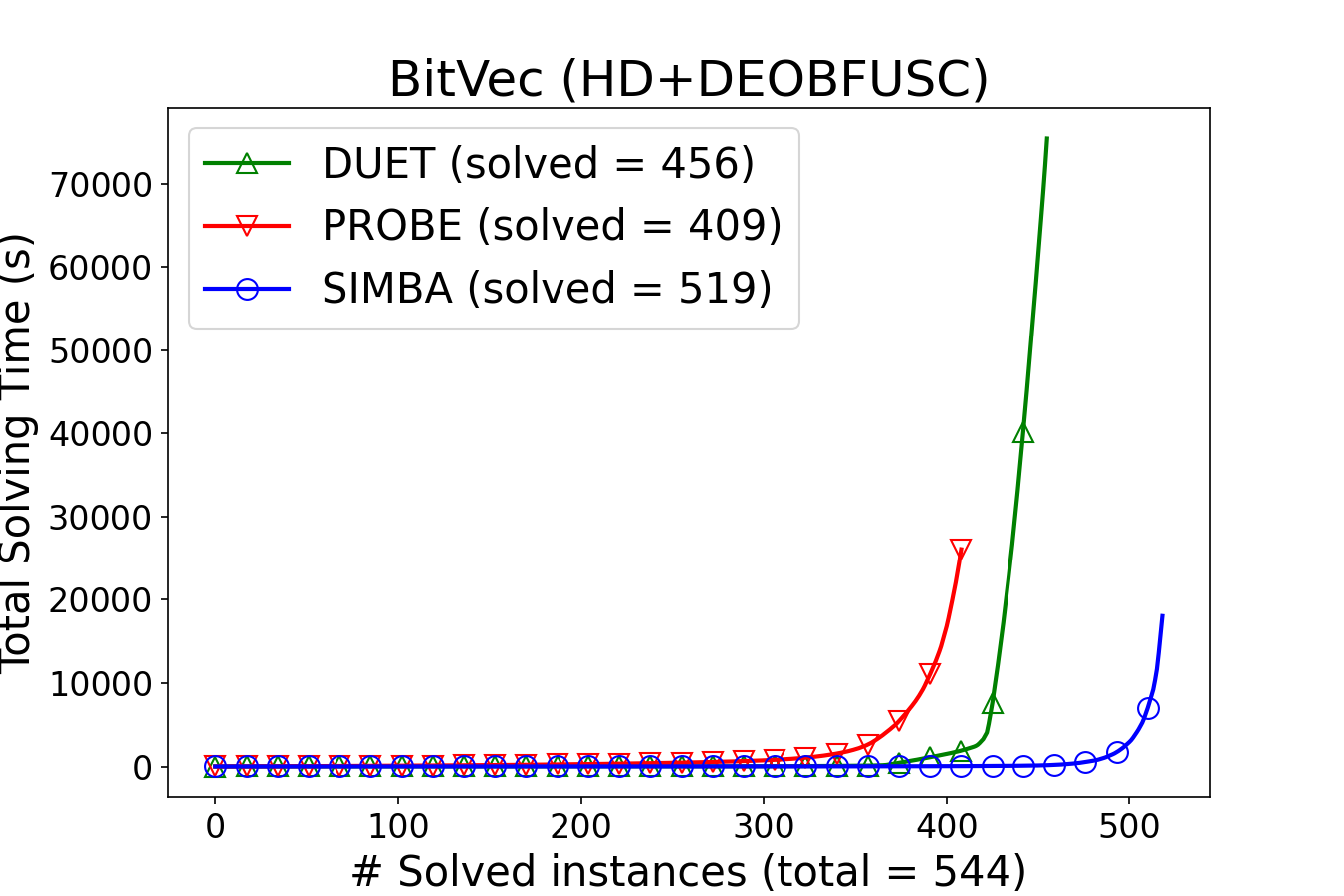
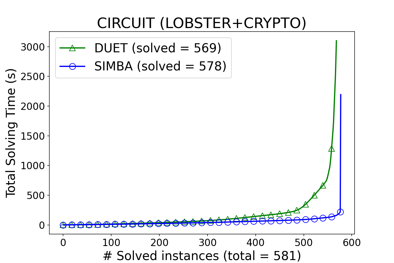
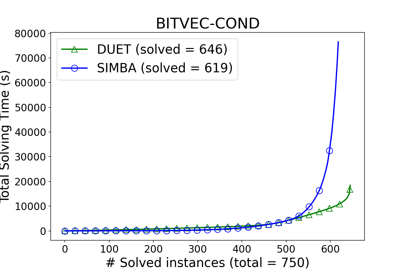
Figure 2. Comparison between Simba and the other baseline solvers on different domains.

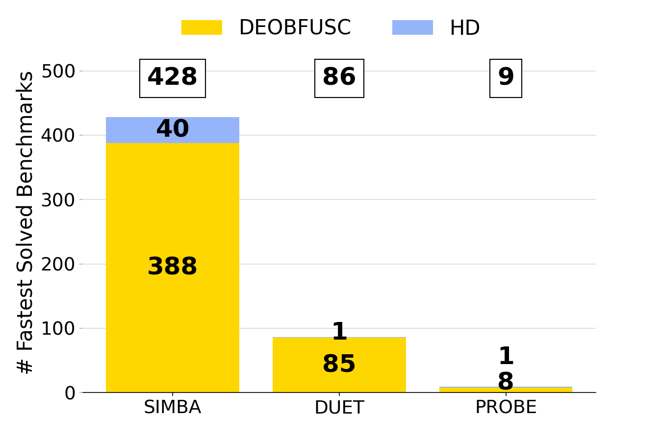
(a) # Fastest solved in the BitVec domain

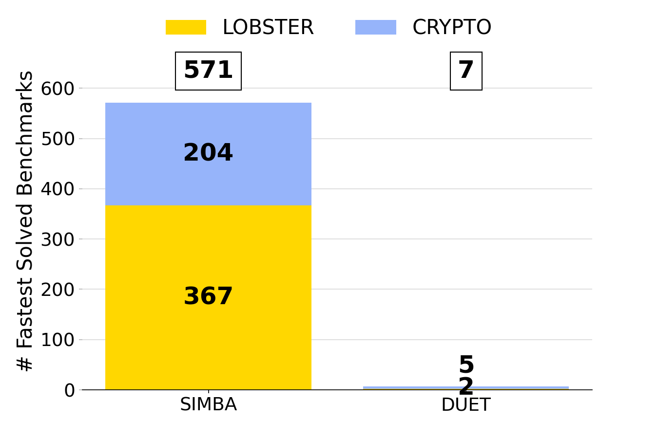
(b) # Fastest solved in the Circuit domain

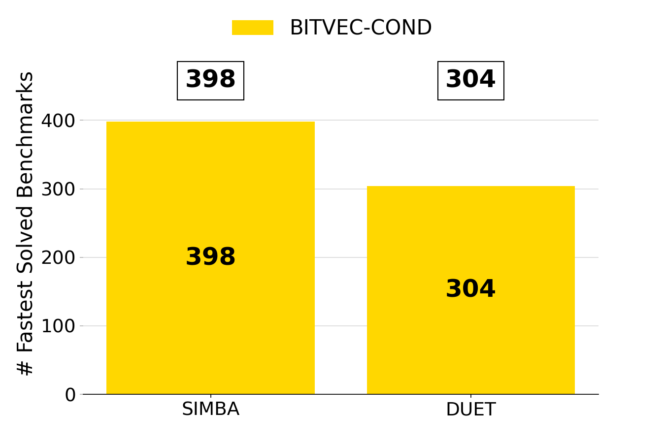
(c) # Fastest solved in the BitVec-Cond domain

Benchmark	# Solved			Time (Average)			Time (Median)			Size (Average)			Size (Median)
category​	Simba	Duet	Probe	S	D	P	S	D	P	S	D	P	S	D	P
HD ​	42	36	31	5.7	42.7	11.8	0.1	0.2	1.0	7.7	8.5	6.5	6	8	5
Deobfusc ​	477	420	378	37.3	175.8	68.0	0.0	0.1	2.9	9.6	10.0	7.9	9	9	8
BitVec-Cond ​	619	646	-	123.6	28.6	-	5.3	5.7	-	269.6	350.6	-	137	46	-
Lobster​	369	369	-	0.4	7.4	-	0.2	0.8	-	12.9	10.9	-	13	11	-
Crypto​	209	200	-	9.7	1.8	-	0.1	0.2	-	11.9	12.8	-	11	12	-
Overall ​	1716	1671	409	56.4	58.0	63.7	0.2	1.7	2.7	107.1	145.4	7.8	15	13	8

(d) Statistics for the solving times and solution sizes. All times are in seconds. Probe could not run for the Circuit and BitVec-Cond domain. The number of problems in the HD, Deobfusc, Lobster, Crypto, and BitVec-Cond categories are 44, 500, 369, 212, and 750 respectively (1875 in total).

Figure 3. Main result comparing the performance of Simba, Duet, and Probe (breakdown by categories). The timeout is set to one hour.

We evaluate Simba on all the benchmarks and compare it with Duet and Probe. For each instance, we measure the running time of synthesis and the size of the synthesized program, using a timeout of one hour.

The results are summarized in Fig. 3. Fig. 3(d) shows the statistics of the solving times and solution sizes, and Fig. 3(a) and 3(b) show the number of instances solved with the fastest time for each domain per solver. Because Probe is not applicable to the Circuit and BitVec-Cond domains, the results for Probe on these domains are not shown.

Overall, Simba outperforms the other baseline tools both in terms of the number of instances solved and the average solving time. As shown in Fig. 3(d), Simba solves 1716 instances, while Duet and Probe solve 1671 and 409 instances respectively. Simba is the fastest solver in 1397 instances (75% of the total), while Duet is the fastest in 397 instances. Fig. 2 shows the cactus plot of the solving times for Simba, Duet, and Probe. The horizontal axis represents the number of solved instances and the vertical axis represents the cumulative solving time. The plot suggests that Simba solves more instances than Duet and Probe in a shorter time.

In comparison to Duet, Simba is more efficient in the BitVec domain and Circuit domain, while Duet is more efficient in the BitVec-Cond domain. Since Simba performs the forward-backward analysis for each input-output example, the number of examples affects the efficiency. In the BitVec-Cond domain, the number of examples is unusually large (up to 1000), which makes Simba inefficient. On the other hand, Duet is able to handle the large number of examples efficiently. However, for the other domains (particularly BitVec), Simba outperforms Duet because Duet’s inverse semantics often creates sub-problems that are hard to solve whereas Simba does not generate such sub-problems.

We measure solution quality by solution sizes in AST nodes. According to Occam’s razor, smaller solutions are better since they are less likely to overfit the input-output examples. In general, Probe generates the smallest solutions (with average sizes of 6.5 and 7.9 for two domains), although Simba is also capable of generating solutions of similar sizes (with average sizes of 7.7 and 9.6). The slight gap between the two tools can be attributed to the fact that Simba can solve instances that Probe cannot solve due to its limited scalability. For example, Simba’s solutions for the two domains not solved by Probe have average sizes of 10.5 and 13.1, respectively, while Simba’s solutions to the ones solved by both tools have average sizes of 6.8 and 8.6, respectively.

5.2.0.1 Result in Detail.

Table 1. Results for 25 randomly chosen benchmark problems (5 for each category), where Time gives synthesis time, $T_{A}$ gives time spent for forward and backward analysis, and $|P|$ shows the size of the synthesized program (measured by number of AST nodes).

Benchmark	Benchmark	Probe		Duet		Simba
category​		Time	$|P|$	Time	$|P|$	Time	$T_{A}$	$|P|$
HD	hd-03-d5-prog	0.85	4	1.19	4	0.06	0.00	4
	hd-07-d0-prog	0.92	6	0.09	6	0.07	0.00	6
	hd-14-d5-prog	4.91	9	¿1h	-	0.60	0.26	9
	hd-19-d1-prog	¿1h	-	¿1h	-	10.79	7.07	19
	hd-20-d1-prog	¿1h	-	228.98	15	98.22	0.22	15
Deobfusc	target_9	¿1h	-	2310.23	16	31.45	2.85	16
	target_119	0.87	5	0.02	8	0.05	0.03	9
	target_385	15.35	9	37.46	10	0.33	0.25	9
	target_410	¿1h	-	2635.78	16	69.38	3.06	16
	target_449	2.61	7	0.01	7	0.03	0.00	7
BitVec-Cond	133_1000	-	-	48.18	35	166.55	6.89	139
	23_10	-	-	340.75	62	0.89	0.40	15
	60_100	-	-	6.90	14	0.15	0.10	14
	icfp_gen_10.7	-	-	4.68	67	1.19	0.20	192
	icfp_gen_14.1	-	-	6.29	154	49.61	37.75	415
Lobster	hd09.eqn_45_0	-	-	21.95	15	11.09	0.32	13
	longest_1bit-opt.eqn_63_1	-	-	0.59	13	0.17	0.01	11
	longest_1bit-opt.eqn_75_1	-	-	1.31	14	0.24	0.01	15
	p03.eqn_38_2	-	-	0.22	9	0.11	0.01	9
	p09.eqn_49_1	-	-	0.24	7	0.19	0.01	9
Crypto	CrCy_2-P6_2-P6	-	-	193.68	20	0.65	0.07	20
	CrCy_5-P9-D5-sIn	-	-	0.13	11	0.11	0.00	11
	CrCy_8-P12-D5-sIn4	-	-	0.21	11	0.14	0.01	11
	CrCy_8-P12-D7-sIn5	-	-	1.99	19	0.63	0.04	19
	CrCy_10-sbox2-D5-sIn11	-	-	0.28	9	0.13	0.00	9

We study the results for each domain in detail. Table 1 shows the detailed results on randomly chosen 25 problems (5 for each category). The results suggest the significant impact of the forward and backward analyses. For example, for hd-20-d1-prog, Simba discarded $11,365$ out of total $11,710$ partial programs generated during the synthesis (97.1%) with a small overhead of $0.22$ seconds. For target-410, $187,858$ out of $188,501$ partial programs (99.7%) are early pruned by Simba with an acceptable overhead of $3.06$ seconds. Furthermore, we observe that even partial programs are not discarded, the holes in the partial programs are highly constrained by the necessary preconditions, thereby significantly reducing the number of components to be explored for the completion of the partial programs. On the other hand, Duet and Probe do not perform such pruning and thus generate many unlikely candidates, taking 10 to 1000 times longer than Simba.

5.2.0.2 Analysis of the Impact of the Number of Examples.

We study the impact of the number of examples on the performance of Simba. Since the forward-backward analysis is performed as many times as the number of examples, the number of examples affects the efficiency, but the impact on efficiency is not significant in practice as long as the number of examples is not too large. We have conducted experiments with 500 deobfuscation benchmarks with the number of examples ranging from 5 to 20. When the number of examples given to Simba are 5, 10, and 20, the average synthesis time is 29.8, 31.0, and 37.3 seconds, respectively. In all cases, the average solution size is 9.5. In other words, the average synthesis time increased by just 25% when the number of examples increased fourfold (from 5 to 20).

5.2.0.3 Summary of Results.

Simba solves harder synthesis problems more quickly compared to the state-of-the-art baseline tools in diverse domains.

5.3. Efficacy of Our Abstract Interpretation-based Pruning

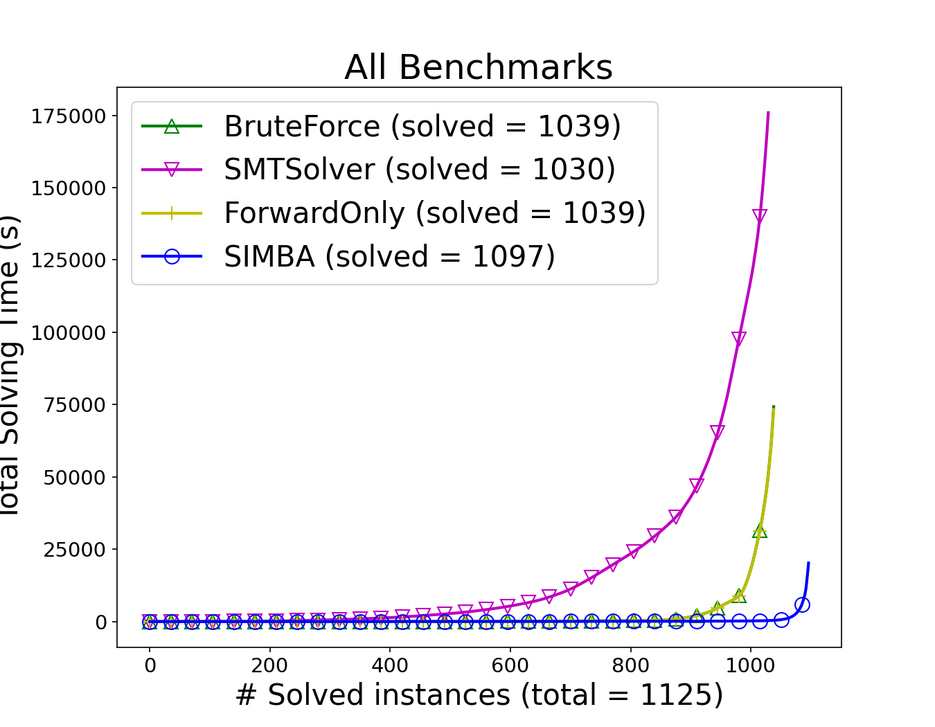
(a) Performance of different variants of Simba

Benchmark	# Solved				Time (Average)
category​	S	FW	SMT	BF	S	FW	SMT	BF
HD ​	42	41	40	41	5.7	12.9	163.6	13.4
Deobfusc​	477	421	424	421	37.3	128.8	178.7	131.2
Lobster​	369	368	358	368	0.4	43.7	234.9	43.5
Crypto​	209	209	208	209	9.7	11.8	45.7	11.9
Overall​	1097	1039	1030	1039	18.4	70.5	170.8	71.5

(b) Statistics for the solving times. S, FW, SMT, and BF denote Simba, ForwardOnly, SMTSolver, and BruteForce variants respectively.

Figure 4. Result for the ablation study.

We now evaluate the effectiveness of our abstract interpretation-based pruning. For this purpose, we compare the performance of three variants of Simba, each using a different combination:

• Simba with the forward and backward analyses (i.e., the original Simba)

• ForwardOnly only with the forward analysis

• BruteForce without any pruning technique (i.e., only with the bidirectional search strategy)

• SMTSolver equipped with the SMT-based pruning. It checks the feasibility of each partial program by checking the satisfiability of an SMT formula. The formula encodes the partial program under construction and the desired input-output behavior of the program. A similar approach was used in Morpheus (Feng et al., 2017) to prune the search space. Because the SMT solving is without any approximation, it is expected to be more accurate than the abstract interpretation-based pruning at the cost of higher computational cost.

By comparing the performance of these variants, we aim to understand

• the overall impact of our abstract interpretation-based pruning (Simba vs. BruteForce)

• the necessity of the backward analysis (Simba vs. ForwardOnly vs. BruteForce)

• the cost-effectiveness of using an abstract interpreter (ForwardOnly vs. SMTSolver)

Fig. 4 shows the results of the ablation study (Fig. 4(b) shows the statistics for the solving times and Fig. 4(a) shows the cactus plots). We exclude the BitVec-Cond benchmarks which require extensive case-splitting dealt with by the divide-and-conquer strategy (Alur et al., 2017) to focus on evaluating the core idea of our approach.

The first observation is that our abstract interpretation-based pruning is effective in reducing the search space (1097 solved by Simba vs. 1039 solved by BruteForce). The second observation is that the backward analysis is necessary to prune the search space effectively because BruteForce and ForwardOnly are almost the same whereas Simba is much better than ForwardOnly. The third observation is that using the SMT solver is more expensive than using an abstract interpreter (1039 solved by ForwardOnly vs. 1030 solved by SMTSolver). Though the SMT solver is more accurate than the abstract interpreter, the success rate of pruning by the SMT solver is not enough to offset the increased computational cost. Thus, using the abstract interpreter strikes a good balance between the precision and the computational cost. As an example, for the benchmark hd-14-d1, by the SMTSolver variant, the SMT solver is invoked 2,247 times and used to prune 1,091 partial programs. This takes 49.08 seconds out of 52.33 seconds spent for solving the benchmark. On the other hand, by Simba, the forward-backward analysis is invoked 1,230 times to prune 1,127 partial programs. This takes only 0.06 second out of 0.15 second spent for solving the benchmark. This shows the cost-effectiveness of using the abstract interpreter.

5.3.0.1 Summary of Results.

Both of the forward and backward analyses are necessary to prune the search space effectively. In addition, using the SMT solver is more expensive than using an abstract interpreter.

6. Related Work

6.0.0.1 Synthesis with Abstract Interpretation.

Most of the previous pruning approaches to program synthesis by abstract interpretation have employed forward abstract interpretation only (So and Oh, 2017; Wang et al., 2017a; Feng et al., 2017; Singh and Solar-Lezama, 2011; Vechev et al., 2010; Wang et al., 2017b). Contrary to these approaches, our technique uses both forward and backward reasoning to derive necessary preconditions for missing expressions and use them to effectively prune the search space.

Pailoor et al. (2021) accelerate synthesis via backward reasoning to check if necessary preconditions can be met by each candidate program. In their setting, a necessary precondition for a partial program $P$ is a constraint on $P$’s inputs that must be satisfied by any completion of $P$ in order for $P$ to satisfy a given contraint over a desired new data structure. If the condition is falsified by any input, the partial program is discarded. Such a necessary precondition can be computed by the standard weakest precondition method. However, there is no synergistic combination of forward and backward reasoning, thereby potentially limiting the pruning power.

To the best of our knowledge, Mukherjee et al. (2020) is the only prior work that uses both forward and backward abstract interpretation to prune the search space of synthesis. However, a synergistic combination of forward and backward analyses is missing. In this work, the forward and backward analyses are performed separately without any interaction between them. In addition, their work is limited to LLVM superoptimization, whereas our work is applicable to a wide range of inductive synthesis problems by targetting the SyGuS specification language.

In contrast to our work that uses fixed abstract domains throughout the synthesis process, another line of work is based on abstraction refinement (Wang et al., 2017b, 2018; Vechev et al., 2010; Guo et al., 2019). In these approaches, programs that do not satisfy the specification are used to iteratively refine the domain until a solution is found. Blaze (Wang et al., 2017b) with its extension (Wang et al., 2018) automatically learns predicate abstract domains from a given set of predicate templates and training synthesis problems. This approach is useful when there is no expert having a good understanding of the target application domain. Our work shows that highly precise abstractions for abstract interpretation can significantly improve the synthesis performance without abstraction refinement. We expect our key idea of using forward and backward analyses can be applied to abstraction refinement-based approaches to further improve the synthesis performance.

6.0.0.2 Iterated Forward/Backward Analysis.

The combination of forward and backward static analyses, which was first introduced in (Cousot, 1978), has been studied in the context of program verification (Cousot and Cousot, 1992; Massé, 2001; Dimovski and Legay, 2020; Kanagasabapathi and Thushara, 2020; Kafle and Gallagher, 2015), model checking (Cousot and Cousot, 1999), counterexample generation for failed specifications (Yin et al., 2019; Yin, 2019), and filtering spurious static analysis alarms (Rival, 2005). In general, iterated forward and backward analyses increase the precision of the analysis at the cost of increased analysis time.

To the best of our knowledge, our work is the first to use the iterated forward and backward analyses for inductive synthesis. Our key finding is that a highly precise analysis employing both forward and backward reasoning can increase the success rate of pruning, which is enough to offset the increased analysis time.

6.0.0.3 Abstract Domains for Bit-Vector Arithmetic.

There is a large body of work on abstract domains for bit-vector arithmetic. In the following, we briefly describe a few of them. Miné (2012) and Regehr and Duongsaa (2006) proposed to use a combination of the interval domain and the bitwise domain. Some of our forward abstract transfer functions are borrowed from these works. The wrapped interval domain (Gange et al., 2015) can precisely track effects of overflow and underflow by wrapping the bit-vector values around the minimum and maximum bit-vector values. Sharma and Reps (2017) proposed a framework for transforming numeric abstract domains over integers to bit-vector domains. Simon and King (2007) proposed a wrap-around operator for polyhedra to track the wrap-around effects.

To the best of our knowledge, none of the existing domains for bit-vectors provide backward abstract transfer functions. As already shown in our experiments, the backward abstract interpretation is crucial for pruning the search space. Therefore, to employ the existing domains for our approach, one needs to develop backward abstract transfer functions for them.

6.0.0.4 Domain Specializations for Inductive Synthesis.

Recent works have demonstrated significant performance gains by exploiting domain knowledge in various forms such as domain-specific languages (Gulwani, 2011; Rolim et al., 2017; Kini and Gulwani, 2015), probabilistic models (Barke et al., 2020; Lee et al., 2018), inverse semantics (Lee, 2021), and templates (Inala et al., 2016). In particular, Duet (Lee, 2021) combines the bidirectional search with specialized inverse semantics (also called witness functions) that return the set of possible inputs that can produce a given output. Our work combines the birectional search with abstract interpretation. Our experiments show that highly precise abstract semantics can provide significant performance gains that are complementary to those achieved by other domain specializations such as inverse semantics and probabilistic models, and it is promising to incorporate our approach into the previous approaches.

7. Future Work

A possible extension of our approach is to support other theories in SyGuS such as integer arithmetic and string theory. Due to insufficient precision of a single abstract domain, multiple abstract domains are necessary including forward/backward abstract transfer functions and a reduction operator to define a reduced product of those abstract domains. For integer arithmetic, a reduced product of existing non-relational abstract domains such as the interval domain (Cousot and Cousot, 1977) and the congruence domain (Granger, 1989) can be used. Furthermore, relational domains (Miné, 2006; Singh et al., 2017) can aid in tracking the relations between different program holes and input variables. For strings, abstract domains using prefixes, suffixes, and simple regular expressions (Costantini et al., 2011), pushdown automata (Kim and Choe, 2011), and parse stacks (Doh et al., 2009) can be used. Another possible extension is to synthesize programs with loops. In contrast to our current loop-free setting, the forward and backward analyses may require advanced widening/narrowing operators (e.g., widening with inferred thresholds (Lakhdar-Chaouch et al., 2011)) to expedite the convergence of the fixpoint iteration while maintaining precision.

8. Conclusion

We presented a novel program synthesis algorithm that effectively prunes the search space by using a forward and backward abstract interpretation. Our implementation Simba and its evaluation showed that the performance is significantly better than the existing state-of-the-art synthesis systems Duet and Probe. The key to enable this performance and scalability of inductive program synthesis is to combine a forward abstract interpretation with a backward one to rapidly narrow down the search space. Our experiments also showed that using SMT solver on behalf of such sophisticated static analysis does not scale.

8.0.0.1 Data-Availability Statement.

The artifact is available at Zenodo(Yoon et al., 2023).

References

- (1)
- Alur et al. (2013) Rajeev Alur, Rastislav Bodik, Garvit Juniwal, Milo M. K. Martin, Mukund Raghothaman, Sanjit A. Seshia, Rishabh Singh, Armando Solar-Lezama, Emina Torlak, and Abhishek Udupa. 2013. Syntax-guided synthesis. In Formal Methods in Computer-Aided Design (FMCAD ’13).
- Alur et al. (2017) Rajeev Alur, Arjun Radhakrishna, and Abhishek Udupa. 2017. Scaling Enumerative Program Synthesis via Divide and Conquer. In Tools and Algorithms for the Construction and Analysis of Systems, Axel Legay and Tiziana Margaria (Eds.). Springer Berlin Heidelberg, Berlin, Heidelberg, 319–336.
- Barke et al. (2020) Shraddha Barke, Hila Peleg, and Nadia Polikarpova. 2020. Just-in-Time Learning for Bottom-up Enumerative Synthesis. Proc. ACM Program. Lang. 4, OOPSLA, Article 227 (nov 2020), 29 pages. https://doi.org/10.1145/3428295
- Barrett et al. (2010) Clark W. Barrett, Aaron Stump, and Cesare Tinelli. 2010. The SMT-LIB Standard Version 2.0.
- Blazytko et al. (2017) Tim Blazytko, Moritz Contag, Cornelius Aschermann, and Thorsten Holz. 2017. Syntia: Synthesizing the Semantics of Obfuscated Code. In 26th USENIX Security Symposium (USENIX Security 17). USENIX Association, Vancouver, BC, 643–659. https://www.usenix.org/conference/usenixsecurity17/technical-sessions/presentation/blazytko
- Costantini et al. (2011) Giulia Costantini, Pietro Ferrara, and Agostino Cortesi. 2011. Static Analysis of String Values. In Formal Methods and Software Engineering, Shengchao Qin and Zongyan Qiu (Eds.). Springer Berlin Heidelberg, Berlin, Heidelberg, 505–521.
- Cousot (1978) Patrick Cousot. 1978. Méthodes itératives de construction et d’approximation de points fixes d’opérateurs monotones sur un treillis, analyse sémantique des programmes. Habilitation à diriger des recherches. Institut National Polytechnique de Grenoble - INPG ; Université Joseph-Fourier - Grenoble I. https://tel.archives-ouvertes.fr/tel-00288657 Universités : Université scientifique et médicale de Grenoble et Institut national polytechnique de Grenoble.
- Cousot (2021) Patrick Cousot. 2021. Principles of Abstract Interpretation. The MIT Press.
- Cousot and Cousot (1977) Patrick Cousot and Radhia Cousot. 1977. Abstract Interpretation: A Unified Lattice Model for Static Analysis of Programs by Construction or Approximation of Fixpoints. In Proceedings of The ACM SIGPLAN-SIGACT Symposium on Principles of Programming Languages. 238–252.
- Cousot and Cousot (1992) Patrick Cousot and Rahida Cousot. 1992. Abstract Interpretation and Application to Logic Programs. J. Log. Program. 13, 2–3 (jul 1992), 103–179. https://doi.org/10.1016/0743-1066(92)90030-7
- Cousot and Cousot (1999) Patrick Cousot and Radhia Cousot. 1999. Refining Model Checking by Abstract Interpretation. Automated Software Engineering 6, 1 (1999), 69–95. https://doi.org/10.1023/A:1008649901864
- David et al. (2020) Robin David, Luigi Coniglio, and Mariano Ceccato. 2020. QSynth - A Program Synthesis based approach for Binary Code Deobfuscation. Proceedings 2020 Workshop on Binary Analysis Research (2020).
- De Moura and Bjorner (2008) Leonardo De Moura and Nikolaj Bjorner. 2008. Z3: An Efficient SMT Solver. In Proceedings of the Theory and Practice of Software, 14th International Conference on Tools and Algorithms for the Construction and Analysis of Systems (Budapest, Hungary) (TACAS’08). Springer-Verlag, Berlin, Heidelberg, 337–340.
- Dimovski and Legay (2020) Aleksandar S. Dimovski and Axel Legay. 2020. Computing Program Reliability Using Forward-Backward Precondition Analysis and Model Counting. In Fundamental Approaches to Software Engineering, Heike Wehrheim and Jordi Cabot (Eds.). Springer International Publishing, Cham, 182–202.
- Doh et al. (2009) Kyung-Goo Doh, Hyunha Kim, and David A. Schmidt. 2009. Abstract Parsing: Static Analysis of Dynamically Generated String Output Using LR-Parsing Technology. In Proceedings of the 16th International Symposium on Static Analysis (Los Angeles, CA) (SAS ’09). Springer-Verlag, Berlin, Heidelberg, 256–272. https://doi.org/10.1007/978-3-642-03237-0_18
- Feng et al. (2017) Yu Feng, Ruben Martins, Jacob Van Geffen, Isil Dillig, and Swarat Chaudhuri. 2017. Component-Based Synthesis of Table Consolidation and Transformation Tasks from Examples. SIGPLAN Not. 52, 6 (jun 2017), 422–436. https://doi.org/10.1145/3140587.3062351
- Gange et al. (2015) Graeme Gange, Jorge A. Navas, Peter Schachte, Harald Sondergaard, and Peter J. Stuckey. 2015. Interval Analysis and Machine Arithmetic: Why Signedness Ignorance Is Bliss. ACM Trans. Program. Lang. Syst. 37, 1, Article 1 (jan 2015), 35 pages. https://doi.org/10.1145/2651360
- Granger (1989) Philippe Granger. 1989. Static analysis of arithmetical congruences. International Journal of Computer Mathematics 30, 3-4 (1989), 165–190. https://doi.org/10.1080/00207168908803778 arXiv:https://doi.org/10.1080/00207168908803778
- Granger (1992) Philippe Granger. 1992. Improving the results of static analyses of programs by local decreasing iterations. In Foundations of Software Technology and Theoretical Computer Science, Rudrapatna Shyamasundar (Ed.). Springer Berlin Heidelberg, Berlin, Heidelberg, 68–79.
- Gulwani (2011) Sumit Gulwani. 2011. Automating String Processing in Spreadsheets Using Input-output Examples. In Proceedings of the 38th Annual ACM SIGPLAN-SIGACT Symposium on Principles of Programming Languages (Austin, Texas, USA) (POPL ’11).
- Guo et al. (2019) Zheng Guo, Michael James, David Justo, Jiaxiao Zhou, Ziteng Wang, Ranjit Jhala, and Nadia Polikarpova. 2019. Program Synthesis by Type-Guided Abstraction Refinement. Proc. ACM Program. Lang. 4, POPL, Article 12 (dec 2019), 28 pages. https://doi.org/10.1145/3371080
- Hu et al. (2020) Qinheping Hu, John Cyphert, Loris D’Antoni, and Thomas Reps. 2020. Exact and Approximate Methods for Proving Unrealizability of Syntax-Guided Synthesis Problems. In Proceedings of the 41st ACM SIGPLAN Conference on Programming Language Design and Implementation (London, UK) (PLDI 2020). Association for Computing Machinery, New York, NY, USA, 1128–1142. https://doi.org/10.1145/3385412.3385979
- Inala et al. (2016) Jeevana Priya Inala, Rohit Singh, and Armando Solar-Lezama. 2016. Synthesis of Domain Specific CNF Encoders for Bit-Vector Solvers. In Theory and Applications of Satisfiability Testing – SAT 2016, Nadia Creignou and Daniel Le Berre (Eds.). Springer International Publishing, Cham, 302–320.
- Kafle and Gallagher (2015) Bishoksan Kafle and John P. Gallagher. 2015. Constraint Specialisation in Horn Clause Verification. In Proceedings of the 2015 Workshop on Partial Evaluation and Program Manipulation (Mumbai, India) (PEPM ’15). Association for Computing Machinery, New York, NY, USA, 85–90. https://doi.org/10.1145/2678015.2682544
- Kanagasabapathi and Thushara (2020) Somasundaram Kanagasabapathi and M. G. Thushara. 2020. Forward and Backward Static Analysis for Critical numerical accuracy in Floating Point Programs. Comput. Sci. 21 (2020).
- Kim and Choe (2011) Se-Won Kim and Kwang-Moo Choe. 2011. String Analysis as an Abstract Interpretation. In Verification, Model Checking, and Abstract Interpretation, Ranjit Jhala and David Schmidt (Eds.). Springer Berlin Heidelberg, Berlin, Heidelberg, 294–308.
- Kini and Gulwani (2015) Dileep Kini and Sumit Gulwani. 2015. FlashNormalize: Programming by Examples for Text Normalization. In Proceedings of the 24th International Conference on Artificial Intelligence (Buenos Aires, Argentina) (IJCAI’15). AAAI Press, 776–783.
- Lakhdar-Chaouch et al. (2011) Lies Lakhdar-Chaouch, Bertrand Jeannet, and Alain Girault. 2011. Widening with Thresholds for Programs with Complex Control Graphs. In Automated Technology for Verification and Analysis, Tevfik Bultan and Pao-Ann Hsiung (Eds.). Springer Berlin Heidelberg, Berlin, Heidelberg, 492–502.
- Lee et al. (2020) DongKwon Lee, Woosuk Lee, Hakjoo Oh, and Kwangkeun Yi. 2020. Optimizing Homomorphic Evaluation Circuits by Program Synthesis and Term Rewriting. In Proceedings of the 41st ACM SIGPLAN Conference on Programming Language Design and Implementation (London, UK) (PLDI 2020). Association for Computing Machinery, New York, NY, USA, 503–518. https://doi.org/10.1145/3385412.3385996
- Lee (2021) Woosuk Lee. 2021. Combining the top-down propagation and bottom-up enumeration for inductive program synthesis. Proceedings of the ACM on Programming Languages 5, POPL (2021), 1–28.
- Lee et al. (2018) Woosuk Lee, Kihong Heo, Rajeev Alur, and Mayur Naik. 2018. Accelerating Search-Based Program Synthesis Using Learned Probabilistic Models. In Proceedings of the 39th ACM SIGPLAN Conference on Programming Language Design and Implementation (Philadelphia, PA, USA) (PLDI 2018). Association for Computing Machinery, New York, NY, USA, 436–449. https://doi.org/10.1145/3192366.3192410
- Massé (2001) Damien Massé. 2001. Combining Forward And Backward Analyses of Temporal Properties. In Programs as Data Objects, Olivier Danvy and Andrzej Filinski (Eds.). Springer Berlin Heidelberg, Berlin, Heidelberg, 103–116.
- Menguy et al. (2021) Grégoire Menguy, Sébastien Bardin, Richard Bonichon, and Cauim de Souza Lima. 2021. Search-Based Local Black-Box Deobfuscation: Understand, Improve and Mitigate. In Proceedings of the 2021 ACM SIGSAC Conference on Computer and Communications Security (Virtual Event, Republic of Korea) (CCS ’21). Association for Computing Machinery, New York, NY, USA, 2513–2525. https://doi.org/10.1145/3460120.3485250
- Miné (2006) Antoine Miné. 2006. The octagon abstract domain. Higher-Order and Symbolic Computation 19, 1 (2006), 31–100. https://doi.org/10.1007/s10990-006-8609-1
- Miné (2012) Antoine Miné. 2012. Abstract domains for bit-level machine integer and floating-point operations. In WING’12 - 4th International Workshop on invariant Generation. Manchester, United Kingdom, 16. https://hal.archives-ouvertes.fr/hal-00748094
- Mukherjee et al. (2020) Manasij Mukherjee, Pranav Kant, Zhengyang Liu, and John Regehr. 2020. Dataflow-Based Pruning for Speeding up Superoptimization. Proc. ACM Program. Lang. 4, OOPSLA, Article 177 (nov 2020), 24 pages. https://doi.org/10.1145/3428245
- Pailoor et al. (2021) Shankara Pailoor, Yuepeng Wang, Xinyu Wang, and Isil Dillig. 2021. Synthesizing Data Structure Refinements from Integrity Constraints. In Proceedings of the 42nd ACM SIGPLAN International Conference on Programming Language Design and Implementation (Virtual, Canada) (PLDI 2021). Association for Computing Machinery, New York, NY, USA, 574–587. https://doi.org/10.1145/3453483.3454063
- Past SyGuS Competition (2020) Past SyGuS Competition. 2020. https://sygus.org/comp/.
- Polikarpova et al. (2016) Nadia Polikarpova, Ivan Kuraj, and Armando Solar-Lezama. 2016. Program Synthesis from Polymorphic Refinement Types. In Proceedings of the 37th ACM SIGPLAN Conference on Programming Language Design and Implementation (Santa Barbara, CA, USA) (PLDI ’16). Association for Computing Machinery, New York, NY, USA, 522–538. https://doi.org/10.1145/2908080.2908093
- Regehr and Duongsaa (2006) John Regehr and Usit Duongsaa. 2006. Deriving Abstract Transfer Functions for Analyzing Embedded Software. In Proceedings of the 2006 ACM SIGPLAN/SIGBED Conference on Language, Compilers, and Tool Support for Embedded Systems (Ottawa, Ontario, Canada) (LCTES ’06). Association for Computing Machinery, New York, NY, USA, 34–43. https://doi.org/10.1145/1134650.1134657
- Rival (2005) Xavier Rival. 2005. Understanding the Origin of Alarms in Astrée. In Static Analysis, Chris Hankin and Igor Siveroni (Eds.). Springer Berlin Heidelberg, Berlin, Heidelberg, 303–319.
- Rival and Yi (2020) Xavier Rival and Kwangkeun Yi. 2020. Introduction to Static Analysis: an Abstract Interpretation Perspective. The MIT Press.
- Rolim et al. (2017) Reudismam Rolim, Gustavo Soares, Loris D’Antoni, Oleksandr Polozov, Sumit Gulwani, Rohit Gheyi, Ryo Suzuki, and Björn Hartmann. 2017. Learning Syntactic Program Transformations from Examples. In Proceedings of the 39th International Conference on Software Engineering (Buenos Aires, Argentina) (ICSE’17). IEEE Press, 404–415. https://doi.org/10.1109/ICSE.2017.44
- Sharma and Reps (2017) Tushar Sharma and Thomas Reps. 2017. Sound Bit-Precise Numerical Domains. In Verification, Model Checking, and Abstract Interpretation, Ahmed Bouajjani and David Monniaux (Eds.). Springer International Publishing, Cham, 500–520.
- Simon and King (2007) Axel Simon and Andy King. 2007. Taming the Wrapping of Integer Arithmetic. In Static Analysis, Hanne Riis Nielson and Gilberto Filé (Eds.). Springer Berlin Heidelberg, Berlin, Heidelberg, 121–136.
- Singh et al. (2017) Gagandeep Singh, Markus Püschel, and Martin Vechev. 2017. Fast Polyhedra Abstract Domain. In Proceedings of the 44th ACM SIGPLAN Symposium on Principles of Programming Languages (Paris, France) (POPL ’17). Association for Computing Machinery, New York, NY, USA, 46–59. https://doi.org/10.1145/3009837.3009885
- Singh and Solar-Lezama (2011) Rishabh Singh and Armando Solar-Lezama. 2011. Synthesizing Data Structure Manipulations from Storyboards. In Proceedings of the 19th ACM SIGSOFT Symposium and the 13th European Conference on Foundations of Software Engineering (Szeged, Hungary) (ESEC/FSE ’11). Association for Computing Machinery, New York, NY, USA, 289–299. https://doi.org/10.1145/2025113.2025153
- So and Oh (2017) Sunbeom So and Hakjoo Oh. 2017. Synthesizing Imperative Programs from Examples Guided by Static Analysis. In Static Analysis, Francesco Ranzato (Ed.). Springer International Publishing, Cham, 364–381.
- Solar-Lezama et al. (2006) Armando Solar-Lezama, Liviu Tancau, Rastislav Bodik, Sanjit Seshia, and Vijay Saraswat. 2006. Combinatorial Sketching for Finite Programs. In Proceedings of the 12th International Conference on Architectural Support for Programming Languages and Operating Systems (San Jose, California, USA) (ASPLOS XII).
- Vechev et al. (2010) Ma[rtin Vechev, Eran Yahav, and Greta Yorsh. 2010. Abstraction-Guided Synthesis of Synchronization. In Proceedings of the 37th Annual ACM SIGPLAN-SIGACT Symposium on Principles of Programming Languages (Madrid, Spain) (POPL ’10). Association for Computing Machinery, New York, NY, USA, 327–338. https://doi.org/10.1145/1706299.1706338
- Wang et al. (2017a) Chenglong Wang, Alvin Cheung, and Rastislav Bodik. 2017a. Synthesizing Highly Expressive SQL Queries from Input-Output Examples. In Proceedings of the 38th ACM SIGPLAN Conference on Programming Language Design and Implementation (Barcelona, Spain) (PLDI 2017). Association for Computing Machinery, New York, NY, USA, 452–466. https://doi.org/10.1145/3062341.3062365
- Wang et al. (2018) Xinyu Wang, Greg Anderson, Isil Dillig, and K. L. McMillan. 2018. Learning Abstractions for Program Synthesis. In Computer Aided Verification, Hana Chockler and Georg Weissenbacher (Eds.). Springer International Publishing, Cham, 407–426.
- Wang et al. (2017b) Xinyu Wang, Isil Dillig, and Rishabh Singh. 2017b. Program Synthesis Using Abstraction Refinement. Proc. ACM Program. Lang. 2, POPL, Article 63 (Dec. 2017), 30 pages. https://doi.org/10.1145/3158151
- Warren (2012) Henry S. Warren. 2012. Hacker’s Delight (2nd ed.). Addison-Wesley Professional.
- Yin (2019) Banghu Yin. 2019. Property Oriented Verification via Iterative Abstract Interpretation. In Proceedings of the 41st International Conference on Software Engineering: Companion Proceedings (Montreal, Quebec, Canada) (ICSE ’19). IEEE Press, 162–164. https://doi.org/10.1109/ICSE-Companion.2019.00067
- Yin et al. (2019) Banghu Yin, Liqian Chen, Jiangchao Liu, Ji Wang, and Patrick Cousot. 2019. Verifying Numerical Programs via Iterative Abstract Testing. In Static Analysis: 26th International Symposium, SAS 2019, Porto, Portugal, October 8–11, 2019, Proceedings (Porto, Portugal). Springer-Verlag, Berlin, Heidelberg, 247–267. https://doi.org/10.1007/978-3-030-32304-2_13
- Yoon et al. (2023) Yongho Yoon, Woosuk Lee, and Kwangkeun Yi. 2023. Artifact of Inductive Program Synthesis via Iterative Forward-Backward Abstract Interpretation. https://doi.org/10.5281/zenodo.7816533